

Submitted:
12 November 2026
Posted:
16 November 2026
You are already at the latest version
Abstract
Feature selection, also known as variable selection, is a foundational problem in econometrics, artificial intelligence, and machine learning. However, widely used procedures may be inaccurate, unstable under collinearity, and sensitive to sampling noise and may lack a principled interpretation in terms of how they allocate explanatory power. This paper develops a feature-selection framework that extends a fair-division approach introduced by Hu ([2020, 2025). We represent the explanatory or forecasting performance of feature subsets as payoffs in a coalitional game subject to sampling uncertainty. Candidate features are partitioned into selected and unselected sets according to their fair-division values, defined using a modified Shapley value. Model uncertainty is represented by a beta-binomial distribution over subset size and a uniform distribution over subsets conditional on size. Each feature’s value combines the expected marginal gain from inclusion with the expected opportunity loss associated with exclusion, thereby treating all candidates symmetrically ex ante under a veil-of-ignorance principle. We further propose a sequential selection algorithm that uses a Monte Carlo approximation and a likelihood-ratio screening rule that admits at most one feature per iteration. Across the simulation designs considered, the procedure attains substantially higher exact-identification rates than those of the benchmark methods, including stepwise, unidirectional, GETS-style, and LASSO-based procedures. The paper also examines residual-share-based hyperparameter calibration, computational complexity, selection consistency, and practical implementation considerations.
Keywords:
feature selection
; variable selection
; model uncertainty
; coalitional game
; likelihood-ratio test
; dichotomous valuation
; Shapley value
; fair division
MSC: 68T20; 62F07; 91A12; 62J07
1. Introduction
Feature selection identifies a subset of essential variables from a larger set of candidate predictors for use in statistical and machine-learning models. It is particularly important in macroeconomics, finance, applied microeconometrics, and other high-dimensional fields, where a parsimonious predictor set can reduce estimator variance, overfitting, and computational burden while improving interpretability, stability, and predictive performance [2,3].
Feature-selection methods are commonly classified into three categories: filter methods, which evaluate variables independently of a predictive model using criteria such as correlation, mutual information, or statistical tests; wrapper methods, which assess subsets of variables according to model performance through procedures such as forward selection, backward elimination, and recursive feature elimination; and embedded methods, in which variable selection is performed during model estimation, as in LASSO, elastic net, and tree-based algorithms [2,8].
However, commonly used automated routines, including stepwise variants, greedy swapping, combinatorial subset search, general-to-specific (GETS-style) simplification, and shrinkage methods such as LASSO, can be unstable when predictors are correlated and vulnerable to selection distortions arising from repeatedly using the same sample for model search and evaluation. In the simulation designs examined below, these procedures exhibit relatively low exact-identification rates.
This paper proposes an approach grounded in the valuation of players in a coalitional game, with features as players and model performance as the payoff. The resulting game differs from a conventional deterministic coalitional game in several respects. In linear regression, for example, the payoff function is subject to sampling error, and the candidate features fall into three groups: essential regressors, redundant regressors, and irrelevant candidates. Under the regularity conditions for least-squares estimation, an irrelevant feature should behave as a dummy player in the population game, contributing no incremental payoff to any coalition. Its estimated contribution, however, need not be zero in finite samples and may nevertheless appear statistically significant in small subsets. A redundant feature, whose explanatory or forecasting power is absorbed by the essential regressors, may be statistically significant in subsets where some essential regressors are absent. As in the Shapley-value framework [9], we seek a method that fairly divides the total attributable variation of the dependent variable. Irrelevant features should receive zero value in the population game, whereas redundant features should become dummy players once the essential features have been accounted for.
The proposed valuation builds on the dichotomous-valuation framework developed by Hu ([5], [6], [7]), in which a feature’s value reflects both (i) marginal gain from inclusion and (ii) opportunity loss from exclusion across a distribution of possible modeling scenarios. Marginal gain and marginal loss receive equal weight. Moreover, all candidate features are treated symmetrically with respect to their ex ante probabilities of selection before observing outcomes. This ex ante uncertainty is represented by a parameterized distribution over candidate subsets. Therefore, unlike filter methods, the valuation approach accounts for relationships among the candidate features.
A boundary condition determines the total contribution to be distributed among the candidate features. Unlike conventional wrapper methods, the proposed framework uses a calibrated slack parameter to reserve the share attributable to the intercept and residual rather than allocating the entire observed payoff to candidate features. The remaining explanatory or predictive power is allocated among the selected features, thereby crowding out redundant candidates. Using this probability distribution and boundary condition, we evaluate many modeling scenarios rather than relying on a single fitted specification, as many embedded methods do. Averaging across these scenarios yields a fair-division value that modifies the conventional Shapley-value allocation. A feature is selected when twice its estimated value meets or exceeds the specified likelihood-ratio critical value. Accordingly, we pair the performance criterion with a statistical decision rule.
The proposed feature-selection procedure achieves high exact-identification rates in the simulation designs considered below. These include Monte Carlo studies that vary the numbers of essential, redundant, and irrelevant features. The studies also examine lag selection in time-series settings and feature selection in the presence of omitted variables. In the controlled simulations reported below, the proposed procedure attains exact-identification rates substantially higher than those of the benchmark methods.
This paper draws on three strands of literature. First, it is linked to cooperative-game allocations of contribution, including the Shapley value and its variants [9,10]. Dichotomous valuation formalizes the idea that features contribute by being either present or absent in alternative models, and that the evaluation must integrate over model uncertainty [6]. Second, the paper contributes to the econometric literature on model selection, including general-to-specific (GETS) and automated selection, where debates emphasize data mining, collinearity, and pre-test biases [4]. Our framework differs by explicitly introducing a probability model over subset scenarios and by valuing both inclusion and exclusion. Third, it relates to penalized regression and LASSO-style approaches [11]. Shrinkage methods are often effective but may select one of several highly correlated covariates in a way that is sensitive to the sample and penalty specification. Our sequential fair-division rule aims to attribute explanatory power via simulated marginal contributions and an explicit significance gate.
In summary, this paper makes four contributions to the literature on variable and feature selection.
- 1.
- A fair-division interpretation of feature selection. We define feature importance as a dichotomous expected marginal contribution that combines gain and loss under a noninformative subset mechanism. Both the amount of performance attributable to candidate features and the classification of those candidates are uncertain.
- 2.
- A beta-binomial mechanism for model uncertainty. We place a beta prior on the inclusion probability and induce a beta-binomial distribution on subset size and a uniform distribution over subsets conditional on size. The prior treats candidate features symmetrically by assigning them equal ex ante inclusion probabilities, and therefore selection is based solely on feature performance.
- 3.
- A sequential algorithm with significance screening. At most one feature is admitted per iteration, limiting the propagation of selection errors across iterations; a likelihood-ratio critical value governs stopping. Under the regularity conditions stated in Appendix A, the selected features converge in probability to the latent essential features.
- 4.
- Simulation evidence. In a controlled linear design with correlated regressors and varying numbers of essential, redundant, and irrelevant features, the fair-division procedure achieves a substantially higher exact-identification rate than those of the benchmark alternatives in these experiments. The method also performs favorably in the reported lag-selection and omitted-variable experiments.
The remainder of the paper is organized as follows. Section 2 reviews the feature-selection problem with a focus on linear regression. Section 3 sets up a coalitional game with modeled uncertainty about coalition formation. Section 4 evaluates each feature in the game. Section 5 describes parameter calibration and the feature-selection algorithm. Section 6 presents simulation evidence under various settings. Section 7 discusses post-selection analysis and practical considerations. Finally, Section 8 discusses the method’s stability, limitations, and possible extensions and concludes the paper. Selection consistency results, proofs, and derivations are provided in the appendices.
2. Feature Selection for Linear Regression
We first introduce the notation used throughout the analysis. Let denote the index set of all candidate features . We assume that the candidate features are not perfectly collinear. Let the unknown subset denote the indices of all essential regressors. For any subset , let denote its cardinality. For convenience, lowercase italic letters denote cardinalities; for example, and . We also use an overbar to denote a singleton set; for example, “" represents the singleton set . Additionally, the symbol ∅ denotes the empty set, “∖" set difference, “∪" set union, “⊊" a proper subset, and “" the sample size.
Suppose that the conditional mean of Y is linear in the essential regressors. For , the corresponding linear model is
for coefficients and residuals . Among the candidate models, we assume that is the unique data-generating model for Y within the candidate model class. The data may be cross-sectional, time-series, or panel in structure. For simplicity, we assume that the regularity conditions of ordinary least-squares estimation hold for all candidate linear regressions, including exogeneity and, where required for the likelihood analysis below, homoskedastic and serially uncorrelated errors.
The objective of the proposed feature-selection procedure is to estimate accurately and efficiently under the fairness criterion developed below. We denote the estimated subset by . Selection accuracy is assessed primarily by the discrepancy between and .
In practice, empirical analysts typically consider only a small fraction of all potential models until they obtain a specification that appears satisfactory in the sample. However, this approach need not be reproducible or optimal under a prespecified criterion. It can yield different results even when the candidate regressors are unchanged. Moreover, the resulting model may fit the historical sample well yet perform poorly out of sample.
2.1. Interdependence Across Features
Beyond model uncertainty, estimating is complicated because a feature’s contribution generally varies across model specifications. Because explanatory variables are often strongly dependent, the incremental contribution of to explaining variation in Y depends on the set of covariates already included in the model.
Figure 1 illustrates how the coefficient on X can depend on the accompanying covariate. In the left panel, the observation y has projection onto the X-axis, corresponding to a positive coefficient. The dashed lines, drawn parallel to the X- and -axes, identify the corresponding coordinate projections. We can decompose y into plus a residual orthogonal to the X– plane. In the right panel, X and y remain unchanged, but is replaced by . Consequently, the projection onto the X-axis corresponds to a negative coefficient.
A feature’s estimated contribution can depend strongly on the accompanying covariates, making importance measures based on a single conditioning set unstable. Averaging appropriately weighted marginal contributions across alternative covariate subsets provides a less specification-dependent measure of overall explanatory or predictive contribution.
2.2. Redundant Features
We categorize all features in into three groups: essential features contained in , redundant features, and irrelevant features. An irrelevant feature has no incremental explanatory power in the population but may be correlated with some elements in . In finite samples, however, an irrelevant feature’s estimated coefficient may differ from zero, even though its population coefficient is zero. A redundant feature may be correlated with Y and with elements of , but its explanatory content is absorbed once the regressors in are controlled for. Variables outside the candidate set indexed by , including omitted or latent determinants, may also affect Y. Their effects may be partly reflected in the intercept , the residual , and the coefficients on included essential features.
In regression , defined in Eq. (1), the estimated contribution of is for . The statistical significance of depends on the relationship between T and , . When many elements of are absent from T, may be significant; otherwise, it may not be. A redundant feature , by contrast, has zero incremental contribution in the population when the model is enlarged from to . This zero-incremental-contribution property also holds for any model containing , under the maintained population assumptions.
Because the significance of redundant features depends on which essential features are already included, we adopt a greedy sequential strategy. At each iteration, the procedure selects the remaining feature with the largest statistically significant contribution and stops when no such contribution remains. After reserving a share of the variation in Y for the residual and, where relevant, the intercept, the procedure sequentially allocates the remaining variability to the candidate with the largest marginal contribution. As essential features are selected, redundant features are crowded out because their incremental explanatory contribution is increasingly absorbed by the selected set. The features admitted before stopping constitute the estimated set .
2.3. Fair Division
The convergence of the selected set to relies on a careful design of the marginal contribution of each feature. Four considerations underlie a fair allocation of the variability in Y.
First, the explanatory power of should be distributed among all candidates. The allocation is designed to limit systematic overfitting and underfitting by recognizing that features outside make no incremental population contribution conditional on . Moreover, the amount attributed to the intercept and residual should not be allocated to the variables in . However, and its explanatory capacity are unknown.
Second, given any model , the marginal contribution of an essential feature can be evaluated either by removing it from a coalition that contains it or by adding it to a coalition that excludes it. The marginal predictive power generally decreases as the size of T increases, because may be correlated with some elements in T. Accordingly, the cases and yield two distinct marginal contributions. These two contributions should receive equal weight when the subset mechanism treats all candidates symmetrically.
Third, the equity principle requires selection to depend only on the features’ marginal performance. In Bayesian terms, the prior distribution over is specified so that all features have equal ex ante probabilities of entering . The challenge is to specify a probability distribution that is sufficiently flexible for practical use.
Fourth, although may differ from in finite samples, it should converge to as sampling variability vanishes. This requires a suitable payoff function defined over that appropriately accounts for sampling uncertainty.
2.4. Effect of Omitted Variables
Y may depend on determinants outside the candidate set . The regression becomes
In particular, some of these determinants may be latent. For example, gross domestic product (GDP) growth depends on investment in physical and human capital and total factor productivity, but it may also depend on institutional quality, managerial ability, and entrepreneurship, which may be unobserved or difficult to measure.
The effects of omitted variables may be partially reflected in the intercept, the disturbance, and the estimated coefficients on included regressors. However, the resulting composite error may be correlated with the candidates in , potentially invalidating the exogeneity condition required for least-squares estimation. The estimated coefficients may also suffer from omitted-variable bias. These issues complicate feature selection.
In general, the model may contain nonessential features and also exclude essential ones. If , then some essential features are omitted from T, making vulnerable to the above risks. On the other hand, if , then some nonessential features are included in T, affecting the estimated coefficients of, and significance tests for, the essential features in T.
2.5. Model Uncertainty and Model Averaging
Conventional feature-selection analysis typically assumes that the underlying feature set is unknown but unique. In the present framework, we specify a parametric probability distribution over the model space. Once the selection procedure is completed, a single model is selected, and subsequent analysis may then be conducted conditional on the selected model, subject to the post-selection qualifications discussed in Section 7.
Model averaging has been proposed as an alternative approach to addressing model uncertainty. Rather than committing to a single specification, model averaging retains multiple plausible models throughout the analysis. However, inference and policy conclusions can be sensitive to the set of models retained when the estimated effect is significant in some models but insignificant in others. Moreover, estimated effects may also differ in sign across competing models, so that averaging may attenuate or even offset the estimated effects.
When the true model is difficult to identify empirically, an approximate specification may be sufficient for practical purposes. Nevertheless, many empirically similar approximations to the data-generating process may exist. In empirical macroeconomic practice, researchers often modify model specifications iteratively by adding or removing regressors based on estimation results and diagnostic evidence. Because many alternative specifications may appear reasonable, this process can lead to a range of plausible approximating models.
When no finite-dimensional model is assumed to be the true model and competing specifications are regarded as approximations, feature selection seeks to identify a preferred approximating specification. Forecasts and policy recommendations are subsequently derived from that chosen approximation.
3. Coalitional Game with a Random Bipartition
Because features may contain overlapping information, the payoffs of two disjoint coalitions need not sum to the payoff of their union. We represent this interdependence by a coalitional game , where v assigns a real payoff to each subset of .
To represent uncertainty about , we specify a beta-binomial model with two hyperparameters. In the absence of feature-specific prior information, each feature is assigned the same ex ante inclusion probability.
3.1. Characterizing Ex Ante Uncertainty About
Ex ante uncertainty about the essential feature set has two dimensions: its cardinality and its composition conditional on that cardinality. In the absence of feature-specific prior information, we model this uncertainty through the following three-level hierarchy.
-
Distribution of the cardinality of :Let follow a binomial distribution with unknown parameter . Then
-
Prior distribution of p:Assume that p follows a beta distribution with hyperparameters , where . Its density function iswhere denotes the beta function. The hyperparameters and are determined by the algorithmic calibration discussed in Section 5.2.Integrating out p yields the unconditional probability distribution of :Thus, follows a beta-binomial distribution.
-
Conditional distribution of the composition of :Conditional on , every t-element subset of has equal probability of being . Therefore,
Hence, for every ,
Thus, subsets of equal size receive equal prior probability.
3.2. The Coalitional Payoff Function v
For any subset , let denote the explanatory or predictive performance of model . As is customary in cooperative game theory, we set . More generally, any measure of goodness-of-fit or forecasting performance associated with induces a set function and therefore defines a coalitional game . Because is computed from sample data, it is subject to sampling variability.
For feature-selection purposes, a desirable payoff function should permit statistical discrimination between the marginal contributions of essential and nonessential features under the maintained assumptions. The marginal contribution of an essential feature should be statistically significant, whereas the marginal contribution of a nonessential feature should become statistically negligible conditional on any set containing .
We use the likelihood-based payoff function
where denotes the maximized likelihood function of model . Thus, measures the improvement in model fit relative to the benchmark model , which contains only an intercept term and excludes all candidate features. This specification links the coalitional game directly to likelihood-ratio testing and statistical decision theory.
Unlike a conventional cooperative game, the payoff function is stochastic because it depends on the sample data. Consequently, an irrelevant feature need not be an exact dummy player in a finite sample; for an exact dummy player,
would hold identically. Similarly, for a redundant feature , we expect
Under appropriate conditions, these equations may hold only at the population level, asymptotically, or in expectation – not identically in finite samples.
Under conditionally Gaussian errors, the sample log-likelihood of is
where denotes the estimated residual variance and is the sample size. Eq. (4) uses the maximum-likelihood estimator of the error variance, i.e., , where is the sum of squared residuals for . Extensions to heteroskedastic, serially correlated, or clustered errors require a payoff or quasi-likelihood criterion appropriate to the relevant error structure.
Because is the estimated residual variance from the intercept-only model, it equals the sample variance of Y under the maximum-likelihood normalization. Thus, Eq. (5) reduces to
where denotes the coefficient of determination of model .
4. Evaluation of Features in the Game
We introduce a modified Shapley value to attribute the latent true-model payoff , rather than , thereby limiting both underfitting and overfitting. The construction emphasizes ex ante symmetry and fair attribution. The valuation is then combined with a likelihood-ratio screening rule to select candidate features.
4.1. Individual Marginal Performance
Even for moderate n, evaluating all candidate models can be computationally prohibitive. Moreover, selecting the best-performing in-sample subset may lead to overfitting. We therefore admit features to the estimated set sequentially, one at a time, according to their marginal contribution.
We now formally introduce the components of the dichotomous valuation. For any candidate feature , its marginal contribution depends on the covariates included in the relevant coalition, regardless of whether . It can be represented by two components: a marginal gain and a marginal loss defined as
The marginal gain measures the contribution revealed by removing when , whereas the marginal loss measures the contribution revealed by adding when .
The dichotomous value (D-value) is the sum of the corresponding expected marginal contributions:
where “” denotes a definition, and “” denotes expectation with respect to the probability distribution of , specified in Eq. (2). In Eq. (8), the marginal gain and marginal loss receive equal weight, thereby treating inclusion and exclusion symmetrically.
Intuitively, essential features improve fit when included and degrade fit when excluded; the estimated contributions of irrelevant features primarily reflect sampling noise. Once the model conditions on all essential features, the estimated contributions of redundant features also primarily reflect sampling noise. Given and , Monte Carlo draws from the distribution of provide an estimate of ’s D-value, and the resulting likelihood-based quantity is used to determine whether is admitted. However, alone is insufficient to determine whether is redundant or irrelevant.
4.2. Diminishing Average Marginal Contribution
For a given reference set T, ’s marginal contribution depends on both the size and composition of T. On average, ’s marginal contribution may decrease as T grows because other elements of T can absorb explanatory content shared with .
Hu [6] defines the average marginal contribution (AMC) or average marginal gain as a function of :
for . There are subsets of of cardinality t. The average marginal loss (AML) can be defined separately, but Theorem 7 Hu [6] establishes the equivalence between diminishing AMC and diminishing AML. The measurement function exhibits diminishing average marginality if is a nonincreasing function of t for all .
A statistical decision rule determines whether a feature should be admitted to the selected set. The decision rule admits when its expected marginal contribution is statistically significant conditional on the current selected set. However, need not be a suitable selection statistic because Eq. (9) averages incremental contributions across subsets without weighting them by the modeled distribution of .
4.3. The Fair-Division Rule
The aggregate contribution across candidate features is constructed to allocate the latent true-model payoff, while limiting underfitting and overfitting and facilitating hyperparameter identification.
4.3.1. Aggregate Dichotomous Valuation
The aggregate D-value is given by [Theorem 1 [7]:
According to Eq. (2), the expected payoff is given by
where each subset’s probability is determined by its size and the hyperparameters . Only one of the possible subsets is realized as the essential set. The event occurs with probability and yields payoff , which is the value available for allocation. In contrast, the Shapley value distributes the total value among all players in . Hu [6] proposes solutions for distributing the expected value among all players.
4.3.2. Attribution of the Coalitional Payoff
The coalitional performance attributed to the candidate features should be based on the payoff of the latent essential set , rather than , because the latter may incorporate sample-specific gains from nonessential features.
For the model in Eq. (1), the allocation must reserve a share for residual variation and, under an uncentered decomposition, the intercept-associated component. Let denote this reserved share of . Because the fitted and residual shares vary across models , we can calibrate using the full model ; for example, set . If essential determinants are absent from the candidate universe, the calibrated slack share may be large. Under a coalition-dependent calibration, tends to decrease as T grows and become more stable once T contains .
In summary, the allocation rule imposes the following functional equation:
for the random variable , which is a measurable function from to the real numbers. This allocation identity applies for each possible realization of , and hence of .
4.4. An Intuitive Illustration of the Selection Procedure
To illustrate the approach, we consider and . The true model is
Suppose that and are linearly related according to
Thus, is
whose residual variance exceeds that of when contributes positive residual variation and the relevant orthogonality conditions hold.
The four-model space contains two nested model sequences. In the sequence of ’s contribution to Y’s variance is and ’s incremental contribution is zero in the population, or approximately zero in the sample, since it is redundant after admitting . In the sequence of ’s contribution to Y’s variance is . Moreover, still contributes along this sequence because its inclusion removes the residual variation in not captured by , i.e., .
Under the stated conditions, the D-values rank above ; thus, is selected in the first iteration of the selection procedure. Conditional on the selection of , has no remaining incremental contribution. Thus, the final estimate is .
5. Implementation Algorithm
At each iteration, the algorithm admits at most one candidate: the remaining feature with the largest estimated D-value, provided that it passes the significance threshold. Let denote the set of features already selected in the sequential procedure, and let denote the remaining candidate features.
Given the currently selected set , the conditional game has player set . For any , its payoff is derived from the model defined as
where the features in remain in for every T. Specifically, applying the definition in Eq. (3) gives the following payoff for :
We denote ’s D-value in the conditional game by for all . Thus, . Under the diminishing AMC property, is expected to decrease during the selection process.
5.1. Calibrating the Slack Parameter
In Eq. (1), neither the residual nor the intercept is included in the candidate universe . We consider several approaches to calibrate , which represents the share of variation in Y reserved rather than allocated to features in .
5.1.1. Four Choices for Setting
First, a natural choice for is
Here, is the coefficient of determination for the full model , which includes the intercept . Under the conventional centered , the residual share is , so this specification of does not reserve a separate share for the intercept. Moreover, because the full model may overfit the sample, the in-sample may overstate out-of-sample predictive performance; this choice of may therefore be too small.
Second, may be based on the adjusted coefficient of determination for the model . Because it accounts for model size, the adjusted- is generally lower than , which may make this calibration more conservative than the calibration in Eq. (15). This specification likewise attributes the slack only to the residual.
Third, can incorporate both the intercept and residual using uncentered . The intercept’s share can be estimated by
where is the from the model , excluding the intercept. Combining this share with the residual share yields another choice for :
Under the stated construction, this value is weakly larger than the in Eq. (15).
Finally, an adaptive specification allows to vary with the set T of already admitted regressors during the sequential selection process. In this case, represents the proportion of conditional variance of Y, after controlling for the selected features, left unexplained by expanding the model to all candidates. Let denote the sum of squared residuals in model . Then estimates the variance of Y after controlling for the regressors in T. The variables in may further account for this conditional variance in the sequential selection process. After the features in T have been admitted to , the adaptive value of is therefore
When T is empty, this expression reduces to Eq. (15) because .
5.1.2. Role and Interpretation of the Slack Parameter
The slack parameter is central to the allocation problem. Without a reserved share, the valuation rule would effectively require the candidate features to account for all observed model performance, including improvements arising from sampling noise, the intercept, or omitted determinants. Consequently, the rule could assign positive value to nonessential variables.
Under the adaptive specification, the slack share is updated after the features indexed by T have been admitted. It measures the fraction of the residual variation remaining after conditioning on T that cannot be explained by expanding the model to all candidates in . As the sequential procedure progresses, changes the amount of performance available for allocation among the remaining features and therefore affects the beta-binomial hyperparameters.
This interpretation also reveals a practical limitation. The full model may itself overfit, particularly when n is large relative to the sample size. In that case, can be too small, causing to understate the unexplained share. The procedure may then attribute too much in-sample performance to candidate features. Conversely, a large estimated slack parameter can make the selection rule overly conservative and increase the risk of underfitting. Applied work should therefore assess sensitivity to alternative defensible calibrations, including the ordinary- specification, the adjusted- specification, and the adaptive residual-share specification.
More generally, should be viewed as an allocation-based regularization device. LASSO regularizes coefficients through an explicit penalty, whereas the present method regularizes the total payoff that features are permitted to claim. Both approaches regularize the amount of in-sample fit interpreted as systematic signal, but they do so through fundamentally different mechanisms.
5.2. Identifying the Hyperparameters
Let denote the number of candidates remaining at the current iteration. At each iteration, the sequential selection procedure seeks to admit at most one feature from the remaining candidates. Whether it admits a feature depends on its D-value in the game formed by the remaining features. To align the prior expected number of essential features among the remaining candidates with the one-at-a-time selection rule, we set in Eq. (13) to obtain
The hyperparameters and , governed by Eq. (16), must be updated before the next feature is selected from . Because Eq. (16) alone does not uniquely identify these parameters, an additional restriction is required.
Since at most one feature is selected from at the current iteration, we impose , so that the prior expected number of essential features among the z remaining candidates is one. This condition is intended to sharpen the contrast between the leading feature and the remaining candidates. It applies only to the current iteration; the total number selected over subsequent iterations may range from 0 to z. The corresponding identifying condition on is therefore
Together, Eqs. (16) and (17) reduce the calibration to the candidate solutions in Eq. (18), from which an admissible positive root must be chosen (see Appendix B for the derivation):
where A, B, and C are defined as:
5.3. Estimating the Conditional D-Values
Given the calibrated values of and , we draw independent random subsets from and estimate each candidate’s conditional D-value from the incremental log-likelihood in Eq. (14).
The j-th random subset from is generated as follows:
- 1.
- Draw .
- 2.
- Draw a subset size .
- 3.
- Conditional on s, draw uniformly from the subsets of .
Consequently, for any , can be estimated as
The expression inside the summation applies whether or not .
The algorithm compares with a reference critical value from a chi-square distribution with one degree of freedom in the baseline implementation. The procedure admits the leading candidate from if ; otherwise, it terminates. After a new admission to , the hyperparameters are updated, and the procedure is repeated until no remaining candidate feature exhibits a statistically significant D-value.
5.4. The Algorithm
The procedure is summarized in Algorithm 1.
| Algorithm 1:Feature Selection by a Sequential Fair-Division Rule |
|
Algorithm 1 provides a computationally feasible sequential feature-selection procedure. The algorithm terminates after at most n admissions. For a given random subset , evaluating the marginal contributions of all features in requires estimating models. These include , for all , and for all . Furthermore, estimating the D-values involves repeating this marginal-contribution calculation times over randomly generated subsets T. Consequently, the overall computational complexity is , representing the worst-case upper bound across iterations.
When diminishing AMC holds, tends to decrease for a fixed j as the selected set expands in the selection process, and the largest D-values at admission also tend to be nonincreasing over successive selections. Thus, once the algorithm terminates, no remaining candidate has an estimated D-value exceeding the critical threshold . For any unselected feature , if its conditional D-value declines sharply as the algorithm proceeds, the feature is likely to be redundant; otherwise, it is more likely to be irrelevant.
Theorem A1 in Appendix A establishes selection consistency under the stated large-sample conditions. The fixed finite-sample critical value used in the implementation should be distinguished from the diverging threshold sequence imposed for asymptotic selection consistency. The Monte Carlo sample size should also be large enough to separate the leading feature from the others in each iteration. Under the conditions of Theorem A1, the set estimated by Algorithm 1 converges in probability to the true feature set . The theorem establishes selection consistency but does not derive a convergence rate.
The consistency result relies on three main conditions. First, the leading essential feature in the remaining set must remain distinguishable, uniformly across all intermediate models, from nonessential features so that whenever some essential features remain omitted, the largest population marginal contribution is attained by an essential feature. Second, once all essential features have been selected, the marginal contributions of nonessential features must become asymptotically negligible relative to the selection threshold. Third, Algorithm 1 requires a threshold sequence that diverges sufficiently slowly, with , so that the contributions of omitted essential features eventually exceed the threshold, while spurious contributions remain below it. Together, these conditions ensure that the algorithm selects essential features until all have been recovered and then stops.
5.5. Computational Efficiency
Algorithm 1 replaces exhaustive enumeration of the model space with a Monte Carlo approximation based on randomly sampled subsets. Among the possible models, many may be estimated multiple times in the algorithm. To avoid redundant computation, model estimates can be cached and reused in subsequent calculations. This is particularly useful when is non-negligible; that is, when repeated Monte Carlo evaluation revisits a material fraction of the model space.
The choice of introduces a statistical-computational trade-off. A small value reduces runtime but adds Monte Carlo noise to the ordering of candidate features. Monte Carlo noise matters most when the leading candidates have similar marginal contributions or when the largest statistic is close to the selection threshold. A larger produces a more precise approximation but requires additional model fits. The Monte Carlo sample size required for a given level of precision depends on the variability of coalition-level marginal contributions and the separation between the leading candidates. An implementation can determine adaptively by estimating the variance of .
It can further improve stability through adaptive simulation. The algorithm may begin with a moderate number of coalitions and increase only when the two largest estimated contributions are close or when the leading likelihood-ratio statistic lies near its critical value . The same random coalitions may also be reused across candidates within an iteration. Using common random numbers reduces simulation noise in pairwise comparisons because each feature is evaluated against the same collection of modeling scenarios.
Monte Carlo uncertainty should be distinguished from sampling uncertainty in the original data. Repeated runs using different random seeds can assess Monte Carlo variability, while bootstrap or repeated-sampling procedures assess sampling variability. If repeated runs select materially different models, reporting selection frequencies or the distribution of feature ranks is more informative than presenting one run as definitive.
6. Simulation Studies
This section evaluates the algorithm using simulated data. Algorithmic accuracy is examined as a function of the sample size and the numbers of essential, redundant, and irrelevant candidates. We use to denote a design with essential regressors, redundant candidates, and irrelevant candidates.
We use the following measures to quantify selection accuracy:
- Exact identification: , i.e., the estimated set exactly matches the essential set;
- Underfit: includes essential features that are not selected;
- Overfit: contains nonessential features that are incorrectly selected.
In general, may contain both omitted essential features and included nonessential features unless it exactly identifies .
6.1. Finite-Sample Evidence
In this experiment, we vary , , and but hold the sample size fixed at =1,000. For each design , we simulate 100 datasets and estimate for each. We also set and . The estimated sets are compared with the corresponding essential feature sets . We report the proportions of replications satisfying .
6.1.1. Cases with and
To examine how exact-identification accuracy varies with the number of irrelevant features, we generate 5,200 random datasets using with 10 essential regressors. We include 1, 3, 5, or 7 redundant candidates and let the number of irrelevant candidates range from 0 to 12.
Figure 2 reports exact-identification accuracy as the number of irrelevant features varies. When there is one redundant feature, exact-identification rates remain approximately 90–95%, regardless of the number of irrelevant features. In contrast, accuracy is substantially lower when more redundant features are present, particularly when the candidate set contains few irrelevant features. In these designs, however, identification accuracy improves markedly as the number of irrelevant features increases when the number of redundant features is 3, 5, or 7. The improvement is especially pronounced when there are seven redundant features, in which accuracy rises from approximately 43% to nearly 90%. When the number of irrelevant features is 12, the performance gap across redundancy settings narrows considerably, with all scenarios achieving exact-identification rates close to 90%.
Overall, these results suggest that feature redundancy can hinder exact identification. Within these designs, however, adding irrelevant candidates is associated with higher exact-identification rates when redundancy is high. One possible interpretation is that the same unexplained variation is spread across a larger set of nonessential features because increasing alone does not change and Y. On average, the D-values of redundant features therefore decrease and fewer of them exceed the critical value.
6.1.2. Cases with and
To examine sensitivity to the number of redundant features, we include 1, 3, 5, or 7 irrelevant candidates and let the number of redundant candidates range from 0 to 12. we generate 5,200 random datasets using with 10 essential regressors. The correlations between redundant and essential features are drawn from a uniform distribution from -1 to 1.
Figure 3 shows that exact-identification accuracy declines as the number of redundant features increases. The decline is strongest when few irrelevant features are present and becomes more moderate as their number increases. Thus, redundancy poses a greater identification challenge than candidate-set size alone in these simulations, plausibly because it makes essential and redundant features harder to distinguish.
6.1.3. Cases with and
Section 6.1.3 and Section 6.1.4 examine how exact-identification accuracy varies with . For this experiment, we simulate 4,800 datasets with and ranging from 1 to 12.
Figure 4 shows that exact-identification accuracy declines as the number of essential features increases, regardless of the number of irrelevant features. Accuracy is generally above 95% when the essential set is small but declines gradually as additional essential features are introduced, with the deterioration becoming more pronounced beyond roughly 10 essential features. When the number of essential features reaches 12, accuracy falls below 50% with few irrelevant features but remains around 67% when there are seven irrelevant features. Overall, these results suggest that larger essential sets make exact identification more challenging, whereas more irrelevant features are associated with a smaller decline in these simulations.
6.1.4. Cases with and
This experiment examines how exact-identification accuracy varies with the size of , while holding the number of irrelevant features fixed at five.
Figure 5 shows that exact-identification accuracy declines as the number of essential features increases, with the decline becoming more pronounced at higher levels of redundancy. Across all redundancy settings, accuracy is close to perfect when the essential set is small, generally exceeding 95% for up to five essential features. With only one redundant feature, accuracy remains above 85% even with twelve essential features, whereas with five or seven redundant features, it falls to approximately 57% and 47%, respectively. Thus, larger essential sets and greater redundancy jointly make exact feature identification more difficult, with the adverse effect of redundancy becoming stronger as the essential set grows.
6.2. Comparison with Other Methods
The same datasets are analyzed using five benchmark feature-selection methods: stepwise, unidirectional, swapwise, autosearch/GETS, and LASSO.
6.2.1. Exact and Near-Exact Identification
Table 1 reports the overall exact-identification rate, defined as the proportion of the 20,000 datasets for which . It also reports the proportion with at most one mismatch between and , i.e., . This includes one underfit feature but no overfit, and one overfit feature =1 but no underfit.
Table 1 shows that Algorithm 1 achieves the highest accuracy among the procedures considered under both criteria in these simulated designs, with an exact-identification rate of 73.56% compared with a maximum of 4.21% among the benchmarks.
6.2.2. Underfit and Overfit Rates
The numbers of omitted essential features and included nonessential features vary with the numbers of essential, redundant, and irrelevant features. A one-feature mismatch should be distinguished from a two-feature mismatch, and either may arise from overfitting, underfitting, or both. In general, both types of error may occur in the estimated subset . This experiment summarizes selection errors normalized by the total number of candidates.
For the design , the underfit rate of is defined as the ratio of the number of underfit features to the total number of candidates, i.e., . Similarly, we define the overfit rate by
Table 2 reports these two measures across the same 20,000 datasets used in Section 6.1. Both rates for Algorithm 1 are substantially lower than those of the benchmark methods, indicating substantially smaller candidate-normalized selection errors in these simulations.
6.3. Large-Sample Behavior of
For several designs of , we simulate 100 datasets at various sample sizes . Let and for a -dependent significance level . Table 3 reports the number of replications, out of 100, for which .
In the reported designs, exact-match counts generally rise with the sample size, consistent with the intuition that sampling noise diminishes as increases. However, accuracy is not necessarily monotonic in the total number of candidate features. The number of redundant features appears to be an important determinant of accuracy in these simulations.
For these designs, the improvement toward near-perfect recovery is gradual over the reported sample-size range. Two factors may contribute to this pattern. First, sampling variation remains substantial. Because selection is sequential, an error at any iteration can propagate through subsequent decisions. Second, the simulated designs may not satisfy all the conditions imposed in Theorem A1.
Using the same datasets, the benchmark methods do not show comparable improvement in exact recovery over the same sample-size range in these simulations.
6.4. Identification of Lag Length in Time-Series Regression
Time-series predictors may exhibit serial dependence. Serial correlation among the candidate series complicates identification of . This experiment evaluates lag-length selection in time-series regression.
For the (8,16,6) design, eight predictor series are generated independently as autoregressive moving-average, or ARMA(1,1), processes with randomly generated coefficients; thus, the design abstracts from contemporaneous cross-variable correlation. For each series, the contemporaneous value and first two lags are included in but only one term from each series enters the data-generating model . Six correlated irrelevant time series are also generated and included in .
The procedure achieves an exact-identification rate of 80.7% in this serially dependent design. When a selected set is counted as accurate if it differs from the essential set by at most one feature, the accuracy rate is 90.3%.
6.5. Model Identification in the Presence of Omitted Variables
To isolate this form of misspecification, the experiment does not address the potential endogeneity discussed in Section 2.4. In the design, we add three omitted determinants to the data-generating process that are highly correlated with one essential feature, one redundant feature, and one irrelevant feature, respectively. These determinants affect Y but are excluded from the candidate set. Their explanatory content is partially captured by candidates in and partially reflected in the residual.
Algorithm 1 still achieves an exact-identification rate of 69% in this misspecified design. Allowing at most one underfit or overfit feature, the accuracy rate is 87%. These results provide some evidence of robustness to omitted determinants in this particular design.
7. Post-Selection Analysis
The fair-division procedure is primarily a model-discovery procedure rather than a complete framework for post-selection estimation and inference. Subsequent analysis should account for uncertainty arising from both feature selection and Monte Carlo approximation, for example, by using sample splitting, cross-fitting, or bootstrap procedures that repeat the full selection-and-estimation process. Nonselection should also be interpreted cautiously, as it may reflect irrelevance, redundancy, weak identification, or finite-sample uncertainty. The choice of likelihood-ratio threshold should also be subjected to sensitivity analysis or resampling-based calibration. The method is therefore complementary to post-selection frameworks such as double/debiased machine learning. Its coalition-level payoff formulation can also be extended beyond Gaussian linear regression when the payoff, validation design, and decision rule are appropriately adapted.
7.1. Post-Selection Estimation and Inference
The model-discovery procedure in Algorithm 1 does not, by itself, solve the problem of inference after model selection. Conventional standard errors computed conditional on the selected model generally ignore uncertainty induced by the selection procedure. Coefficient estimates can exhibit selection-induced bias, often away from zero, particularly when selection favors large estimated effects.
A transparent empirical design should therefore separate discovery from confirmation whenever possible. One approach is to split the sample into selection and estimation subsamples. Algorithm 1 is applied to the selection sample, and coefficients and standard errors are computed from the estimation sample, conditional on the selected specification. Cross-fitting can mitigate the efficiency loss associated with a single split by rotating the roles of observations across folds.
When sample splitting is impractical, a bootstrap procedure can repeat the entire selection-and-estimation pipeline. Bootstrapping only the final regression is insufficient because doing so conditions on the selected model and omits model-selection uncertainty. The bootstrap distribution should incorporate changes in , coefficient estimates, and any downstream forecasts or policy statistics.
For prediction, honest out-of-sample evaluation is equally important. The feature-selection procedure, hyperparameter calibration, choice of , and stopping threshold must all be determined using the training data. Using the evaluation sample to determine any of these choices would compromise the validity of the predictive-performance estimates.
The proposed framework is distinct from double/debiased machine learning (DML; see Chernozhukov , [1]). DML is primarily designed to provide valid estimates and inference for a low-dimensional target parameter in the presence of high-dimensional or flexibly estimated nuisance components, using orthogonal scores and sample splitting or cross-fitting to limit the influence of nuisance-estimation errors. The present approach, by contrast, addresses the model-discovery problem itself. It assigns each candidate feature a value based on its marginal contribution across alternative model configurations and sequentially identifies a parsimonious set of essential features. Thus, the two frameworks address different stages of empirical analysis: fair-division selection addresses attribution and selection of explanatory information among competing features, whereas DML concerns robust estimation and inference in the presence of estimated nuisance functions. The approaches are therefore potentially complementary: fair-division selection could be used to construct an economically interpretable feature set, followed by orthogonal or cross-fitted estimation of a target parameter.
7.2. Interpretation of Unselected Features
An unselected candidate may be irrelevant or redundant, may be weakly identified, or may have a contribution obscured by finite-sample uncertainty. The significance gate in Algorithm 1 is intended to prevent such uncertainty from being mistaken for evidence of essentiality. However, nonselection alone does not distinguish irrelevance from redundancy. In finite samples, an irrelevant feature may have a nonzero estimated D-value because chance correlation can generate a positive likelihood gain, particularly in small coalitions or large candidate sets. By contrast, a redundant feature may contain information about Y and appear statistically significant when some essential regressors are absent. In a path-dependent selection procedure, such a feature may enter early by serving as a proxy for omitted essential regressors and may thereby prevent those regressors from being selected later. The greedy procedure in Algorithm 1 mitigates this risk by averaging marginal contributions across alternative coalitions rather than relying on a single sequence of conditioning sets.
A useful post-selection diagnostic is therefore to recompute the marginal contribution of every unselected feature conditional on the final selected set . Let
A small conditional contribution, together with a non-negligible contribution in smaller coalitions, is consistent with redundancy. A uniformly small contribution across coalition sizes is more consistent with irrelevance. In contrast, a large and statistically significant value of suggests that the sequential procedure may have stopped prematurely or produced an incomplete selected model. These diagnostics should be interpreted cautiously because finite-sample data generally cannot establish the population distinction with certainty.
As the example in Section 4.4 shows, redundant features may still have explanatory or predictive power for Y in the absence of all or some features in . This power arises through their relationships with the essential features. For example, let and with represented as If is a linear function of and as
then the contribution of to Y can be expressed as
and
7.3. Selection Thresholds and Multiple Comparisons
The likelihood-ratio screen translates the valuation into a statistical decision. Under the likelihood-based payoff, is compared with a critical value from a chi-square distribution. This provides an interpretable stopping criterion, but several qualifications are important.
First, the marginal contribution is an average over randomly generated coalitions rather than a conventional likelihood-ratio statistic calculated from one fixed pair of nested models. Its finite-sample distribution need not coincide with the reference chi-square distribution. Second, the algorithm repeatedly evaluates several candidates and then chooses the largest statistic. The distribution of this maximum generally differs from the reference distribution for a prespecified single-variable test. Third, the procedure conducts new comparisons after each feature is admitted, so the familywise probability of at least one false admission can exceed the nominal significance level.
For these reasons, the chi-square rule should be viewed as a transparent baseline rather than an exact finite-sample guarantee. A sensitivity analysis should compare conclusions across significance levels and alternative critical values. In settings where false selections are especially costly, the threshold may be calibrated by a parametric bootstrap, a residual bootstrap, or a permutation procedure that reproduces the sequential maximum-statistic search. Such calibration would preserve the logic of the algorithm while better accounting for repeated testing and the coalition-averaging step.
7.4. Applicability beyond Gaussian Linear Regression
Although the analysis is developed primarily for Gaussian linear regression, the valuation principle is more general. Any model class for which a well-defined coalition-level criterion is available can generate a set function For generalized linear models, may be based on log-likelihood or deviance improvement. For forecasting applications, it may be defined as either the negative of an out-of-sample loss, such as squared forecast error, or a proper scoring rule, such as the log predictive score. For classification, the payoff may be based on negative log loss or another proper scoring rule.
Changing the payoff function changes the meaning of the allocation. A likelihood-based value allocates in-sample goodness of fit, whereas a cross-validated value allocates predictive performance. A cross-validated payoff may be more appropriate when the empirical objective is forecasting rather than structural interpretation. However, cross-validation introduces additional sampling variation and increases computational cost because each coalition must be evaluated across folds.
Extensions to time-series and panel data require particular care. Randomly constructed folds can violate temporal ordering, and conventional likelihood comparisons may be invalid under serial correlation, heteroskedasticity, or cross-sectional dependence. Rolling or expanding forecast-origin schemes may be more appropriate for time-series prediction. For panel applications, validation and resampling should respect the relevant clustering structure. These changes preserve the basic fair-division principle but alter the construction and statistical interpretation of .
7.5. Practical Recommendations
For applied work, the following reporting practices can help distinguish the proposed valuation principle from tuning choices and implementation noise.
- 1.
- Define the estimand before defining the payoff. Use likelihood improvement when the objective is explanatory fit, and use the negative of an out-of-sample loss when the objective is prediction.
- 2.
- Document the candidate universe. The interpretation of the selected set is conditional on N. Excluding a relevant determinant or including mechanically transformed duplicates can materially affect the allocation.
- 3.
- Report how δ is calibrated. Specify whether the slack share is based on , adjusted-, the adaptive residual ratio, or another criterion.
- 4.
- Assess Monte Carlo stability. Report the number of sampled coalitions, the random seed or replication protocol, and whether the selected model is stable as increases.
- 5.
- Examine threshold sensitivity. Present the selected model under several alternative prespecified significance levels or bootstrap-calibrated thresholds.
- 6.
- Diagnose unselected features. Conditional contributions evaluated at help distinguish variables that appear redundant from those that appear irrelevant.
- 7.
- Separate selection from inference. Use sample splitting, cross-fitting, or a bootstrap that repeats the complete selection procedure when reporting coefficient estimates and uncertainty measures.
- 8.
- Report both model recovery and predictive performance. In simulations, report model recovery; in empirical applications, report predictive performance, model size, and selection stability.
These practices are particularly important when the candidate set contains highly correlated features. In such cases, interpreting a selected feature as uniquely important may be misleading; it may be more informative to report groups of close substitutes, their conditional contributions, and their resampling-based selection frequencies.
8. Discussion and Conclusion
This section discusses the stability, limitations, and possible extensions of the fair-division approach. The central issue is how coalition averaging and sequential screening behave when features share information, the maintained assumptions are imperfect, or the number of candidate features becomes large.
8.1. Stability of Fair-Division Selection Under Near-Collinearity
Collinearity can make conventional measures of feature importance sensitive to the order and composition of the conditioning set. Suppose two variables contain overlapping information about Y. A forward procedure may select the variable that yields the larger initial improvement and subsequently assign little incremental value to the other, whereas a backward procedure may select a different model because both variables are initially evaluated conditional on the full candidate set. Consequently, the selected model may reflect the search path as much as the underlying explanatory structure.
The fair-division approach reduces this path dependence by providing a symmetric rule for allocating overlapping explanatory power. It does so in two ways. First, it evaluates both sides of the inclusion decision. Marginal gain measures the loss in performance when an included feature is removed, whereas marginal loss measures the potential improvement from adding an excluded feature. Second, marginal contributions are averaged across random conditioning coalitions rather than evaluated along a single deterministic path. A correlated feature is therefore assessed both when its substitutes are present and when they are absent.
This weighted averaging makes the valuation less dependent on any particular conditioning sequence and can mitigate instability associated with strong collinearity. When candidate features are nearly observationally equivalent, the data may contain insufficient information to determine which feature belongs to the population model. Heuristically, a feature in that is less correlated with the other candidates may be selected earlier because less of its explanatory power overlaps with theirs. Subsequent selections may likewise be less highly correlated with previously selected features. However, after earlier selections alter the conditioning set, initially similar features may have distinct conditional D-values at later iterations.
The sequential component of Algorithm 1 provides an additional crowding-out mechanism. Because at most one feature is admitted at each iteration, the algorithm re-evaluates all remaining candidates after each selection. A redundant proxy may have a large D-value early in the process, but its incremental contribution should decline once the essential information for which it serves as a proxy has been incorporated into the selected set. The effectiveness of this mechanism depends on the diminishing AMC property and on the ability of the payoff function to distinguish essential features from nonessential ones.
8.2. Limitations of the Selection Approach
Several limitations define the scope of the present results. First, the main analysis assumes that the regularity conditions hold for the candidate models. Endogeneity, measurement error, structural breaks, serial correlation, and heteroskedasticity can affect both the payoff function and the distribution of the stopping statistic. Robust covariance estimation alone does not resolve endogeneity or model misspecification.
Second, the consistency argument is motivated by diminishing average marginal contributions and formally relies on the separation and stochastic-convergence conditions stated in Theorem A1. These conditions may fail when effects are weak, features are nearly observationally equivalent, or the payoff contains strong complementarities. In particular, two variables that are useful only when included jointly may each have insufficient marginal value when considered individually during a one-at-a-time search.
Third, the method is sequential and can therefore propagate an early error. Although coalition averaging reduces path dependence, it does not eliminate it. Once an incorrect feature is selected, all subsequent marginal contributions are evaluated conditional on that selection. Backward verification, replacement moves, or a limited local search around the final model could mitigate such errors.
Fourth, the beta-binomial mechanism imposes exchangeability across candidates before observing model performance. This symmetry is natural under the veil-of-ignorance interpretation, but some applications provide credible prior information. Economic theory may require certain controls, hierarchical feature structures may require lower-order terms before interactions, and institutional knowledge may distinguish predetermined from exploratory variables. Such restrictions would require a structured prior or constrained coalition generator rather than uniformity over subsets conditional on their size.
Finally, the simulation results are based on controlled designs with known essential, redundant, and irrelevant features. These categories are not directly observed in empirical data. Strong simulation performance therefore provides evidence that the algorithm can recover the true set under the examined designs, but it does not by itself establish causal validity or universal empirical superiority.
8.3. Directions for Further Research
The framework suggests several extensions. First, one may characterize the finite-sample distribution of the simulated D-value statistic and develop stopping rules that account explicitly for maximization over candidates and repeated sequential testing. A related topic is to establish convergence rates and selection-consistency results in settings in which the number of candidates grows with the sample size.
Second, complementary or grouped features could be accommodated in Algorithm 1. The current one-at-a-time procedure may overlook interactions whose value is realized only jointly. A group-selection version could admit predefined blocks, interaction hierarchies, or small feature groups while retaining a fair-division valuation over the remaining candidate units. Irrelevant features may be removed from the remaining list if their estimated D-values remain persistently low in the early iterations.
Third, structured versions of the subset prior could be developed. Economic restrictions could be represented by mandatory controls, grouped inclusion probabilities, hierarchical constraints, or feature-specific prior inclusion propensities. The central challenge would be to incorporate such information while making explicit how departures from exchangeability modify the baseline fairness interpretation.
Fourth, computational cost may be reduced in various ways. Adaptive Monte Carlo sampling, cached model evaluations, parallel coalition estimation, and surrogate approximations to could extend the method to larger candidate sets. A backward verification stage or local swap search could also reduce the consequences of an early sequential error.
Finally, the method should be evaluated in broader empirical environments, including nonlinear models, high-dimensional macroeconomic forecasting, panel regressions, mixed-frequency data, and settings with structural change. Such applications would clarify when the fair-division interpretation offers a material advantage over regularization, Bayesian model averaging, and general-to-specific selection.
8.4. Conclusion
Feature selection is not only a search for the model with the best in-sample fit. It is also a problem of attribution under uncertainty: overlapping, redundant, and noisy features compete for a limited amount of explanatory or predictive performance. Conventional procedures often resolve this competition through a particular search path or penalty function. The framework proposed here instead treats candidate features symmetrically ex ante, evaluates them across uncertain model configurations, and allocates model performance according to expected marginal contributions summarized by D-values.
The method’s main practical contribution is a sequential procedure that combines coalition averaging with an explicit significance gate. In the controlled experiments reported here, it recovers the essential feature set substantially more frequently and produces substantially lower underfit and overfit rates than the benchmark procedures. Its broader contribution is conceptual: it provides an interpretable bridge between cooperative-game valuation, econometric model uncertainty, and statistical variable selection.
The procedure should be viewed as a model-discovery device rather than as a substitute for identification assumptions or valid post-selection inference. Its reliability depends on the payoff function, slack calibration, subset prior, Monte Carlo precision, and stopping rule. Subject to these qualifications, the framework offers an interpretable approach to feature selection when explanatory power is shared among candidate predictors and the underlying model is uncertain.
Supplementary Materials
The following supporting information can be downloaded at the website of this paper posted on Preprints.org.
Funding
This research received no external funding.
Institutional Review Board Statement
Not applicable.
Informed Consent Statement
Not applicable.
Data Availability Statement
Code used to generate the simulation results are available in the online supplementary materials.
Conflicts of Interest
The authors declare no conflicts of interest.
Abbreviations
The following abbreviations are used in this manuscript:
| Index set for all candidate features | |
| Y | Dependent variable |
| Latent subset of essential features | |
| Estimated subset of essential features | |
| D-value | Dichotomous value, i.e., the sum of estimated marginal gain and marginal loss |
| Estimated D-value for feature , conditional on estimated essential subset | |
| Sample size | |
| Regression model whose regressors are indexed by | |
| Regression model with selected regressors from and additional regressors indexed by T | |
| Singleton set | |
| Payoff function for the subset , for the game with player set | |
| Payoff function from the model , for the game with player set | |
| AMC | Average marginal contribution as a function of the subset size |
| AML | Average marginal loss |
| ARMA | Autoregressive moving-average |
| DML | Double/debiased machine learning |
| GETS | General-to-Specific |
| LASSO | Least absolute shrinkage and selection operator |
| SSR | Sum of squared residuals |
| Share of variation in Y reserved for the residual and intercept | |
| Coefficient of determinant for the model | |
| Hyperparameters for the beta distribution | |
| p | Probability for the binomial distribution of subset size, drawn from the beta distribution |
| The two-parameter beta function |
Appendix A. Selection Consistency of Algorithm uid48
For a selected set A at the current iteration and sample size , let denote feature i’s exact coalition-averaged marginal contribution before Monte Carlo approximation is introduced. Define as the per-observation population limit of the exact coalition-averaged marginal contribution:
whenever the limit exists.
Using the log-likelihood expressions in Eqs. (4) and (5), the per-observation incremental population contribution from to is
where is the residual variance of the model . The quantity is the corresponding coalition-weighted average of these increments for all . It is therefore for an essential feature and zero, in theory, for an irrelevant candidate.
Theorem A1 establishes the large-sample behavior of . For this result, the asymptotic version of Algorithm 1 uses , , and the Monte Carlo condition specified in Eq. (A1). Under the stated conditions, converges to in probability as .
Theorem A1
(Selection Consistency). Let be a fixed finite set of candidate features, let denote the true set of essential features, and let denote the set selected by the asymptotic version of Algorithm 1 based on a sample of size τ. Suppose that the following conditions hold.
- (i)
- The estimated marginal contributions converge uniformly over the relevant intermediate models:
- (ii)
- Essential features are uniformly detectable and separated from nonessential features over all proper subsets of . Specifically,where the maximum over is omitted when .
- (iii)
- Once all essential features have been admitted, the largest estimated marginal contribution of the remaining nonessential features satisfies
- (iv)
- A candidate feature is admitted if , where the selection threshold satisfies and
Then
Hence, the asymptotic version of Algorithm 1 is selection consistent.
Proof.
Let denote the selected set after iteration k of Algorithm 1, with For each proper subset , define
If , also define
By assumption (ii), for every , Moreover, when ,
Define the uniform approximation error
By assumption (i), Consider the event
Then
First, we show that, on , every maximizer of the estimated D-value is essential whenever the current selected set is a proper subset of . Fix any . On ,
If , then similarly,
Therefore,
Thus, on , every maximizer of the estimated marginal contribution over belongs to . If , this conclusion holds trivially.
Next, we show that the maximizing essential feature also exceeds the selection threshold . On ,
Consequently, Since there exists such that, for all , Hence, on and for all sufficiently large ,
simultaneously for every . It follows that, with probability tending to one, every iteration before is recovered admits an omitted essential feature and no nonessential feature.
Starting from , the algorithm therefore adds one previously omitted essential feature at each iteration. Because is finite, after successful admissions, with probability tending to one. In particular,
It remains to show that the procedure stops after recovering . Define
By assumption (iii), and hence Therefore,
Thus, conditional on recovering , the probability that any remaining nonessential feature exceeds the selection threshold converges to zero. Define
The preceding argument gives
On the event Algorithm 1 selects only essential features until is recovered and then admits no additional feature. Hence, Therefore,
Thus, establishing selection consistency. □
Remark. In finite samples, Algorithm 1 may use a fixed likelihood-ratio critical value for a prespecified significance level . A fixed finite-sample critical value does not generally yield selection consistency, because the asymptotic probability of admitting a nonessential feature need not vanish. By contrast, under the theorem’s remaining conditions, a diverging threshold sequence satisfying and can yield selection consistency. For example, satisfies both and The likelihood-ratio interpretation can alternatively be retained by using a sequence of significance levels , with
Appendix B. Solution for θ and ρ in Eq. (uid42)
Cross-multiplying Eq. (17) gives
Multiplying through by both denominators and collecting terms in yields
where
For , the quadratic formula gives
Using , the corresponding solutions for are
A root is admissible if and only if it yields and .
References
- Chernozhukov, V.; Chetverikov, D.; Demirer, M.; Duflo, E.; Hansen, C.; Newey, W.; Robins, J. Double/debiased machine learning for treatment and structural parameters. Econom. J. 2018, 21(1), C1–C68. [Google Scholar] [CrossRef]
- Guyon, I.; Elisseeff, A. An introduction to variable and feature selection. J. Mach. Learn. Res. 2003, 3, 1157–1182. [Google Scholar] [CrossRef]
- Hastie, T.; Tibshirani, R.; Friedman, J. The Elements of Statistical Learning, 2nd edition; Springer, 2009. [Google Scholar]
- Hendry, D. F. A brief history of general-to-specific modelling. Oxf. Bull. Econ. Stat. 2024, 86(1), 1–20. [Google Scholar] [CrossRef]
- Hu, X. An asymmetric Shapley–Shubik power index. Int. J. Game Theory 2006, 34(2), 229–240. [Google Scholar] [CrossRef]
- Hu, X. A theory of dichotomous valuation with applications to variable selection. Econom. Rev. 2020, 39(10), 1075–1099. [Google Scholar] [CrossRef]
- Hu, X. A dichotomous analysis of unemployment benefits. Games 2025, 16(6), 66. [Google Scholar] [CrossRef]
- Kuhn, M.; Johnson, K. Applied Predictive Modeling; Springer, 2013. [Google Scholar]
- Shapley, L. S. A value for n-person games. In Contributions to the Theory of Games, Volume II, number 28 in Annals of Mathematics Studies; Kuhn, H. W., Tucker, A. W., Eds.; Princeton University Press: Princeton, NJ, 1953; pp. pages 307–317. [Google Scholar]
- Sundararajan, M.; Najmi, A. The many Shapley values for model explanation. In Proceedings of the 37th International Conference on Machine Learning; Daume, H., Singh, A., Eds.; PMLR, 2020; volume 119, pp. pages 9269–9278. [Google Scholar]
- Tibshirani, R. Regression shrinkage and selection via the lasso. J. R. Stat. Soc. Ser. B 1996, 58(1), 267–288. [Google Scholar] [CrossRef]
Figure 1.
The coefficient on X depends on the covariate included with X in a regression of Y
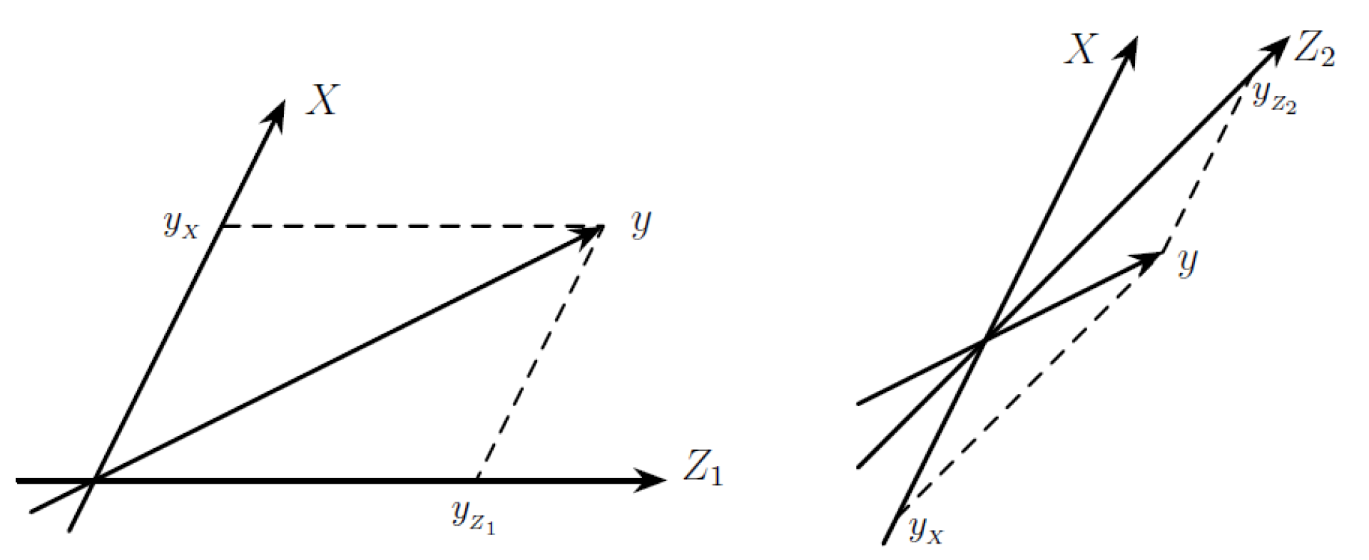
Figure 2.
Exact-identification accuracy by number of irrelevant features, with
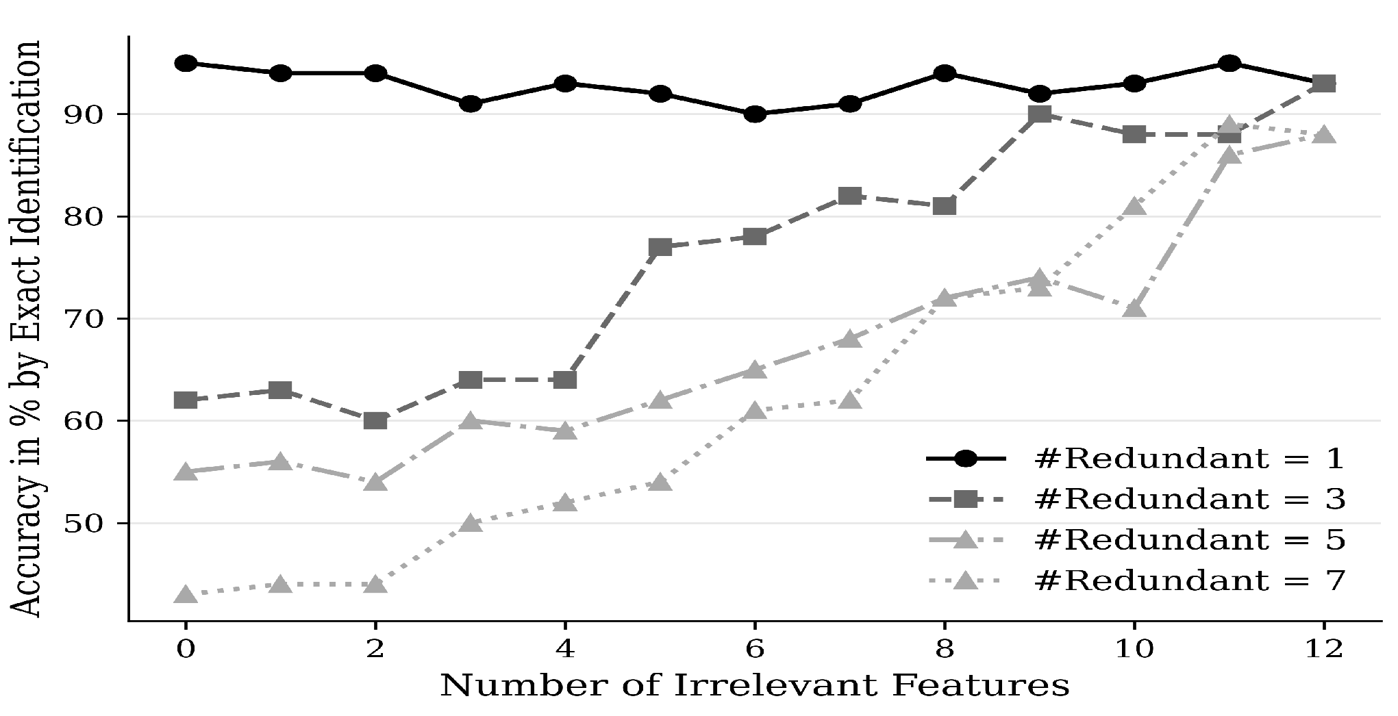
Figure 3.
Exact-identification accuracy by number of redundant features, with
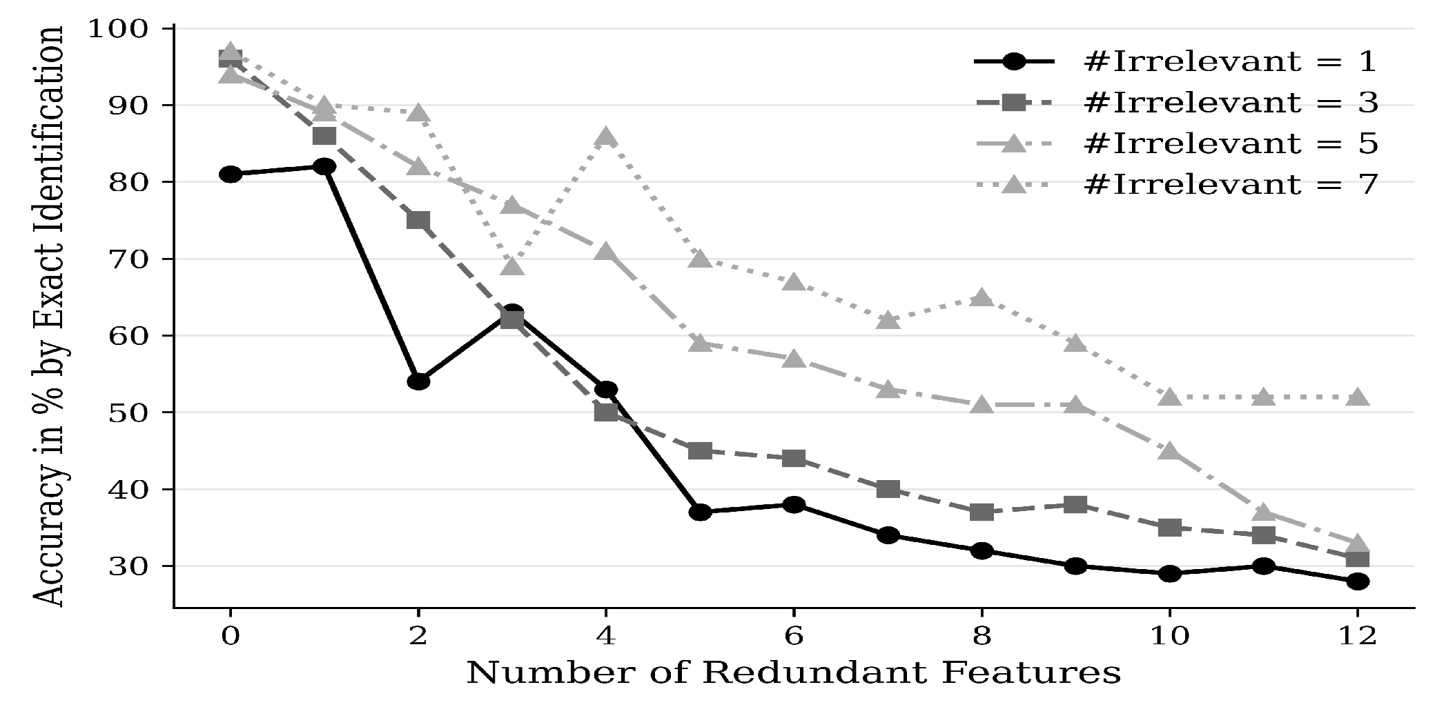
Figure 4.
Exact-identification accuracy by number of essential features, with five redundant features
Figure 4.
Exact-identification accuracy by number of essential features, with five redundant features
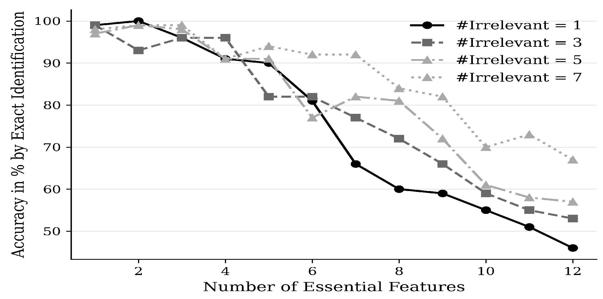
Figure 5.
Exact-identification accuracy by number of essential features, with five irrelevant features
Figure 5.
Exact-identification accuracy by number of essential features, with five irrelevant features
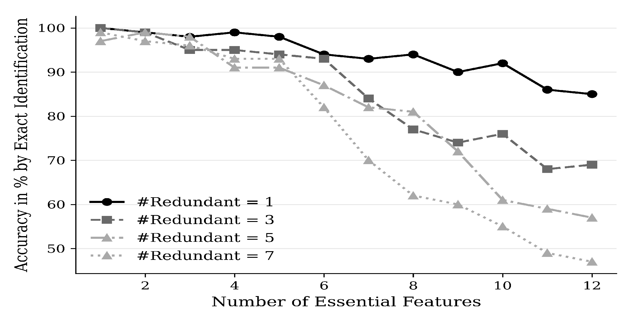

Table 1.
Average accuracy across 20,000 simulated datasets.
| Method | Stepwise | Unidirectional | Swapwise | GETS | LASSO | Algorithm 1 |
|---|---|---|---|---|---|---|
| 3.455% | 4.120% | 2.105% | 3.325% | 4.210% | 73.560% | |
| 5.485% | 6.180% | 4.310% | 6.065% | 8.085% | 88.620% |
Table 2.
Average underfit and overfit rates across 20,000 simulated datasets
| Stepwise | Unidirectional | Swapwise | GETS | LASSO | Algorithm 1 | |
|---|---|---|---|---|---|---|
| Underfit Rate | 30.23% | 28.92% | 34.71% | 30.51% | 20.83% | 7.12% |
| Overfit Rate | 34.17% | 29.36% | 38.26% | 33.92% | 23.61% | 8.47% |
Table 3.
Number of exact matches between and among 100 replications, by sample size
| sample size (100 simulated datasets per design) | ||||||||||
|---|---|---|---|---|---|---|---|---|---|---|
| 100 | 150 | 500 | 1,000 | 5,000 | 10,000 | 50,000 | 100,000 | 1,000,000 | ||
| .05 | .05 | .04 | .03 | .01 | .005 | .001 | .0005 | .0001 | ||
| 86 | 90 | 93 | 96 | 98 | 98 | 98 | 99 | 100 | 100 | |
| 53 | 66 | 83 | 87 | 91 | 93 | 94 | 96 | 99 | 99 | |
| 58 | 69 | 79 | 82 | 84 | 91 | 94 | 97 | 99 | 100 | |
| 34 | 49 | 56 | 65 | 68 | 78 | 82 | 89 | 94 | 97 | |
| 48 | 55 | 69 | 81 | 85 | 87 | 91 | 93 | 95 | 97 | |
Disclaimer/Publisher’s Note: The statements, opinions and data contained in all publications are solely those of the individual author(s) and contributor(s) and not of MDPI and/or the editor(s). MDPI and/or the editor(s) disclaim responsibility for any injury to people or property resulting from any ideas, methods, instructions or products referred to in the content. |
© 2026 by the authors. Licensee MDPI, Basel, Switzerland. This article is an open access article distributed under the terms and conditions of the Creative Commons Attribution (CC BY) license (http://creativecommons.org/licenses/by/4.0/).
Copyright: This open access article is published under a Creative Commons CC BY 4.0 license, which permit the free download, distribution, and reuse, provided that the author and preprint are cited in any reuse.