
Submitted:
11 November 2026
Posted:
12 November 2026
You are already at the latest version
Abstract
Treatment interruption and restart require assessment of patient recovery, delayed toxicity, and disease response. This study presents a focused application of Longitudinal Optimization of Global Outcomes and Strategies (LOGOS), to three methodological tasks: a) evaluating predictive information available before restart, b) comparing delayed effects across complete dosing schedules with specified administered amounts and follow-up, and c) examining how recovery mechanisms alter modeled disease control and injury. Exploratory clinical analyses were kept separate from pharmacokinetic/pharmacodynamic (PK/PD) and hypothetical simulations. Among 132 recorded mercaptopurine restart episodes from 73 patients, pre-restart absolute neutrophil count (ANC) improved internal prediction of the minimum ANC recorded within 14 days after restart (patient-weighted leave-one-patient-out RMSE reduction: 7.33%). Palbociclib PK/PD simulations yielded different ANC nadirs despite equal total administered amounts and follow-up. Hypothetical mechanistic simulations identified conditions under which cycling improved modeled disease control while reducing injury. Abiraterone analyses described PSA trajectories during biomarker-guided interruption and restart but did not establish restored drug sensitivity. The LOGOS’s methodological contribution refers to structure restart-time prediction and full-course schedule comparison under explicit conditions, not to introduce new PK/PD equations. Potential clinical applications include post-restart monitoring support and comparative treatment planning; clinical benefit remains unproven and requires external validation and prospective evaluation.
Keywords:
LOGOS framework
; dosage regimen scheduling
; treatment interruption and restart
; recovery dynamics
; pharmacokinetic/pharmacodynamic modeling
; clinical prediction
; delayed toxicity
1. Introduction
Treatment optimization requires attention to dose, timing, interruption and restart. Exposure may persist after dosing stops, while marrow responses can lag because of biological turnover [1,2] and recovery during a gap therefore need not predict post-restart toxicity. In childhood acute lymphoblastic leukemia (ALL), mercaptopurine adherence and thiopurine exposure are linked to relapse risk [3,4], whereas withholding may be required for hematological toxicity. Jost et al. [5] modeled absolute neutrophil count (ANC) from clinical blood counts and recorded 6-mercaptopurine (6MP) dosing and simulated maintenance regimens. However, their study did not specifically test whether ANC measured just before a recorded restart improves prediction of the subsequent observed minimum beyond earlier measurements. Gaps between dose records cannot establish ingestion or intentional withholding.
Interruption may also affect disease response. Adaptive therapy considers interactions between sensitive and resistant cells [6], and prostate-specific antigen (PSA)-guided abiraterone has been investigated clinically [7,8]. Zhang et al. [8,9] analyzed biomarker-triggered switching and clinical outcomes, but selected PSA trajectories do not themselves demonstrate restored drug sensitivity at matched exposure. Experimental drug-dependence findings [10] cannot be generalized across diseases: intermittent androgen deprivation met an overall-survival noninferiority criterion after radiotherapy [11], whereas noninferiority was not established in metastatic hormone-sensitive disease [12]. For toxicity, marrow-turnover models [13] and the palbociclib pharmacokinetic/pharmacodynamic (PK/PD) analysis [14] already capture delayed neutrophil responses, although this does not establish equivalent clinical effects across schedules. Furthermore, enhanced OptiDose [15] optimizes doses and dosing intervals under efficacy and safety constraints. The gap addressed here is therefore not an absence of timing-aware methods, but the need for explicit restart-time prediction and full-course schedule comparisons under defined conditions, with clinical observations and simulations interpreted separately.
Longitudinal Optimization of Global Outcomes and Strategies (LOGOS) has been proposed for assessing therapeutic strategies under common objectives, resource requirements and safety constraints [16]. The present LOGOS Theory A application specifies the restart landmark, outcome window, administered amount, initial state, residual exposure and follow-up where relevant to each analysis. This is a structured approach to evaluating interruption and restart, not a new PK/PD model, a replacement for existing dose-interval optimization methods, or a clinically validated dosing algorithm.
This study has four objectives: a) to evaluate whether pre-restart ANC adds information for predicting the minimum recorded ANC within 14 days after 6MP restart, b) to compare delayed neutropenia in palbociclib PK/PD simulations of schedules with matched total administered dose and follow-up, c) to examine, in a hypothetical mechanistic model, conditions under which cycling changes modeled disease control and injury, and d) to describe PSA trajectories during biomarker-guided abiraterone interruption and restart. The 6MP analysis is the primary clinical prediction component. The PSA analysis is secondary and descriptive, and neither simulation component validates the clinical findings.
2. Materials and Methods
2.1. Study Design
Retrospective secondary analyses of clinical data were combined with separate mechanistic simulations. All clinical analyses were exploratory and post hoc. Further diagnostic and sensitivity checks were utilized. The primary analysis concerned internal prediction of the minimum recorded ANC strictly after restart and through day 14. Changes in ANC during the gap, matched comparisons with intervals without a gap, and PSA analyses were used to examine related clinical questions. The simulations addressed specified mechanisms and toxicity comparisons as they were not fitted to the restart episodes and therefore did not provide validation cohorts for the ANC model. The essential clinical definitions and prediction coefficients are given in Appendix A, and the pharmacological comparison details in Appendix B. Section 2.5 presents the core mechanistic equations. Extended clinical results are in Tables S1–S12 and Figures S1–S3, mechanistic parameters and checks in Tables S13–S28 and Figures S4–S5, and palbociclib equations, exposure summaries and input hashes alongside Tables S29–S30. Terminology follows the data source: a recorded dose-event gap denotes an interval between 6MP records, while an observed OFF episode denotes visit-recorded abiraterone status, a simulated OFF period denotes zero administered input in a model and does not imply zero exposure.
Figure 1 shows the four analytical components of the study and their research questions. Table 1 describes how observed clinical measurements differ from simulated and hypothetical model quantities and what are their principal interpretive limitations. These components address complementary aspects of interruption and restart but do not validate each other.
2.2. ALL Records and Definition of Restart Episodes
The data were obtained from Data Sheet 2 accompanying Jost et al. [5]. The file contained 55,305 event records from 116 patients, comprising 5,897 ANC measurements and 49,408 dose records for 6MP. Observed ANC values, expressed in G/L, were used throughout the analysis. Historical model predictions were excluded from the outcomes so that the comparison would refer to measured blood counts. Related gap-selection checks and source-input hashes are reported in Tables S1–S3 and S30. The source study concerned childhood ALL maintenance at two German centers [5]. Age, sex, calendar recruitment dates, hospital identifiers and exact clinical TIME zero were not available in this released event file. Body size at the pre-restart anchor is summarized in Table S8, while source-cohort demographics cannot be assigned to the selected 73 patients.
A recorded dose-event gap was identified when consecutive dose records were more than 1.50 days apart. Its start was one day after the preceding dose and its end was the next recorded dose, defining recorded restart. Eligibility required a gap of at least 2.99 days. A three-day criterion with tolerance for floating-point arithmetic selected the same episodes (Table S2). This definition does not establish intentional withholding, adherence or washout. For example, consecutive dose times 69.79 and 81.79 days give gap start 70.79 and duration 11.00 days (Appendix A). Pre-gap ANC was the latest nonnegative recorded measurement in the seven days ending at gap start. Pre-restart ANC was the latest such measurement within the gap and within seven days before recorded restart. The latter had to follow the pre-gap measurement (no interpolation was used). Valid recorded zeros were retained. The outcome was the minimum ANC recorded strictly after restart through day 14. Episodes without an observed outcome were excluded. A separate analysis required at least two follow-up counts, and another used the count nearest day 7 within days 5–9 (Appendix A, Tables S1–S5 and S11).
ANC changes during the gap were also examined, including a subgroup with baseline ANC below 0.50 G/L. For within-patient comparisons, intervals without a recorded dose gap were matched on baseline ANC, measurement spacing, preceding dose intensity and treatment timing. The 0.50 G/L boundary served only to define this descriptive subgroup. Dose was normalized by body surface area. Weekly methotrexate was part of the source treatment setting, but its administration was unavailable, together with adherence, infection status, reasons for interruption and C-reactive protein. Consequently, the inflammation-related exclusions used in the original study could not be reproduced.
2.3. ANC Prediction and Statistical Assessment
Two ordinary least-squares (OLS) models used identical complete cases. The baseline model contained pre-gap ANC, restart dose in mg/m², gap duration and restart TIME in source-recorded days. The enhanced model added pre-restart ANC, while both included an intercept and linear additive terms. TIME was not recentered. Its precise clinical origin was not documented, so the coefficients require the original time coordinate. Predictions are conditional on the selected restart dose and subsequent care as practiced. Dose was removed in a sensitivity analysis. A separate reduced association model adjusted only for pre-gap ANC and restart dose. All eligible complete cases were used. No formal development sample-size calculation was undertaken. There were 37 patients with one episode, 20 with two, 12 with three, three with four and one with seven. The number of independent patient clusters, rather than 132 independent observations, governs the scope of internal evaluation.
The predictive performance of a model needs to be assessed separately from its fit to the data used for development [17]. In the present analysis, leave-one-patient-out (LOPO) evaluation was applied: all episodes belonging to one patient were excluded during fitting, and the fitted model was then used to predict that patient’s outcomes. The procedure was repeated for every patient. Prediction errors were averaged first within each patient and then across patients, giving equal importance to patients with different numbers of interruptions. Root mean squared error (RMSE) expresses error in G/L and places greater weight on large discrepancies, while mean absolute error (MAE) describes their average absolute magnitude. Calibration was used to assess agreement between predicted and recorded counts, together with error measures and a defined prediction setting [18,19]. The coefficients and calculation details are provided in Appendix A. Uncertainty was assessed with 2,000 bootstrap samples of whole patients. Both models were refitted in each sample, excluding every sampled copy of the patient being predicted. Patient-cluster bootstrap 95% percentile intervals were calculated for absolute error measures, paired error reductions and calibration. The ≥2-visit and no-dose analyses were retrained separately. These intervals describe internal performance in the source population, while no external or later cohort was available. Additional post hoc checks examined selection, measurement timing, visit frequency, dose changes, residual patterns, influential observations and patient deletion. LOPO predictions were repeated with recent anchors, a common follow-up window, exclusion of pre-restart ANC above 10 G/L and fixed Huber regression. No negative prediction was truncated. A separate follow-up model examined the observation process. These checks cannot recover an unmeasured low count or remove informative observation (Tables S3–S5 and S8–S11, and Figures S2–S3).
2.4. Palbociclib Simulation of Delayed Neutropenia
In PALOMA-3, neutropenia was a frequent adverse event managed through blood-count monitoring and dose interruption, delay or reduction [20]. To examine how these blood-count changes develop over time, the published palbociclib PK/PD model was reconstructed using typical parameter values [14]. The marrow compartments describe the delay between the drug effect on proliferating cells and the subsequent change in circulating neutrophils [13]. Clearance and feedback estimates reported in the source abstract were used in the principal reconstruction, with the final-table estimates assessed separately. Appendix B lists the parameter values, dose counts and follow-up details. The equations and numerical settings accompany Table S29 in the Supplementary Material.
The cycling schedule consisted of six cycles of 125 mg daily for 21 days followed by seven days without dosing. The 93.75 mg daily schedule was a hypothetical, non-clinical equal-total-oral-mass comparator. Both delivered 15,750 mg within 168 days, began with no drug and baseline blood-cell pools, and continued to day 182. ANC minima were sought throughout treatment and follow-up. These typical-parameter simulations contain no between-patient variability or cancer-control endpoint. Equal total oral mass does not establish equivalent exposure profiles or antitumor efficacy and does not support a dosing recommendation.
2.5. Exploratory Simulation of Recovery and Treatment Response
A separate hypothetical model was used to investigate whether recovery of a component of drug action could favor treatment cycling. Drug exposure was linked to available responsiveness, accumulated injury and disease burden. The model allows responsiveness to recover as exposure decreases, while disease can regrow during an interruption. This provides a means of examining the competing consequences of stopping and resuming administration. The states were not fitted to the clinical datasets: ANC was not used as a measure of responsiveness or injury, and PSA was not converted to model disease burden. The equations describe the assumptions used in the simulations and have no established application as a clinical dosing algorithm.
2.5.1. Model States and Their Interpretation
The model includes relative drug exposure C, the available fraction of treatment responsiveness R, accumulated injury Z and relative disease burden D. Administration is represented by the normalized input u. Time t is expressed in units of responsiveness recovery, without a fitted conversion to clinical days. Exposure and injury are nonnegative, disease burden is positive, and responsiveness ranges from zero to one. The corresponding equations are
Equation (1) links administration to exposure. Equation (2) balances restoration of responsiveness against depletion by drug effect. Equation (3) balances injury production against repair. In Equation (4), ρ[1−E(C)] represents an assumed cytostatic suppression of growth that remains independent of R, whereas ηE(C)R represents responsiveness-dependent killing. This separation is a modeling assumption. A structural sensitivity replaced the growth term by ρ[1−E(C)R]. Injury Z does not feed back into C, R or D. Changing injury repair therefore leaves disease control unchanged by construction. The functions in Equation (5) describe how exposure affects these processes. Drug effect E(C) increases with exposure and reaches one half at C=1. In contrast, the recovery functions W(C) and WZ(C) decrease as exposure rises. Their respective half-recovery levels are χ and χZ, while n determines the steepness of the change in responsiveness recovery. This formulation allows recovery to continue after administration stops, as residual exposure declines. The reference values were κ=4, α=2, β=0.20, π=0.70, η=1, ρ=0.08, χ=0.35, χZ=1, n=4 and s=1. These parameters and the injury thresholds are normalized quantities without fitted clinical equivalents.
2.5.2. Disease Control and Injury over the Complete Course
Disease control was assessed by the average rate of decline in modeled burden. For a repeating schedule, J is the cycle average of treatment effect minus disease growth, with angle brackets denoting that average. For a finite course, the treatment window H is followed by an untreated observation period L, and JF is calculated from the change in burden over the entire interval:
J = η⟨E(C)R⟩ − ρ⟨1 − E(C)⟩
Positive J or JF indicates declining modeled burden, zero stability and a negative value growth. These are not clinical response or survival rates. The highest Z was compared with stipulated model-injury constraints of 0.50 and 0.22. The former defines the reference feasibility screen, the latter examines a stricter constraint that can distinguish the simulated regimens. Neither threshold was estimated from toxicity data or corresponds to a clinical ANC boundary. For the repeated-cycle comparison, exposure, responsiveness and injury were initialized at their repeating C/R/Z state. Relative burden D was set to one and was then allowed to change, since a repeating exposure pattern does not require disease burden to be periodic. The constant comparator started at its stationary C/R/Z state. The finite-course comparison used the same initial state for both regimens, (C,R,Z,D)=(0,1,0,1), corresponding to no drug, full responsiveness, no injury and baseline burden. In this way, initiation and post-treatment effects were included in addition to the behavior observed during repeated cycles.
2.5.3. Equal Administered Input and Residual Exposure
The schedules were compared at a mean input q=1 over cycle length T. This was achieved by maintaining input one continuously or administering input 1/f during the active-dosing (ON) fraction f, with zero input during the remainder of the cycle. Integration of Equation (1) gives the relationship between administered input and exposure over the treatment window. When input is stopped at H, the exposure remaining beyond the end of follow-up H+L can also be calculated:
The principal periodic candidate had T≈1.68 and f=0.20, with ON input five. It was selected from 1,395 screened period–duty combinations followed by local refinement (Tables S14 and S28, Figure S4). For the finite course, continuous input one for H=20 was compared with 12 cycles of length 20/12 at the same ON fraction and intensity. Both delivered 20 model units and were followed without input for L=5. Equations (9) and (10) retain exposure at the observation boundaries. Equal normalized input represents equal administered mass only with common bioavailability, clearance and concentration scaling.
Fixed-schedule structural controls and parameter sensitivities examined restoration, depletion, regrowth, injury production, repair and exposure timescale. Periodic timing was screened over 1,395 period–duty combinations, finite timing used 24 equal-input schedules. Ranges were selected as illustrative perturbations, not clinical uncertainty intervals. The Supplementary Material summarizes the parameter and structural checks, screened schedules, candidate identities and numerical balances (Tables S13–S28, Figures S4–S5). These calculations do not identify a clinically optimal interval.
2.6. Secondary Descriptive PSA Analysis
Adaptive abiraterone records were used only to describe PSA changes under biomarker-triggered switching [8,9]. Completed OFF episodes, restart landmarks and adjacent ON slopes followed separate eligibility rules. The primary descriptive slope contrast was the median of patient-specific median contrasts, while the episode-weighted estimate was secondary. This priority was chosen post hoc. Supplementary Tables S6–S7 and S12 and Figure S1 summarize OFF episodes, selected landmarks, adjacent-ON contrasts and eligibility differences. No exposure-matched responsiveness or comparative efficacy analysis was possible.
2.7. Uncertainty and Reproducibility
Descriptive clinical intervals used 2,000 patient-cluster bootstrap samples, with one median per patient for patient-weighted summaries. These exploratory intervals were not adjusted for multiple comparisons and cannot eliminate selection or confounding. Bootstrap specifications and seeds are provided in Appendix A, with full-retraining error and calibration intervals in Tables S5 and S9–S10. Each treatment switch and dose event was represented explicitly in the simulations, and extrema were evaluated over the complete trajectories, including times between stored observations and post-treatment follow-up. Numerical accuracy was assessed through independent calculations and drug-amount accounting (Tables S15–S16 and S28–S29), while the palbociclib integration settings accompany Table S29.
2.8. Computational Implementation
All data processing, statistical analyses and numerical simulations were performed using Python (v. 3.12). The computational environment included NumPy (v. 2.5.2) for numerical calculations, pandas (v. 3.0.5) for data manipulation, statsmodels (v. 0.15.0) for ordinary least-squares regression, scikit-learn (v. 1.9.0) for prediction evaluation and error metrics, SciPy (v. 1.18.1) for numerical integration and optimization, and Matplotlib (v. 3.11.1) for visualization. Study-specific scripts implemented the statistical workflows and PK/PD and mechanistic simulations. Their numerical settings, dependencies and random seeds are documented in the computational Supplementary Material.
3. Results
3.1. ANC Eligibility and Internal Prediction
Selection identified 803 recorded dose-event gaps in 107 patients, including 338 eligible gaps in 102 patients. Of these, 170 lacked a pre-restart anchor and 27 further episodes lacked a pre-gap anchor. None failed only because of reversed anchor order. The remaining 141 pairs involved 74 patients. Nine had no post-restart count, 19 had one, 112 had two and one had three. Prediction therefore used 132 episodes in 73 patients, or 39.05% of eligible gaps. The ≥2-visit analysis used 113 episodes in 63 patients (Figure 2).
The pre-restart measurement preceded restart by a median 0.37 days (interquartile range 0.37–1.37, range 0.37–6.37). The first subsequent count occurred at median day 6.63 and the recorded minimum at day 7.13. The included episodes had median gap duration 7.00 days, pre-gap ANC 1.84 G/L and pre-restart ANC 1.75 G/L. The 206 excluded episodes had fewer follow-up counts and substantial anchor nonavailability (Supplementary Table S8). No 14-day outcome windows overlapped within a patient. Across the ordered pairs, the median ANC change was −0.20 G/L (95% interval −0.45 to 0.20), and an increase was observed in 45.4% of episodes. The low-baseline subgroup included 16 episodes in 12 patients, with a median change of 0.85 G/L (0.50–1.85). Only three target episodes could be matched to an interval without a gap in the same patient. Their differences-in-change were −1.11, 0.20 and 3.10 G/L. These few, opposing contrasts were insufficient for a stable causal assessment of withholding treatment.
Higher pre-restart ANC was associated with a higher recorded minimum after restart. In the reduced adjusted model, the coefficient was 0.24 G/L per G/L (0.14–0.38), and 0.24 after rounding in the full five-predictor OLS model. The unrounded estimates differ because the full model includes additional predictors. Restricting the lag of the pre-restart measurement to ≤1.50 days retained 121 episodes in 66 patients and gave a reduced-model coefficient of 0.23 (0.12–0.38). Positive associations were also obtained after patient weighting and retrospective adjustment for sampling characteristics (Table S4). Adding pre-restart ANC reduced patient-weighted LOPO RMSE from 0.93 to 0.86 G/L and MAE from 0.63 to 0.57 G/L (Table 2, Figure 3). The RMSE reduction was 0.07 G/L, or 7.33%, calculated from unrounded values. Paired reduction in mean squared error (MSE) was 0.12 (G/L)² (patient-cluster bootstrap 95% percentile interval 0.0047–0.28), i.e., the lower bound was close to zero. The MAE-reduction interval included zero (−0.01 to 0.13 G/L). Forty-nine of 73 patients had lower squared error. With ≥2 visits, RMSE was 0.92 versus 0.85 G/L, but the MSE-reduction interval included zero (−0.0020 to 0.32). These are exploratory internal estimates, not reductions in toxicity.
RMSE and MAE are in G/L, while paired MSE reduction is in (G/L)². Positive reductions favor the enhanced model. Intervals are exploratory patient-cluster bootstrap 95% percentile intervals with full model retraining. The no-dose analysis removes dose from both models. Full coefficients and descriptive associations are in Tables A1 and Table A2, while absolute-error, paired ΔRMSE/ΔMAE and calibration intervals are in Tables S9–S10. Differences and percentages use unrounded values. The held-out calibration intercept/slope was 1.10/0.34 for baseline and 0.31/0.83 for enhanced predictions. Uncertainty remained substantial (Table S10). Figures S2–S3 present calibration and residual diagnostics, respectively. The no-dose comparison retained a favorable MSE estimate, and recent-anchor, day-7-window, Huber and high-ANC checks retained the direction of the RMSE change (Table S11). Follow-up-frequency models did not improve on the reference and had optimizer warnings. This does not demonstrate independent monitoring. Only five minima were below 0.50 G/L, insufficient for a stable severe-neutropenia threshold.
3.2. Palbociclib Exposure and Delayed Marrow Response
The modeled ANC nadirs were 1.13 G/L during cycling and 1.35 G/L with hypothetical daily redistribution, at days 52.46 and 39.06, respectively (Figure 4, Table 3). Both occurred before the end of dosing. The 14-day post-treatment tail did not lower either global nadir. Final-table clearance and feedback values gave nadirs of 1.14 and 1.36 G/L. This ordering applies to these two specified typical parameters sets and does not estimate probabilities of severe neutropenia. Equal total oral mass produced different exposure profiles: peak concentrations were 104.58 and 78.43 µg/L, and area under the concentration–time curve (AUC) through day 168 was 11,494.81 and 11,432.29 µg·day/L for cycling and daily dosing, respectively. The infinite-horizon AUC was identical under the shared linear pharmacokinetic model (Table S29). Thus, daily intensity and interruption jointly determine the comparison. It does not isolate a holiday effect or establish equal cancer control.
These are typical-parameter simulations with no statistical uncertainty interval or antitumor endpoint. The final-table sensitivity uses clearance 57.13 L/h and feedback exponent 0.103. Appendix B gives full parameter and dose details. The daily regimen is a hypothetical non-clinical comparator. The ranking is restricted to these specified parameter sets.
3.3 Mechanistic Conditions for a Benefit from Cycling
The hypothetical model produced different disease trajectories under continuous and cyclic administration despite equal average input. Modeled burden increased with continuous administration and declined with the selected cycle, with disease-control rates of −0.03 and 0.08 per model time unit, respectively. Peak injury was 0.29 for continuous administration and 0.19 for cycling. Both were below the reference threshold of 0.50 (Table 4).
The comparison from treatment initiation gave the same qualitative result. Starting from identical states and administering the same total amount, continuous treatment resulted in a final burden of 1.72 times baseline, compared with 0.25 for cycling. Peak injury over the course was 0.29 and 0.19, respectively. The small amount of exposure remaining beyond follow-up was retained in the accounting. Figure 5 presents the time course of recovery, disease burden and injury for these comparisons.
Positive J or JF denotes declining modeled burden. Periodic comparisons use each model’s periodic state. Finite comparisons start before administration and include follow-up. Input and injury thresholds are normalized, without clinical equivalents. Fixed-schedule structural results are in Tables S23–S24, while screened structural and repair-gating checks are in Tables S17–S18. Feasibility refers only to the stipulated model-injury constraint. This provides a mechanistic counterexample under specified assumptions, rather than evidence of clinical superiority. Holding responsiveness at one or disabling restoration removed the cycling advantage both in the fixed-schedule controls and in the screened comparisons. Making repair exposure-independent changed injury but could not change disease control, because Z has no feedback into the other states. The alternative growth term ρ[1−E(C)R] retained the direction of the fixed-schedule comparison (Tables S23–S24). The screened stricter-constraint comparison and the reference locally refined trajectory are distinct runs (Tables S14 and S28).
Across the repeated-cycle grid, 54 of 1,395 candidates had no positive control-rate gain over constant input, and 173 exceeded the stipulated 0.50 injury cap. The fixed reference cycle retained a higher J across the 18 one-factor scenarios, but at ρ=0.32 its J was −0.07 and modeled burden still increased. All 24 finite timing scenarios retained a positive JF difference, ranging from 0.0019 to 0.08, while peak cyclic injury ranged from 0.18 to 0.30. Thus, a relative advantage does not ensure declining burden, lower injury or feasibility under every constraint (Tables S25–S27, Figures S4–S5).
3.4 Secondary PSA Observations
There were 53 completed OFF episodes in 17 adaptive-treatment patients and three terminal censored intervals. PSA increased in every completed episode, conditional on the PSA-triggered restart rule. The strict restart landmark included 27 episodes in 14 patients, while the separate adjacent-ON analysis included 13 pairs in eight patients. Its primary patient-weighted slope contrast was +0.0104/day (95% percentile interval −0.0189 to 0.0190), and the secondary episode-weighted contrast was +0.0147/day (0.0034–0.0184). Positive contrasts indicate slower subsequent decline. Selected outcomes, eligibility comparisons and timing sensitivities are summarized in Tables S6–S7 and S12 and Figure S1. These observations do not establish restored drug sensitivity.
4. Discussion
4.1. Prediction of ANC After Treatment Restart
The principal clinical finding concerns internal prediction of the recorded ANC minimum after 6MP restart. Whereas Jost et al. [5] modeled longitudinal ANC dynamics during ALL maintenance and explored dosing regimens, the present analysis asks whether the latest pre-restart ANC adds predictive information beyond pre-gap ANC, dose and timing at a defined restart landmark. The methods and endpoints differ, so the observed prediction improvement is not evidence of superiority over the earlier PK/PD approach. PSA observations, palbociclib PK/PD simulations and hypothetical mechanistic simulations concern different drugs, endpoints and evidence types. They neither cross-validate the ANC finding nor provide a common estimate of clinical efficacy or safety. Favorable point estimates persisted across sensitivity analyses, but the ≥2-visit MSE interval and the primary MAE-reduction interval included zero. These predictions describe outcomes under observed care as they do not establish effects of raising ANC, prolonging an interruption or changing dose.
The sampling schedule is central to the interpretation of this result. When only one post-restart count is available, that measurement becomes the minimum by definition. With two measurements, there are two opportunities to observe a lower count. Requiring two visits therefore changes both the information available and the patients represented, while any lower value between visits remains unknown. Calibration and the magnitude of the prediction errors also need to be considered: a lower average error does not compensate for systematic disagreement between predictions and observations in the intended population [19]. In the present data, persistence of ANC over time, clinical dose selection, concurrent therapy and selective monitoring can all contribute to the observed association. The increase observed in the low-baseline subgroup addresses a different question. Selection on a low initial value permits regression to the mean, and the three available within-patient matches were insufficient for a stable causal comparison. Thus, the descriptive change during interruption cannot be interpreted as the effect of withholding 6MP.
Zhang et al. [8,9] investigated biomarker-guided adaptive abiraterone and reported clinical outcomes in their study population. In contrast, the present reanalysis is limited to descriptive OFF/ON PSA landmarks, with substantial uncertainty in the patient-weighted slope contrast and unequal segment durations and starting PSA values (Table S12). A post-restart PSA decline indicates on-treatment activity within these selected segments. It neither independently establishes comparative efficacy nor demonstrates restored drug sensitivity at matched exposure.
4.2. Exposure and Delayed Toxicity During Treatment Cycling
Le Marouille et al. [14] fitted a population PK/PD model to palbociclib concentrations and ANC observed in patients, including between-patient variability. The present reconstruction instead applies published typical parameters to two specified schedules with equal total oral mass. It addresses a schedule-comparison question rather than validating or improving that population model. Although ANC rose during dosing interruptions, the simulated global nadir for cycling was lower than for the hypothetical daily comparator. Daily intensity, residual exposure and delayed marrow response contribute together. The contrast therefore does not isolate a drug-holiday effect. Neither antitumor efficacy nor variability-based risk was modeled, so the comparison cannot justify changing clinical dosing. PALOMA-3 [20] supports monitoring and protocol-directed management of neutropenia, not the hypothetical comparator examined here. In the separate mechanistic model, recovery of responsiveness can alter the balance between drug action and regrowth, but that outcome depends on stipulated biological processes. The reference growth law includes a cytostatic component independent of responsiveness. An alternative law retained the qualitative fixed-schedule contrast without clinical calibration. Injury has no feedback into disease control, so modifying repair cannot improve modeled burden by construction. Some screened schedules offered no relative advantage, and greater regrowth could leave both regimens with increasing burden. Relative modeled control and feasibility under injury constraints must therefore be considered jointly.
Even when total administered amount and follow-up are matched, concentrations and finite-window exposure can differ between schedules. Initial conditions and post-treatment observation can also change the assessed extrema (Section 2.5). Enhanced OptiDose [15] explicitly optimizes dosing amounts or intervals under efficacy and safety constraints. The present study does not solve such an optimization problem or identify a clinically optimal cyclic regimen. Rather, its matched-input and full-follow-up comparisons clarify which differences arise under the specified schedules. Equal oral mass alone does not establish equal exposure, antitumor efficacy or clinical safety.
4.3. Prediction and Restart Decisions
An improvement in prediction becomes clinically useful only if it informs a decision with a favorable balance of outcomes. The ANC analysis compared the information available for prediction while keeping the observed treatment decisions fixed. Evaluation of an ANC-informed restart strategy would additionally require a defined decision time, the actions available at that time, toxicity and disease outcomes, and a method for handling subsequent dose adaptation. Monitoring and dose resources would also need to be comparable between strategies. Decision-curve analysis provides a means of evaluating net benefit across specified decision thresholds [23], but no decision-curve, net-benefit or policy-effect analysis was performed in this study.
A further step concerns the relationship between the clinical measurements and the hypothetical model states. ANC cannot simply replace responsiveness or injury, nor can PSA be treated as an exact measure of modeled burden. Such use requires a calibrated relationship between the measurements and the underlying processes, supported by exposure data and assessment of parameter identifiability [24]. A comparison of a state-informed strategy with restart on a fixed day would then need explicit eligibility criteria, strategies, follow-up and a causal contrast, as in a target-trial specification [25]. Before this comparison, external or temporal evaluation should establish whether the ANC association extends beyond the present prescribing and monitoring process. Drug-specific PK/PD calibration would be required for clinical interpretation of any subsequent policy simulation.
4.4. Limitations
The retrospective, post hoc design places several restrictions on interpretation. Actual exposure and adherence were unavailable, as were reasons for interruption, methotrexate administration, infections and inflammation. The effect of 6MP withholding therefore cannot be isolated from the combined ALL maintenance treatment. This is particularly relevant in view of the prospective studies linking adherence and thiopurine exposure to relapse [3,4]: recorded dose events do not provide the same information as drug intake or systemic exposure. Sparse ANC sampling and potentially selective missing outcomes further restrict assessment of the lowest count. In the PSA analysis, biomarker-triggered switching selected small subsets with unequal segment duration. Resampling intervals quantify uncertainty within these data but do not remove the restrictions imposed by their collection. Restart-dose amounts subsequently changed within 14 days in 57 of 132 episodes. These future changes were not primary predictors. The model therefore describes observed post-restart care rather than a fixed-dose intervention. In addition, the ANC model was developed and internally evaluated in a selected subset of one source collection, with 73 independent patient clusters and five predictors plus an intercept. No formal sample-size calculation or external validation supported this exploratory development. Age and sex were absent from the released records, precluding demographic performance comparisons. LOPO estimates performance for another patient from the same collection, not a new hospital or prescribing policy. Calibration uncertainty, influential episodes and missing outcomes remain relevant. The 7.33% RMSE reduction has not been linked to fewer infections, treatment delays or severe neutropenic events. Typical-parameter and uncalibrated simulations cannot supply that evidence.
4.5. Methodological Novelty and Potential Clinical Applications
Established PK/PD approaches already model neutrophil turnover and dosing effects [5,13,14], and constrained methods already optimize doses and dosing intervals [15]. LOGOS Theory A therefore makes a narrower methodological claim. It organizes treatment interruption and restart around three distinct evaluations: a) whether information available at restart improves prediction beyond earlier measurements and recorded treatment history, b) how delayed toxicity differs across complete schedules when administered amounts, initial conditions and follow-up are specified, and c) under which hypothetical recovery mechanisms intermittent administration changes modeled disease control and injury. The contribution is the restart-focused analytical structure and explicit comparison conditions, not the discovery of treatment timing, new regression or PK/PD equations, or proof of clinical benefit. Clinical records and simulations remain distinct forms of evidence and do not validate one another. Clinical applications can refer to: a) using recovery measurements to support post-restart risk assessment and planning of hematological monitoring, b) assessing delayed toxicity after interruption, resumption and completion of dosing, and c) comparing candidate schedules in terms of expected efficacy, safety and drug requirements over a common observation period. These are proposed uses, not demonstrated improvements in clinical decisions or patient outcomes. Implementation would require external prediction validation, drug-specific calibration, explicit decision thresholds and prospective evaluation.
Study-specific computational scripts, settings and results are provided in the computational Supplementary Material, while related LOGOS implementations are available on GitHub [21,22]. These resources support reproducibility and methodological development but do not provide external clinical validation.
5. Conclusions
LOGOS Theory A provides a structured way to assess information available at treatment restart and to compare delayed effects of alternative dosing schedules over defined treatment and follow-up periods. In exploratory 6MP records, pre-restart ANC improved internal prediction of the recorded post-restart minimum. Separate palbociclib and hypothetical simulations illustrated schedule-dependent neutropenia and mechanisms that can change modeled disease control and injury. PSA analyses described biomarker-guided switching without establishing restored sensitivity. These findings motivate three potential uses such as restart-time risk assessment, monitoring of delayed toxicity and comparative evaluation of dosing schedules. External validation, drug-specific calibration and prospective assessment of clinical decisions and outcomes are required before implementation.
Supplementary Materials
The following supporting information can be downloaded at the website of this paper posted on Preprints.org. The accompanying supplement contains Tables S1–S30 and Figures S1–S5. Clinical ANC and PSA analyses are presented in Tables S1–S12 and Figures S1–S3. Mechanistic-model parameters, comparisons and numerical checks in Tables S13–S28 and Figures S4–S5. Palbociclib exposure results and input-file hashes in Tables S29–S30. The palbociclib equations and numerical settings appear adjacent to Table S29.
Author Contributions
V.D.K. is the sole author of this work.
Funding
This research received no external funding.
Institutional Review Board Statement
This study presents mathematical models and numerical simulations. No participants were recruited, no intervention was administered and no new patient observations were collected.
Informed Consent Statement
Not applicable.
Data Availability Statement
The clinical data used in this study were from previously published and publicly available sources. The mercaptopurine and absolute neutrophil count (ANC) data from patients with acute lymphoblastic leukemia were obtained from Data Sheet 2 of Jost et al. [5] (https://doi.org/10.3389/fphys.2020.00217). The PSA data from adaptive abiraterone-treated patients were from the publicly available TrialPatientData.xlsx dataset in Zhang et al.’s GitHub repository [8,9] (https://doi.org/10.7554/eLife.76284; https://github.com/cunninghamjj/Evolution-based-mathematical-models-significantly-prolong-response-to-Abiraterone-in-mCRPC). The palbociclib PK/PD simulations were based on published model equations and parameter estimates from Le Marouille et al. [14] (https://doi.org/10.3390/pharmaceutics13101708). Computational implementations of the LOGOS framework are publicly available on GitHub (https://github.com/vkaralis/LOGOS-theory-A and https://github.com/vkaralis/LOGOS-theory-A-apps) [21,22]. Study-specific computational scripts, numerical settings and supporting results are provided in the accompanying Supplementary Material.
Acknowledgments
The author would like to express his gratitude to Professor Georgia Karali, Professor of Mathematics at the Mathematics Department of the National and Kapodistrian University of Athens, for her valuable scientific discussions, insightful suggestions, and constructive guidance regarding the mathematical formulation, analytical development, and solution of the mathematical models underlying the LOGOS theory. During the preparation of this manuscript, the author used Grammarly (accessed in October 2026) for language editing and clarity improvements. The author has reviewed and edited the content of this publication
Conflicts of Interest
The author declares no conflicts of interest.
Abbreviations
ALL, acute lymphoblastic leukemia; ANC, absolute neutrophil count; AUC, area under the concentration–time curve; LOPO, leave-one-patient-out; MAE, mean absolute error; MSE, mean squared error; OLS, ordinary least squares; PK/PD, pharmacokinetics/pharmacodynamics; PSA, prostate-specific antigen; RMSE, root mean squared error; 6MP, 6-mercaptopurine.
Appendix A Clinical Definitions and ANC Prediction
A1 Timing and Interpretation of Measurements
The endpoint is the minimum ANC recorded strictly after restart and within 14 days, not the continuous-time nadir. ANC in G/L is equivalent to 10⁹ cells/L. A recorded dose-event gap starts one day after the preceding dose and ends at the next dose record. For example, dose times 69.79 and 81.79 give a gap start of 70.79 and duration 11.00 days. Eligibility uses ≥2.99 days; the three-day sensitivity allows a 10⁻⁹-day numerical tolerance (Table S2). No ingestion or treatment-hold intention is inferred.
The pre-gap anchor is the latest nonnegative ANC in the seven days ending at gap start. The pre-restart anchor is within the gap, no more than seven days before restart and strictly later than the pre-gap anchor. Recorded zeros are valid under the source observation flags. No interpolation is used. Predictor-age and outcome-visit summaries are reported in Section 3.1 and Tables S3 and S8.
Among 141 episodes with ordered measurements, nine had no follow-up count, 19 had one, 112 had two and one had three. Exclusion of episodes without an outcome left 132 episodes in 73 patients for prediction. The requirement for at least two measurements retained 113 episodes in 63 patients. When only one value is available, it serves as the minimum. The sensitivity requiring two visits increases the number of opportunities to record a low count, but still cannot identify a lower value between visits.
A2 Prediction Inputs and Reproducible Coefficients
The baseline model contains pre-gap ANC, restart dose in mg/m², gap duration and un-recentered source TIME at restart. The enhanced model adds pre-restart ANC. The prediction is the intercept plus the sum of predictor–coefficient products. Table A1 retains precision for reconstruction; the machine-readable coefficients are in the revision package. Using another time origin requires a corresponding intercept adjustment. Table 2 performance comes from patient-excluded fits, not these full-sample fitted values.

Table A1.
Full-sample coefficients for reconstruction of the ANC prediction models.
| Predictor | Units | Baseline | With pre-restart ANC |
|---|---|---|---|
| Intercept (intercept) | G/L | 1.21635365971 | 0.763683340176 |
| Pre-gap ANC (pre_gap_ANC) | G/L per G/L | 0.0554696452452 | 0.0387674459003 |
| Restart dose (restart_dose_mgm2) | G/L per mg/m² | −0.00136501056459 | 0.000190268419336 |
| Gap duration (gap_days) | G/L per day | 0.024229443004 | 0.0211105878367 |
| Source restart TIME (restart_time) | G/L per day | 0.000241882051636 | 0.000155156801907 |
| Pre-restart ANC (pre_restart_ANC) | G/L per G/L | Not included | 0.239808092063 |
The enhanced pre-restart coefficient is 0.24 G/L per G/L. The reduced association estimate is also 0.24 after rounding, but the unrounded values differ because the full model additionally includes duration and source time. These are predictive associations, not effects of changing ANC or withholding treatment. All full-sample coefficients, including small time and dose coefficients, retain additional digits solely for reproducibility.
Table A2.
Descriptive ANC changes and predictive associations.
| Descriptive or association endpoint | Episodes / patients | Estimate and exploratory 95% interval |
|---|---|---|
| Paired ANC change | 141 / 74 | −0.20 G/L (−0.45 to 0.20) |
| Low-baseline ANC change | 16 / 12 | 0.85 G/L (0.50 to 1.85) |
| Reduced adjusted ANC coefficient | 132 / 73 | 0.24 G/L per G/L (0.14 to 0.38) |
| Full prediction-model ANC coefficient | 132 / 73 | 0.24 G/L per G/L; full-sample fit |
A3 Assessment at the Patient Level
Both prediction models are fitted after excluding all episodes belonging to the patient under evaluation. Squared and absolute errors are averaged within each patient and then equally across patients. RMSE is calculated as the square root of this MSE. Calibration is evaluated by patient-weighted regression of observed ANC on the prediction obtained without that patient; the ideal intercept is zero and the ideal slope is one.
Patients are sampled with replacement, retaining all episodes and their multiplicity. Every copy of the test patient is removed from training. Losses are averaged within each test patient, then across patients with bootstrap multiplicity weights. Baseline minus enhanced error defines improvement. Separate all-outcome, ≥2-visit and no-dose analyses each yielded 2,000 valid draws and no rank failures, using seed 20260801 independently. The 2.5th and 97.5th percentiles use linear interpolation. Absolute-error, paired-change and calibration intervals include repeated model fitting (Tables S9–S10); implementation details are described in the accompanying computational archive.
Appendix B Pharmacological Assumptions and Dose Comparisons
B1 Published Palbociclib Parameters
The palbociclib model contains absorption and central drug compartments, together with a delayed marrow model comprising a proliferating pool, three transit pools and circulating neutrophils [13,14]. The principal reconstruction uses the clearance and feedback values reported in the source abstract. Slightly different estimates appear in the final model table. Using those values gives ANC nadirs of 1.14 and 1.36 G/L for cycling and daily redistribution, respectively, preserving the ordering of the regimens. No individual patient parameters were fitted in the present study.
Table B1.
Published palbociclib parameters and provenance [14].
Table B1.
Published palbociclib parameters and provenance [14].
| Quantity | Value and unit | Provenance |
|---|---|---|
| Absorption rate | 0.187 h⁻¹ | Published typical parameter [14] |
| Apparent clearance | 57.09 L/h | Abstract-reported value [14] |
| Apparent volume | 1580 L | Fixed literature value in [14] |
| Absorption lag | 0.658 h | Fixed literature value in [14] |
| Baseline ANC | 2.92 G/L | Published typical parameter [14] |
| Drug-effect slope | 0.0011 L/µg | Published typical parameter [14] |
| Mean transit time | 5.29 days | Published typical parameter [14] |
| Feedback exponent | 0.102 | Abstract-reported value [14] |
Final-table sensitivity: apparent clearance 57.13 L/h and feedback exponent 0.103, replacing 57.09 L/h and 0.102. Volume and absorption lag were fixed literature values in the source model. Drug amounts start at zero and all five cell pools start at 2.92 G/L. The Supplementary Material gives the complete palbociclib equations, unit conversions and numerical settings immediately before Table S29.
B2 Administered Dose and Follow-Up
The cycling schedule administers 125 mg on days 0–20 of each of six 28-day cycles, giving 126 doses and a total of 15,750 mg. The hypothetical daily schedule administers 93.75 mg on days 0–167, giving 168 doses with the same total amount. Their last nominal doses occur on days 160 and 167, respectively. After each administration, drug enters the absorption compartment following a lag of 0.658 hours. The dosing window ends at day 168, and both trajectories are then followed without further administration through day 182.
The minimum ANC is evaluated throughout treatment and follow-up. The minimum after day 168 is reported separately to show whether a late decline changes the assessment. Drug-amount accounting compares the administered amount with the amount remaining and the amount eliminated. The residual errors in Table B2 therefore describe the precision of the calculation, rather than uncertainty in patient outcomes.
Table B2.
Palbociclib full-course and terminal accounting.
| Quantity | Cycling | Daily redistribution |
|---|---|---|
| Administered amount | 15,750 mg | 15,750 mg |
| Nominal last-dose day | 160 | 167 |
| ANC at day 168 | 1.23 G/L | 1.36 G/L |
| Global ANC nadir through day 182 | 1.13 G/L | 1.35 G/L |
| Day of global nadir | 52.46 | 39.06 |
| Minimum ANC over days 168–182 | 1.23 G/L | 1.36 G/L |
| Day of tail minimum | 168 | 168.37 |
| ANC at day 182 | 2.54 G/L | 2.11 G/L |
| Drug amount remaining at day 182 | 1.42×10⁻⁶ mg | 4.60×10⁻⁴ mg |
| PK mass-balance absolute error | 1.09×10⁻¹¹ mg | 4.18×10⁻¹¹ mg |
Values are model outputs with no statistical uncertainty interval. Equal oral mass does not imply equal antitumor efficacy or authorize use of the hypothetical daily comparator. Tail minimum and global minimum are distinct summaries.
B3 Conditions for the Hypothetical Mechanistic Comparison
The periodic comparison uses continuous input one or input five during 20% of a cycle, at equal mean input. The selected period is approximately 1.68 recovery-time units; exact candidate identities and periodic states are in Tables S14 and S28. For the finite comparison both regimens start at (C,R,Z,D)=(0,1,0,1). Each administers 20 model units, as input one for 20 units or 12 cycles with duty 0.20 and input five. Follow-up extends to time 25. Fixed structural controls retain these schedules; separately screened controls are identified explicitly.
Peak injury is evaluated across initiation, administration, interruptions and final follow-up. The reference threshold is 0.50, with a separate sensitivity at 0.22. Terminal concentration and residual exposure are retained in the calculation. Equal model input represents equal administered amount only when bioavailability, clearance and concentration scaling are common to both regimens; a clinical dose conversion has not been fitted. Section 2.5 presents the core equations and comparison measures. The Supplementary Material reports normalized parameters, fixed and screened sensitivities, and numerical checks in Tables S13–S28 and Figures S4–S5.
References
- Sheiner, L.B.; Stanski, D.R.; Vozeh, S.; Miller, R.D.; Ham, J. Simultaneous modeling of pharmacokinetics and pharmacodynamics: Application to d-tubocurarine. Clin. Pharmacol. Ther. 1979, 25, 358–371. [Google Scholar] [CrossRef] [PubMed]
- Dayneka, N.L.; Garg, V.; Jusko, W.J. Comparison of four basic models of indirect pharmacodynamic responses. J. Pharmacokinet. Biopharm. 1993, 21, 457–478. [Google Scholar] [CrossRef] [PubMed]
- Bhatia, S.; Landier, W.; Shangguan, M.; Hageman, L.; Schaible, A.N.; Carter, A.R.; et al. Nonadherence to oral mercaptopurine and risk of relapse in Hispanic and non-Hispanic white children with acute lymphoblastic leukemia: a report from the Children’s Oncology Group. J. Clin. Oncol. 2012, 30, 2094–2101. [Google Scholar] [CrossRef] [PubMed]
- Bhatia, S.; Landier, W.; Hageman, L.; Chen, Y.; Kim, H.; Sun, C.L.; et al. Systemic exposure to thiopurines and risk of relapse in children with acute lymphoblastic leukemia: a Children’s Oncology Group study. JAMA Oncol. 2015, 1, 287–295. [Google Scholar] [CrossRef] [PubMed]
- Jost, F.; Zierk, J.; Le, T.T.T.; Raupach, T.; Rauh, M.; Suttorp, M.; Stanulla, M.; Metzler, M.; Sager, S. Model-based simulation of maintenance therapy of childhood acute lymphoblastic leukemia. Front. Physiol. 2020, 11, 217, Source data: Supplementary Material accompanying the article. [Google Scholar] [CrossRef] [PubMed]
- Gatenby, R.A.; Silva, A.S.; Gillies, R.J.; Frieden, B.R. Adaptive therapy. Cancer Res. 2009, 69, 4894–4903. [Google Scholar] [CrossRef] [PubMed]
- Zhang, J.; Cunningham, J.J.; Brown, J.S.; Gatenby, R.A. Integrating evolutionary dynamics into treatment of metastatic castrate-resistant prostate cancer. Nat. Commun. 2017, 8, 1816. [Google Scholar] [CrossRef] [PubMed]
- Zhang, J.; Cunningham, J.; Brown, J.; Gatenby, R. Evolution-based mathematical models significantly prolong response to abiraterone in metastatic castrate-resistant prostate cancer and identify strategies to further improve outcomes. eLife 2022, 11, e76284. [Google Scholar] [CrossRef] [PubMed]
- Cunningham, J. Evolution-based mathematical models significantly prolong response to Abiraterone in mCRPC. Data and source-code repository. https://github.com/cunninghamjj/Evolution-based-mathematical-models-significantly-prolong-response-to-Abiraterone-in-mCRPC. Workbook retrieved 7 October 2026; source last verified 31 October 2026. The file SHA-256 appears in Table S30. 2026. [Google Scholar] [PubMed]
- Maltas, J.; Killarney, S.T.; Singleton, K.R.; et al. Drug dependence in cancer is exploitable by optimally constructed treatment holidays. Nat. Ecol. Evol. 2024, 8, 147–162, Correction: 2024, 8, 176. [Google Scholar] [CrossRef]
- Crook, J.M.; O’Callaghan, C.J.; Duncan, G.; et al. Intermittent androgen suppression for rising PSA level after radiotherapy. N. Engl. J. Med. 2012, 367, 895–903, Correction: 2012, 367, 2262. [Google Scholar] [CrossRef]
- Hussain, M.; Tangen, C.M.; Berry, D.L.; Higano, C.S.; Crawford, E.D.; Liu, G.; et al. Intermittent versus continuous androgen deprivation in prostate cancer. N. Engl. J. Med. 2013, 368, 1314–1325. [Google Scholar] [CrossRef] [PubMed]
- Friberg, L.E.; Henningsson, A.; Maas, H.; Nguyen, L.; Karlsson, M.O. Model of chemotherapy-induced myelosuppression with parameter consistency across drugs. J. Clin. Oncol. 2002, 20, 4713–4721. [Google Scholar] [CrossRef] [PubMed]
- Le Marouille, A.; Petit, E.; Kaderbhaï, C.; Desmoulins, I.; Hennequin, A.; Mayeur, D.; Fumet, J.D.; Ladoire, S.; Tharin, Z.; Ayati, S.; Ilie, S.; Royer, B.; Schmitt, A. Pharmacokinetic/pharmacodynamic model of neutropenia in real-life palbociclib-treated patients. Pharmaceutics 2021, 13, 1708. [Google Scholar] [CrossRef] [PubMed]
- Bachmann, F.; Koch, G.; Bauer, R.J.; Steffens, B.; Szinnai, G.; Pfister, M.; et al. Computing optimal drug dosing regarding efficacy and safety: the enhanced OptiDose method in NONMEM. J. Pharmacokinet. Pharmacodyn. 2024, 51, 919–934. [Google Scholar] [CrossRef] [PubMed]
- Karalis, V.D. LOGOS Theory: A Novel Framework for Dosage Regimen Design and Evaluation in Pharmacotherapy. Preprints.org [Preprint]. 2026, Version 1. [Google Scholar] [CrossRef]
- Steyerberg, E.W.; Harrell, F.E., Jr.; Borsboom, G.J.; Eijkemans, M.J.; Vergouwe, Y.; Habbema, J.D. Internal validation of predictive models: efficiency of some procedures for logistic regression analysis. J. Clin. Epidemiol. 2001, 54, 774–781. [Google Scholar] [CrossRef] [PubMed]
- Collins, G.S.; Moons, K.G.M.; Dhiman, P.; Riley, R.D.; Beam, A.L.; Van Calster, B.; et al. TRIPOD+AI statement: updated guidance for reporting clinical prediction models that use regression or machine learning methods. BMJ 2024, 385, e078378, Correction: 2024, 385, q902. [Google Scholar] [CrossRef]
- Van Calster, B.; McLernon, D.J.; van Smeden, M.; Wynants, L.; Steyerberg, E.W. Topic Group “Evaluating diagnostic tests and prediction models” of the STRATOS initiative. Calibration: the Achilles heel of predictive analytics. BMC Med. 2019, 17, 230. [Google Scholar] [CrossRef] [PubMed]
- Verma, S.; Bartlett, C.H.; Schnell, P.; DeMichele, A.M.; Loi, S.; Ro, J.; et al. Palbociclib in combination with fulvestrant in women with hormone receptor-positive/HER2-negative advanced metastatic breast cancer: detailed safety analysis from a multicenter, randomized, placebo-controlled, phase III study (PALOMA-3). Oncologist 2016, 21, 1165–1175. [Google Scholar] [CrossRef] [PubMed]
- Karalis, V.D. LOGOS theory A [Research software]. GitHub. Available online: https://github.com/vkaralis/LOGOS-theory-A. (accessed on 31 October 2026).
- Karalis, V.D. LOGOS theory A-apps [Research software]. GitHub. Available online: https://github.com/vkaralis/LOGOS-theory-A-apps. (accessed on 31 October 2026).
- Vickers, A.J.; Elkin, E.B. Decision curve analysis: a novel method for evaluating prediction models. Med. Decis. Mak. 2006, 26, 565–574. [Google Scholar] [CrossRef] [PubMed]
- Raue, A.; Kreutz, C.; Maiwald, T.; Bachmann, J.; Schilling, M.; Klingmüller, U.; et al. Structural and practical identifiability analysis of partially observed dynamical models by exploiting the profile likelihood. Bioinformatics 2009, 25, 1923–1929. [Google Scholar] [CrossRef] [PubMed]
- Hernán, M.A.; Robins, J.M. Using big data to emulate a target trial when a randomized trial is not available. Am. J. Epidemiol. 2016, 183, 758–764. [Google Scholar] [CrossRef] [PubMed]
Figure 1.
Primary clinical prediction and separate pharmacological questions. The 6MP analysis evaluates internal prediction. Palbociclib and hypothetical simulations address distinct mechanisms. PSA is a secondary descriptive analysis. No observation model maps ANC to responsiveness or injury, or PSA to hypothetical burden. Key: ANC, absolute neutrophil count; 6MP, 6-mercaptopurine; PK/PD, pharmacokinetics/pharmacodynamics; PSA, prostate-specific antigen.
Figure 1.
Primary clinical prediction and separate pharmacological questions. The 6MP analysis evaluates internal prediction. Palbociclib and hypothetical simulations address distinct mechanisms. PSA is a secondary descriptive analysis. No observation model maps ANC to responsiveness or injury, or PSA to hypothetical burden. Key: ANC, absolute neutrophil count; 6MP, 6-mercaptopurine; PK/PD, pharmacokinetics/pharmacodynamics; PSA, prostate-specific antigen.
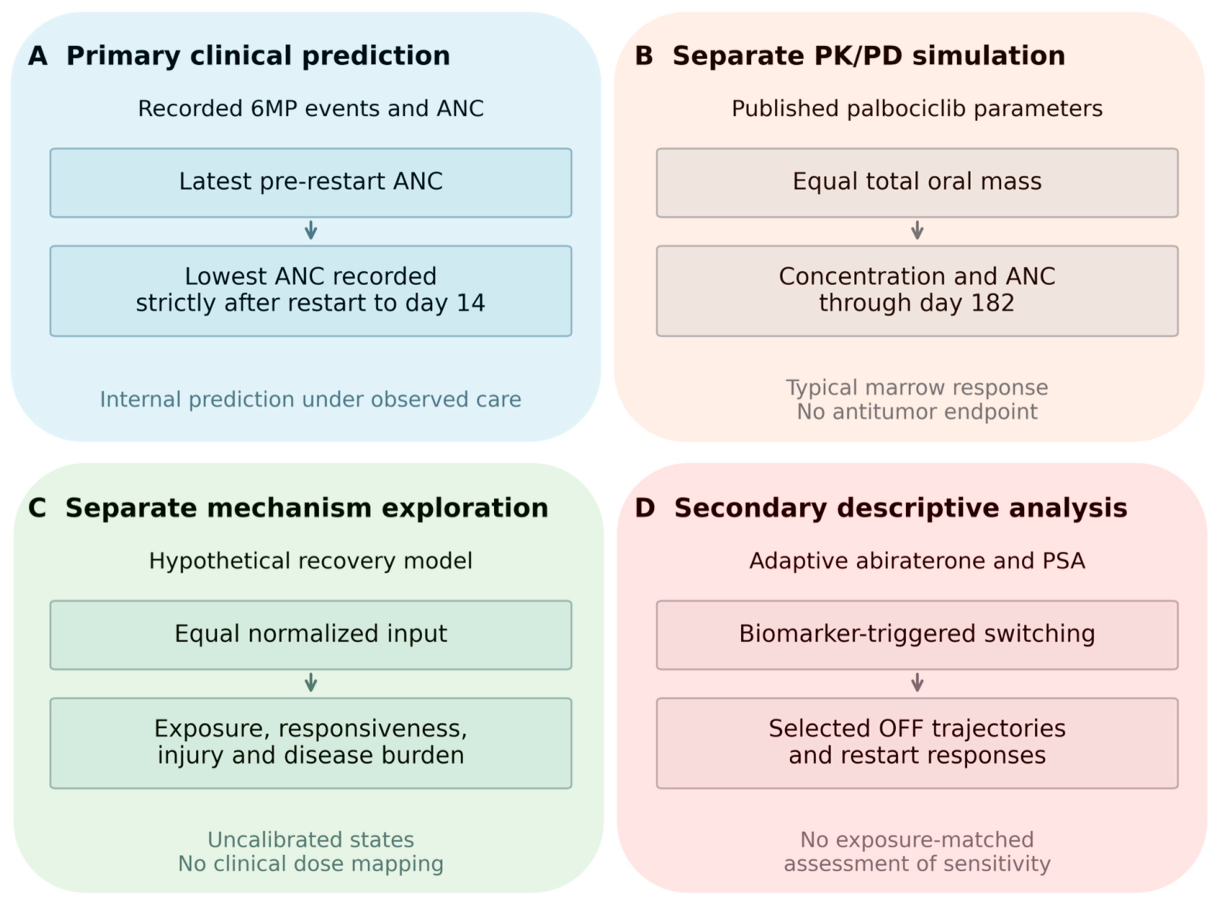
Figure 2.
Recorded 6MP episode eligibility and observation. A: selection from 55,305 event rows to 132 episodes in 73 patients, with a separate 113-episode analysis requiring at least two follow-up visits. B: missing anchors and outcomes. Candidate gaps require consecutive dose records >1.50 days apart, and eligible gap duration is ≥2.99 days. Outcomes are the lowest ANC recorded strictly after restart through day 14. Counts are episodes/unique patients unless stated otherwise. No 14-day outcome windows overlap within a patient (the recorded gaps do not establish treatment withholding).
Figure 2.
Recorded 6MP episode eligibility and observation. A: selection from 55,305 event rows to 132 episodes in 73 patients, with a separate 113-episode analysis requiring at least two follow-up visits. B: missing anchors and outcomes. Candidate gaps require consecutive dose records >1.50 days apart, and eligible gap duration is ≥2.99 days. Outcomes are the lowest ANC recorded strictly after restart through day 14. Counts are episodes/unique patients unless stated otherwise. No 14-day outcome windows overlap within a patient (the recorded gaps do not establish treatment withholding).
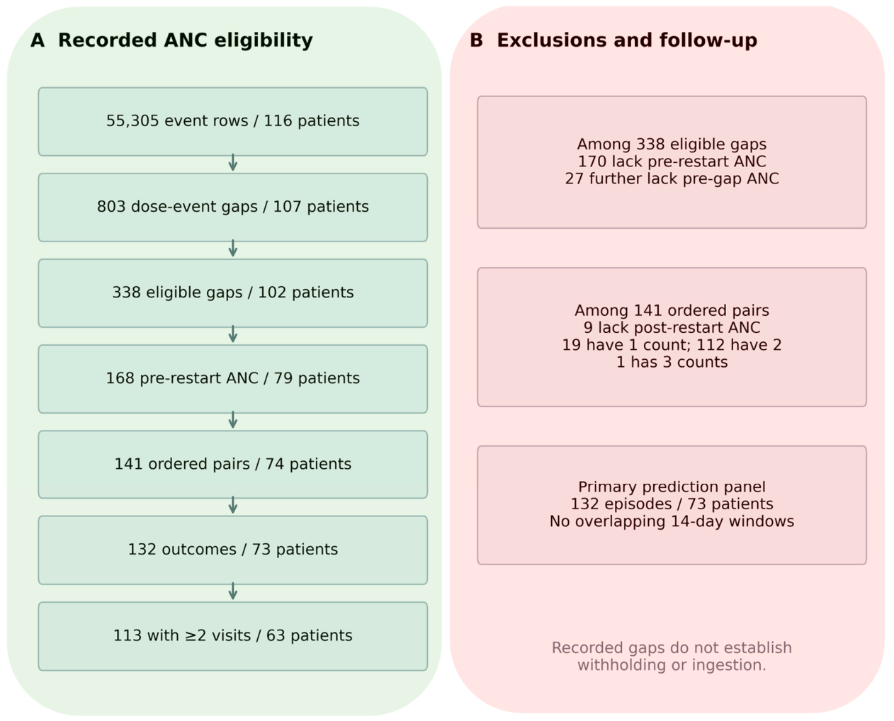
Figure 3.
Predictive association and internal ANC prediction. A: pre-restart ANC and the minimum recorded in (0,14] days for 132 episodes in 73 patients. The inset displays 0–4 G/L while the full range remains visible. The scatter is unadjusted and noncausal. B: patient-weighted LOPO RMSE with separate fitting for the ≥2-visit panel. C: paired MSE reductions in (G/L)² and patient-cluster bootstrap 95% percentile intervals from 2,000 full-retraining draws. These are MSE-reduction intervals, not RMSE intervals (the ≥2-visit interval includes zero).
Figure 3.
Predictive association and internal ANC prediction. A: pre-restart ANC and the minimum recorded in (0,14] days for 132 episodes in 73 patients. The inset displays 0–4 G/L while the full range remains visible. The scatter is unadjusted and noncausal. B: patient-weighted LOPO RMSE with separate fitting for the ≥2-visit panel. C: paired MSE reductions in (G/L)² and patient-cluster bootstrap 95% percentile intervals from 2,000 full-retraining draws. These are MSE-reduction intervals, not RMSE intervals (the ≥2-visit interval includes zero).
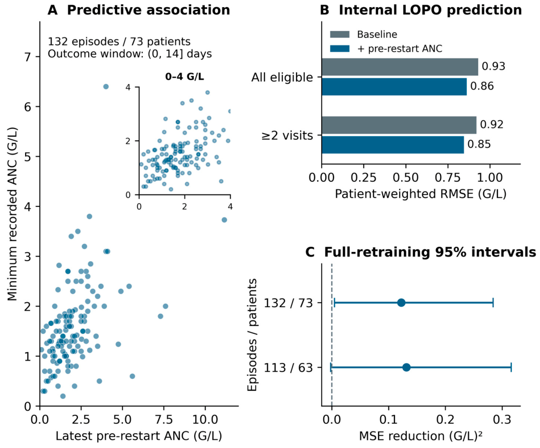
Figure 4.
Typical-parameter palbociclib simulation. A: 125 mg on 21 of every 28 days and hypothetical daily 93.75 mg both deliver 15,750 mg over 168 days. The daily schedule is a non-clinical equal-total-oral-mass comparator. B: modeled nadirs are 1.13 and 1.35 G/L. The dashed line ends dosing, follow-up continues to day 182 and does not lower either nadir. Principal clearance is 57.09 L/h and feedback exponent 0.102. This simulation has no observed patient outcomes, population risk probabilities or antitumor endpoint.
Figure 4.
Typical-parameter palbociclib simulation. A: 125 mg on 21 of every 28 days and hypothetical daily 93.75 mg both deliver 15,750 mg over 168 days. The daily schedule is a non-clinical equal-total-oral-mass comparator. B: modeled nadirs are 1.13 and 1.35 G/L. The dashed line ends dosing, follow-up continues to day 182 and does not lower either nadir. Principal clearance is 57.09 L/h and feedback exponent 0.102. This simulation has no observed patient outcomes, population risk probabilities or antitumor endpoint.
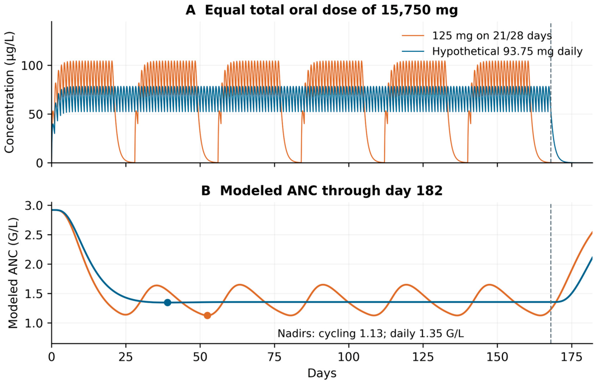
Figure 5.
Recovery and injury under specified hypothetical mechanisms. A–B: the reference periodic simulation with T≈1.68, duty 0.20, mean input one and periodic C/R/Z initialization. Shading denotes simulated administration OFF. Run identities are reported in Tables S14 and S28. C–D: finite regimens each administer 20 units from (0,1,0,1), stop input at 20 and continue to 25. The finite cycle uses period 20/12 and duty 0.20. JF is −0.02 versus 0.06. Positive values denote decreasing modeled burden. All axes are normalized and have no fitted ANC or PSA mapping.
Figure 5.
Recovery and injury under specified hypothetical mechanisms. A–B: the reference periodic simulation with T≈1.68, duty 0.20, mean input one and periodic C/R/Z initialization. Shading denotes simulated administration OFF. Run identities are reported in Tables S14 and S28. C–D: finite regimens each administer 20 units from (0,1,0,1), stop input at 20 and continue to 25. The finite cycle uses period 20/12 and duty 0.20. JF is −0.02 versus 0.06. Positive values denote decreasing modeled burden. All axes are normalized and have no fitted ANC or PSA mapping.
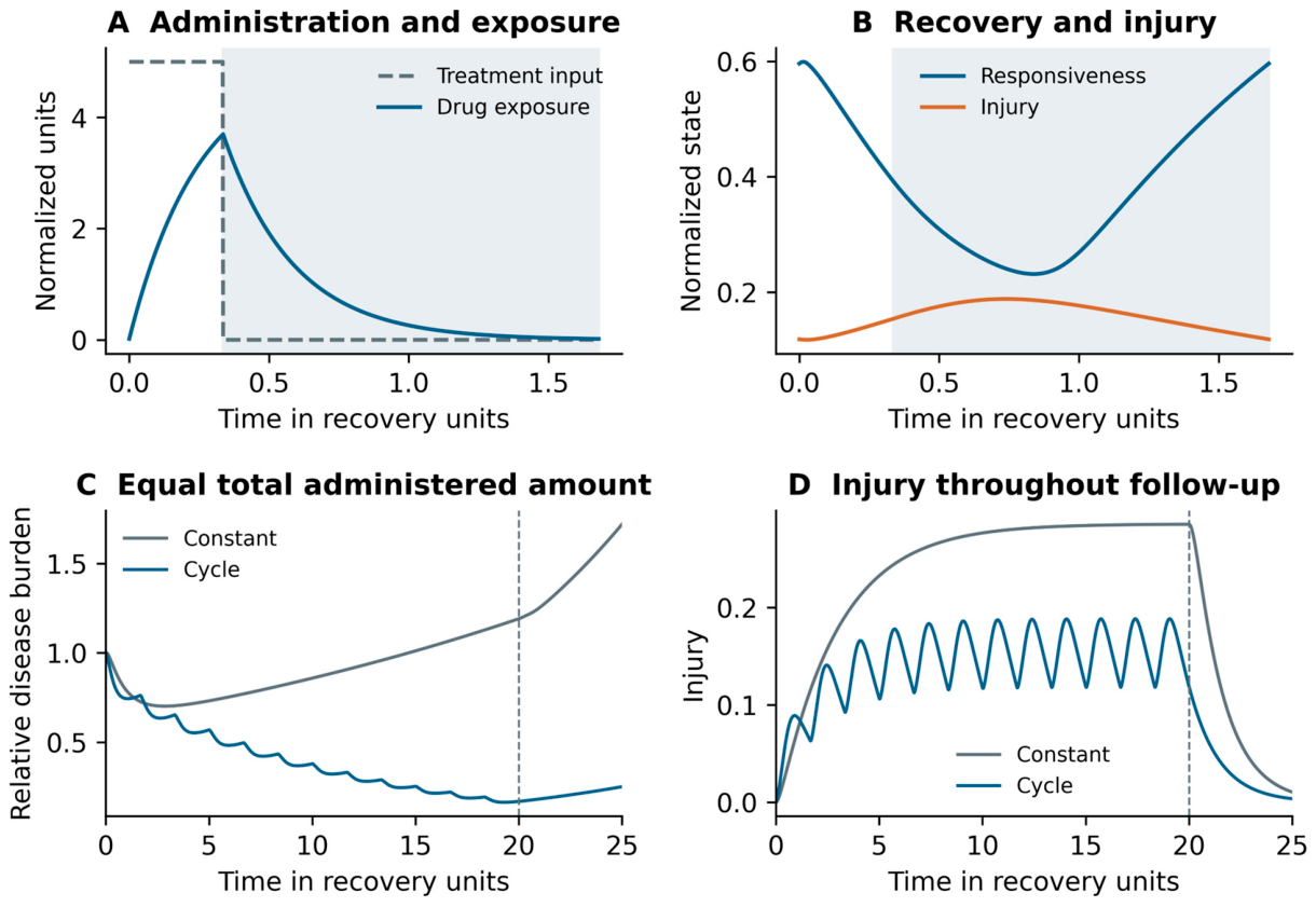
Table 1.
Clinical data and simulation components used in the assessment of treatment restart.
| Module and quantity | Measurement status | Interpretation and limit |
|---|---|---|
| ALL ANC | Measured | Recorded dose-event gaps and measured ANC. No confirmation of drug ingestion or intentional withholding. |
| Abiraterone PSA | Measured | PSA response under biomarker-triggered treatment, drug exposure unavailable. |
| Palbociclib concentration and ANC | Simulated | Typical drug exposure and delayed marrow response, no cancer-control endpoint. |
| Mechanistic exposure C | Hypothetical state | Relative exposure. Not fitted to patient drug concentrations. |
| Mechanistic responsiveness R | Hypothetical state | Recoverable treatment effect, not measured by ANC or PSA. |
| Mechanistic injury Z and burden D | Hypothetical states | Model injury and burden, not clinical ANC or PSA outcomes. |
Table 2.
Patient-weighted internal prediction and paired MSE reduction.
| Prediction sample | Baseline → enhanced RMSE | Baseline → enhanced MAE | MSE reduction and 95% interval |
|---|---|---|---|
| All outcomes 132 / 73 |
0.93 → 0.86 | 0.63 → 0.57 | 0.12 0.0047 to 0.28 |
| ≥2 visits 113 / 63 |
0.92 → 0.85 | 0.60 → 0.54 | 0.13 −0.0020 to 0.32 |
| No-dose sensitivity 132 / 73 |
0.92 → 0.85 | 0.63 → 0.57 | 0.12 0.0035 to 0.27 |
Table 3.
Typical-parameter palbociclib ANC with equal total oral mass and follow-up.
| Palbociclib model endpoint | 125 mg on 21/28 days | 93.75 mg daily |
|---|---|---|
| Total oral dose | 15,750 mg | 15,750 mg |
| ANC nadir through day 182 | 1.13 G/L | 1.35 G/L |
| Time of nadir | 52.46 days | 39.06 days |
| Final-table parameter sensitivity | 1.14 G/L | 1.36 G/L |
Table 4.
Disease control and injury in the hypothetical reference model.
| Comparison or outcome | Continuous administration | Cycling |
|---|---|---|
| Repeated cycles at equal average input | 1 model unit per time unit | 1 model unit per time unit |
| Disease-control rate during repeated cycles | −0.03 (burden increases) | 0.08 (burden decreases) |
| Peak injury during repeated cycles | 0.29 | 0.19 |
| Total administered amount over the finite course | 20 model units | 20 model units |
| Disease-control rate over the finite course | −0.02 | 0.06 |
| Burden at end of follow-up relative to baseline | 1.72 | 0.25 |
| Peak injury across the finite course | 0.29 | 0.19 |
Disclaimer/Publisher’s Note: The statements, opinions and data contained in all publications are solely those of the individual author(s) and contributor(s) and not of MDPI and/or the editor(s). MDPI and/or the editor(s) disclaim responsibility for any injury to people or property resulting from any ideas, methods, instructions or products referred to in the content. |
© 2026 by the authors. Licensee MDPI, Basel, Switzerland. This article is an open access article distributed under the terms and conditions of the Creative Commons Attribution (CC BY) license (http://creativecommons.org/licenses/by/4.0/).
Copyright: This open access article is published under a Creative Commons CC BY 4.0 license, which permit the free download, distribution, and reuse, provided that the author and preprint are cited in any reuse.