
Submitted:
11 November 2026
Posted:
12 November 2026
You are already at the latest version
Abstract
This study evaluates a forecast-informed, anomaly-aware model predictive con-trol (MPC) framework for flexible-load scheduling in a proposed ASKUE/KEGOC-oriented decision-support architecture. A univariate long short-term memory (LSTM) network generated 24-hour forecasts from 48-hour load histories, while a time-coupled optimizer enforced energy, power, and ramp-rate constraints. The evaluation used 4,380 measured-labelled hourly observations, with 648 held-out hours for scheduling. At the one-hour horizon, LSTM achieved RMSE = 0.224 kW, MAPE = 2.32%, and R² = 0.988. Under assumed flexible-load parameters, LSTM-MPC reduced the global peak by 13.21%, compared with 13.54% for seasonal-naive MPC, indicating no demonstrated scheduling advantage from LSTM forecasting. A matched AE-off/AE-on experiment then introduced identical measurement anomalies across five independently trained LSTM models. Autoencoder-triggered measurement repair using an independently retrained causal model increased mean global peak reduction from 8.70% to 12.89%. The mean paired improvement in 24-hour peak reduction was 1.077 percentage points (95% circular moving-block bootstrap interval: 0.436–1.946). All simulated schedules preserved energy and met modeled constraints. These findings support the feasibility of anomaly-aware scheduling in offline simulation, without es-tablishing physical closed-loop stability or operational deployment readiness.
Keywords:
smart grid
; model predictive control
; LSTM
; load forecasting
; flexible-load scheduling
; demand response
; autoencoder
; anomaly detection
; measurement repair
1. Introduction
The digital transformation of the electric power sector has significantly changed the principles of monitoring, forecasting, and automated control of energy consumption. Modern power systems are increasingly moving from conventional metering and centralized control toward intelligent, data-driven infrastructures capable of real-time monitoring, predictive analytics, and adaptive decision support. This transition is closely associated with the development of smart grids, advanced metering infrastructure, digital energy platforms, and artificial intelligence methods for processing large-scale energy data [1,2,3].
Smart grid technologies enable two-way communication between consumers, grid operators, distributed energy resources, and control centers. In this context, automated commercial electricity metering systems and smart meters play a key role in collecting, transmitting, and storing electricity consumption data. However, traditional metering systems are mainly focused on measurement, registration, and data transmission, while their analytical, predictive, and control capabilities remain limited [4,5]. As the number of smart meters, sensors, and connected devices increases, power systems generate large volumes of nonlinear and non-stationary time-series data that require advanced computational methods for load forecasting, anomaly detection, and optimal energy management [6,7].
Accurate electricity load forecasting is one of the most important tasks in intelligent energy systems. It supports operational planning, grid balancing, demand response, and peak load reduction. Classical statistical methods, such as ARIMA and exponential smoothing, have been widely used for time-series forecasting; however, their performance can be limited when applied to complex load profiles influenced by weather conditions, seasonality, consumer behavior, and operational constraints [8]. Machine learning and deep learning approaches provide more flexible tools for modeling nonlinear dependencies in energy consumption data. In particular, Long Short-Term Memory networks have demonstrated strong performance in short-term load forecasting because of their ability to capture long-term temporal dependencies in sequential data [9,10,11].
In addition to forecasting, intelligent energy management requires optimization mechanisms that can transform predicted load information into practical control actions. Model Predictive Control is a promising approach for automated energy management because it uses predicted system behavior over a defined horizon to calculate optimal control decisions under operational constraints [12]. In smart grid environments, MPC can support load shifting, peak shaving, cost-aware scheduling, and constrained controllable-load scheduling under operational limits. At the same time, anomaly detection is essential for identifying abnormal consumption patterns, technical faults, and possible non-technical losses. Autoencoder-based models are widely used for such tasks because they can learn normal system behavior and detect deviations through reconstruction error analysis [13].
Despite significant progress in artificial intelligence for smart grids, many existing studies consider load forecasting, optimal control, and anomaly detection as separate tasks. This limits the practical applicability of such approaches in real energy management environments, where forecasting, control, and monitoring should operate as part of a unified automated decision-support system. Moreover, limited attention has been paid to the adaptation of integrated AI-driven architectures to existing automated metering infrastructures and transmission-level power system environments.
To address this gap, this study proposes an integrated AI-based automated energy consumption management system designed for smart grid infrastructure and adapted to ASKUE/KEGOC-type energy monitoring systems. The proposed architecture combines smart meters, communication infrastructure, data preprocessing, LSTM-based load forecasting, MPC-based controllable-load scheduling, and auxiliary autoencoder-based anomaly monitoring.
The research question addressed in this study is whether a short-term data-driven load forecast provides a measurable improvement in constrained flexible-load scheduling, relative to a transparent seasonal-naive forecasting baseline. We therefore distinguish forecasting accuracy from downstream scheduling benefit and evaluate both on the same held-out hourly observations.
The main contributions of this study are: (i) the development of a time-coupled receding-horizon scheduling model incorporating flexible-load constraints and an explicit remaining-energy state; (ii) a comparative evaluation of LSTM-assisted, seasonal-naive, and perfect-information scheduling under identical simulated flexibility assumptions; (iii) a matched AE-off versus AE-on experiment examining the contribution of autoencoder-triggered causal measurement repair to downstream MPC scheduling; and (iv) an uncertainty analysis based on five independently trained LSTM models and a circular moving-block bootstrap. The proposed framework is evaluated exclusively through offline simulation. No claim of physical control authority, power-flow feasibility, or closed-loop stability is made.
2. Literature Review
2.1. Smart Grid and Advanced Metering Infrastructure
The concept of the smart grid has become one of the central directions in the modernization of electric power systems. Unlike traditional power grids, smart grids integrate digital communication, automated monitoring, intelligent control, and real-time data exchange between different participants of the energy system [1,2]. Early studies emphasized that the smart grid enables improved reliability, observability, and flexibility of power systems by combining power engineering with information and communication technologies [1,14].
Advanced Metering Infrastructure represents one of the key components of smart grid development. AMI enables the collection of high-resolution consumption data from smart meters and supports bidirectional communication between consumers and utilities [4,5]. Smart meter data can be used not only for billing purposes but also for forecasting, demand response, fault detection, and consumer behavior analysis. Alahakoon and Yu [6] highlighted that smart electricity meter data provide a foundation for future intelligent energy systems by enabling data-driven decision-making and predictive analytics. However, the effective use of AMI data requires scalable computational methods capable of processing large, heterogeneous, and time-dependent datasets.
Demand response is another important function enabled by smart metering and smart grid infrastructure [15,16]. It allows consumers and grid operators to adjust electricity consumption in response to system conditions, price signals, or operational constraints. Vardakas et al. [17] reviewed demand response programs in smart grids and showed that such mechanisms can reduce peak demand and improve grid efficiency. Similarly, game-theoretic and optimization-based approaches have been proposed to support autonomous demand-side management and distributed energy consumption scheduling [18].
2.2. Load Forecasting Using Machine Learning and Deep Learning
Electricity load forecasting has been extensively studied because of its importance for planning, dispatching, and real-time energy management. Traditional statistical methods, including ARIMA and exponential smoothing, are widely used for time-series forecasting due to their interpretability and simplicity [8]. However, these methods may be insufficient for modern smart grid data, which are often nonlinear, non-stationary, and affected by multiple external factors such as temperature, humidity, seasonality, calendar effects, and consumer behavior.
Machine learning methods have been introduced to overcome these limitations. Random Forest, Gradient Boosting, Support Vector Machines, and other supervised learning algorithms have shown good performance in energy forecasting tasks, especially when dealing with noisy and multidimensional datasets [19,20]. Random Forest models are particularly useful because they are robust to outliers, can handle nonlinear relationships, and are less sensitive to overfitting compared with individual decision trees [19].
Deep learning methods have further improved the ability to model complex temporal patterns in electricity consumption [9]. Long Short-Term Memory networks are especially suitable for load forecasting because they are designed to learn dependencies in sequential data over long time intervals [10]. Kong et al. [11] demonstrated the effectiveness of LSTM recurrent neural networks for short-term residential load forecasting. Marino et al. [21] also showed that deep neural networks can be successfully applied to building energy load forecasting. These studies confirm the relevance of deep learning models for energy consumption prediction; however, in many cases, forecasting is considered separately from downstream control and anomaly detection tasks.
Justification for Selecting LSTM over Advanced Recurrent Architectures
Recent studies show that recurrent neural networks remain widely used for short-term load and power forecasting because they can model nonlinear temporal dependencies in sequential energy data. Conventional LSTM networks are effective for one-step-ahead and short-horizon forecasting tasks because they process historical load observations in chronological order and preserve information through memory cells and gating mechanisms. This property is important for practical smart grid applications, where only past and current measurements are available for real-time forecasting and decision support.
More advanced architectures, such as BiLSTM, GRU, CNN-LSTM, and CNN-BiLSTM-Attention models, have also demonstrated strong forecasting performance. BiLSTM can process sequences in both forward and backward directions and may improve accuracy when the complete input sequence is available during offline training. For example, the recommended study on deep learning forecasting models in Energies discusses LSTM, GRU, BiLSTM, and BiGRU architectures and their role in energy-related time-series forecasting. However, BiLSTM may introduce additional computational complexity and is less directly aligned with strictly causal online forecasting, where future observations are not available at the prediction time. Recent studies also show that hybrid CNN-BiLSTM-Attention models can improve forecasting accuracy by combining feature extraction, bidirectional temporal modeling, and attention mechanisms, but such models require larger datasets and more extensive hyperparameter tuning.
Therefore, a conventional LSTM architecture was selected in this study for three reasons. First, the main objective of the paper is not to propose a new forecasting architecture, but to use the forecast as predictive input for MPC-based controllable-load scheduling. Second, LSTM provides a good balance between forecasting accuracy, interpretability, computational complexity, and compatibility with real-time smart metering workflows. Third, the available dataset is described in aggregated and anonymized form, and the use of a more complex BiLSTM or hybrid CNN-BiLSTM-Attention model would require a broader multi-season dataset and a more extensive architecture-selection study. Nevertheless, the comparison with BiLSTM, GRU, CNN-LSTM, and attention-based hybrid models is recognized as an important direction for future work.
2.3. Model Predictive Control in Energy Management
Model Predictive Control is widely used in automation and control systems because it can optimize system behavior over a future prediction horizon while considering constraints [12]. In energy systems, MPC is useful because it can use forecasted load values to generate control actions aimed at minimizing deviations from target consumption levels, reducing operational costs, and smoothing peak demand.
The main advantage of MPC is its ability to repeatedly update control decisions as new measurements become available. This makes it suitable for dynamic and uncertain environments such as smart grids, where electricity demand, generation, weather conditions, and operational constraints can change over time. MPC has been applied in energy management systems, microgrids, building automation, and demand response applications. However, the effectiveness of MPC depends strongly on the quality of input forecasts. Therefore, the integration of MPC with accurate AI-based forecasting models, such as LSTM, can improve the performance of intelligent energy management systems.
2.4. Anomaly Detection in Smart Metering Systems
Anomaly detection is an important task in smart grid and AMI environments. Abnormal consumption patterns may indicate technical faults, metering errors, cyber-physical irregularities, or non-technical losses. Traditional rule-based methods are often insufficient for detecting complex and hidden anomalies in high-dimensional time-series data. Therefore, machine learning and deep learning approaches have been increasingly used for anomaly detection in energy systems.
Nizar et al. [22] investigated non-technical loss analysis using machine learning methods and showed that data-driven models can improve the identification of irregular consumption behavior. Autoencoders are also effective for anomaly detection because they can learn compact representations of normal data and detect deviations through reconstruction error [13]. Sakurada and Yairi [13] demonstrated the use of autoencoders for nonlinear dimensionality reduction and anomaly detection. In smart metering systems, this approach is particularly useful because it does not always require large labeled anomaly datasets, which are often difficult to obtain in real power system environments.
2.5. Research Gap
The literature shows that LSTM models are effective for short-term load forecasting, while MPC is widely used for constrained predictive control in energy systems [11,12]. However, many studies use forecasting models only for prediction accuracy assessment and do not explicitly show how forecasted demand is transformed into controllable-load scheduling decisions. In addition, MPC-based energy management studies often assume the availability of a predictive model but do not sufficiently discuss the effect of forecasting errors, controllable-load limits, or anomaly-related data reliability on the scheduling process.
The autoencoder is further evaluated through a matched scheduling ablation in which its anomaly flags trigger a predefined measurement-repair policy, allowing the downstream effect of anomaly-aware input processing to be assessed under controlled simulation conditions.
Therefore, the research gap addressed in this study is the development of an LSTM-assisted MPC framework in which the LSTM forecast is used as the future demand trajectory for constrained controllable-load scheduling. The autoencoder module is not considered as an independent primary contribution; instead, it is used as an auxiliary anomaly monitoring component that helps identify abnormal conditions under which MPC recommendations should be interpreted with caution.

Table 1.
Comparative analysis of related studies and the proposed framework.
| Study direction | Typical methods | Main focus | Limitation | Difference of proposed study |
| Classical load forecasting | ARIMA, exponential smoothing | Short-term prediction | Limited ability to model nonlinear load behavior | Uses LSTM for nonlinear temporal dependencies |
| Machine learning forecasting | Random Forest, SVM, Gradient Boosting | Forecasting accuracy | Usually not connected to control actions | Connects forecasting output to MPC-based controllable-load scheduling |
| Deep learning forecasting | LSTM, DNN, CNN-LSTM | Load prediction | Often evaluated as isolated forecasting task | Integrates LSTM with MPC and anomaly detection |
| MPC-based energy management | MPC, optimization algorithms | Peak shaving, load shifting | Depends on forecasting accuracy | Uses LSTM forecast as predictive input |
| Anomaly detection | Autoencoder, clustering, classification | Fault or abnormal behavior detection | Often separated from energy management decisions | Uses anomalies for operational decision support |
| Proposed framework | LSTM-assisted MPC + auxiliary autoencoder monitoring | Controllable-load scheduling based on load forecasts | Requires pilot validation and formal robust MPC analysis | Uses LSTM forecast as the predictive demand trajectory for MPC-based controllable-load scheduling; autoencoder supports anomaly-aware monitoring |
3. Materials and Methods
3.1. General Research Design
This study proposes an integrated AI-based automated energy consumption management system intended for smart grid and automated commercial electricity metering infrastructure. The methodological basis of the research combines energy consumption data acquisition, preprocessing, short-term load forecasting, predictive control, and anomaly detection within a unified automated workflow. The proposed approach is designed for ASKUE/KEGOC-type infrastructure, where electricity consumption data are collected from smart metering devices and transmitted to a data processing and decision-support layer. The development of such digital energy management tools is also relevant to national priorities for modernization and digital transformation of the electric power sector in Kazakhstan [23].
The research methodology consists of the following main stages: data collection from smart metering and monitoring sources, preprocessing and normalization of hourly load time series, development of an LSTM forecasting model, transformation of LSTM forecasts into predictive demand trajectories, formulation of an MPC-based controllable-load scheduling problem, evaluation of scheduling performance using peak load and load-balancing indicators, and auxiliary anomaly monitoring using an autoencoder. The LSTM-assisted MPC module constitutes the main methodological component of the proposed framework, while the autoencoder provides anomaly monitoring and measurement-quality information for the evaluated anomaly-aware scheduling procedure [1,4,5,11,12,13].
3.2. Proposed System Architecture
The proposed system is organized as a multi-level automated architecture that supports the complete cycle of energy consumption management, from measurement to decision-making [24,25,26,27,28]. The architecture includes five main layers:
Measurement layer, consisting of smart meters and IoT-based measuring devices that collect electricity consumption parameters, including active power, voltage, current, and total energy consumption.
The proposed communication architecture is conceptually aligned with the interoperability principles discussed in the IEC 61850 series, which addresses communication networks and information exchange in power utility automation systems [24]. The specific communication interfaces were not implemented or validated in the present offline simulation.
Data processing layer, which performs storage, aggregation, cleaning, filtering, and normalization of incoming time-series data.
Intelligent analytical layer, where the main LSTM-assisted MPC workflow is implemented. First, the LSTM module generates a short-term forecast of future electricity demand. Second, the MPC module uses this forecast as the predictive demand trajectory for controllable-load scheduling under operational constraints. In parallel, the autoencoder module monitors reconstruction errors and generates anomaly flags when abnormal input conditions are detected [27].
Decision-support and control layer, which generates recommendations and control actions for load redistribution, peak shaving, demand response, and anomaly response.
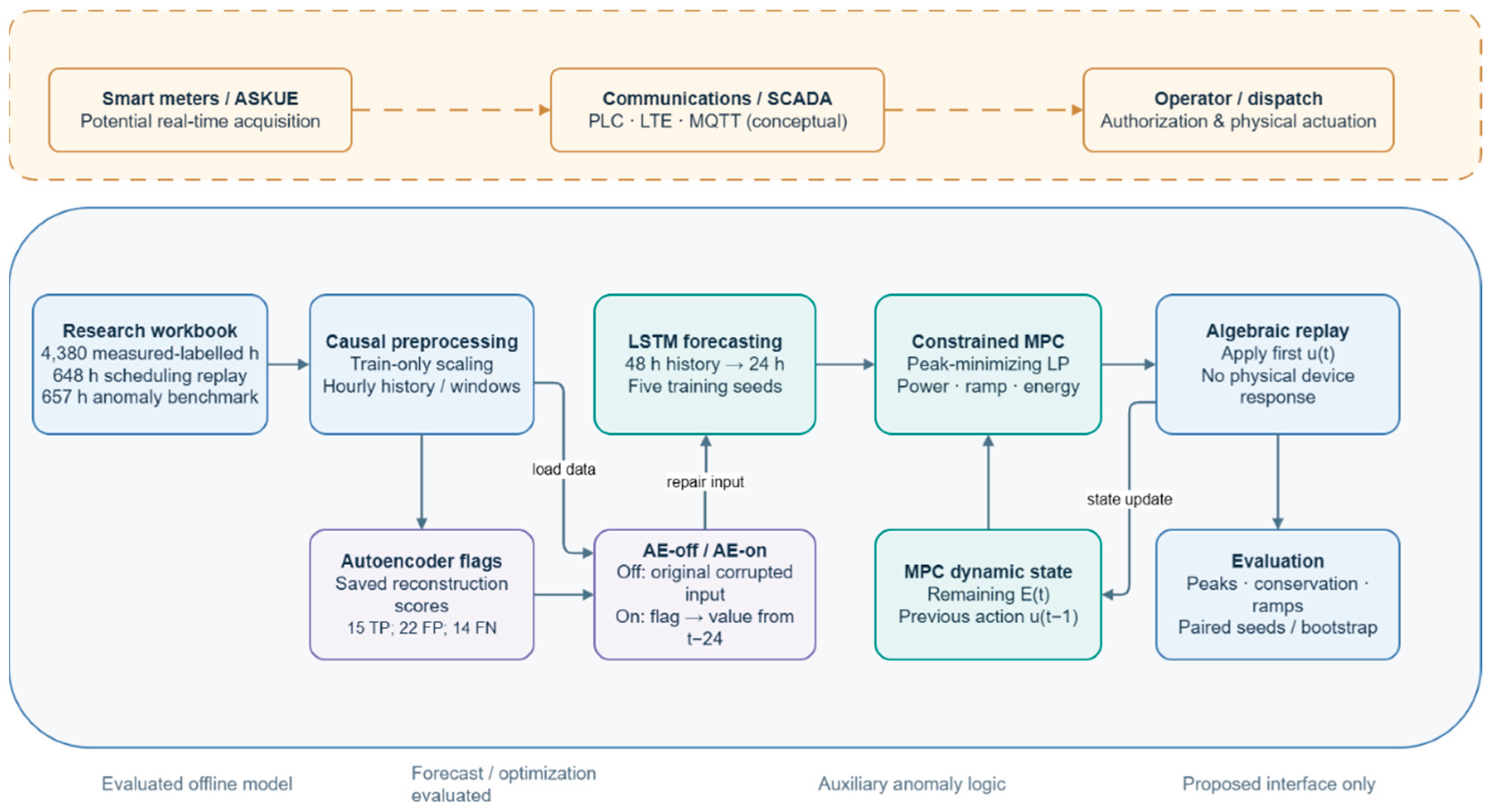
The proposed architecture consists of a measured-load input layer, data-quality and forecasting modules, a constrained scheduling optimizer and a decision-support output. The present evaluation is an offline replay simulation: historical observations are sequentially revealed to the forecast model, the optimizer computes a proposed flexible-load setpoint, and the resulting aggregate demand is obtained from an algebraic load-shifting model. The physical response of individual devices and the operator’s dispatch system are not simulated. The feedback shown in the conceptual architecture therefore denotes the update of the software optimization problem, not demonstrated feedback control of an electrical power network.
Figure 1.
Conceptual decision-support architecture for offline replay of LSTM-informed flexible-load scheduling. Dashed links to dispatch and metering infrastructure indicate proposed integration, not an implemented field interface.
Figure 1.
Conceptual decision-support architecture for offline replay of LSTM-informed flexible-load scheduling. Dashed links to dispatch and metering infrastructure indicate proposed integration, not an implemented field interface.
3.3. Data Description and Input Variables
The study used an author-compiled research dataset derived from electricity-consumption information originating from KEGOC JSC. The analytical workbook comprises 4,380 hourly measurement-derived observations covering the period from 25 July 2025 to 23 January 2026. The dataset was preprocessed and chronologically divided into training, validation, and testing subsets. An additional 4,380-hour synthetic extension was excluded from the primary experimental evaluation. All experiments were performed offline without direct access to operational dispatch or control systems.
The dataset includes active- and reactive-power variables and was prepared for computational analysis through preprocessing and chronological partitioning. The measured-labelled component was divided into 3,066 training observations, 657 validation observations, and 657 test observations.
An additional 4,380-hour synthetic extension was generated separately to complete the annual research dataset. This synthetic component was excluded from the primary forecasting, anomaly-detection, and MPC scheduling experiments.
The research workbook represents an author-prepared analytical dataset based on company information rather than a directly validated export from KEGOC's operational control systems. The experiments were conducted exclusively through offline simulation, without direct interaction with operational dispatch or control infrastructure.
The tested forecasting configuration is univariate and uses historical aggregate active power (kW) only. Although the input workbook may contain auxiliary variables, the present LSTM experiment does not establish an effect of weather or calendar covariates.
Table 2.
Composition and chronological allocation of the author-compiled research dataset.
| Dataset component | Observations | Use / status |
|---|---|---|
| Measured-labelled hourly series | 4,380 | Training 3,066 / validation 657 / test 657 |
| Measured test used for scheduling | 648 | 27 consecutive 24-hour blocks |
| Synthetic extension | 4,380 | Excluded from primary experiment |
| Sampling interval | 1 h | Active power in kW |
Controllable Load Model
At test hour t, observed aggregate demand Pₜ is decomposed in the simulation into an uncontrollable component bₜ = Pₜ − F and a nominal flexible component F. The scheduled aggregate load is Pₜˢ = bₜ + uₜ = Pₜ − F + uₜ, where uₜ denotes the scheduled flexible power. The nominal flexible power was set to F = 1.9265 kW, corresponding to 20% of the training-set mean power. This is a synthetic flexibility assumption, not an inventory of controllable KEGOC assets.
Flexible demand satisfies 0 ≤ uₜ ≤ 3.8529 kW. Across consecutive hours, including the boundary between scheduling blocks, |uₜ − uₜ₋₁| ≤ 1.5412 kW. For each 24-hour block W, the energy service is constrained by Σₜ∈W uₜΔt = 46.2353 kWh, with Δt = 1 h. The remaining service-energy state evolves according to Eₜ₊₁ = Eₜ − uₜΔt, with E initialized to 46.2353 kWh at the start of each 24-hour block. This couples decisions over time, preserves the block energy of the original profile, and prevents unrestricted peak shaving by curtailment. The assumed base and flexible components are not independently measured.
3.4. Data Preprocessing
Only the measured-labelled active-power series was used as input. Scaling parameters were computed exclusively from the 3,066 training observations: zₜ = (Pₜ − μtrain)/σtrain. The same training parameters were used for validation and testing, and predictions were transformed back to kW before evaluation and scheduling. The network received the preceding 48 hourly load values and predicted the following 24 values. All windows were assigned chronologically; training and validation target windows were restricted to their respective partitions, while forecasting at test times used only observations available at the corresponding decision instant. No future test targets were included in the network input at prediction time.
3.5. LSTM-Based Load Forecasting Model
The forecasting model was implemented in PyTorch as a univariate LSTM with a 48-hour lookback and direct 24-hour output. The recurrent layer contains 24 hidden units; its final hidden output is passed through a 48-unit ReLU dense layer and a 24-unit linear output layer. The mean-squared-error objective was optimized with Adam at a learning rate of 0.002, using batches of approximately 128 windows and a maximum of 50 epochs. The checkpoint was selected on validation loss with an early-stopping patience of nine epochs, using a minimum improvement threshold of 0.0002 in normalized MSE. Random seeds were fixed at 42 for NumPy and PyTorch in the recorded run.
For each test decision hour t, the model generated forecasts (P̂ₜ|ₜ, …, P̂ₜ₊₂₃|ₜ) using only the previous 48 measured values. A seasonal-naive comparator predicted the load at each horizon step from the corresponding observed hour in the preceding 24-hour cycle. This design permits direct comparison of forecasting errors and the resulting schedules under identical optimization settings.
Table 3.
Actual hyperparameters of the reproduced forecasting run.
| Hyperparameter | Implemented value |
| Input sequence | 48 hourly loads |
| Output horizon | 24 hourly loads, direct multi-output |
| LSTM hidden units | 24 |
| Dense head | 48 ReLU → 24 linear |
| Additional input features | None (univariate load only) |
| Optimizer / learning rate | Adam / 0.002 |
| Loss / batch size | MSE / approximately 128 |
| Maximum epochs / early stopping | 50 / patience 9 |
| Seed | 42 |
| Model selection | Lowest validation loss, min improvement 0.0002 |
3.6. LSTM-Assisted MPC for Controllable Load Scheduling
A receding-horizon linear program was solved at each test hour t over the remaining Hₜ = 24 − ((t − t₀) mod 24) hours of the current scheduling block. Define decision vector uₜ,…,uₜ₊Hₜ₋₁, auxiliary variable z for forecast peak power, and nonnegative deviation variables dₖ. The implemented objective is:
subject to
dₖ ≥ uₜ+ₖ − F;
dₖ ≥ F − uₜ+ₖ;
0 ≤ uₜ+ₖ ≤ 2F;
|uₜ+ₖ − uₜ+ₖ−1| ≤ 0.8F
(using the previously applied action at k = 0);
Eₜ₊₁ = Eₜ − uₜΔt.
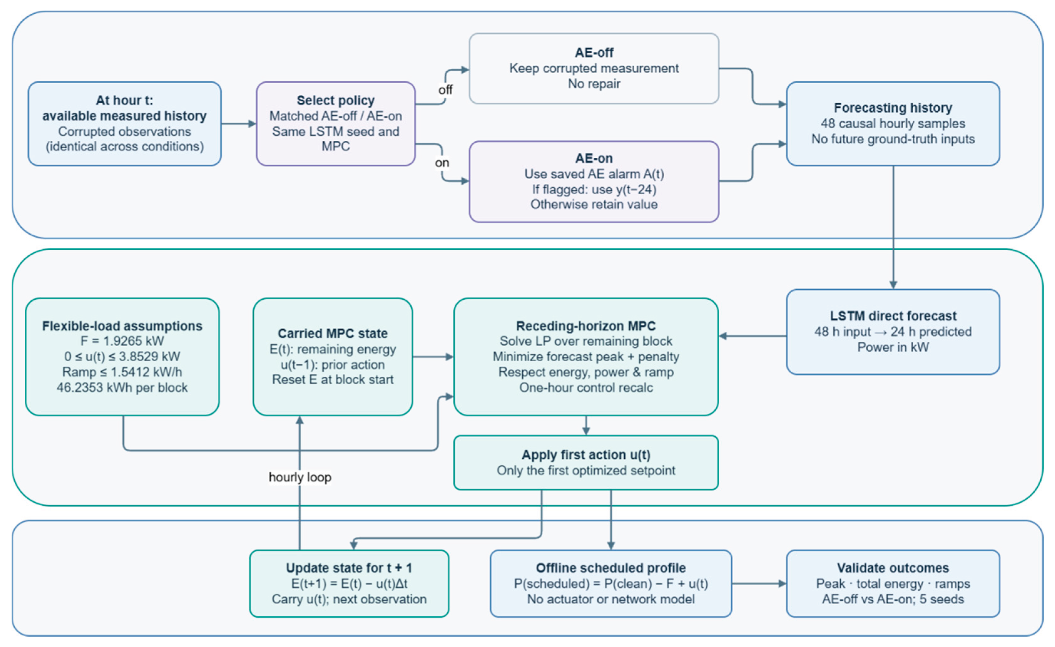
Only the first optimized flexible-load value is applied in the simulation; after one hour, the next available observation is incorporated and the problem is resolved. The previous applied control action is transferred across adjacent 24-hour blocks, so the ramp bound remains active over the entire 648-hour axis. The service-energy state resets to 24FΔt only at a block boundary, because each block represents a new independent flexible-energy requirement. In this model, applying a schedule means algebraically adding the scheduled flexible load to the inferred base load; it does not simulate equipment response dynamics.
The controllable-load model was parameterized according to the magnitude of the evaluated test profile. A nominal flexible demand of 1.9265 kW, a maximum controllable power of 3.8529 kW, and an hourly ramp bound of 1.5412 kW were assumed for the simulation. These values describe a hypothetical flexible-load portfolio and are not derived from documented equipment ratings or transmission-network operating limits.
Figure 2.
Chronological offline replay of 24-hour direct load forecasting, state-coupled receding-horizon scheduling, first-action simulation and measurement update. This is an algorithmic feedback loop, not validated physical closed-loop control.
Figure 2.
Chronological offline replay of 24-hour direct load forecasting, state-coupled receding-horizon scheduling, first-action simulation and measurement update. This is an algorithmic feedback loop, not validated physical closed-loop control.
3.6.1. Forecast-Horizon Diagnostics and Scheduling Baselines
Forecast evaluation was conducted using aligned target–prediction pairs from the same held-out test interval. The one-step metrics are reported over 648 test hours, and horizon-specific errors are calculated only for forecast steps with observed targets available inside the same 648-hour test segment. Forecasting quality is evaluated independently of the downstream peak-shaving objective. Three scheduling strategies share the same controllable-power, ramp and energy constraints: seasonal-naive MPC, LSTM-assisted MPC and an oracle MPC supplied with actual future demand. The oracle is an unattainable perfect-information benchmark rather than an implementable controller. No claim is made that LSTM forecasts improve scheduling unless the paired scheduling results support such an improvement.
Table 4.
Horizon-specific forecasting errors from aligned measured test targets.
| Forecast horizon | LSTM RMSE (kW) | Seasonal RMSE (kW) | LSTM MAPE (%) | Seasonal MAPE (%) |
| 1 h | 0.224 | 0.664 | 2.32 | 6.20 |
| 6 h | 0.375 | 0.666 | 3.90 | 6.22 |
| 12 h | 0.552 | 0.667 | 5.54 | 6.22 |
| 24 h | 0.653 | 0.667 | 6.38 | 6.18 |
3.6.2. Conservative Constraint Handling Under Forecast Uncertainty
The implemented controller is a receding-horizon optimization algorithm evaluated in an offline algebraic replay. It enforces modeled capacity, ramp and energy-service constraints on the computed flexible-load setpoints and preserves the continuity of the previously applied setpoint across block boundaries. Constraint satisfaction was verified numerically on the 648-hour simulated schedules. The reported zero violations refer only to these modeled constraints, not to voltage, frequency, transmission-line, thermal or actuator constraints.
The experiment does not include a state-space model of physical network dynamics, identification of device response, bounded process disturbances, a terminal invariant set, a terminal cost, a stability certificate or a proof of recursive feasibility for arbitrary disturbances. Accordingly, an iterative software feedback arrow must not be interpreted as evidence of stable physical closed-loop control. The results support the feasibility of the tested scheduling problem under its assumptions; operational closed-loop validation remains future work.
3.6.3. Matched Anomaly-Aware MPC Ablation Study
To evaluate the contribution of anomaly-aware input processing to downstream scheduling performance, a matched AE-off versus AE-on experiment was conducted using the same held-out electricity load series, identical anomaly injections, and identical MPC optimization constraints.
The evaluation covered 648 consecutive hourly observations, corresponding to 27 successive 24-hour scheduling blocks. Within this interval, 29 controlled measurement anomalies were introduced. The independently retrained causal autoencoder correctly detected 15 anomalous observations and generated 22 false-positive alerts. The remaining 14 injected anomalies were not detected. These fixed anomaly flags were used to evaluate the downstream effect of the predefined measurement-repair policy in the matched AE-off versus AE-on MPC experiment.
Controlled measurement anomalies were introduced into the active-power observation channel using four perturbation levels: −100%, −65%, +30%, and +65% relative to the corresponding uncorrupted measurement. Reactive-power observations were retained as the second autoencoder input feature without injected modifications. The supplied validation scenario contained 36 anomalous observations among 657 hourly records, whereas the independent test scenario contained 30 anomalous observations among 657 records. The first 648 test records, used for matched MPC replay, contained 29 injected anomalies. The anomaly positions and corrupted measurements were preserved in the supplied research dataset, enabling exact replay of the evaluated scenarios. The original randomization procedure used to select these positions was not independently recovered.
Five independently trained LSTM models were considered, with random seeds 42, 7, 21, 123, and 2026. Each model used a 48-hour input sequence, a direct 24-hour forecasting horizon, and the same forecasting architecture. The two experimental conditions were evaluated using the same pretrained model for each corresponding seed.
In the AE-off condition, corrupted observations entered the forecasting history without correction. In the AE-on condition, an observation flagged by the autoencoder was replaced by the previously available observation corresponding to the same hour 24 hours earlier. Previously repaired observations were retained in the input history, and no future target values or anomaly ground-truth labels were used to determine the replacement.
Both configurations employed the same receding-horizon linear optimization model, objective function, energy requirement, flexible-power limits, and ramp-rate constraints. The first optimized control action was applied at each simulation step, while the previous action and remaining energy requirement were maintained as required by the scheduling model.
Injected anomalies affected only the measurement channel. The simulated scheduled load was evaluated against the original, uncorrupted demand series. The comparison therefore isolates the effect of the specified anomaly-triggered measurement-repair policy within the offline scheduling simulation.
Performance was assessed using global peak demand, average 24-hour peak reduction, one-hour forecasting RMSE, energy conservation, power-bound violations, ramp-rate violations, and optimization feasibility.
3.7. Auxiliary Autoencoder-Based Anomaly Monitoring
The autoencoder was employed as a measurement-quality monitoring module within the proposed anomaly-aware scheduling framework. It reconstructed two-dimensional input vectors containing Min–Max normalized active- and reactive-power measurements. The model was trained using normal operating observations, and reconstruction errors were compared with a threshold selected on the validation set.
During offline evaluation, each newly available observation was processed independently to generate an anomaly flag without accessing future measurements. In the AE-on configuration, flagged active-power measurements triggered a predefined replacement procedure using the corresponding observation from 24 hours earlier. The resulting measurement history was supplied to the LSTM forecasting model, while the MPC optimization constraints remained unchanged. No physical dispatch actions were implemented.
Table 5.
Autoencoder architecture and anomaly detection settings.
| Component | Description |
|---|---|
| Input features | Active power and reactive power |
| Input dimension | 2 |
| Data preprocessing | Min–Max scaling |
| Encoder layers | 64 → 32 → 16 |
| Decoder layers | 32 → 64 → 2 |
| Hidden activation | ReLU |
| Output activation | Sigmoid |
| Reconstruction loss | Mean squared error |
| Optimizer | Adam |
| Learning rate | 0.001 |
| Batch size | 32 |
| Maximum epochs | 100 |
| Early stopping | Patience = 10 |
| Random seed | 42 |
| Selected validation percentile | 99 |
| Anomaly threshold | 0.0002564189617987695 |
The encoder transformed the two-dimensional normalized active- and reactive-power input vector into a 16-dimensional learned latent representation through successive fully connected layers, while the decoder reconstructed the original two input features. Reconstruction errors were calculated in the normalized feature space and compared with the validation-selected threshold.
Min–Max normalization parameters were estimated exclusively from the first 3,066 training observations. The subsequent 657 validation observations were used for early stopping and threshold selection. Model training was limited to 100 epochs with an early-stopping patience of 10 epochs. The best checkpoint was obtained at epoch 70, and training terminated at epoch 80.
The detection threshold was selected from the 90th, 95th, 97.5th, and 99th percentiles of clean validation reconstruction errors. The percentile yielding the highest F1-score on controlled validation anomalies was retained. The selected threshold corresponded to the 99th percentile, yielding a normalized reconstruction-error threshold of 0.000256419. Because injected anomaly labels were used to select the percentile, threshold selection constitutes supervised validation tuning rather than a fully unsupervised selection procedure.
The trained autoencoder, normalization parameters, and threshold were fixed before evaluation on the independent 657-observation test set. Each reconstruction score was computed from the currently available active- and reactive-power measurement only, without accessing subsequent observations or test labels. A numerical causality check confirmed that modifications to future observations did not alter previously generated reconstruction scores.
In the evaluated offline scheduling ablation, autoencoder anomaly flags were used to trigger a predefined measurement-repair policy. Flagged observations were replaced by the previously available value corresponding to the same hour of the preceding day, and the resulting corrected measurement history was supplied to the LSTM forecaster. The procedure was assessed through matched AE-off and AE-on simulations under identical injected anomalies. MPC constraints remained unchanged, and no physical dispatch commands were issued.
The reconstruction error is calculated as (8):
where x is the original input vector, is the reconstructed output vector generated by the autoencoder, and E(x) is the reconstruction error.
The anomaly decision rule is defined as (9):
where A(x)=1 indicates an anomaly, A(x)=0 indicates normal behavior, and θ is the anomaly detection threshold.
In addition to its independent anomaly-classification evaluation, the autoencoder was incorporated into a matched offline scheduling ablation. Its output was used exclusively as a binary measurement-quality indicator that triggered a predefined causal input-repair procedure. When an observation was flagged as anomalous, the corresponding load measurement was replaced by an available seasonal reference value from 24 hours earlier before being used in subsequent LSTM forecasts.
The autoencoder did not directly modify physical equipment commands, change MPC optimization constraints, or guarantee the correctness of the repaired observation. The AE-on and AE-off configurations were compared under identical controlled anomaly injections to evaluate whether this monitoring-assisted repair mechanism affected simulated scheduling performance.
For anomaly-aware scheduling, detection scores must be available at the corresponding decision time. The monitoring procedure therefore requires a strictly causal reconstruction window containing only current and previously observed measurements. The anomaly decision must be completed before the affected observation is admitted to the LSTM forecasting history. This timing requirement is essential to prevent future-information leakage in the offline replay. The independently retrained autoencoder computes each reconstruction score from the current two-dimensional observation using fixed training-derived normalization parameters, thereby preventing future-observation leakage in the evaluated offline implementation.
The observed scheduling benefit is conditional on the selected anomaly types, detector operating threshold, replacement policy, and simulation assumptions. No physical closed-loop stability or safety guarantee is inferred from the anomaly-monitoring results.
3.8. Evaluation Metrics
The performance of the proposed system was evaluated using forecasting, control, and anomaly detection metrics.
The forecasting accuracy metrics MAPE, RMSE, and R² were used to quantify the difference between actual and predicted load values. MAPE expresses the average relative forecasting error in percentage form, RMSE measures the magnitude of prediction errors in the same physical unit as the target variable, namely kW, and R² evaluates how well the predicted load values explain the variability of the actual load profile. These metrics are widely used in time-series forecasting and load forecasting studies [34].
For anomaly monitoring, accuracy, precision, recall, and F1-score were used to evaluate the classification performance of the autoencoder-based anomaly flag. Accuracy measures the overall proportion of correctly classified observations, precision evaluates the proportion of correctly detected anomalies among all predicted anomalies, recall measures the ability of the model to identify actual anomalies, and F1-score provides a harmonic mean of precision and recall. These metrics are commonly used for binary classification and anomaly detection evaluation [35].
For load forecasting, Mean Absolute Percentage Error (MAPE) (10), Root Mean Square Error (RMSE) (11), and coefficient of determination R² (12) were used:
Root Mean Square Error (RMSE) was used instead of MSE because it is expressed in the same unit as the target variable, namely kW (11).
where Pi is the actual load, is the predicted load, is the mean actual load over the evaluation sample, and n is the number of observations.
For anomaly detection, accuracy, precision, recall, and F1-score were used (13), (14), (15):
The F1-score was calculated as the harmonic mean of precision and recall (16):
where TP, TN, FP, and FN represent true positives, true negatives, false positives, and false negatives.
All forecast metrics are calculated on identical time-aligned pairs (yᵢ, ŷᵢ), with RMSE = sqrt[(1/n)Σᵢ(yᵢ−ŷᵢ)²], MAPE = (100/n)Σᵢ|yᵢ−ŷᵢ|/|yᵢ| and R² = 1−Σᵢ(yᵢ−ŷᵢ)²/Σᵢ(yᵢ−ȳ)². The evaluated loads are strictly positive. For each scenario, the global peak reduction is 100×(max P − max Pˢ)/max P, whereas the mean period-level reduction is the arithmetic mean of 27 separate 24-hour peak reductions. These are different estimands and must not be conflated.
To characterize descriptive uncertainty, 10,000 percentile-bootstrap resamples of the 27 scheduling blocks were generated with replacement for the mean period-level peak reduction and the paired LSTM-minus-seasonal difference. These intervals do not adjust for dependence between neighboring blocks and should not be interpreted as a formal generalization guarantee. For autoencoder binary metrics, 95% Wilson binomial intervals were computed descriptively.
For the matched anomaly-aware MPC experiment, an additional dependence-aware uncertainty analysis was conducted. The LSTM forecasting model was independently trained using five random seeds (42, 7, 21, 123, and 2026), and the same trained model was used in each matched AE-off and AE-on comparison.
The primary paired effect was defined as the difference between AE-on and AE-off in the percentage reduction of the maximum load within each 24-hour scheduling block. This measure was evaluated using the same uncontrolled peak as the reference for both configurations.
To account for temporal dependence between adjacent scheduling blocks, a circular moving-block bootstrap was implemented using blocks of four consecutive 24-hour periods. A total of 20,000 bootstrap replicates were generated, with additional resampling of the five model seeds.
The resulting percentile-based 95% confidence interval was used to describe uncertainty in the mean paired improvement. These estimates reflect the selected test interval, injected anomaly protocol, and model initializations; they do not constitute a formal guarantee of performance under different operating conditions.
The LSTM was implemented in PyTorch, and the scheduling optimization used SciPy linear programming with the HiGHS solver. Both the observation split and the scheduled trajectories are time ordered. The uncontaminated reference forecasting experiment used random seed 42. The matched anomaly-aware MPC ablation employed five independently trained LSTM models with seeds 42, 7, 21, 123, and 2026.
3.9. Implementation Tools and Reproducibility
The experiments were implemented in Python. The LSTM forecasting models were developed and trained using PyTorch, while constrained receding-horizon scheduling was performed using SciPy linear programming with the HiGHS optimization solver. NumPy was used for numerical operations, data processing, and statistical analysis.
The reconstruction-error scores and binary anomaly flags used in the matched AE-off versus AE-on MPC experiment were generated using the independently retrained autoencoder. The model employed training-derived normalization parameters and a fixed validation-selected detection threshold. The resulting test-set reconstruction scores and anomaly flags were preserved and subsequently used in the offline scheduling comparison. This procedure ensures that the reported ablation results are associated with the newly retrained model rather than the unavailable original autoencoder implementation.
Five independent LSTM training runs were performed with fixed random seeds to evaluate sensitivity to model initialization. A circular moving-block bootstrap was applied to characterize uncertainty in the paired scheduling outcomes.
The anomaly-detection module was independently retrained in PyTorch using the supplied measured-labelled active- and reactive-power data. The complete training implementation, trained model weights, training-derived normalization parameters, validation threshold-selection results, and reconstruction scores for all 657 held-out observations were preserved. The accompanying scripts reproduce the anomaly classification results and the matched AE-off versus AE-on MPC experiment.
The newly retrained model represents an independently reproducible implementation rather than an exact recovery of the original autoencoder, whose trained weights and implementation were unavailable. Temporal causality was verified for the new model, whose reconstruction scores depend only on current observations and fixed parameters estimated before the test interval.
The study was conducted entirely in offline simulation. No live SCADA interface, physical smart-meter communication channel, or operational KEGOC control infrastructure was implemented or experimentally validated. These components remain part of the proposed conceptual architecture.
4. Results
4.1. Load Forecasting Performance
On the 648-hour measured test subset used in the scheduling replay, the direct multi-output LSTM achieved a one-hour-ahead RMSE of 0.224 kW, MAPE of 2.32% and R² of 0.988. The seasonal-naive predictor yielded 0.664 kW, 6.20% and 0.895, respectively. Every metric in Table 6 was computed on the same test targets, and therefore the three error indicators are mutually consistent. The LSTM forecast was substantially more accurate at the one-hour horizon, but the gain narrowed at the longer prediction horizons. This forecasting comparison must be distinguished from the downstream scheduling comparison.
4.2. Comparison of Actual and Predicted Load
The comparison between actual and predicted electricity consumption values showed that the LSTM model closely followed the real load profile. The predicted curve reproduced the main characteristics of electricity demand, including daily fluctuations, short-term changes, and peak consumption intervals.
Figure 3 compares the measured-labelled test demand with one-hour-ahead LSTM and seasonal-naive forecasts over 96 consecutive test hours. The LSTM generally follows the observed profile more closely at this horizon, as reflected by the RMSE and MAPE results in Table 6. However, this forecasting advantage did not translate into a demonstrated improvement in global peak reduction compared with seasonal-naive MPC.
As illustrated in Figure 3, the LSTM predictor follows the observed daily load pattern more closely than the seasonal-naive benchmark over the displayed 96-hour interval. The quantitative evaluation across the 648-hour test segment confirms the lower one-hour forecasting error of the LSTM model, as reported in Table 6.
However, forecasting accuracy and downstream scheduling effectiveness represent different evaluation objectives. Although the LSTM provides more accurate short-term predictions, the comparison of scheduling strategies does not establish a corresponding improvement in peak reduction relative to the seasonal-naive MPC baseline.
4.3. Results of LSTM-Assisted MPC-Based Controllable Load Scheduling
The corrected MPC evaluation uses 648 consecutive held-out measured observations partitioned into 27 adjacent 24-hour scheduling blocks. For all compared optimizers, the initial nominal flexible demand is F = 1.9265 kW, its permitted range is [0, 3.8529] kW, the hourly ramp limit is 1.5412 kW, and the required energy per block is 46.2353 kWh. The previous applied action is carried over across block boundaries. The simulated LSTM-assisted schedule reduced the global maximum from 11.818 to 10.257 kW, a 13.21% reduction. Seasonal-naive scheduling yielded 10.218 kW, or 13.54%, and the perfect-information oracle reached 9.892 kW, or 16.30%. All calculated trajectories conserved the 5,410.97 kWh aggregate energy of the observed test segment and satisfied the stated flexible-power, ramp and energy-service constraints.
Because the seasonal benchmark achieved a slightly lower global test peak than the LSTM-informed controller, the present experiment does not establish superior downstream scheduling from LSTM forecasting. These values are outcomes of a simulated flexible-load portfolio rather than measured reductions at a KEGOC facility.
Figure 4 illustrates the uncontrolled and simulated scheduled active-power trajectories over the first 96 hours of the held-out test interval. The scheduled trajectories were obtained using the algebraic flexible-load model and do not represent measured physical control actions at a KEGOC installation. The corresponding global peak-load reductions and constraint-verification results are summarized in Table 7.
As shown in Figure 4, the MPC control trajectory follows the general trend of the actual load while smoothing fluctuations and supporting a more balanced load profile. The LSTM forecast provides the predictive input for the control process, while the MPC module generates a regulated load trajectory under predefined operating constraints. These results indicate the potential of the proposed framework for predictive load management and peak reduction. These visual results are consistent with the quantitative indicators presented in Table 7, where peak load, load factor, and constraint violations improved after LSTM-assisted MPC-based controllable-load scheduling.
Across the 27 consecutive 24-hour blocks, the mean peak reduction was 14.48% for LSTM-assisted MPC (95% percentile-bootstrap interval: 13.82–15.06%) and 14.37% for seasonal-naive MPC (13.66–15.04%). The paired mean difference (LSTM minus seasonal) was 0.109 percentage points (95% interval: −0.486 to 0.690 percentage points). The interval includes zero. Consequently, the present data provide no statistically conclusive evidence of a scheduling advantage attributable to the LSTM predictor. These block-based intervals are descriptive and do not correct for serial dependence or training-seed variability; they must not be confused with uncertainty intervals for the global maximum reduction.
The Model Predictive Control algorithm was evaluated in terms of its ability to reduce peak load, improve the load factor, and avoid constraint violations.
4.4. Auxiliary Anomaly Monitoring Results
The independently retrained autoencoder was evaluated using 657 held-out observations, including 30 controlled injected anomalies and 627 normal observations. The model correctly detected 16 anomalies, generated 22 false-positive alerts, and missed 14 anomalies, while 605 normal observations were correctly classified.
The resulting classification performance was 94.52% accuracy, 42.11% precision, 53.33% recall, and 47.06% F1-score. The 95% Wilson confidence intervals were 36.14–69.77% for recall and 27.85–57.81% for precision.
Compared with the previously preserved autoencoder outputs, the independently retrained model achieved higher recall but lower precision and F1-score. This trade-off indicates that improved detection sensitivity was accompanied by an increased number of false-positive alarms.
Figure 5 presents the reconstruction-error scores of all 657 held-out observations, together with the fixed validation-selected threshold of 0.000256419. The figure distinguishes correctly detected anomalies, missed anomalies, and false-positive detections.
For the subsequent matched MPC experiment, the first 648 held-out observations were used. This interval contained 29 injected anomalies, of which 15 were detected. The autoencoder generated 37 alarms, comprising 15 true-positive and 22 false-positive detections, while 14 injected anomalies remained undetected.
For context, the Isolation Forest baseline achieved 8 true positives, 23 false positives, 22 false negatives and 604 true negatives on the supplied comparison, corresponding to 93.15% accuracy, 25.81% precision, 26.67% recall and 26.23% F1. These results describe the independent anomaly-detection benchmark. The autoencoder flags were subsequently used in a separate matched AE-on versus AE-off scheduling experiment. The downstream scheduling results are presented in Section 4.5. The results are presented in Table 8.
Table 8.
Performance of the autoencoder-based anomaly detection model.
| Detector | Accuracy (%) | Precision (%) | Recall (%) | F1-score (%) |
|---|---|---|---|---|
| Retrained Autoencoder | 94.52 | 42.11 | 53.33 | 47.06 |
| Isolation Forest (previous benchmark) | 93.15 | 25.81 | 26.67 | 26.23 |
Table 9.
Autoencoder confusion matrix (n = 657).
| Actual condition | Predicted normal | Predicted anomaly |
|---|---|---|
| Normal | 605 (TN) | 22 (FP) |
| Injected anomaly | 14 (FN) | 16 (TP) |
4.5. Matched AE-Off Versus AE-on MPC Results
The matched AE-off versus AE-on MPC experiment was repeated using anomaly flags generated by the independently retrained causal autoencoder. Both configurations were evaluated under identical injected measurement anomalies, LSTM model initializations, optimization objectives, and scheduling constraints.
Within the 648-hour simulation interval, the retrained autoencoder detected 15 of the 29 injected anomalies and produced 22 false-positive alerts. In the AE-on configuration, flagged measurements were replaced using previously available observations from the corresponding hour 24 hours earlier. The AE-off configuration retained the corrupted measurements without correction.
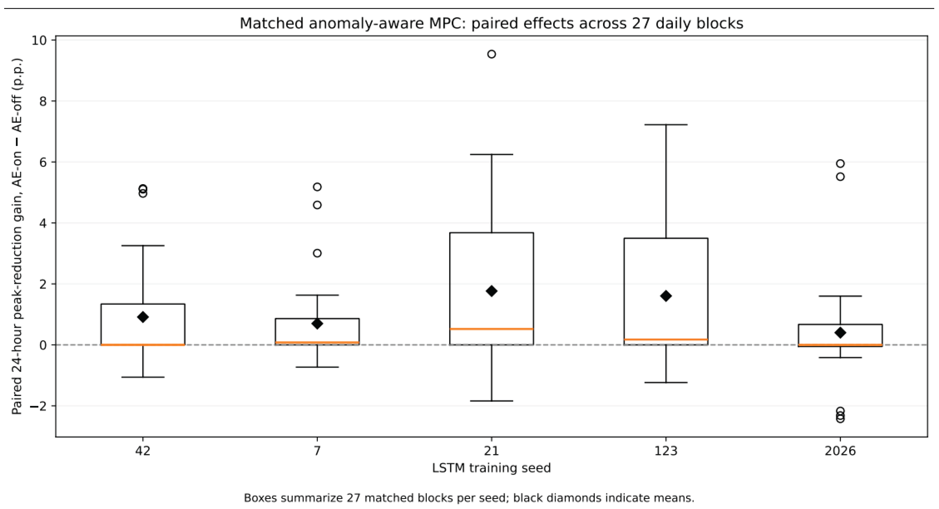
Across five independently trained LSTM models, mean global peak reduction was 8.70% for AE-off and 12.89% for AE-on. The mean paired improvement in 24-hour peak-load reduction was 1.077 percentage points, with a descriptive 95% circular moving-block bootstrap confidence interval of 0.436–1.946 percentage points.
Mean one-hour forecasting RMSE decreased from 0.737 kW in the AE-off configuration to 0.481 kW in the AE-on configuration. All ten evaluated MPC schedules preserved the total energy of 5,410.968 kWh and satisfied the assumed controllable-power, ramp-rate, and 24-hour energy-service constraints without optimization failures.
These findings indicate that the independently retrained causal autoencoder, combined with the specified measurement-repair policy, improved simulated scheduling performance under controlled measurement anomalies. Nevertheless, the experiment does not establish physical closed-loop stability or operational reliability in an actual power system.
Table 10.
Matched AE-off and AE-on MPC scheduling results across five independently trained LSTM models.
Table 10.
Matched AE-off and AE-on MPC scheduling results across five independently trained LSTM models.
| Seed | AE-off peak (kW) | AE-on peak (kW) | AE-off reduction (%) | AE-on reduction (%) |
|---|---|---|---|---|
| 42 | 10.698 | 10.507 | 9.48 | 11.09 |
| 7 | 10.971 | 10.359 | 7.17 | 12.35 |
| 21 | 10.767 | 10.266 | 8.89 | 13.13 |
| 123 | 10.638 | 10.168 | 9.98 | 13.96 |
| 2026 | 10.874 | 10.171 | 7.99 | 13.94 |
| Mean | 10.790 | 10.294 | 8.70 | 12.89 |
Note: Global peak reductions were calculated separately for each model seed. The mean paired improvement in 24-hour peak-reduction percentage (1.077 percentage points) represents a different statistical measure.
Figure 6.
Comparison of global peak-load reductions obtained with AE-off and AE-on MPC across five independently trained LSTM models under identical injected measurement anomalies.
Figure 6.
Comparison of global peak-load reductions obtained with AE-off and AE-on MPC across five independently trained LSTM models under identical injected measurement anomalies.
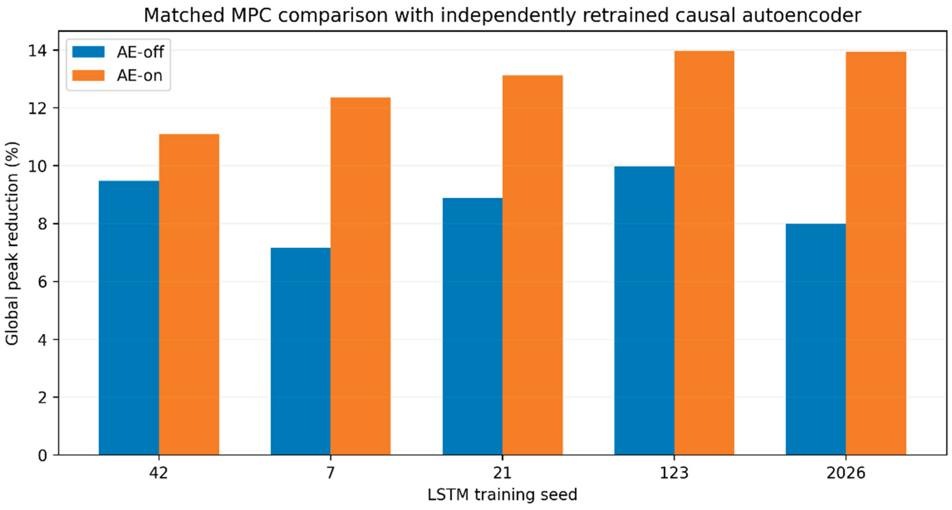
Across the five model initializations, AE-off MPC produced a mean global peak of 10.790 kW, corresponding to a mean peak reduction of 8.70% relative to the uncontrolled reference peak of 11.818 kW. With autoencoder-triggered measurement repair enabled, the mean global peak decreased to 10.294 kW, corresponding to a mean global peak reduction of 12.89%.
Figure 7.
Paired differences in 24-hour peak-load reduction between AE-on and AE-off MPC across 27 consecutive scheduling blocks and five LSTM seeds.
Figure 7.
Paired differences in 24-hour peak-load reduction between AE-on and AE-off MPC across 27 consecutive scheduling blocks and five LSTM seeds.
All ten evaluated MPC schedules preserved the total energy of 5,410.968 kWh, satisfied the modeled controllable-power and ramp constraints, and produced no optimization infeasibilities. Energy conservation and constraint satisfaction were verified using the same uncorrupted reference demand for both configurations.
4.6. Integrated System Performance
The experimental evaluation provides evidence for three complementary functions of the proposed framework: accurate short-term load forecasting, constrained receding-horizon scheduling, and anomaly-aware measurement processing.
The uncontaminated forecasting experiment demonstrates that the LSTM model achieves lower one-hour prediction errors than the seasonal-naive benchmark. The scheduling experiment confirms that the proposed optimization model can reduce peak demand while preserving energy under the specified flexibility constraints. However, the LSTM-informed scheduling configuration does not demonstrate a statistically established advantage over seasonal-naive MPC.
The additional matched anomaly-aware ablation demonstrates that autoencoder-triggered causal measurement repair improves simulated scheduling performance relative to an AE-off baseline under the selected controlled anomaly conditions. The experiment includes independent LSTM training runs and temporally dependent bootstrap resampling to characterize uncertainty.
These findings extend the evaluation beyond independent forecasting and anomaly classification, while retaining important limitations. The framework remains an offline decision-support simulation without validated physical device dynamics, network-level operational constraints, or demonstrated closed-loop stability. The main experimental outcomes of the proposed system are summarized in Table 11.
5. Discussion
The study illustrates how a direct multi-hour load forecast can be used as an input to a temporally coupled optimization problem for simulated flexible-load scheduling. The implemented scheduling model explicitly represents remaining flexible-load energy, constrains consecutive control actions, and preserves the required energy service within each 24-hour block. Its numerical feasibility was confirmed on the held-out 648-hour evaluation interval. This represents evidence for the internal consistency of a simplified scheduling simulator, not for voltage or frequency stability of a physical grid.
The forecasting and control results reveal a distinction between predictive accuracy and operational value. LSTM forecasting markedly outperformed seasonal-naive forecasting at the one-hour horizon. However, the seasonal-naive MPC schedule achieved a slightly better global peak reduction (13.54% versus 13.21%), while the paired interval for the mean 24-hour reduction difference included zero. The prediction model should therefore be described as an evaluated component of the architecture rather than as a proven source of superior scheduling decisions. Longer-horizon errors, alternative objective weights and different flexibility portfolios may change this comparison and warrant further investigation.
The independent retraining experiment strengthens the reproducibility of the proposed anomaly-aware scheduling framework. The reconstructed autoencoder implementation enables causal anomaly detection using only currently available active- and reactive-power measurements and fixed training-derived preprocessing parameters.
The retrained model achieved 53.33% recall and 42.11% precision, indicating a trade-off between increased anomaly sensitivity and false-positive detections. Despite this limitation, the matched AE-on configuration improved simulated scheduling performance relative to AE-off under identical controlled measurement anomalies. The mean paired gain was 1.077 percentage points, with a descriptive 95% circular moving-block bootstrap interval of 0.436–1.946 percentage points.
The observed improvement should be interpreted as the combined effect of anomaly detection and the predefined causal measurement-repair strategy. Its magnitude may depend on the anomaly injection procedure, threshold selection, and assumed flexible-load characteristics. The results do not imply that all anomalous observations are reliably identified or that the framework guarantees safe physical closed-loop operation.
Several limitations must be considered. First, the dataset comprises a limited measured-labelled observation period, and its original operational provenance requires independent confirmation. Second, the assumed flexible-load capacity and ramp constraints were not derived from documented controllable equipment. Third, the experiment represents an algebraic load-shifting simulation rather than a validated physical grid-control implementation. Fourth, the dependence-aware bootstrap characterizes uncertainty within the available sample but does not establish generalization to other operating conditions.
Future research should evaluate the proposed method using verified equipment-level load models, multiple independent datasets, and realistic communication and actuation delays. Additional studies should compare anomaly detectors, investigate alternative causal measurement-repair strategies, and assess robustness under different anomaly types and forecasting errors. Physical closed-loop stability, recursive feasibility under disturbances, and network-level operational constraints must be investigated before practical deployment.
6. Conclusions
This study developed and evaluated an LSTM-assisted receding-horizon scheduling framework for flexible electricity demand, supplemented by autoencoder-based anomaly monitoring and causal measurement repair.
Using 648 held-out hourly observations, the LSTM forecasting model achieved a one-hour-ahead RMSE of 0.224 kW, MAPE of 2.32%, and R² of 0.988. Under the assumed flexibility constraints, LSTM-informed MPC reduced the global peak load by 13.21%, while seasonal-naive MPC achieved 13.54%. These findings demonstrate feasible energy-preserving scheduling but do not establish superior peak-reduction performance attributable to the LSTM predictor.
The independently retrained causal autoencoder achieved 94.52% accuracy, 42.11% precision, 53.33% recall, and 47.06% F1-score on 657 held-out observations containing controlled injected anomalies. In the matched anomaly-aware scheduling experiment, enabling autoencoder-triggered measurement repair increased mean global peak reduction from 8.70% to 12.89% across five independently trained LSTM models. The mean paired improvement in 24-hour peak reduction was 1.077 percentage points, with a descriptive 95% circular moving-block bootstrap interval of 0.436–1.946 percentage points. These results support the reproducibility and simulation-level effectiveness of the newly implemented anomaly-aware scheduling procedure, while leaving physical closed-loop stability and operational deployment unverified.
All evaluated schedules preserved total energy and satisfied the modeled power and ramp constraints. Nevertheless, the improvement is specific to the simulated anomaly conditions and measurement-repair policy. The experiment does not establish operational reliability, physical closed-loop stability, or safety guarantees for a transmission-level electricity network.
The main contribution is therefore a reproducible simulation-based evaluation of forecast-informed and anomaly-aware flexible-load scheduling within a proposed ASKUE/KEGOC-oriented architecture. Future validation requires verified operational data, physical equipment models, broader robustness testing, and controlled real-world implementation.
Author Contributions
Conceptualization, G.M. and K.A.; methodology, G.M., K.A. and M.B.; software, G.M.; validation, G.M., K.A., M.B. and S.B.; formal analysis, G.M. and M.B.; investigation, G.M., M.B. and T.K.; resources, K.A., M.M. and S.B.; data curation, G.M. and M.B.; writing—original draft preparation, G.M.; writing—review and editing, K.A., M.B., M.M., T.K. and S.B.; visualization, G.M. and M.B.; supervision, K.A. and S.B.; project administration, K.A. and S.B.; funding acquisition, K.A. and S.B. All authors have read and agreed to the published version of the manuscript.
Funding
This research received no external funding.
Data Availability Statement
The underlying electricity-consumption records and the author-compiled research dataset are not publicly deposited. Access to the underlying data and their redistribution are subject to applicable third-party data-use restrictions and authorization. Model configurations, computational methods, and derived experimental results are documented in the manuscript and associated reproducibility materials.
Conflicts of Interest
The authors declare no conflict of interest.
Abbreviations
The following abbreviations are used in this manuscript:
| AI | Artificial Intelligence |
| AMI | Advanced Metering Infrastructure |
| ASKUE | Automated System for Commercial Electricity Metering |
| ARIMA | Autoregressive Integrated Moving Average |
| DNN | Deep Neural Network |
| DR | Demand Response |
| GSM | Global System for Mobile Communications |
| IoT | Internet of Things |
| KEGOC | Kazakhstan Electricity Grid Operating Company |
| LSTM | Long Short-Term Memory |
| MAPE | Mean Absolute Percentage Error |
| MPC | Model Predictive Control |
| MQTT | Message Queuing Telemetry Transport |
| PLC | Power Line Communication |
| RMSE | Root Mean Square Error |
| SCADA | Supervisory Control and Data Acquisition |
| Smart Grid | Intelligent Electric Power Grid |
| Smart Meter | Intelligent Electricity Meter |
| R² | Coefficient of Determination |
References
- Farhangi, H. The path of the smart grid. IEEE Power Energy Mag. 2010, 8, 18–28. [Google Scholar] [CrossRef]
- International Energy Agency. Digitalization and Energy; IEA: Paris, France, 2017. [Google Scholar]
- World Economic Forum. Fostering Effective Energy Transition 2024; World Economic Forum: Geneva, Switzerland, 2024. [Google Scholar]
- KEGOC. Annual Report 2024; KEGOC: Astana, Kazakhstan, 2025. [Google Scholar]
- IEEE. IEEE Guide for Smart Grid Interoperability of Energy Technology and Information Technology Operation with the Electric Power System (EPS), End-Use Applications, and Loads; IEEE Std 2030-2011; IEEE: New York, NY, USA, 2011. [CrossRef]
- Alahakoon, D.; Yu, X. Smart Electricity Meter Data Intelligence for Future Energy Systems: A Survey. IEEE Trans. Ind. Inform. 2016, 12, 425–436. [Google Scholar] [CrossRef]
- Gubbi, J.; Buyya, R.; Marusic, S.; Palaniswami, M. Internet of Things: A vision, architectural elements, and future directions. Future Gener. Comput. Syst. 2013, 29, 1645–1660. [Google Scholar] [CrossRef]
- Box, G.E.P.; Jenkins, G.M.; Reinsel, G.C.; Ljung, G.M. Time Series Analysis: Forecasting and Control, 5th ed.; Wiley: Hoboken, NJ, USA, 2015. [Google Scholar]
- Goodfellow, I.; Bengio, Y.; Courville, A. Deep Learning; MIT Press: Cambridge, MA, USA, 2016. [Google Scholar]
- Hochreiter, S.; Schmidhuber, J. Long short-term memory. Neural Comput. 1997, 9, 1735–1780. [Google Scholar] [CrossRef] [PubMed]
- Kong, W.; Dong, Z.Y.; Jia, Y.; Hill, D.J.; Xu, Y.; Zhang, Y. Short-term residential load forecasting based on LSTM recurrent neural network. IEEE Trans. Smart Grid 2019, 10, 841–851. [Google Scholar] [CrossRef]
- Camacho, E.F.; Bordons, C. Model Predictive Control, 2nd ed.; Springer: London, UK, 2007. [Google Scholar]
- Sakurada, M.; Yairi, T. Anomaly detection using autoencoders with nonlinear dimensionality reduction. In Proceedings of the 2nd Workshop on Machine Learning for Sensory Data Analysis, MLSDA 2014, Gold Coast, Australia, 2 December 2014. [Google Scholar]
- Amin, S.M.; Wollenberg, B.F. Toward a smart grid: Power delivery for the 21st century. IEEE Power Energy Mag. 2005, 3, 34–41. [Google Scholar] [CrossRef]
- International Renewable Energy Agency. Innovation Landscape for Smart Electrification; IRENA: Abu Dhabi, United Arab Emirates, 2023. [Google Scholar]
- European Commission. Smart Grids and Energy Storage Technologies; European Commission: Brussels, Belgium, 2023. [Google Scholar]
- Vardakas, J.S.; Zorba, N.; Verikoukis, C.V. A survey on demand response programs in smart grids: Pricing methods and optimization algorithms. IEEE Commun. Surv. Tutor. 2015, 17, 152–178. [Google Scholar] [CrossRef]
- Mohsenian-Rad, A.H.; Wong, V.W.S.; Jatskevich, J.; Schober, R.; Leon-Garcia, A. Autonomous demand-side management based on game-theoretic energy consumption scheduling for the future smart grid. IEEE Trans. Smart Grid 2010, 1, 320–331. [Google Scholar] [CrossRef]
- Breiman, L. Random forests. Mach. Learn. 2001, 45, 5–32. [Google Scholar] [CrossRef]
- Géron, A. Hands-On Machine Learning with Scikit-Learn, Keras, and TensorFlow, 3rd ed.; O’Reilly Media: Sebastopol, CA, USA, 2022. [Google Scholar]
- Marino, D.L.; Amarasinghe, K.; Manic, M. Building energy load forecasting using deep neural networks. Energy Build. 2016, 135, 129–140. [Google Scholar] [CrossRef]
- Nizar, A.H.; Dong, Z.Y.; Wang, Y. Power utility nontechnical loss analysis with extreme learning machine method. IEEE Trans. Power Syst. 2008, 23, 946–955. [Google Scholar] [CrossRef]
- Ministry of Energy of the Republic of Kazakhstan. Concept for the Development of the Electric Power Industry of the Republic of Kazakhstan until 2035; Ministry of Energy of the Republic of Kazakhstan: Astana, Kazakhstan, 2024. [Google Scholar]
- International Electrotechnical Commission (IEC). Communication Networks and Systems for Power Utility Automation—Part 1-1: Introduction and Overview; IEC TR 61850-1-1:2026; IEC: Geneva, Switzerland, 2026. [Google Scholar]
- Gopstein, A.; Nguyen, C.; O'Fallon, C.; Hastings, N.; Wollman, D.A. NIST Framework and Roadmap for Smart Grid Interoperability Standards, Release 4.0; NIST Special Publication 1108r4; National Institute of Standards and Technology: Gaithersburg, MD, USA, 2021. [Google Scholar] [CrossRef]
- Institute of Electrical and Electronics Engineers (IEEE). IEEE Vision for Smart Grid Controls: 2030 and Beyond; IEEE Smart Grid Research: Control Systems; IEEE, 2013. [Google Scholar]
- Russell, S.; Norvig, P. Artificial Intelligence: A Modern Approach, 4th ed.; Pearson: Hoboken, NJ, USA, 2021. [Google Scholar]
- Alibekkyzy, K.; Belginova, S.; Batalova, M. Modeling of Quality Control Management Processes in the Development and Operation of VLC Systems. In Proceedings of the 2023 5th International Congress on Human-Computer Interaction, Optimization and Robotic Applications (HORA 2023), Istanbul, Turkey, 8–10 June 2023; IEEE: Piscataway, NJ, USA, 2023. [Google Scholar] [CrossRef]
- Tao, F.; Zhang, H.; Liu, A.; Nee, A.Y.C. Digital twin in industry: State-of-the-art. IEEE Trans. Ind. Inform. 2019, 15, 2405–2415. [Google Scholar] [CrossRef]
- International Energy Agency. Electricity Market Report 2025; IEA: Paris, France, 2025. [Google Scholar]
- Momoh, J.A. Smart Grid: Fundamentals of Design and Analysis; Wiley-IEEE Press: Hoboken, NJ, USA, 2012. [Google Scholar]
- Wang, D.; Li, S.; Fu, X. Short-Term Power Load Forecasting Based on Secondary Cleaning and CNN-BILSTM-Attention. Energies 2024, 17, 4142. [Google Scholar] [CrossRef]
- Pavlatos, C.; Makris, E.; Fotis, G.; Vita, V.; Mladenov, V. Enhancing Electrical Load Prediction Using a Bidirectional LSTM Neural Network. Electronics 2023, 12, 4652. [Google Scholar] [CrossRef]
- Hyndman, R.J.; Koehler, A.B. Another look at measures of forecast accuracy. Int. J. Forecast. 2006, 22, 679–688. [Google Scholar] [CrossRef]
- Chicco, D.; Jurman, G. The advantages of the Matthews correlation coefficient (MCC) over F1 score and accuracy in binary classification evaluation. BMC Genom. 2020, 21, 6. [Google Scholar] [CrossRef] [PubMed]
Figure 3.
Observed load, one-hour-ahead LSTM forecast and seasonal-naive forecast over the first 96 test hours; all values are in kW.
Figure 3.
Observed load, one-hour-ahead LSTM forecast and seasonal-naive forecast over the first 96 test hours; all values are in kW.
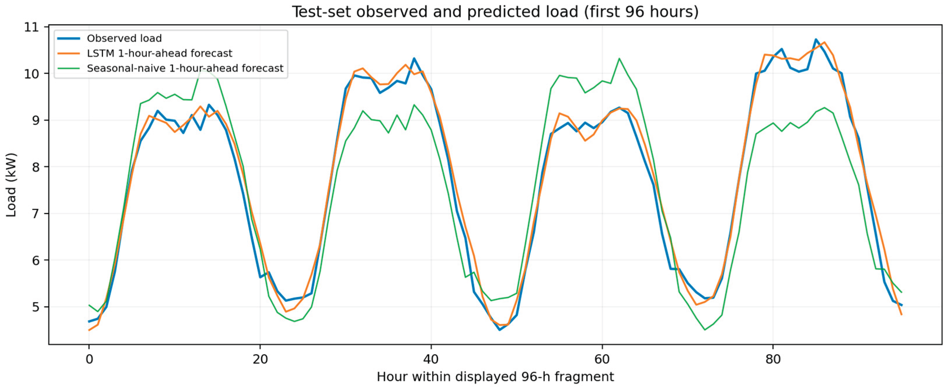
Figure 4.
Uncontrolled and simulated scheduled load profiles over the first 96 test hours. Ramp continuity is checked over all 648 hours, not only within the displayed fragment.
Figure 4.
Uncontrolled and simulated scheduled load profiles over the first 96 test hours. Ramp continuity is checked over all 648 hours, not only within the displayed fragment.
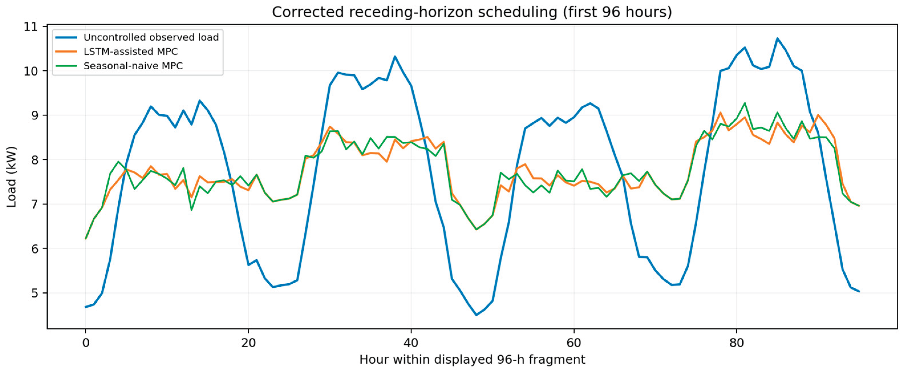
Figure 5.
Reconstruction-error scores of the independently retrained causal autoencoder across 657 held-out observations. The dashed line indicates the validation-selected threshold of 0.000256419. Detected anomalies (n = 16), missed anomalies (n = 14), and false-positive alerts (n = 22) are distinguished using separate markers. Reconstruction errors are expressed as normalized mean squared errors on a logarithmic scale.
Figure 5.
Reconstruction-error scores of the independently retrained causal autoencoder across 657 held-out observations. The dashed line indicates the validation-selected threshold of 0.000256419. Detected anomalies (n = 16), missed anomalies (n = 14), and false-positive alerts (n = 22) are distinguished using separate markers. Reconstruction errors are expressed as normalized mean squared errors on a logarithmic scale.
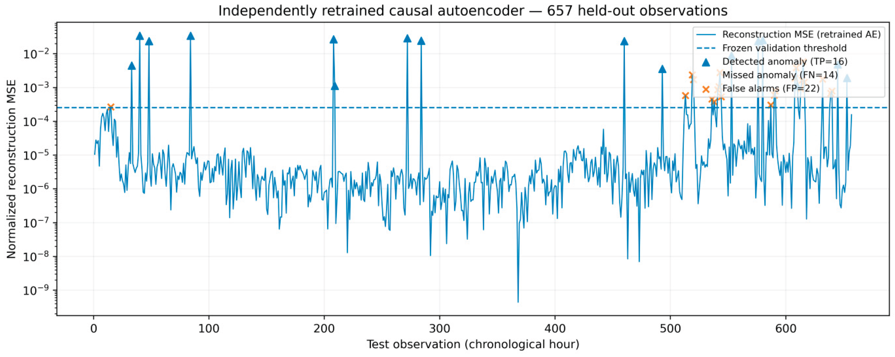
Table 6.
One-hour-ahead forecasting results on the same measured test targets.
| Forecasting method | MAPE (%) | RMSE (kW) | R² | n |
|---|---|---|---|---|
| LSTM, one-hour horizon | 2.32 | 0.224 | 0.988 | 648 |
| Seasonal-naive, one-hour horizon | 6.20 | 0.664 | 0.895 | 648 |
Table 7.
Corrected time-coupled scheduling on the 648-hour measured test segment.
| Scheduling scenario | Global peak (kW) | Peak reduction (%) | Load factor | Energy (kWh) | Modeled violations |
|---|---|---|---|---|---|
| Uncontrolled | 11.818 | — | 0.707 | 5,410.97 | — |
| Seasonal-naive MPC | 10.218 | 13.54 | 0.817 | 5,410.97 | 0 |
| LSTM-assisted MPC | 10.257 | 13.21 | 0.814 | 5,410.97 | 0 |
| Oracle MPC (unattainable) | 9.892 | 16.30 | 0.844 | 5,410.97 | 0 |
Table 11.
Supported and unsupported claims in the evaluation.
| Evidence component | Verified result | Interpretation |
|---|---|---|
| One-step forecast | LSTM RMSE 0.224 kW; naive 0.664 kW | Forecast improvement supported |
| Global test peak | LSTM 13.21%; naive 13.54% | No LSTM control gain established |
| Mean block peak reduction | LSTM 14.48%; naive 14.37% | Paired difference inconclusive |
| Anomaly detection | Recall 53.33%; precision 42.11%; F1-score 47.06% | Detection capability confirmed on injected anomalies; false alarms and missed anomalies remain |
| AE-aware MPC ablation | Mean paired gain 1.077 pp; 95% block-bootstrap CI 0.436–1.946 pp | Positive simulation-specific effect of anomaly-triggered measurement repair; no physical stability guarantee |
Disclaimer/Publisher’s Note: The statements, opinions and data contained in all publications are solely those of the individual author(s) and contributor(s) and not of MDPI and/or the editor(s). MDPI and/or the editor(s) disclaim responsibility for any injury to people or property resulting from any ideas, methods, instructions or products referred to in the content. |
© 2026 by the authors. Licensee MDPI, Basel, Switzerland. This article is an open access article distributed under the terms and conditions of the Creative Commons Attribution (CC BY) license (http://creativecommons.org/licenses/by/4.0/).
Copyright: This open access article is published under a Creative Commons CC BY 4.0 license, which permit the free download, distribution, and reuse, provided that the author and preprint are cited in any reuse.