

Submitted:
11 November 2026
Posted:
12 November 2026
You are already at the latest version
Abstract
Deep transfer learning has been used to classify oral cancer in clinical photographs. Most comparisons depend on a single training run and data split, and few control for leakage or test on external data. In this study, 2,444 images from five public repositories were audited using perceptual hashing and deep-feature similarity. Duplicates and label conflicts accounted for 57.2% of files, and 1,045 images were retained. Seven ImageNet-pretrained convolutional neural networks were trained with three seeds each under a common two-stage protocol. Checkpoints and a threshold of 0.5 were fixed on validation data before the models were evaluated once on an internal test set and on an independent clinical cohort (813 images; 303 patients). Mean internal areas under the ROC curve (AUCs) were between 0.951 and 0.972, and after Holm adjustment no model differed significantly from ResNet50. On the external cohort, ResNet50 retained moderate discrimination (AUC 0.855; 95% confidence interval, 0.808–0.893), whereas its specificity declined from 0.887 to 0.320. A threshold derived from 91 external patients increased specificity on the remaining 212 patients to 0.756 (sensitivity 0.790). Evaluation design had a larger effect than the choice of architecture. Leakage auditing, locked external validation and local recalibration should precede clinical application.
Keywords:
oral cancer
; clinical photographs
; transfer learning
; convolutional neural networks
; data leakage
; external validation
; model calibration
; computer-aided diagnosis
1. Introduction
Oral cancer is one of the principal malignancies of the head and neck region, and a late diagnosis is linked to more extensive treatment and a less favourable prognosis [1]. Screening continues to rely mainly on visual examination of the oral cavity. The interpretation of clinical images is, however, influenced by lesion morphology, illumination, camera angle, specular reflection, anatomical background and the experience of the examiner. Deep learning provides an additional means of assessment, since convolutional neural networks (CNNs) can learn hierarchical visual representations directly from photographs. Transfer learning from large natural-image corpora is of particular value when only small task-specific medical datasets are available. At the same time, the wide availability of intraoral cameras and smartphones has made image-based screening research and telemedicine workflows increasingly feasible.
A substantial body of clinical-image research has established that oral lesions can be analysed automatically. Reported approaches include deep learning-based detection and classification [2], multiclass classification under unrestricted capture conditions [3] and architecture comparisons for oral white lesions [4]. Further studies have described detection-and-classification pipelines and CNN and detector benchmarks [5,6], smartphone-image classifiers [7], CNN and vision-transformer transfer learning [8,9], hybrid and optimisation-assisted models [10,11], vision transformers versus radiomics [12], and workflow-oriented systems [13,14]. Recurrent and radial-basis-function classifiers [15,16] and histopathology studies [17,18,19,20] are based on other model families or imaging modalities. They are nonetheless relevant here because of what they reveal about benchmarking practice.
The main weakness of this literature concerns evaluation, which restricts the inferences that can be drawn from the reported performance. Many studies use image collections shared on public platforms. These collections seldom record the origin of each image, the diagnostic reference standard or the presence of repeated images; they are often combined, and some are released after augmentation has already been applied. Under a random train–test split, an image may then be allocated to the training set while a rotated version of it is allocated to the test set. Leakage of this kind has led to inflated performance estimates in many applications of machine learning [21]. Moreover, even a leakage-free internal split provides limited information on how a model will perform with a different camera, patient population or clinical workflow. Experience in chest radiography is instructive. Models with excellent internal results lost much of their performance on data from other hospitals [22], partly because they had learned shortcuts such as text markers or acquisition artefacts in place of disease-related features [23]. Architecture comparisons are subject to an additional limitation. Because they are usually based on one training run, differences of one or two percentage points are often interpreted as meaningful without any assessment of whether they exceed run-to-run or sampling variability.
The present study evaluates deep transfer learning under controlled conditions for the binary classification of normal mucosa and oral cancer in clinical photographs. ResNet50 [24] was designated as the primary model before any experiment was conducted, and it was compared with six other ImageNet-pretrained CNNs that followed the same preprocessing, fine-tuning and model-selection protocol. The study was designed to answer three questions: (i) how do the prespecified ResNet50 and six widely used CNNs compare when trained identically, with repeated seeds and paired statistical tests; (ii) how much internal performance is retained when the locked models are applied, without re-tuning, to an independent clinical cohort [25] at image and patient level; and (iii) are discrimination and calibration preserved across acquisition settings? Several safeguards were adopted to exclude train–test overlap from the internal estimates. A two-method leakage check was performed before partitioning, the partition was fixed before augmentation, checkpoints were selected on validation data only, and each locked model was evaluated once on each test set. The leakage audit required one complete re-run of the experiments, which is described in Section 3.1.
This work makes four contributions: (1) a controlled, reproducible transfer-learning framework in which seven ImageNet-pretrained CNNs share the same head, two-stage fine-tuning schedule, class-weighted loss and training-only augmentation, and each is trained with three random seeds; (2) a statistically rigorous comparison of the prespecified ResNet50 with six comparators based on DeLong and exact McNemar tests with Holm adjustment; (3) a locked, single-pass external validation at image and patient level, supported by calibration and Grad-CAM analyses, which describes how discrimination and the operating threshold behave in a new clinical setting, together with a patient-disjoint analysis of local threshold recalibration; and (4) a two-stage leakage-control pipeline (orientation-invariant perceptual hashing and deep-feature similarity) that prevents duplicated images from inflating the internal estimates.
Two gaps emerge from Table 1. First, most clinical-photograph studies report the results of one training run on one internal split, and their architecture comparisons are rarely supported by repeated runs or paired statistical tests. Second, few studies verify performance on data from an independent source or describe how duplicated images were treated. The present work addresses both gaps by incorporating leakage control, seed-replicated training, statistical model comparison and locked external validation into the core of the methodology.
2. Materials and Methods
2.1. Study Design and Overview
Figure 1 shows the flow of images through the study, and Figure 2 outlines the analysis pipeline. Two independent data streams were used. The development data were obtained from five publicly available online repositories [31,32,33,34,35] and, following the audit, were divided once into training, validation and internal-test subsets. The external data consisted of a separately collected cohort labelled by clinicians [25]. This cohort was screened for overlap with the development images and was then withheld until all modelling decisions had been finalised. As the public repositories contain no patient identifiers, development and internal testing were conducted at image level. Patient identity is recorded in the external cohort, and an additional patient-level analysis was therefore possible. Reporting adheres to the Checklist for Artificial Intelligence in Medical Imaging (CLAIM) where applicable [36].
2.2. Development Data
The development images were obtained from five public repositories of clinical oral photographs hosted on an open data-sharing platform [31,32,33,34,35], and their composition is given in Table 2. Two pairs of repositories (Repositories 2 and 3, and Repositories 4 and 5) had identical raw class counts, and the audit reported in Section 2.3 established that several repositories were redistributions of the same underlying image collections (Section 3.1). In each repository, class membership is indicated only by folder name. No patient identifiers are supplied, the camera and acquisition conditions are not documented, and the basis of the diagnoses is not described. The labels were therefore adopted as distributed and are referred to below as source labels. Folder names were mapped to the two classes (for instance, CANCER and cancer to oral cancer, and NON-CANCER and non-cancer to normal), and every mapping was verified manually. Visual review showed copyright notices, date stamps or overlaid text on some images, which suggests that part of the material had been reproduced from published sources and had not been photographed by the uploaders.
The labelled development corpus is written as
where xi is the i-th image, yi = 1 denotes oral cancer, yi = 0 denotes normal, and N is the number of images after auditing.
2.3. Leakage Control: De-Duplication and Label-Conflict Removal
All 2,444 files were decoded, with EXIF orientation applied, before any partitioning took place. Files that could not be read, or whose shorter side measured less than 64 pixels, were to be excluded, but no file met either condition. Exact duplicates were detected by hashing the decoded pixel arrays (MD5), and near duplicates by a 64-bit perceptual hash derived from the discrete cosine transform (pHash). Because several repositories had been released in an already augmented form, each image was hashed in all eight of its rotated and mirrored orientations. Two images were regarded as duplicates when any orientation of one lay within a Hamming distance of 10 bits of the other. The resulting pairs were combined into groups with a union–find procedure. When every member of a group carried the same label, a single copy was retained; preference was given first to files whose path did not indicate augmentation and then to the highest resolution. When the labels within a group differed, the entire group was removed as a label conflict.
Perceptual hashes are robust to cropping and rescaling only within limits. A second search was therefore carried out on the completed partition using a different image representation. Each image was processed by an ImageNet-pretrained ResNet50, independent of the study models, and represented by its 2,048-dimensional global-average-pooled feature vector. The similarity between two images was quantified as the cosine of the angle between their vectors,
where a and b are the two feature vectors. Each validation and internal-test image was compared with all training images, each internal-test image with all validation images, and each external image with the entire development set. Pairs with s ≥ 0.95 were flagged, and all pairs above 0.90 were examined visually. Confirmed copies were removed from the validation or test subset. Where the labels also disagreed, the corresponding training image was removed as well, after which all models were retrained from the start.
2.4. Partitioning
The first audit retained 1,049 images. These were divided once into training (70%), validation (15%) and internal-test (15%) subsets by stratified sampling on class with a fixed random seed (42). Stratification by source repository was not feasible, because several repositories contributed fewer than ten retained images. The file lists were stored before any model was trained, and the same partition was used for every model and every seed. After removal of the four copies identified by the deep-feature audit (Section 2.3), 1,045 images remained (Table 3).
2.5. External Validation Cohort
The dataset published by Piyarathne et al. [25] served for external validation. It comprises 3,000 smartphone photographs of the oral cavity from 714 patients examined at the Dental Teaching Hospital, Peradeniya, Sri Lanka, assigned to four categories: Healthy, Benign, oral potentially malignant disorder (OPMD), and oral cancer (OCA). Only two of these categories were relevant to the binary task. Healthy images documented as normal mucosa constituted the normal class, and OCA images constituted the cancer class. Benign lesions and OPMD were excluded, together with two images filed under Healthy for which the recorded diagnosis was oral lichen planus. Patient identifiers were extracted from the image names and cross-checked against the patient table of the dataset; the image counts were consistent for all 714 patients. Of the remaining 856 images (727 Healthy and 129 OCA), 7 fell within the pHash duplicate threshold of a development image (Section 2.3), and 36 were near duplicates of other images within the selection. Once these 43 distinct images had been removed, 813 images from 303 patients remained, 687 normal and 126 oral cancer (Table 3). The dataset is available through Zenodo under restricted access (CC BY-NC-ND 4.0). It was downloaded after the dataset authors approved our access request, it was used exclusively for evaluation, and none of its images are reproduced in this article.

Table 2.
Development data by source repository and results of the two audits.
| Source repository | Raw normal | Raw cancer | Duplicates removed (pHash) | Label conflicts removed | Removed by deep-feature audit | Final normal | Final cancer |
|---|---|---|---|---|---|---|---|
| Repository 1 [31] | 700 | 1,000 | 682 | 9 | 4 | 443 | 562 |
| Repository 2 [32] | 44 | 87 | 88 | 4 | 0 | 32 | 7 |
| Repository 3 [33] | 44 | 87 | 127 | 4 | 0 | 0 | 0 |
| Repository 4 [34] | 130 | 111 | 236 | 4 | 0 | 1 | 0 |
| Repository 5 [35] | 130 | 111 | 237 | 4 | 0 | 0 | 0 |
| Total | 1,048 | 1,396 | 1,370 | 25 | 4 | 476 | 569 |
Table 3.
Final data partitions.
| Subset | Source | Images | Normal | Oral cancer | Patients | Use |
|---|---|---|---|---|---|---|
| Training | Public repositories [31,32,33,34,35] | 733 | 334 | 399 | n/a | Model fitting (augmentation applied) |
| Validation | Public repositories [31,32,33,34,35] | 156 | 71 | 85 | n/a | Early stopping; checkpoint and seed selection |
| Internal test | Public repositories [31,32,33,34,35] | 156 | 71 | 85 | n/a | Evaluated once after locking |
| External test | Piyarathne et al. [25] | 813 | 687 | 126 | 303 (61 with OCA) | Evaluated once after locking |
2.6. Preprocessing and Augmentation
All images were resized to 224 × 224 pixels with bilinear interpolation and supplied to each network with the preprocessing corresponding to its ImageNet weights. ResNet50 and VGG16 require channel-reordered, mean-subtracted input; MobileNetV2, Xception and InceptionV3 require values scaled to [−1, 1]; DenseNet121 requires per-channel standardization; and EfficientNetB0 performs its own rescaling internally. Augmentation was implemented within the model as a block of random layers placed before the preprocessing step. Since these layers are active only during training, validation, test and external images were always presented to the network without modification. The block applied horizontal flips, rotations of up to ±15∘, shifts and zooms of up to ±10%, and brightness changes of up to ±10% of the intensity range, and borders exposed by these transformations were filled by reflection. Augmented images were never saved to disk, and no augmentation was performed before the split.
2.7. Model Architectures
Seven ImageNet-pretrained CNNs were evaluated: ResNet50 [24], VGG16 [37], MobileNetV2 [38], DenseNet121 [39], EfficientNetB0 [40], Xception [41], and InceptionV3 [42]. ResNet50 was selected beforehand as the primary model, since it is the transfer-learning baseline used most frequently in the clinical-image studies listed in Table 1, and the remaining six networks served as comparators. ResNet50 is composed of residual units,
in which xl enters block l, F(xl, Wl) is the mapping learned by the block’s convolutional layers with weights Wl, and xl+1 is the output. As the identity path propagates the gradient directly, very deep networks remain trainable [24]. The ImageNet classifier of each architecture was removed and replaced with an identical head comprising global average pooling, dropout at 0.3, a 256-unit ReLU layer, a second dropout at 0.3, and a single sigmoid unit that outputs the predicted probability of oral cancer, .
2.8. Training Protocol
A common two-stage schedule, summarised in Table 4, was applied to all models. In the first stage, the backbone was frozen and only the head was trained, using Adam with a learning rate of 1 × 10⁻³ for a maximum of 10 epochs. In the second stage, the upper 30% of backbone layers were unfrozen, with batch-normalization layers kept frozen, and the network was fine-tuned at 1 × 10⁻⁵ for a maximum of 40 additional epochs. In both stages, training was terminated when validation loss had not decreased for five epochs, and the best weights were restored. The learning rate was halved after two epochs without improvement, subject to a lower limit of 10−7. Each batch contained 16 images. To compensate for the mild class imbalance, a class-weighted loss was used,
where N is the number of training images, Nc the number in class c, and i the predicted probability for image i. The resulting weights were 1.097 for normal and 0.919 for cancer images. Each model was trained with three seeds (0, 1, and 2), which were set for Python, NumPy and TensorFlow before the network was constructed. No hyperparameter tuning was performed. The learning rates, fine-tuning fraction, head size, dropout rate and augmentation ranges were specified in advance according to common transfer-learning practice. Validation data were used solely for early stopping, learning-rate scheduling, and the selection of checkpoint and seed.
2.9. Model Selection and Locking
For each architecture, the locked model was the seed whose restored checkpoint achieved the highest validation AUC; validation balanced accuracy was to be used in the event of a tie. Although internal-test probabilities were stored at the end of every run, no test metric was computed until the lock had been recorded. The lock took the form of a time-stamped file specifying the primary model, the locked seed of each architecture and the decision threshold of 0.5. The external cohort was scored subsequently, on a single occasion, with these locked models and the same threshold. For the internal test set, means and standard deviations across the three seeds are also reported as a measure of run-to-run variability.
2.10. Evaluation Metrics and Statistical Analysis
Oral cancer was defined as the positive class. The reported metrics are accuracy, balanced accuracy, sensitivity, specificity, positive and negative predictive values (PPV, NPV), the F1 score, Cohen’s [43], the area under the receiver operating characteristic curve (AUC), the area under the precision–recall curve (PR-AUC), and the Brier score. For the internal test set, 95% confidence intervals (CIs) were calculated with the Wilson score method for proportions and with DeLong’s method for the AUC [44], while 2,000 percentile-bootstrap resamples were used for balanced accuracy, F1 and . As each external patient contributes several images, image-level intervals for the external cohort were derived from a bootstrap in which patients, and not individual images, were resampled. In the patient-level analysis, a patient was classified as having oral cancer when at least one of their images was labelled OCA. The highest image probability was taken as the patient’s score, and Wilson and DeLong intervals were applied.
On the internal test set, ResNet50 was compared with each comparator in a paired manner, using DeLong’s test for the AUC and the exact McNemar test for correctness at the 0.5 threshold. The six P values obtained from each test were adjusted by Holm’s method, and an adjusted two-sided P value below 0.05 was considered significant. Calibration was evaluated by means of the Brier score and reliability diagrams constructed from ten equal-width probability bins, excluding bins that contained fewer than five images.
A secondary analysis was introduced after the primary external results had become available. Its purpose was to determine whether a threshold derived from a small local sample could restore a clinically useful operating point. The external patients were divided once into a calibration part (30%; 91 patients, 257 images) and a held-out part (70%; 212 patients, 556 images), with stratification by patient cancer status and a fixed random seed (2026). For each locked model, the recalibrated threshold was defined as the highest threshold that produced a sensitivity of at least 0.90 on the calibration images. The split fraction, target sensitivity and seed were specified before the analysis was performed, and the model weights were not modified. The fixed 0.5 threshold and the recalibrated threshold were subsequently compared on the held-out patients alone, with 95% CIs obtained from a patient-cluster bootstrap (2,000 resamples).
2.11. Grad-CAM Visualization
Gradient-weighted class activation maps (Grad-CAM) [45] were computed for the locked ResNet50 on internal-test images, using the output of the final residual stage (conv5_block3_out; 7 × 7 × 2,048). For each image, the score of the predicted class, s = when ≥ 0.5 and s = 1 − otherwise, was differentiated with respect to the feature maps Ak of this layer:
where Z = 49 is the number of spatial positions (u, v) in the 7 × 7 map and k is the weight of channel k. The map M was normalised to [0, 1] and upsampled to 224 × 224 pixels by bilinear interpolation. These maps are presented as qualitative illustrations only. Because pixel-level lesion annotations were unavailable, localization accuracy could not be quantified, and no segmentation or localization analysis was undertaken. Likewise, no software interface or deployed tool was developed or evaluated.
2.12. Implementation and Reproducibility
The full analysis was implemented as a single notebook pipeline in which every training run is saved to disk, so that all experiments can be reproduced from the stored partition. For each of the 21 runs (seven models, three seeds), the epoch-level training log, the per-image validation and internal-test probabilities and a run summary were retained. These files are supplied as Supplementary Materials (Files S1–S3), together with the partition lists, the audit reports, the lock file and a record of the software and hardware. The images are not redistributed and may be obtained from the original sources under the terms set by those sources.
3. Results
3.1. Data Preparation and Leakage Control
Among the 2,444 development files, 1,370 were exact or near duplicates, a large proportion of which were rotated or mirrored copies, and 25 belonged to duplicate groups with inconsistent labels (Table 2). Two repositories [33,35] contained no image that was absent from the other repositories, and a third [31] included two overlapping versions of the same collection. Consequently, 1,049 images were retained after the first audit, of which 1,009 originated from a single repository.
The deep-feature audit of this partition flagged 3 of the 315 validation and internal-test images, with similarities ranging from 0.956 to 0.969. Visual examination confirmed that all three were cropped or rescaled copies of training images that had not been detected by the perceptual hash; one of them was labelled normal in the test subset but oral cancer in the training subset. The four images were removed and all 21 runs were repeated, and all results presented below are based on the repeated runs. In the repeated audit, no validation or internal-test image reached the 0.95 threshold. The most similar training image had a similarity of no more than 0.944 for validation images and 0.949 for internal-test images, with medians of 0.802 and 0.806, respectively. The maximum similarity between internal-test and validation images was 0.882, and no external image was closer than 0.880 to any development image (median 0.764; Supplementary Table S1). Overall, 1,399 of the 2,444 files (57.2%) were excluded, 1,372 as duplicates and 27 as label conflicts. These totals include the four images removed by the deep-feature audit, which are reported separately in Table 2. Seven external images lay exactly at the perceptual-hash threshold (Hamming distance 10) from a development image and were removed as a precautionary measure. In two instances, images from different external patients matched the same development image, which indicates that these matches are more likely to reflect similar framing than redistributed photographs.
3.2. Training Behavior
The training and validation curves of the locked ResNet50 run (seed 2) are shown in Figure 3 (Figures S1 and S2). Early stopping terminated the three ResNet50 runs after 10 + 9, 7 + 9, and 10 + 8 epochs (stage 1 + stage 2), and each run required 2.0–2.3 minutes on a Tesla T4 GPU. During stage 1, training and validation loss declined together. During stage 2, training loss continued to decrease while validation loss reached a plateau, indicating a mild degree of overfitting that was limited by early stopping.
3.3. Validation-Based Selection
The validation results on which model selection was based are reported in Table 5. Seed 2 was locked for ResNet50, DenseNet121 and InceptionV3, seed 1 for VGG16 and Xception, and seed 0 for MobileNetV2 and EfficientNetB0. VGG16 achieved the highest mean validation AUC (0.985 ± 0.004), followed by ResNet50 (0.976 ± 0.002), which in turn achieved the highest mean validation balanced accuracy (0.937). Because ResNet50 had been specified as the primary model before training began, its status was not affected by this ordering.
3.4. Internal Test Performance
Across the three seeds, mean internal-test AUCs ranged from 0.951 to 0.972 and mean accuracies from 0.876 to 0.906, and the seed-to-seed SD of accuracy did not exceed 0.013 (Table 6; Figure 4). The locked ResNet50 correctly classified 142 of the 156 internal-test images, with 8 false-positive and 6 false-negative errors (Table 7; Figure 5; Figure S3). These figures correspond to an accuracy of 0.910 (95% CI 0.855–0.946), balanced accuracy of 0.908 (0.859–0.951), sensitivity of 0.929 (0.854–0.967), specificity of 0.887 (0.793–0.942), of 0.819 (0.718–0.906), and AUC of 0.972 (0.952–0.993), with a PR-AUC of 0.977 and a Brier score of 0.066. DenseNet121 achieved an identical accuracy, VGG16 a slightly higher AUC (0.975), and the confidence intervals of the seven locked models showed considerable overlap.
3.5. Pairwise Comparison with ResNet50
After correction for multiple testing, none of the pairwise comparisons with ResNet50 was statistically significant (Table 8). Differences in AUC ranged from −0.002 to 0.027. The difference relative to InceptionV3 was the only one that was nominally significant before correction (DeLong P = 0.041), and it was no longer significant after Holm adjustment (P = 0.245); all adjusted McNemar P values were 1.000. ResNet50 and DenseNet121, the two most accurate locked models, disagreed on only 12 images, and each was correct on six of these (McNemar P = 1.000). On this dataset, therefore, the seven architectures could not be distinguished statistically, and the findings provide no evidence that ResNet50 is superior to any of the comparators.
3.6. External Validation
Discrimination decreased for all architectures on the external cohort, and specificity at the fixed threshold declined substantially (Table 9; Figure 6 and Figure 7; Figures S4 and S5). The image-level AUC of ResNet50 decreased from 0.972 to 0.855 (95% CI 0.808–0.893). The model classified all 126 cancer images correctly (sensitivity 1.000; Wilson 95% CI 0.970–1.000). It also, however, assigned 467 of the 687 normal-mucosa images to the cancer class, so that specificity fell from 0.887 to 0.320 (0.274–0.368). The prevalence of oral cancer was 15.5% in the external cohort, against 54.5% in the internal test set. The PPV consequently decreased to 0.212, while the NPV reached 1.000. The Brier score rose from 0.066 to 0.451.
Internal rankings did not predict external performance. EfficientNetB0 was ranked sixth of seven by internal AUC (0.961), yet it obtained the highest external AUC (0.858, close to the value of 0.855 for both ResNet50 and VGG16), the highest balanced accuracy (0.768) and the highest specificity (0.630). ResNet50, by comparison, had the second-lowest external specificity, and InceptionV3 had the lowest external AUC (0.780).
At patient level (303 patients, 61 with OCA), ResNet50 identified all 61 patients with cancer (sensitivity 1.000; 95% CI 0.941–1.000). It correctly classified only 40 of the 242 patients without cancer (specificity 0.165), since a single image above the threshold was sufficient for a patient to be classified as positive (Table 10). The patient-level AUC was 0.806 (0.745–0.868).
3.7. Calibration
The Brier score of ResNet50 was 0.066 on the internal test set and 0.451 on the external cohort. For the external cohort, the reliability diagram in Figure 8 lies well below the diagonal in all bins, which shows that the model consistently overestimated the probability of oral cancer. As an example, images with a mean predicted probability of approximately 0.97 had an observed cancer fraction of only about 0.31. This finding is consistent with the loss of specificity at a fixed threshold in the presence of moderate discrimination.
3.8. Local Threshold Recalibration (Secondary Analysis)
In the 212 held-out external patients (556 images; 81 oral cancer, 475 normal), the fixed threshold produced the same pattern as in the full cohort: ResNet50 detected all cancer images, but its specificity was only 0.322 (Table 11). The threshold obtained from the 91 calibration patients (0.946) increased specificity to 0.756 (95% CI 0.703–0.804) and balanced accuracy from 0.661 to 0.773 (0.721–0.818). This gain was accompanied by a reduction in sensitivity to 0.790 (0.698–0.867), which is below the target of 0.90 set on the calibration part. Recalibration improved balanced accuracy for five of the seven models (ResNet50, VGG16, DenseNet121, Xception, and InceptionV3), had almost no effect on MobileNetV2 (0.703 to 0.706), and caused a slight decrease for EfficientNetB0 (0.788 to 0.766), the model with the highest balanced accuracy at the fixed threshold. For all models and thresholds, the NPV remained between 0.948 and 1.000, whereas the PPV did not exceed 0.356, owing to the low proportion of cancer images in this cohort.
3.9. Grad-CAM
Grad-CAM maps of the locked ResNet50 for representative true-positive, true-negative, false-positive and false-negative internal-test images are presented in Figure 9. In true positives, activation was centred on the visible lesion, while in true negatives it was located on non-lesion anatomy such as the teeth and central tongue. In one false positive, activation corresponded to an overlaid annotation arrow, a pattern consistent with shortcut learning from non-anatomical marks. In both false negatives, activation was diffuse or positioned away from the lesion. Since reference lesion annotations were not available, these maps indicate where the evidence used by the model is concentrated, but they do not provide a measure of localization accuracy.
4. Discussion
The central finding of this study is that evaluation design had a greater influence on the conclusions than the choice of architecture. Once leakage had been controlled, the seven CNNs performed comparably on the internal test set, but their calibration deteriorated considerably on an independent clinical cohort. With identical preprocessing, classification head, fine-tuning schedule and selection rules, the prespecified ResNet50 achieved an internal accuracy of 0.910 and an AUC of 0.972. All seven CNNs attained mean internal AUCs above 0.95, with limited variation between seeds (SD of accuracy ≤ 0.013). These results show that ImageNet transfer learning combined with a standard two-stage fine-tuning schedule yields high discrimination for this task without architecture-specific hyperparameter optimisation.
In the paired, multiplicity-corrected comparison, the seven architectures were statistically indistinguishable on the internal test set. ResNet50 and DenseNet121 shared the highest accuracy, and VGG16 achieved a slightly higher AUC. Differences of this size are frequently presented in single-run studies as evidence of architectural superiority (Table 1). When seeds are repeated and paired tests are applied, however, such differences lie within run-to-run and sampling variability. With respect to the primary model, the results support ResNet50 as a reliable and well-characterised baseline, although they do not establish it as a uniquely superior architecture.
The external evaluation constituted the most demanding test of the framework. On photographs obtained at another institution in another country, the locked ResNet50 maintained moderate discrimination (AUC 0.855) and detected every cancer image and every patient with cancer. Its specificity at the prespecified threshold, however, decreased markedly. The leakage-control stage was essential for the interpretation of these estimates. Duplicates and label conflicts represented 57.2% of the pooled public files, and had they been retained, train–test overlap would have inflated the internal performance.
4.1. Why Performance Decreased on the External Cohort
Several explanations are plausible, and the present design does not allow them to be separated. The development images were collected from the internet and differ considerably in camera, framing, resolution and post-processing. The external photographs, in contrast, were acquired with smartphones in a single hospital according to a consistent clinical routine. In addition, some development images contain copyright notices, date stamps or overlaid text. In collections assembled from the web, such marks may be more frequent in one class than in the other, and a model that has partly learned to depend on them [23] loses this cue when presented with unmarked clinical photographs. The label definitions also differ between the two sources. The procedure used to assign the development labels is undocumented, whereas the external categories were assigned by specialists, and the external normal class contains healthy mucosa from numerous intraoral sites. Finally, the proportion of cancer images decreased from 54.5% internally to 15.5% externally, which lowers the PPV even when sensitivity and specificity remain unchanged.
The pattern of errors indicates the source of the failure. An external AUC of 0.855 implies that ResNet50 still ranked most cancer images above most normal images. The element that did not transfer was the calibration of the predicted probabilities and, as a consequence, the operating point defined by the 0.5 threshold. This interpretation is supported by the calibration analysis. Before deployment at a new site, such a model would, at a minimum, require threshold recalibration on a separate local sample, and retraining on data representative of that setting would probably also be required. The secondary analysis is in agreement with this view. A threshold derived from 91 local patients increased the specificity of ResNet50 on the other 212 patients from 0.322 to 0.756, although sensitivity decreased to 0.790 and a balanced accuracy of 0.773 is still below the level required of a screening tool. In the primary analysis, the threshold was intentionally not adjusted on the external cohort, since doing so would have turned the cohort into a tuning set and biased the estimates upward. For the same reason, separate calibration and held-out patients were used in the recalibration analysis. The perfect external sensitivity of ResNet50 should be interpreted with similar caution, because the detection of all 126 cancer images was achieved at the expense of classifying 467 of 687 normal images as cancer.
4.2. Implications for Benchmarking on Public Data
These observations have clear implications for the interpretation of results derived from public repositories. Several of the clinical-photograph studies in Table 1 report high accuracy on a single internal split. The present audit demonstrates that duplication within and across public repositories can be extensive, that repositories presented as independent may be identical, and that a single hashing method does not identify all copies. Studies that combine such data should report how duplicates and label conflicts were detected, fix the partition before augmentation, and indicate whether the results were confirmed on independent data. Model rankings require comparable caution. EfficientNetB0 was ranked sixth internally but showed the best generalisation, and VGG16, not the prespecified ResNet50, achieved the highest validation AUC. A ranking derived from a single internal partition is thus an unreliable indicator of which model will transfer most successfully. Architecture comparisons should accordingly be based on repeated runs and paired statistical tests and, where feasible, on external data.
4.3. Limitations
Several limitations of this study should be considered, and they also indicate directions for future research. First, the development labels were used as provided by the public repositories, which do not document a reference standard, acquisition protocol or consent procedure; independent re-annotation by experts would make these labels more reliable. Second, as the public repositories lack patient identifiers, the two-stage audit was designed to eliminate duplicate and near-duplicate images, and the internal results are reported as image-level estimates. Patient-level analysis was performed on the external cohort, for which identifiers are available. In the absence of identifiers, different photographs of the same patient may still be present in more than one development subset. Some development images also contained copyright notices, date stamps or overlaid text that could function as shortcut cues [23]. The internal estimates should therefore be viewed as upper bounds, and the external results as the more realistic indication of performance. Third, external validation was limited to one clinical cohort, and the binary task was restricted to normal mucosa versus oral cancer. Extension to multi-site cohorts and to benign lesions and OPMD, which constitute the most difficult differential diagnoses, is a logical next step. Fourth, the internal test set (156 images) produces confidence intervals of moderate width. These intervals were reported for all estimates, and model comparisons relied on paired, multiplicity-adjusted tests. Finally, the Grad-CAM maps are qualitative, and neither a reader study nor a prospective clinical evaluation was performed.
5. Conclusions
This study reported a controlled comparative evaluation of deep transfer learning for the classification of oral cancer from clinical photographs. The approach integrated leakage-controlled partitioning, seed-replicated training of seven ImageNet-pretrained CNNs, paired statistical comparison and locked external validation. The prespecified ResNet50 achieved an internal accuracy of 0.910 and an AUC of 0.972. The locked models of all seven CNNs reached internal AUCs between 0.945 and 0.975, and no difference remained statistically significant after Holm correction for multiple comparisons. On an independent clinical cohort, ResNet50 retained an AUC of 0.855 and a sensitivity of 1.000, while its specificity at the prespecified threshold decreased to 0.320. The ability to rank cases was therefore transferred, but the operating point was not. Recalibration of the threshold on a small, patient-disjoint local sample recovered a large part of the lost specificity, although sensitivity did not remain at a level suitable for screening. None of the evaluated models is appropriate for clinical use in its present form. The proposed framework offers a reproducible foundation for further research, in which site-specific recalibration, multi-site training and prospective evaluation should be completed before any clinical claim is made.
Several lines of further work arise from these results. Models should be trained on multi-site data with documented acquisition, consent, patient identifiers, and histopathological or specialist reference standards. Local recalibration and domain-adaptation methods should be assessed on patient-disjoint subsets of new cohorts, following a procedure defined in advance. The scope of the task should be extended to benign lesions and OPMD, and the degree of reliance on shortcuts should be quantified, for example by masking text overlays and image borders. Any candidate model would subsequently require a prospective reader study before its clinical deployment could be considered.
Supplementary Materials
The following supporting information can be downloaded at the website of this paper posted on Preprints.org, Table S1: Deep-feature near-duplicate audit (maximum and median cosine similarity for each comparison); Figure S1: Training and validation loss of the locked run of all seven models; Figure S2: Training and validation accuracy of the locked run of all seven models; Figure S3: Confusion matrices of all seven locked models on the internal test set; Figure S4: Confusion matrices of all seven locked models on the external cohort; Figure S5: ROC curves of all seven locked models on the external cohort; File S1: Partition file lists and data-audit reports; File S2: Epoch-level training logs, per-image validation and internal-test probabilities, and run summaries for all 21 training runs, with all result tables and the external-cohort probabilities of the locked models (image and patient identifiers replaced by neutral codes); File S3: Lock file, record of software, hardware, and settings, and checksums of the model checkpoints.
Author Contributions
Conceptualization, D.C.; methodology, D.C. and S.B.; software, D.C.; validation, D.C. and U.A.S.; formal analysis, D.C.; investigation, D.C.; data curation, D.C.; writing—original draft preparation, D.C.; writing—review and editing, S.B., S.G.N. and U.A.S.; visualization, D.C.; supervision, S.B. and S.G.N. All authors have read and agreed to the published version of the manuscript.
Funding
This research received no external funding.
Institutional Review Board Statement
Ethical review and approval were not required for this study because it is a secondary analysis of existing, de-identified images obtained from publicly available repositories [31,32,33,34,35] and from a restricted-access dataset distributed through Zenodo [25]; no patients were recruited, no new images were acquired, and the authors had no access to identifying information. The external dataset was collected with ethics approval and informed consent, as reported by its authors [25], and was used in accordance with its access terms.
Informed Consent Statement
Patient consent was not required for this study because only existing, de-identified images were used and no new data were collected from human participants. Written informed consent for the external dataset was obtained by its original investigators, as reported in [25]. No images from the external dataset are reproduced in this article.
Data Availability Statement
The development data are available from the public repositories cited in [31,32,33,34,35]. The external dataset is available on Zenodo (https://doi.org/10.5281/zenodo.10664056) under restricted access from its authors [25] (CC BY-NC-ND 4.0); no external images are redistributed. The partition file lists, audit reports, epoch-level training logs, per-image predictions, and lock file are provided in the Supplementary Materials. The analysis code and trained model checkpoints are not publicly available because they form part of ongoing doctoral research; they are available from the corresponding author upon reasonable request.
Acknowledgments
We thank the authors of the Piyarathne et al. dataset for making their data available for research. During the preparation of this manuscript, the authors used generative AI tool Grammarly for language refinement, organization, consistency checking, and readability. The authors have reviewed and edited the output and take full responsibility for the content of this publication.
Conflicts of Interest
The authors declare no conflicts of interest.
References
- Bray, F.; Laversanne, M.; Sung, H.; Ferlay, J.; Siegel, R.L.; Soerjomataram, I.; Jemal, A. Global cancer statistics 2022: GLOBOCAN estimates of incidence and mortality worldwide for 36 cancers in 185 countries. CA Cancer J. Clin. 2024, 74, 229–263. [Google Scholar] [CrossRef] [PubMed]
- Welikala, R.A.; Remagnino, P.; Lim, J.H.; Chan, C.S.; Rajendran, S.; Kallarakkal, T.G.; Zain, R.B.; Jayasinghe, R.D.; Rimal, J.; Kerr, A.R.; Amtha, R.; Patil, K.; Tilakaratne, W.M.; Gibson, J.; Cheong, S.C.; Barman, S.A. Automated detection and classification of oral lesions using deep learning for early detection of oral cancer. IEEE Access 2020, 8, 132677–132693. [Google Scholar] [CrossRef]
- Redondo, A.; Ivaylova, K.; Bachiller, M.; Rincón, M.; Cuadra, J.M.; Tamimi, F.; López-Cedrún, J.L.; Diniz-Freitas, M.; Lago-Méndez, L.; Rubín-Roger, G.; Torres, J.; Bagán, L.; Hernández, G.; López-Pintor, R.M. Multiclass classification of oral mucosal lesions by deep learning from clinical images without performing any restrictions. Biomed. Signal Process. Control 2026, 111, 108337. [Google Scholar] [CrossRef]
- Phosri, K.; Treebupachatsakul, T.; Chomkwah, W.; Tanpatanan, T.; Thanathornwong, B.; Khovidhunkit, S.P.; Poomrittigul, S. The comparison of deep learning model efficiency for classification of oral white lesions. In Proceedings of the 2022 37th International Technical Conference on Circuits/Systems, Computers and Communications (ITC-CSCC), Phuket, Thailand, 5–8 July 2022; pp. 1–4. [Google Scholar] [CrossRef]
- Tanriver, G.; Soluk Tekkesin, M.; Ergen, O. Automated detection and classification of oral lesions using deep learning to detect oral potentially malignant disorders. Cancers 2021, 13, 2766. [Google Scholar] [CrossRef] [PubMed]
- Warin, K.; Limprasert, W.; Suebnukarn, S.; Jinaporntham, S.; Jantana, P.; Vicharueang, S. AI-based analysis of oral lesions using novel deep convolutional neural networks for early detection of oral cancer. PLoS ONE 2022, 17, e0273508. [Google Scholar] [CrossRef] [PubMed]
- Lin, H.; Chen, H.; Weng, L.; Shao, J.; Lin, J. Automatic detection of oral cancer in smartphone-based images using deep learning for early diagnosis. J. Biomed. Opt. 2021, 26, 086007. [Google Scholar] [CrossRef] [PubMed]
- Islam, M.M.; Alam, K.M.R.; Uddin, J.; Ashraf, I.; Samad, M.A. Benign and malignant oral lesion image classification using fine-tuned transfer learning techniques. Diagnostics 2023, 13, 3360. [Google Scholar] [CrossRef] [PubMed]
- Song, B.; KC, D.R.; Yang, R.Y.; Li, S.; Zhang, C.; Liang, R. Classification of mobile-based oral cancer images using the vision transformer and the Swin transformer. Cancers 2024, 16, 987. [Google Scholar] [CrossRef] [PubMed]
- Nijaguna, G.S.; Ananda Babu, J.; Parameshachari, B.D.; Pérez de Prado, R.; Frnda, J. Quantum Fruit Fly algorithm and ResNet50-VGG16 for medical diagnosis. Appl. Soft Comput. 2023, 136, 110055. [Google Scholar] [CrossRef]
- Nanditha, B.R.; Geetha Kiran, A.; Chandrashekar, H.S.; Dinesh, M.S.; Murali, S. An ensemble deep neural network approach for oral cancer screening. Int. J. Online Biomed. Eng. 2021, 17, 121–134. [Google Scholar] [CrossRef]
- Chilet-Martos, E.; Vila-Francés, J.; Bagan, J.V.; Vives-Gilabert, Y. Automated classification of oral cancer lesions: Vision transformers vs radiomics. Comput. Biol. Med. 2025, 189, 109913. [Google Scholar] [CrossRef] [PubMed]
- Nathan, J.M.; Shim, J.; Arce, K.; Ettinger, K.S. Artificial intelligence for the oral and maxillofacial surgeon. J. Oral Maxillofac. Surg. 2026, 84, 608–620. [Google Scholar] [CrossRef] [PubMed]
- Birur N., P.; Song, B.; Sunny, S.P.; G, K.; Mendonca, P.; Mukhia, N.; Li, S.; Patrick, S.; G, S.; A.R., S.; Imchen, T.; Leivon, S.T.; Kolur, T.; Shetty, V.; R, V.B.; Vaibhavi, D.; Rajeev, S.; Pednekar, S.; Banik, A.D.; Ramesh, R.M.; Pillai, V.; O.S., K.; Wilder-Smith, P.; Sigamani, A.; Suresh, A.; Liang, R.; Kuriakose, M.A. Field validation of deep learning based point-of-care device for early detection of oral malignant and potentially malignant disorders. Sci. Rep. 2022, 12, 14283. [Google Scholar] [CrossRef] [PubMed]
- Shankar, K.; Lydia, E.L.; Kumar, S.; Abosinne, A.S.; Alkhayyat, A.; Abbas, A.H.; Mahmood, S.N. Hyperparameter tuning bidirectional gated recurrent unit model for oral cancer classification. Comput. Mater. Contin. 2022, 73, 4541–4557. [Google Scholar] [CrossRef]
- R, S.; M, G. Coati wolf radial basis function neural network for oral cancer detection and classification. Biomed. Signal Process. Control 2026, 120, 110166. [Google Scholar] [CrossRef]
- Alanazi, A.A.; Khayyat, M.M.; Khayyat, M.M.; Elamin Elnaim, B.M.; Abdel-Khalek, S. Intelligent deep learning enabled oral squamous cell carcinoma detection and classification using biomedical images. Comput. Intell. Neurosci. 2022, 2022, 7643967. [Google Scholar] [CrossRef] [PubMed]
- Maia, B.M.S.; de Assis, M.C.F.R.; de Lima, L.M.; Rocha, M.B.; Calente, H.G.; Correa, M.L.A.; Camisasca, D.R.; Krohling, R.A. Transformers, convolutional neural networks, and few-shot learning for classification of histopathological images of oral cancer. Expert Syst. Appl. 2024, 241, 122418. [Google Scholar] [CrossRef]
- Hemashree, H.C.; Pradeep, N.; Ahmed Mujib, B.R.; Shashidhar, R.; Ravi, V. Hyperparameter optimized deep learning models for multiclass oral lesion classification in proprietary histopathological image data. Frankl. Open 2025, 13, 100437. [Google Scholar] [CrossRef]
- Pandit, A.S.; Dixit, V.V. Advanced hybrid deep learning approach for automated OSCC classification using improved pattern-based features. Expert Syst. Appl. 2026, 296, 129056. [Google Scholar] [CrossRef]
- Kapoor, S.; Narayanan, A. Leakage and the reproducibility crisis in machine-learning-based science. Patterns 2023, 4, 100804. [Google Scholar] [CrossRef] [PubMed]
- Zech, J.R.; Badgeley, M.A.; Liu, M.; Costa, A.B.; Titano, J.J.; Oermann, E.K. Variable generalization performance of a deep learning model to detect pneumonia in chest radiographs: A cross-sectional study. PLoS Med. 2018, 15, e1002683. [Google Scholar] [CrossRef] [PubMed]
- Geirhos, R.; Jacobsen, J.-H.; Michaelis, C.; Zemel, R.; Brendel, W.; Bethge, M.; Wichmann, F.A. Shortcut learning in deep neural networks. Nat. Mach. Intell. 2020, 2, 665–673. [Google Scholar] [CrossRef]
- He, K.; Zhang, X.; Ren, S.; Sun, J. Deep residual learning for image recognition. In Proceedings of the IEEE Conference on Computer Vision and Pattern Recognition (CVPR), Las Vegas, NV, USA, 27–30 June; 2016; pp. 770–778. [Google Scholar] [CrossRef]
- Piyarathne, N.S.; Liyanage, S.N.; Rasnayaka, R.M.S.G.K.; Hettiarachchi, P.V.K.S.; Devindi, G.A.I.; Francis, F.B.A.H.; Dissanayake, D.M.D.R.; Ranasinghe, R.A.N.S.; Pavithya, M.B.D.; Nawinne, I.B.; Ragel, R.G.; Jayasinghe, R.D. A comprehensive dataset of annotated oral cavity images for diagnosis of oral cancer and oral potentially malignant disorders. Oral Oncol. 2024, 156, 106946. [Google Scholar] [CrossRef] [PubMed]
- Balachandran, S.; Marappan, R. EnamelNet-TRiX: A lesion-aware dual-transformer with cross-attention for early and advanced enamel caries diagnosis. Int. Dent. J. 2026, 76, 109437. [Google Scholar] [CrossRef] [PubMed]
- Khovidhunkit, S.O.P.; Phosri, K.; Thanathornwong, B.; Rungraungrayabkul, D.; Poomrittigul, S.; Treebupachatsakul, T. Performance of deep learning models for the classification and object detection of different oral white lesions using photographic images. Sci. Rep. 2025, 15, 30834. [Google Scholar] [CrossRef] [PubMed]
- Shamim, M.Z.M.; Syed, S.; Shiblee, M.; Usman, M.J.; Ali, S.J.; Hussein, H.S.; Farrag, M. Automated detection of oral pre-cancerous tongue lesions using deep learning for early diagnosis of oral cavity cancer. Comput. J. 2022, 65, 91–104. [Google Scholar] [CrossRef]
- Muqeet, M.A.; Mohammad, A.B.; Krishna, P.G.; Begum, S.H.; Qadeer, S.; Begum, N. Automated oral cancer detection using deep learning-based technique. In Proceedings of the 2022 8th International Conference on Signal Processing and Communication (ICSC), Noida, India, 1–3 December 2022; pp. 294–297. [Google Scholar] [CrossRef]
- Prabhune, A.G.; Srihari, V.R.; Shree, S.; Katiyar, M.; Thampi, V. Development and validation of an AI-based application for early detection and risk stratification of oral potentially malignant disorders. J. Oral Biol. Craniofac. Res. 2025, 15, 1806–1812. [Google Scholar] [CrossRef] [PubMed]
- zaidpy. Oral Cancer Dataset. Kaggle. Available online: https://www.kaggle.com/datasets/zaidpy/oral-cancer-dataset (accessed on 23 September 2026).
- shivam17299. Oral Cancer (Lips and Tongue) Images. Kaggle. Available online: https://www.kaggle.com/datasets/shivam17299/oral-cancer-lips-and-tongue-images (accessed on 23 September 2026).
- muhammadatef. Oral Cancer Images for Classification. Kaggle. Available online: https://www.kaggle.com/datasets/muhammadatef/oral-cancer-images-for-classification (accessed on 23 September 2026).
- smahmedhassan. Oral Cancer Dataset. Kaggle. Available online: https://www.kaggle.com/datasets/smahmedhassan/oral-cancer-dataset (accessed on 23 September 2026).
- debangadutta26. Oral Cancer Dataset. Kaggle. Available online: https://www.kaggle.com/datasets/debangadutta26/oral-cancer-dataset (accessed on 23 September 2026).
- Mongan, J.; Moy, L.; Kahn, C.E., Jr. Checklist for Artificial Intelligence in Medical Imaging (CLAIM): A guide for authors and reviewers. Radiol. Artif. Intell. 2020, 2, e200029. [Google Scholar] [CrossRef] [PubMed]
- Simonyan, K.; Zisserman, A. Very deep convolutional networks for large-scale image recognition. In Proceedings of the 3rd International Conference on Learning Representations (ICLR), San Diego, CA, USA; 2015. [Google Scholar]
- Sandler, M.; Howard, A.; Zhu, M.; Zhmoginov, A.; Chen, L.-C. MobileNetV2: Inverted residuals and linear bottlenecks. In Proceedings of the IEEE/CVF Conference on Computer Vision and Pattern Recognition (CVPR), Salt Lake City, UT, USA, 18–23 June; 2018; pp. 4510–4520. [Google Scholar] [CrossRef]
- Huang, G.; Liu, Z.; van der Maaten, L.; Weinberger, K.Q. Densely connected convolutional networks. In Proceedings of the IEEE Conference on Computer Vision and Pattern Recognition (CVPR), Honolulu, HI, USA, 21–26 July; 2017; pp. 2261–2269. [Google Scholar] [CrossRef]
- Tan, M.; Le, Q.V. EfficientNet: Rethinking model scaling for convolutional neural networks. In Proceedings of the 36th International Conference on Machine Learning (ICML) PMLR 97, Long Beach, CA, USA, 9–15 June 2019; pp. 6105–6114. [Google Scholar]
- Chollet, F. Xception: Deep learning with depthwise separable convolutions. In Proceedings of the IEEE Conference on Computer Vision and Pattern Recognition (CVPR), Honolulu, HI, USA, 21–26 July; 2017; pp. 1800–1807. [Google Scholar] [CrossRef]
- Szegedy, C.; Vanhoucke, V.; Ioffe, S.; Shlens, J.; Wojna, Z. Rethinking the Inception architecture for computer vision. In Proceedings of the IEEE Conference on Computer Vision and Pattern Recognition (CVPR), Las Vegas, NV, USA, 27–30 June; 2016; pp. 2818–2826. [Google Scholar] [CrossRef]
- Cohen, J. A coefficient of agreement for nominal scales. Educ. Psychol. Meas. 1960, 20, 37–46. [Google Scholar] [CrossRef]
- DeLong, E.R.; DeLong, D.M.; Clarke-Pearson, D.L. Comparing the areas under two or more correlated receiver operating characteristic curves: A nonparametric approach. Biometrics 1988, 44, 837–845. [Google Scholar] [CrossRef] [PubMed]
- Selvaraju, R.R.; Cogswell, M.; Das, A.; Vedantam, R.; Parikh, D.; Batra, D. Grad-CAM: Visual explanations from deep networks via gradient-based localization. In Proceedings of the IEEE International Conference on Computer Vision (ICCV), Venice, Italy, 22–29 October; 2017; pp. 618–626. [Google Scholar] [CrossRef]
Figure 1.
Flow of images through the study. (a) Development data from five public online repositories, with the two-stage leakage audit and the fixed partition. (b) External test data from an independent clinical cohort.
Figure 1.
Flow of images through the study. (a) Development data from five public online repositories, with the two-stage leakage audit and the fixed partition. (b) External test data from an independent clinical cohort.
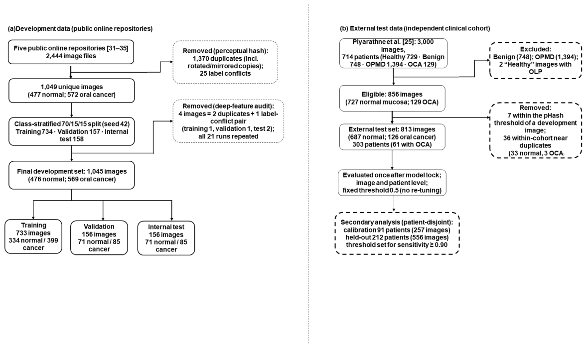
Figure 2.
Analysis pipeline.
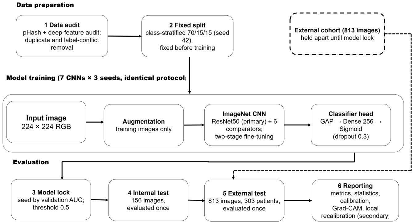
Figure 3.
Training and validation loss (left) and accuracy (right) of the locked ResNet50 run (seed 2). The dashed line marks the start of fine-tuning (stage 2).
Figure 3.
Training and validation loss (left) and accuracy (right) of the locked ResNet50 run (seed 2). The dashed line marks the start of fine-tuning (stage 2).
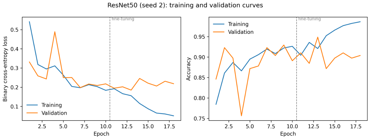
Figure 4.
Internal-test AUC and balanced accuracy of the seven CNNs, mean ± SD over three seeds.
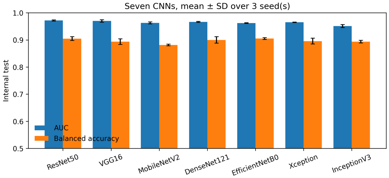
Figure 5.
Receiver operating characteristic curves of the locked models of the seven CNNs on the internal test set. ResNet50 is drawn with a thicker line. AUC values are given in the legend.
Figure 5.
Receiver operating characteristic curves of the locked models of the seven CNNs on the internal test set. ResNet50 is drawn with a thicker line. AUC values are given in the legend.
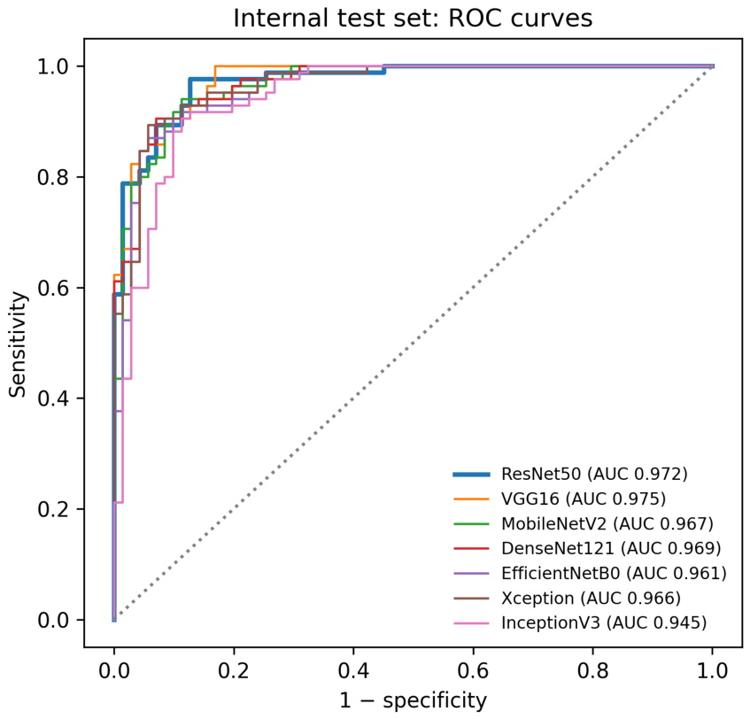
Figure 6.
ROC curves of the locked ResNet50 on the internal test set and on the external cohort at image and patient level.
Figure 6.
ROC curves of the locked ResNet50 on the internal test set and on the external cohort at image and patient level.
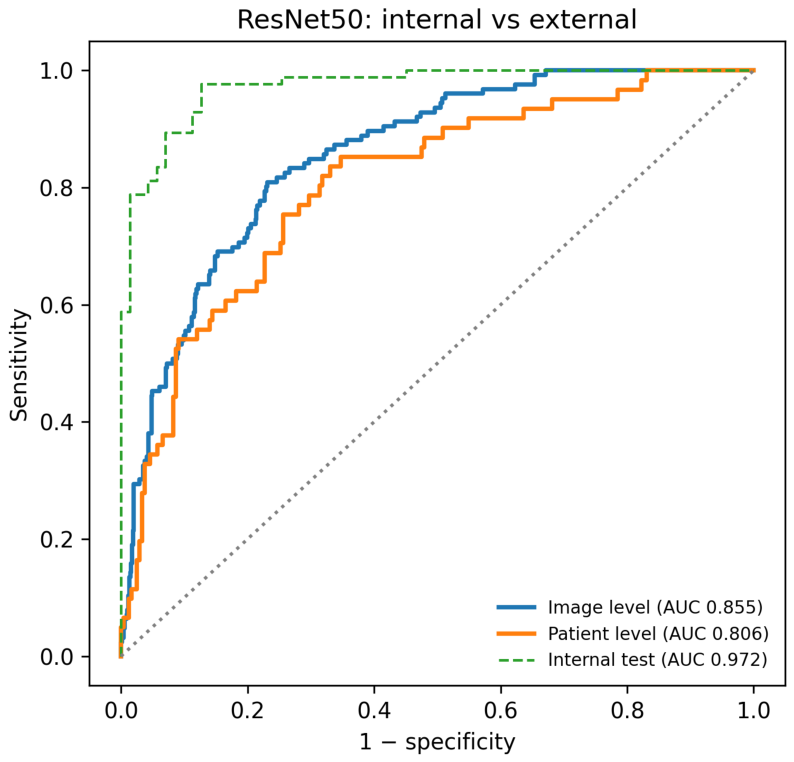
Figure 7.
Confusion matrices of the locked ResNet50 at the prespecified threshold of 0.5 on the internal test set (left) and the external cohort (right) (image level).
Figure 7.
Confusion matrices of the locked ResNet50 at the prespecified threshold of 0.5 on the internal test set (left) and the external cohort (right) (image level).
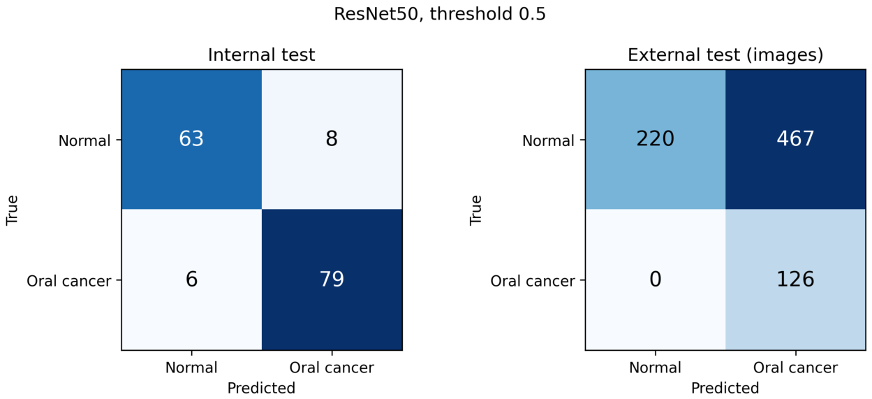
Figure 8.
Reliability diagram of the locked ResNet50 on the internal test set and the external cohort (ten equal-width bins; bins with fewer than five images omitted). The dotted line indicates perfect calibration.
Figure 8.
Reliability diagram of the locked ResNet50 on the internal test set and the external cohort (ten equal-width bins; bins with fewer than five images omitted). The dotted line indicates perfect calibration.
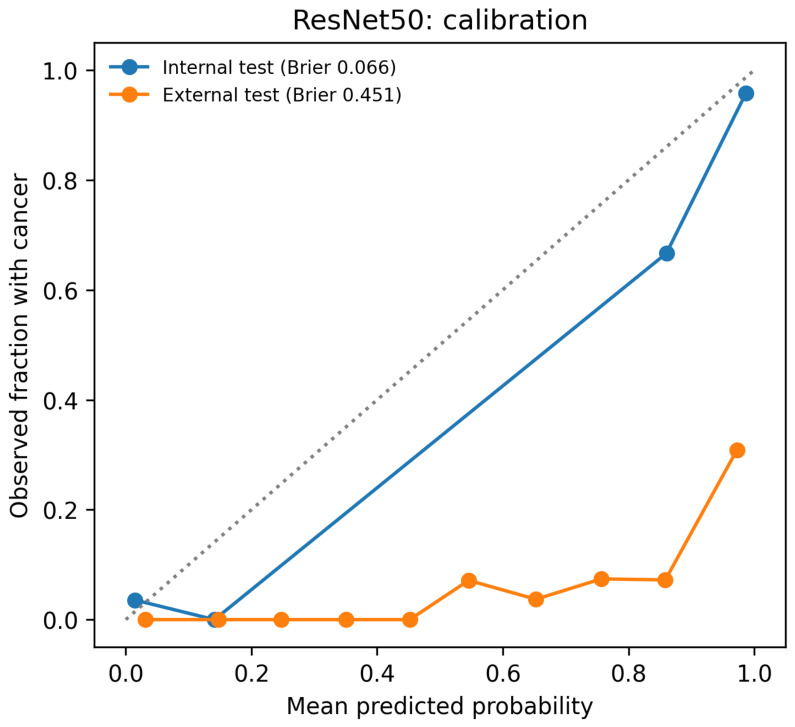
Figure 9.
Grad-CAM maps of the locked ResNet50 for internal-test images (top: input; bottom: overlay), with the predicted probability of oral cancer. Maps were computed for the predicted class from the final residual stage. Qualitative illustration only.
Figure 9.
Grad-CAM maps of the locked ResNet50 for internal-test images (top: input; bottom: overlay), with the predicted probability of oral cancer. Maps were computed for the predicted class from the final residual stage. Qualitative illustration only.
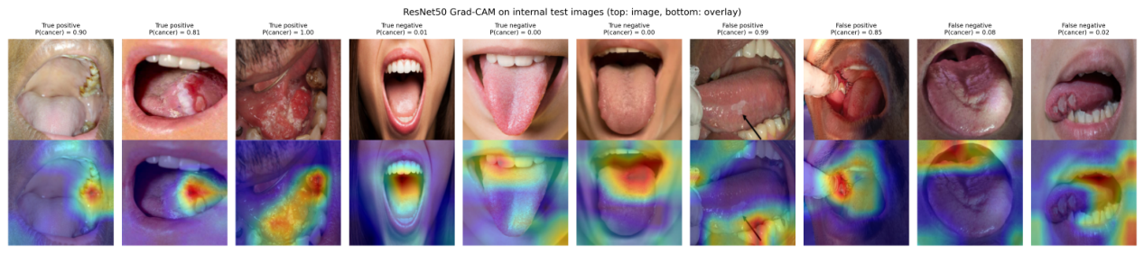
Table 1.
Representative prior work in deep learning for oral lesion / cancer classification.
| Ref. | Imaging / data type | Method / architecture | Task / application | Key strength | Main limitation / gap |
|---|---|---|---|---|---|
| [2] | Clinical oral images | Deep CNN | Detection + classification | Real-world screening relevance | Limited external validation |
| [3] | Clinical oral images | Deep multiclass DL | Multiclass lesion classification | Works under unrestricted image-capture conditions | High deployment complexity |
| [4] | White lesion images | Comparative CNNs | White lesion classification | Strong architecture benchmarking | Narrow lesion scope |
| [5] | Clinical oral photographs | Two-stage detector + CNN classifier | Detection and classification of benign lesions, OPMD, and carcinoma | Automated lesion localisation | Multistage pipeline adds complexity |
| [6] | Clinical oral photographs | DenseNet-169, ResNet-101, Swin-S; Faster R-CNN, YOLOv5 | Classification and detection of OPMD and OSCC | Broad CNN and detector benchmark | Lower detection performance for OPMD |
| [7] | Smartphone oral images | HRNet vs VGG16, ResNet50, DenseNet169 | Four-class oral lesion classification | Multiple smartphone types | Moderate sensitivity (83%) |
| [8] | Clinical oral images | VGG19, DeiT, MobileNet (transfer learning) | Benign vs malignant lesion classification | CNN and transformer comparison | Near-perfect accuracy; independent validation needed |
| [9] | Mobile oral images | Vision Transformer, Swin Transformer vs VGG19 | Oral cancer image classification | Images from high-risk populations | Transformers are data-intensive |
| [10] | Medical images | ResNet50 + VGG16 hybrid | Diagnosis | Improved diagnostic performance | Generic medical task |
| [11] | Clinical oral images | Ensemble ResNet-50 + VGG-16 | Normal vs precancerous lesion classification | Combines complementary CNNs | Binary task only |
| [12] | Oral lesion images | Vision transformer vs radiomics | Oral lesion classification | Global context modeling | Data hungry |
| [13] | Clinical AI systems | Review | Oral surgery support | Broad clinical perspective | Not task-specific |
| [14] | Smartphone images (field) | CNN-enabled mHealth point-of-care device | Screening of OPMD and oral cancer | Field validation with 5,025 subjects | Single-country screening programme |
| [15] | Histopathology images | Hyperparameter-tuned BiGRU | Oral cancer classification | Metaheuristic hyperparameter optimisation | Recurrent design not tailored to spatial image structure |
| [16] | Oral cancer images | RBFNN + metaheuristic optimization | Oral cancer detection and classification | Potential accuracy improvement | Scalability uncertain |
| [17] | Histopathology images | NasNet features + optimised deep belief network | OSCC detection and classification | Metaheuristic hyperparameter tuning | Different imaging modality |
| [18] | Histopathology images | CNN + vision transformer + few-shot | Broad cancer benchmarking | Fair model comparison | High compute cost |
| [19] | Histopathology images | Optimized deep learning | Multiclass classification | Importance of hyperparameter tuning | Proprietary dataset |
| [20] | Histopathology images | Hybrid deep learning | OSCC classification | Rich representation learning | Complex pipeline |
| [26] | Dental images | Dual transformer | Caries diagnosis | Cross-attention learning | High complexity |
| [27] | White lesion photographs | CNNs, transformers, YOLOv7/YOLOv8 | OPMD and white lesion classification and detection | Five-class white-lesion benchmark | Restricted to white lesions |
| [28] | Precancer oral images | Deep learning | Precancer detection | Supports early intervention | Narrow anatomical focus |
| [29] | Oral cancer images | CNN | Cancer detection | Diagnostic automation | Lack of standard benchmarking |
| [30] | Intraoral images | U-Net segmentation + DenseNet201 (mobile app) | OPMD detection and risk stratification | Integrated segmentation-classification app | Small dataset; lower recall for carcinoma |
Table 4.
Training configuration, identical for all seven CNNs.
| Component | Setting |
|---|---|
| Input | 224 × 224 × 3 RGB; bilinear resizing; model-specific ImageNet preprocessing |
| Augmentation (training only) | Horizontal flip; rotation ±15∘; translation ±10%; zoom ±10%; brightness ±10%; reflection padding |
| Classification head | GAP → dropout 0.3 → dense 256 (ReLU) → dropout 0.3 → dense 1 (sigmoid) |
| Stage 1 | Backbone frozen; Adam, learning rate 1 × 10⁻³; ≤ 10 epochs |
| Stage 2 | Top 30% of backbone layers unfrozen (batch normalisation frozen); Adam, 1 × 10⁻⁵; ≤ 40 epochs |
| Loss and class imbalance | Binary cross-entropy with balanced class weights (normal 1.097; oral cancer 0.919) |
| Batch size | 16 |
| Early stopping | Validation loss; patience 5; best weights restored |
| Learning-rate schedule | × 0.5 after 2 epochs without validation-loss improvement; minimum 1 × 10⁻⁷ |
| Seeds | 0, 1, 2 (Python, NumPy, TensorFlow) |
| Checkpoint and seed selection | Checkpoint: lowest validation loss (early stopping, best weights restored); seed: highest validation AUC per model (ties: validation balanced accuracy) |
| Decision threshold | 0.5, fixed in advance; not re-tuned on any test set |
| Software and hardware | Python 3.13.15, TensorFlow 2.20.0, Keras 3.13.2, NumPy 2.1.3; Google Colab, NVIDIA Tesla T4 GPU |
Table 5.
Validation results (156 images) used for seed selection.
| Model | Validation AUC, mean ± SD (3 seeds) | Validation balanced accuracy, mean (3 seeds) | Locked seed |
|---|---|---|---|
| ResNet50 | 0.976 ± 0.002 | 0.937 | 2 |
| VGG16 | 0.985 ± 0.004 | 0.933 | 1 |
| MobileNetV2 | 0.959 ± 0.007 | 0.904 | 0 |
| DenseNet121 | 0.968 ± 0.002 | 0.912 | 2 |
| EfficientNetB0 | 0.963 ± 0.007 | 0.908 | 0 |
| Xception | 0.968 ± 0.001 | 0.912 | 1 |
| InceptionV3 | 0.960 ± 0.002 | 0.892 | 2 |
For each model, the locked seed is the seed that produced the highest validation AUC. This selection was entered in the lock file (23 September 2026, 10:21:55) before any test metric was calculated.
Table 6.
Internal test performance, mean ± SD over three seeds.
| Model | Accuracy | Balanced accuracy | Sensitivity | Specificity | F1 | AUC | |
|---|---|---|---|---|---|---|---|
| ResNet50 | 0.906 ± 0.007 | 0.905 ± 0.007 | 0.918 ± 0.012 | 0.892 ± 0.008 | 0.914 ± 0.007 | 0.972 ± 0.002 | 0.810 ± 0.015 |
| VGG16 | 0.891 ± 0.011 | 0.894 ± 0.011 | 0.863 ± 0.018 | 0.925 ± 0.008 | 0.896 ± 0.011 | 0.970 ± 0.005 | 0.782 ± 0.022 |
| MobileNetV2 | 0.876 ± 0.004 | 0.881 ± 0.003 | 0.824 ± 0.012 | 0.939 ± 0.008 | 0.879 ± 0.005 | 0.963 ± 0.004 | 0.753 ± 0.007 |
| DenseNet121 | 0.897 ± 0.013 | 0.900 ± 0.012 | 0.871 ± 0.024 | 0.930 ± 0.000 | 0.902 ± 0.013 | 0.967 ± 0.002 | 0.795 ± 0.025 |
| EfficientNetB0 | 0.902 ± 0.004 | 0.905 ± 0.003 | 0.867 ± 0.007 | 0.944 ± 0.000 | 0.906 ± 0.004 | 0.962 ± 0.001 | 0.803 ± 0.007 |
| Xception | 0.893 ± 0.010 | 0.896 ± 0.011 | 0.867 ± 0.007 | 0.925 ± 0.022 | 0.898 ± 0.009 | 0.965 ± 0.001 | 0.786 ± 0.020 |
| InceptionV3 | 0.895 ± 0.004 | 0.894 ± 0.005 | 0.910 ± 0.014 | 0.878 ± 0.022 | 0.904 ± 0.003 | 0.951 ± 0.006 | 0.789 ± 0.008 |
Threshold 0.5. Oral cancer is the positive class. SD of 0.000 indicates identical values in all three seeds.
Table 7.
Internal test performance of the locked model of each architecture, with 95% confidence intervals.
Table 7.
Internal test performance of the locked model of each architecture, with 95% confidence intervals.
| Model | Accuracy | Balanced accuracy | Sensitivity | Specificity | F1 | AUC | TN / FP / FN / TP | |
|---|---|---|---|---|---|---|---|---|
| ResNet50 | 0.910 (0.855–0.946) | 0.908 (0.859–0.951) | 0.929 (0.854–0.967) | 0.887 (0.793–0.942) | 0.919 (0.870–0.957) | 0.819 (0.718–0.906) | 0.972 (0.952–0.993) | 63 / 8 / 6 / 79 |
| VGG16 | 0.885 (0.825–0.926) | 0.887 (0.835–0.933) | 0.859 (0.769–0.917) | 0.915 (0.828–0.961) | 0.890 (0.836–0.936) | 0.769 (0.664–0.859) | 0.975 (0.956–0.994) | 65 / 6 / 12 / 73 |
| MobileNetV2 | 0.878 (0.818–0.921) | 0.884 (0.835–0.928) | 0.824 (0.729–0.890) | 0.944 (0.864–0.978) | 0.881 (0.824–0.927) | 0.758 (0.646–0.846) | 0.967 (0.943–0.991) | 67 / 4 / 15 / 70 |
| DenseNet121 | 0.910 (0.855–0.946) | 0.912 (0.863–0.955) | 0.894 (0.811–0.943) | 0.930 (0.846–0.970) | 0.916 (0.865–0.957) | 0.820 (0.718–0.908) | 0.969 (0.947–0.991) | 66 / 5 / 9 / 76 |
| EfficientNetB0 | 0.904 (0.847–0.941) | 0.907 (0.861–0.949) | 0.871 (0.783–0.926) | 0.944 (0.864–0.978) | 0.908 (0.859–0.950) | 0.808 (0.714–0.897) | 0.961 (0.934–0.989) | 67 / 4 / 11 / 74 |
| Xception | 0.904 (0.847–0.941) | 0.907 (0.859–0.949) | 0.871 (0.783–0.926) | 0.944 (0.864–0.978) | 0.908 (0.855–0.951) | 0.808 (0.706–0.897) | 0.966 (0.941–0.990) | 67 / 4 / 11 / 74 |
| InceptionV3 | 0.891 (0.832–0.931) | 0.888 (0.835–0.936) | 0.918 (0.840–0.960) | 0.859 (0.760–0.922) | 0.902 (0.848–0.944) | 0.780 (0.675–0.872) | 0.945 (0.910–0.981) | 61 / 10 / 7 / 78 |
CIs: Wilson (accuracy, sensitivity, specificity), DeLong (AUC), percentile bootstrap with 2,000 resamples (balanced accuracy, F1, ). TN, true negatives; FP, false positives; FN, false negatives; TP, true positives.
Table 8.
Paired comparison of ResNet50 with each comparator on the internal test set.
| Comparator | AUC (ResNet50 − comparator) | DeLong p | DeLong p (Holm) | b | c | McNemar p | McNemar p (Holm) |
|---|---|---|---|---|---|---|---|
| VGG16 | −0.002 | 0.656 | 1.000 | 8 | 4 | 0.388 | 1.000 |
| MobileNetV2 | 0.005 | 0.575 | 1.000 | 12 | 7 | 0.359 | 1.000 |
| DenseNet121 | 0.004 | 0.643 | 1.000 | 6 | 6 | 1.000 | 1.000 |
| EfficientNetB0 | 0.011 | 0.202 | 1.000 | 7 | 6 | 1.000 | 1.000 |
| Xception | 0.007 | 0.421 | 1.000 | 8 | 7 | 1.000 | 1.000 |
| InceptionV3 | 0.027 | 0.041 | 0.245 | 9 | 6 | 0.607 | 1.000 |
b, images classified correctly by ResNet50 only; c, images classified correctly by the comparator only. Exact (binomial) McNemar test at threshold 0.5; Holm adjustment across the six comparisons.
Table 9.
External validation at image level (813 images, 303 patients).
| Model | Balanced accuracy | Sensitivity | Specificity | PPV | NPV | AUC | Brier | TN / FP / FN / TP |
|---|---|---|---|---|---|---|---|---|
| ResNet50 | 0.660 (0.637–0.684) | 1.000 (0.970–1.000)a | 0.320 (0.274–0.368) | 0.212 (0.151–0.276) | 1.000 (0.983–1.000)a | 0.855 (0.808–0.893) | 0.451 | 220 / 467 / 0 / 126 |
| VGG16 | 0.719 (0.673–0.755) | 0.905 (0.832–0.955) | 0.533 (0.479–0.584) | 0.262 (0.184–0.342) | 0.968 (0.946–0.986) | 0.855 (0.797–0.901) | 0.327 | 366 / 321 / 12 / 114 |
| MobileNetV2 | 0.683 (0.640–0.720) | 0.929 (0.857–0.984) | 0.438 (0.389–0.485) | 0.233 (0.164–0.305) | 0.971 (0.942–0.994) | 0.820 (0.753–0.871) | 0.369 | 301 / 386 / 9 / 117 |
| DenseNet121 | 0.678 (0.644–0.707) | 0.952 (0.906–0.988) | 0.403 (0.352–0.453) | 0.226 (0.160–0.296) | 0.979 (0.960–0.994) | 0.839 (0.780–0.887) | 0.375 | 277 / 410 / 6 / 120 |
| EfficientNetB0 | 0.768 (0.725–0.804) | 0.905 (0.836–0.957) | 0.630 (0.577–0.682) | 0.310 (0.224–0.395) | 0.973 (0.951–0.990) | 0.858 (0.815–0.897) | 0.248 | 433 / 254 / 12 / 114 |
| Xception | 0.680 (0.650–0.708) | 0.960 (0.922–0.991) | 0.399 (0.348–0.446) | 0.227 (0.161–0.294) | 0.982 (0.964–0.996) | 0.824 (0.768–0.869) | 0.399 | 274 / 413 / 5 / 121 |
| InceptionV3 | 0.613 (0.582–0.637) | 0.952 (0.904–0.987) | 0.274 (0.235–0.310) | 0.194 (0.134–0.256) | 0.969 (0.942–0.991) | 0.780 (0.718–0.830) | 0.477 | 188 / 499 / 6 / 120 |
Locked models, threshold 0.5, no re-tuning. 95% CIs from a patient-cluster bootstrap (2,000 resamples of patients). a The bootstrap interval collapses to 1.000–1.000 when no errors occur, so the Wilson interval is shown instead. PPV, positive predictive value; NPV, negative predictive value.
Table 10.
External validation at patient level (303 patients; 61 with OCA).
| Model | Balanced accuracy | Sensitivity | Specificity | AUC | TN / FP / FN / TP |
|---|---|---|---|---|---|
| ResNet50 | 0.583 (0.560–0.606) | 1.000 (0.941–1.000) | 0.165 (0.124–0.217) | 0.806 (0.745–0.868) | 40 / 202 / 0 / 61 |
| VGG16 | 0.651 (0.605–0.693) | 0.934 (0.843–0.974) | 0.368 (0.310–0.430) | 0.821 (0.758–0.884) | 89 / 153 / 4 / 57 |
| MobileNetV2 | 0.589 (0.548–0.627) | 0.934 (0.843–0.974) | 0.244 (0.194–0.302) | 0.759 (0.691–0.826) | 59 / 183 / 4 / 57 |
| DenseNet121 | 0.593 (0.553–0.630) | 0.951 (0.865–0.983) | 0.236 (0.186–0.293) | 0.814 (0.750–0.877) | 57 / 185 / 3 / 58 |
| EfficientNetB0 | 0.709 (0.669–0.747) | 0.967 (0.888–0.991) | 0.450 (0.389–0.513) | 0.845 (0.797–0.894) | 109 / 133 / 2 / 59 |
| Xception | 0.593 (0.558–0.625) | 0.967 (0.888–0.991) | 0.219 (0.172–0.275) | 0.747 (0.676–0.818) | 53 / 189 / 2 / 59 |
| InceptionV3 | 0.529 (0.488–0.567) | 0.918 (0.822–0.964) | 0.140 (0.102–0.190) | 0.703 (0.624–0.782) | 34 / 208 / 5 / 56 |
Table 11.
Fixed versus locally recalibrated thresholds on the held-out external patients (212 patients, 556 images; 81 oral cancer).
Table 11.
Fixed versus locally recalibrated thresholds on the held-out external patients (212 patients, 556 images; 81 oral cancer).
| Model | Threshold | Sensitivity | Specificity | Balanced accuracy | PPV | NPV |
|---|---|---|---|---|---|---|
| ResNet50 | Fixed (0.500) | 1.000 (0.955–1.000)a | 0.322 (0.266–0.382) | 0.661 (0.633–0.691) | 0.201 (0.134–0.281) | 1.000 (0.976–1.000)a |
| Recalibrated (0.946) | 0.790 (0.698–0.867) | 0.756 (0.703–0.804) | 0.773 (0.721–0.818) | 0.356 (0.237–0.487) | 0.955 (0.928–0.976) | |
| VGG16 | Fixed (0.500) | 0.901 (0.818–0.959) | 0.549 (0.483–0.617) | 0.725 (0.671–0.768) | 0.254 (0.166–0.357) | 0.970 (0.946–0.989) |
| Recalibrated (0.689) | 0.889 (0.797–0.954) | 0.640 (0.576–0.704) | 0.764 (0.710–0.807) | 0.296 (0.193–0.411) | 0.971 (0.951–0.988) | |
| MobileNetV2 | Fixed (0.500) | 0.951 (0.875–1.000) | 0.455 (0.394–0.511) | 0.703 (0.655–0.741) | 0.229 (0.150–0.322) | 0.982 (0.956–1.000) |
| Recalibrated (0.479) | 0.963 (0.890–1.000) | 0.448 (0.387–0.504) | 0.706 (0.660–0.742) | 0.229 (0.151–0.321) | 0.986 (0.962–1.000) | |
| DenseNet121 | Fixed (0.500) | 0.951 (0.887–0.990) | 0.404 (0.339–0.467) | 0.677 (0.633–0.715) | 0.214 (0.140–0.300) | 0.980 (0.956–0.996) |
| Recalibrated (0.766) | 0.864 (0.776–0.935) | 0.617 (0.552–0.681) | 0.741 (0.690–0.787) | 0.278 (0.185–0.386) | 0.964 (0.936–0.985) | |
| EfficientNetB0 | Fixed (0.500) | 0.938 (0.885–0.981) | 0.638 (0.573–0.699) | 0.788 (0.748–0.826) | 0.306 (0.212–0.414) | 0.984 (0.967–0.997) |
| Recalibrated (0.380) | 0.951 (0.900–0.989) | 0.581 (0.511–0.648) | 0.766 (0.724–0.805) | 0.279 (0.192–0.380) | 0.986 (0.970–0.997) | |
| Xception | Fixed (0.500) | 0.951 (0.894–0.990) | 0.406 (0.348–0.465) | 0.678 (0.637–0.714) | 0.214 (0.142–0.300) | 0.980 (0.955–0.996) |
| Recalibrated (0.885) | 0.778 (0.644–0.878) | 0.697 (0.639–0.754) | 0.737 (0.661–0.796) | 0.304 (0.192–0.426) | 0.948 (0.918–0.974) | |
| InceptionV3 | Fixed (0.500) | 0.938 (0.864–0.986) | 0.282 (0.232–0.332) | 0.610 (0.569–0.647) | 0.182 (0.117–0.261) | 0.964 (0.928–0.992) |
| Recalibrated (0.764) | 0.889 (0.800–0.954) | 0.484 (0.423–0.541) | 0.687 (0.634–0.733) | 0.227 (0.146–0.324) | 0.962 (0.935–0.985) |
Secondary analysis. Recalibrated thresholds were set on 91 separate calibration patients (257 images) as the highest threshold giving a sensitivity ≥ 0.90; model weights were unchanged. Values are point estimates with 95% CIs from a patient-cluster bootstrap (2,000 resamples of patients). a The bootstrap interval collapses to 1.000–1.000 when no errors occur, so the Wilson interval is shown instead.
Disclaimer/Publisher’s Note: The statements, opinions and data contained in all publications are solely those of the individual author(s) and contributor(s) and not of MDPI and/or the editor(s). MDPI and/or the editor(s) disclaim responsibility for any injury to people or property resulting from any ideas, methods, instructions or products referred to in the content. |
© 2026 by the authors. Licensee MDPI, Basel, Switzerland. This article is an open access article distributed under the terms and conditions of the Creative Commons Attribution (CC BY) license (http://creativecommons.org/licenses/by/4.0/).
Copyright: This open access article is published under a Creative Commons CC BY 4.0 license, which permit the free download, distribution, and reuse, provided that the author and preprint are cited in any reuse.