

Submitted:
14 November 2026
Posted:
16 November 2026
You are already at the latest version
Abstract
The paper develops one idea: the appearance of a new discrete eigenvalue of an operator built from a flow is a qualitative event in the flow. \emph{Part I (theory).} For the three-dimensional Navier-Stokes equations with a force in divergence form we give a short proof of global regularity when \(E_0Y_0 \lesssim \frac{27}{256\pi^4}v^4 \approx 0.642^4v^4\), a scale-invariant small-data condition with an explicit, not optimal, constant. Treating the velocity as the potential, \(-c|v|^2/v^2\), we prove that a finite-time singularity makes the Schrödinger operator bind for couplings \(c\) above a threshold, that the absence of bound states is a bound on a multiplier norm of \(v\), and that the first threshold is preceded by the divergence of the zero-energy scattering amplitude. The spectral data obey an explicit evolution identity, which is not closed: \(v\) and \(-v\) give the same operator and, in a computed example, different evolutions. The author's scattering representation of the potential is put into normalised form, with its conditional status stated. Part II (realization). In inviscid stability problems the operator is fixed by the flow, and for the classical class of profiles, a bound state is an unstable mode. We compute this for shear layers, jets, a current sheet, vortices and a Rayleigh-Taylor layer, and show that the threshold is predicted from the stable side by the growth of a response. For Taylor vortices the viscous threshold is the lowest neutral eigenvalue of a sixth-order operator with Rayleigh's discriminant as potential, and the standard critical Reynolds number is recovered. Followed through the nonlinear stage, the amplitude of the vortex approaches a square-root law at the threshold (shear layer, Taylor vortices); the pressure changes continuously in an incompressible fluid, and in our compressible runs at convective Mach numbers 0.7 and 0.8 the birth of the vortex ends in a shock. With a free constant the operator measures intensity only. For the forced construction announced by OpenAI in 2026, if its stated asymptotics hold, the operator binds for every coupling. The picture does not apply to subcritical transition, and no result here bears on the Millennium problem.
Keywords:
Navier–Stokes equations
; small data
; scaling invariance
; inverse scattering
; bound states
; Birman–Schwinger principle
; hydrodynamic stability
; vortex
; Taylor vortices
MSC: 35Q30; 76D05; 35B65; 35P25
1. Introduction
We study the Cauchy problem
in , , with viscosity and .
In Fefferman’s formulation of the Millennium Prize Problem [45] the statements (A) and (B) concern global regularity without force, on and on the torus, while (C) and (D) concern breakdown of smooth solutions under a smooth force. In September 2026 OpenAI announced a construction for (C) and (D) [61]: for every there are a force and a smooth solution with whose velocity is unbounded as . The construction has not yet been independently verified, and the formal (Lean) version has been reported not to match the written proof [4]. Constantin, Ignatova and Vicol proved a conditional local regularity theorem for asymptotically axisymmetric solutions with spatially analytic forcing [38]; applied to the properties stated for the construction, it shows that the force cannot be real-analytic near the singular point.
This raises a natural question: what relation between and f guarantees global regularity? The answer has to be invariant under the scaling of (1). For fixed the equations are preserved by
and a smallness condition on a quantity that scales with a non-zero power of can always be achieved by rescaling, so it cannot by itself guarantee regularity. In earlier work [39,40] the author used an amplitude–time rescaling , , . This transformation only multiplies (1) by and leaves the Reynolds number unchanged, so it cannot produce smallness by itself. In the present paper smallness comes instead from an explicit invariant condition. A conditional global existence result of a different, abstract type was obtained in [62].
We stress that we do not claim progress on statements (A)–(D). Our condition is a smallness condition; by Remark 2 it implies smallness of the data in the critical space , under which global regularity is classical [44,50,58]. What the paper adds here is the explicit constant in the classical energy argument, the treatment of a force in divergence form, and the resulting quantitative obstruction for forces that produce singularities. The threshold uses the sharp Sobolev constant; we do not claim that the threshold itself is optimal.
The point of view.
The paper is organised around one idea: the appearance of a new discrete eigenvalue of a Schrödinger operator built from the flow is a qualitative event in the flow. In Part I the operator is , and the theorems say that a singularity of the Navier–Stokes equations forces this operator to bind, that the first binding is preceded by the divergence of the zero-energy scattering amplitude, and that the spectral data do not obey a closed evolution law. In Part II the operator is the one that linear stability theory attaches to a given flow, with no free constant; there a new discrete state is a new unstable mode, and its nonlinear outcome is a new structure, a vortex. Part II checks this by direct computation, including the law by which a vortex is born, and states where the picture does not apply. The reduction of stability problems to Schrödinger operators is classical, and so is the statement that, for the classical class of profiles, a bound state of the reduced operator is an unstable mode (the neutral-mode method of Tollmien, Lin and Howard; [5,6]). What is added here is narrower: the prediction of the threshold from the stable side through a response, the collected quantitative checks, and the measurements of the nonlinear amplitude of the vortex.
All statements about the construction of [61] are conditional on its correctness: Corollary 1, Corollary 3, Remark 14 and Section 14. The rest of the paper does not depend on it.
Main results.
Part I. Theorem 1 gives global regularity under the dominance condition (D); Proposition 1 records the classical local existence time with an explicit constant; Corollary 1 gives a lower bound that every force producing a singularity must satisfy. Section 4 puts the representation of the potential through the scattering data [43] into normalised form and says which of its statements are proved and which are conditional (Remark 7). Section 5 contains the spectral theorems for : binding before a singularity (Theorems 5 and 9), the count of bound states (Theorem 10, conditional on a cited statement) and the divergence of the zero-energy amplitude (Theorem 6). Section 6 and Section 7 give the trace formulas and the absence of a closed evolution law (Proposition 9); Section 8 treats two dimensions. Part II. Section 9 computes the stability examples in which the operator has no free constant; Section 10 follows the birth of a vortex through the nonlinear stage, with the pressure in the incompressible and compressible cases; Section 11 treats vortices, including Taylor vortices step by step; Section 12 adds the round jet; Section 13 gives three-dimensional and stratified cases, with a map of the classical problems (Table 2). Section 14 analyses the construction of [61], conditionally on its announced asymptotics, and Section 15 tests the operator with a free constant in convection and reduced MHD. The statements of Part II, except Proposition 11, are computations for particular flows and not theorems; their accuracy is stated where they appear.
- Part I. Theory
2. Notation and Standard Facts
We write for the norm of and for its inner product. The following inequalities hold for divergence-free fields in .
- Interpolation: by Hölder’s inequality, and on . Hence
- Integration by parts: .
Combining the Sobolev inequality with (3) and Hölder’s inequality gives
Definition 1.
- (F1)
- For such data there is a unique strong solution on a maximal interval , and . If , then as .
- (F2)
- For a strong solution, the identities obtained by testing (1) with v and with hold for a.e. t. The pressure drops out because v and are divergence free.
- (F3)
- A strong solution is unique in the class of Leray–Hopf weak solutions with the same data (weak–strong uniqueness). If the data are smooth with the decay required in [45], the solution is smooth on .
- (F4)
3. Main Result
Let the force have the form
Every has this form with , and then ; this choice minimises among all representations of f, and the quantity below depends on the representation chosen. So (5) means that the force is a sum of derivatives of fields whose size enters the condition below. We set
Theorem 1
Lemma 1
(Energy). Every strong solution on satisfies (7) for .
Lemma 2
(Enstrophy under dominance). Let v be a strong solution on and let . If
then (8) holds on .
Proof.
Proof of Theorem 1.
Let v be the maximal strong solution on given by (F1). Since by (F1), the function is continuous, and the set
is a relatively closed subinterval of . It contains 0, because . For , Lemmas 1 and 2 give
by (D). So the inequality defining S is strict on S, and by continuity S is also open in . Hence , and (8) holds on . Then stays bounded, and (F1) gives . Uniqueness and smoothness follow from (F3). □
Remark 1
(Scaling and dimension). Under (2) with one has and . So the product is invariant. Dimensionally , so is dimensionless, the fourth power of a Reynolds-type number. Condition (D) is therefore one explicit, scale-invariant sufficient form of the statement “viscosity dominates the force”. For , condition (D) reduces to Leray’s classical smallness of relative to [59]. The divergence form (5) lets the energy-level part of the force be measured in , one derivative below .
Remark 2
(Relation to critical small-data theory). By Plancherel’s theorem and the Cauchy–Schwarz inequality, and . A further Cauchy–Schwarz inequality gives
Hence (D) implies smallness of the data, relative to , in the critical space , and global regularity then also follows from the Fujita–Kato theory with forcing [44,58]. Theorem 1 should be read as an -level proof of a special case of that theory, with an explicit (not optimal) threshold and the bounds (7)–(8).
Remark 3
Proposition 1
(Classical local existence time). Let , , , , and let be defined by (6). Then the strong solution exists at least on with
(if then and ). This is the classical local result; regularity on an arbitrary finite interval without smallness is the open problem itself.
Proof.
Apply Young’s inequality to (4): . Together with the bound for the force term used above this gives
As long as we get , and this is strictly less than for . A continuity argument and (F1) complete the proof. □
Corollary 1
(Lower bound for singular forces). Let v be the strong solution of (1) with maximal time (equivalently, by (F1), as ), and let the force satisfy (5) on . Then
In particular, suppose the construction of [61] is correct: , , and a solution that is smooth with compact spatial support on and has unbounded velocity as . Such a solution is a strong solution on every , , hence by (F3) it is the strong solution; its maximal time is 1, because a strong solution with a smooth compactly supported force is bounded on compact subintervals of its interval of existence. Its force then satisfies
The finite-energy hypothesis matters: without decay, smooth solutions on are not unique (e.g. , ).
Proof.
The proof of Theorem 1 works on with the integrals in (6) taken over . If the inequality failed, it would give on , contradicting (F1). In , every lies in . □
4. The Velocity as a Potential: a Scattering Representation and Its Limits
In [39,40,41,42] the author proposed to estimate the velocity by treating its components as potentials of the Schrödinger operator and recovering the potential from the scattering data through the Poincaré–Riemann–Hilbert problem. The analytic part of this programme is developed in the manuscript [43], which has not yet been refereed. In this section we put the representation into the normalized form required by the Riemann–Hilbert problem. We check it in the Born approximation, identify its leading term, and state what it gives for the Navier–Stokes equations.
Setting and status of the statements.
Throughout this section are the Cauchy projectors in the spectral variable, , so that and for g analytic and decaying in the lower half-plane. The identities below are proved for potentials q in the Schwartz class with , for real , and are understood in the sense of distributions in x; for such q the Neumann series of the Lippmann–Schwinger equation converges uniformly in the closed half-plane, which gives the a priori bound used in Lemma 3. The condition already excludes bound states. Whenever the series (11) is used, we assume that it converges to . Theorem 3 is an identity that holds when the integrals in it converge absolutely, and Corollary 2 is conditional on a high-energy bound that we do not prove. No estimate of the velocity is obtained in this section.
The normalized Riemann–Hilbert representation
Let q be a real potential of Rollnik class on , and let , , be the outgoing and incoming solutions of with incident wave . Let be the scattering amplitude, normalized so that in the Born approximation with . Put
Remark 4
(Two corrections to the setting of [43]). Normalization. The Cauchy operators in k must be applied to μ, not to Φ. The phase in the Lippmann–Schwinger equation for is bounded in the lower half-plane, and that for in the upper half-plane, and there. In contrast, grows in one of the half-planes, so the Cauchy formula does not hold for . Scale invariance. The smallness condition of [43, Lemma 1] adds quantities of different dimensions (length and length−1/2). It depends on the unit of length and is not invariant under . Since for real k, the series is controlled by the Kato norm , which is dimensionless and scale invariant. In units where the splitting radius is 1, .
Lemma 3.
If , then . In particular, for .
Proof.
, so , and therefore . □
This is where the threshold of [43] enters naturally. On the real axis, , and the classical relation between and [72] gives the Riemann–Hilbert problem
For the amplitude is defined by , which for real q is forced by the symmetry of the outgoing and incoming solutions. Under a smallness condition on the amplitude of the type of [43, Lemma 5], and assuming that the Riemann–Hilbert problem is uniquely solvable and the series converges in , this gives
The constant in is fixed by the Born approximation: with it, coincides with the first Born term , . Indeed, , and only the exponent survives. With the constant used in [43] the first term is off by the factor .
Example 1
(Why the estimate must be homogeneous). In [43, Theorem 5] the estimate is stated as with , . Its terms have different dimensions, and it fails on concentrating potentials. Take (the amplitude constant set to 1 in units of length), . Then and , while a computation with the Dawson function gives . The right-hand side stays bounded and the left-hand side tends to infinity. A correct pointwise estimate must grow like on this family, that is, it must contain the full Fourier-inversion weight. This is exactly what the leading term below does.
The leading term is the fixed-angle Born approximation
Let . The Schrödinger equation for becomes
an exact identity for every k and . This is the normalized form of the representation of [43]. We insert (11).
Lemma 4
(Removal of the Cauchy kernel). With ,
Consequently the Cauchy kernel in is removed exactly:
which does not depend on k.
Proof.
For we have and . Hence (we checked this symbolically). Then , and multiplying by gives the formula. □
Proposition 2
(The Born check). For fixed θ, the map from to is a bijection up to null sets, with . Hence in the Born approximation
exactly. On the half-space (that is, ), coincides with the inverse fixed-angle Born approximation of Ruiz [77] and Meroño [71]. On the other half-space they use data with incident direction , while uses ; by unitarity the two differ by a term quadratic in the data.
Proof.
The identity of Lemma 4 holds in the sense of distributions; pointwise it requires , that is, an amplitude integrable in . The set is the unit sphere centred at , which passes through the origin. Each ray from the origin meets it once more, at a point p with , and this determines s uniquely, including its sign. In spherical coordinates about , the area element and the factor give the Jacobian . Then . (We also checked the identity numerically for a Gaussian.) □
Theorem 2
(Representation of the potential). Assume that , that has no bound states, and that the series (11) converges. Then for every k and θ
and
Taken alone, the bound in Theorem 2 carries no information beyond , because by definition. It becomes an estimate only if is bounded independently, through the scattering data.
Remark 5
(What is gained and what is not). The leading term carries the full Fourier-inversion weight , which is exactly the Jacobian of . So no derivative is gained in it, in agreement with Example 1. For compactly supported , Meroño [71] proved that the difference between q and his fixed-angle Born approximation is more regular than q, by up to one derivative in the Sobolev scale for and less for , and that more than one derivative cannot be gained in general. Because of the half-space difference noted in Proposition 2, this does not transfer verbatim to . The remainder isnotsmoother than q: its first part has exactly the singularities of q, since is continuous and in general nonzero. For example, at and second order, for the indicator of a ball, jumps across the sphere just as q does. For the phase of a chain is , and produces . Estimating these terms through the scattering data, in the spirit of the double dispersion operator of [71], is what an application would require.
The nonlinear part through the scattering data
The remainder splits as . The first part is trivial, and the content lies in . We now express this difference exactly through the scattering data and , without using the series.
Lemma 5
(Commutation of with the jump operator). Let and . For every smooth ,
where . Consequently, for ,
Proof.
The first identity follows from the product rule, with (we checked it symbolically with sympy for a generic g). In the Cauchy integral the factor cancels the kernel, , and . □
Theorem 3
(Exact formula for the nonlinear part). Under the assumptions of Theorem 2, for every ,
In particular is at least of second order in the scattering data, and .
Proof.
Proposition 3
(Second-order check against Meroño’s formula). Let . At second order in q, Theorem 3 states . Here is built from the Born amplitude, is the first Born term of , and is the second-order part of . For every q in the Schwartz class,
On the half-space this is minus the double dispersion term of [71, Prop. 2.3], including the prescription and the normalization. So the identity holds at second order. On the real (principal-value) parts agree, and the terms have opposite signs. This is the quadratic unitarity difference between and Meroño’s approximation noted after Proposition 2.
Proof.
In Fourier variables , the incoming resolvent shifted by . Also becomes multiplication by , and with . Change variables with (Proposition 2). Then , , and . With , the bracket divided by equals . The denominator, multiplied by , equals after renaming . We verified both algebraic identities symbolically. Tracking gives the stated prescription. □
Theorem 3 is the independent description of the nonlinear part asked for in Remark 5. The difference between the potential and its fixed-angle Born approximation is a bilinear expression in the amplitude and in , and is itself determined by the data through (10). It holds for each and does not involve k. It does not require the series (11), only the Riemann–Hilbert relation and the Schrödinger equation, and it holds wherever the integrals converge. The smoothing results of [71] concern exactly this difference.
Corollary 2
(Estimate of the nonlinear part). Put
and assume the high-energy bound . Then, for ,
Proof.
Use (Lemma 3) in the first term of and the bound on in the second. □
Remark 6
(Dimensions, convergence and what remains). By Proposition 2, is the norm of the amplitude in the momentum variable η. It has the dimension of a potential, and in the Born approximation it equals . is dimensionless, γ has the dimension of a potential, and both sides of the corollary are length−2. The quantity is finite for nice potentials. In the Born approximation behaves like , which is integrable on . The hypothesis on expresses the high-energy behaviour (cf. [72]), which comes from stationary phase in the Lippmann–Schwinger integral and needs some smoothness of q. The crude bound , obtained by differentiating the kernel, grows in s. With it the second term diverges near the forward direction, since . The decay is therefore essential. From the leading high-energy term , one expects for near θ, plus a contribution of ray integrals weighted by . Hence the second term is of the form . The first part can be absorbed when is small. The second involves one derivative of q along rays. Under these assumptions,
Under these unproved assumptions this would be an estimate of the potential through the scattering data, with a nonlinear part of relative size κ and ; note that its right-hand side contains a norm of along rays, which is stronger than . For the Navier–Stokes velocity, however, the free coupling makes κ and small at no cost (Remark 7), so by itself the estimate again reduces to Fourier inversion of the velocity. A rigorous high-energy bound with explicit constants is the remaining step for the scattering theory itself.
The Kato norm along the trajectory
The smallness of the Kato norm requires control of , which the energy inequality does not give directly. It is nevertheless controlled along the trajectory. Let be the kernel of (the Oseen kernel). It satisfies [70,73], hence with absolute constants .
Lemma 6
Proof.
Use Duhamel’s formula . The heat semigroup is a contraction on , which handles and , and the Oseen kernel bound handles the nonlinear term. Moreover , since . This gives the first inequality, and gives the second. If , then is bounded uniformly in t. □
Both sides have the dimension length4/time. Only the energy enters, so the lemma also holds for Leray–Hopf weak solutions.
Lemma 7
(Kato norm through and ). For every ,
Proof.
Split at . This gives , and the minimum over is the stated value. The second inequality is Hölder’s inequality. □
Proposition 5.
Let v be the strong solution of (1) with maximal time , with data as in Lemma 6, and let be as there. Fix . If
then for all and :
- (i)
- ;
- (ii)
- has no bound states;
The smallness here is obtained by choosing the free coupling depending on the data, not from smallness of the data themselves. What is really used is a bound, uniform in time, on .
Proof.
Remark 8
(The OpenAI construction). Proposition 5 applies to the solution of [61] if, as stated there, the solution has compact spatial support uniformly on , : then directly, without Lemma 6 (the Leray projector is not bounded on , so compact support of f alone would not suffice). By Remark 5, the remainder generically has the singularities of q, so it blows up together with the velocity. A decomposition into and is therefore not informative by itself.
A meaningful test would compare an independent scattering-data bound for with the growth of that solution.
5. A Spectral Picture of a Singularity
The coupling of Section 4 contains a free wave number , and it does not respect the scaling of (1): under it becomes , while the Schrödinger operator scales as . The quadratic potential
has the dimension length−2 and transforms exactly as ; the same holds for . Hence the number of negative eigenvalues of and the Kato norm are invariant under the scaling of the Navier–Stokes equations, and the negative eigenvalues scale as . No length scale is introduced; the only free parameter is the number c.
Lemma 8
(Bounds on the number of bound states). For every t: (i) if , then ; (ii) , where is Lieb’s constant in the Cwikel–Lieb–Rozenblum inequality [63]; (iii) if and only if has norm greater than 1; (iv) for every ball ,
Proof. (i) By the Birman–Schwinger principle [3,83], equals the number of eigenvalues of the compact positive operator greater than 1, and by the Schur test with weight its norm is at most . (ii) is the Cwikel–Lieb–Rozenblum inequality . (iii) is again the Birman–Schwinger principle ( is compact since ). (iv) Test with : since in the ball,
□
Theorem 4
(A singularity produces bound states). Let be divergence free, and let be defined for all with , after the time rescaling below, in the parabolic Morrey space for some (for instance , as in [61]). Let v be the smooth solution of (1) with maximal time , and assume that v has a singular point , that is, a point near which v is unbounded in every backward cylinder. Let be the constant of the velocity criterion of Gustafson, Kang and Tsai [47, Theorem 1.1(i)] with exponents . Then there are times such that
- (i)
- for every ;
- (ii)
- for every the operator has at least one negative eigenvalue.
Proof.
The function solves (1) with and force . It is smooth with finite energy on , hence a suitable weak solution on , and the criterion of [47] applies to it at . The cylinders of [47] are , and with , , the criterion says that is regular if . Hence there are and with
(the time interval is in the original variables, which does not matter as ). (i) follows from . (ii) follows from Lemma 8(iii),(iv): . □
An explicit threshold from the enstrophy balance
The constants in Theorem 4 come from -regularity and are not explicit. The enstrophy balance of Section 3 gives an explicit one. The key observation is that the absence of bound states is exactly a bound on a multiplier norm of the velocity.
Lemma 9
(Bound states and the multiplier norm). Let be the norm of as a multiplier from to . For every and t,
Proof.
Since , the potential is form-compact and the essential spectrum of is , so if and only if , that is, for all . Since , the map is bounded on , and the inequality extends to . This is the classical identification of the multiplier norm with positivity of the Schrödinger form [65]. □
The multiplier space is critical: . It contains , with , and is contained in the Morrey space of Lemma 11, with (test with the capacitary potential of ). In terms of Lemma 8: , and (iv) is the Morrey lower bound.
Theorem 5
(Explicit spectral criterion). Let , let be divergence free, and let v be the strong solution on , smooth for . Let , and let be the set of times at which has a bound state. Then:
- (i)
- Y is non-increasing on every interval contained in the complement of A;
- (ii)
- if , then for every
The set A is relatively open. In particular, a solution for which has no bound states at every time is global, and before a singular time the binding times contain intervals in every interval , of total length at least the bound in (ii). Since , (ii) refines Leray’s lower bound by restricting it to the binding times.
Proof.
Since and , the function is continuous, so is relatively open and measurable. By (F2), Y is absolutely continuous on for every , and for a.e. t the enstrophy balance reads ; for , . Pointwise , and Kato’s inequality gives , while on . Hence
so . If , Lemma 9 gives and (a.e.), which proves (i). For all t, the bound (4) with and maximisation in X give
We have on , since would give from on. Therefore is absolutely continuous on compact subintervals and a.e. If , then as by (F1); integrating from t to s and letting gives (ii). □
Remark 9.
Theorem 5 has the explicit coupling and an explicit measure bound, at the price of a weaker conclusion: binding on a set of positive measure near rather than at all times. It uses only the enstrophy balance of Section 3 and the spectral reformulation, Lemma 9. With a force and , the same argument gives whenever , that is, whenever . If the set of binding times of had measure zero in , then Y would stay bounded up to , contradicting (F1). So with a force, for every coupling , a singularity forces bound states on a set of times of positive measure before , but without an explicit measure bound. Regularity criteria in the multiplier spaces are known [49,58], and Lemma 9 is the classical identification of the norm with positivity of the Schrödinger form [65]. What we add is the measure bound (ii), which refines Leray’s lower bound by restricting it to the binding times.
The zero-energy amplitude as a precursor of binding
It is classical that the zero-energy scattering amplitude (minus the scattering length) diverges when a bound state is born at threshold [72,81]. This is the event that must precede a singularity in Theorems 5 and 9. For the sign-definite potential the classical fact can be made quantitative.
Lemma 10
(Zero-energy amplitude). Let with , , and . If , the scattering amplitude has the direction-independent limit
If , then
where is the normalised eigenvector of the simple top eigenvalue of K. It satisfies a.e. on , so . Consequently, along any continuous family in with and , one has . At there is a zero-energy resonance, , and the amplitude is unbounded as (it behaves like ; see [54]).
Proof.
Since , it is a Rollnik potential, and is Hilbert–Schmidt [81]. The amplitude is
As , in Hilbert–Schmidt norm (dominated convergence on the kernel) and in , which gives the limit when . On the operator K is positivity improving, because the Newtonian kernel is strictly positive. By Jentzsch’s theorem, is a simple eigenvalue with a.e. on [78]. Since , every term in the spectral expansion of is non-negative and at most . Keeping only the top term gives the lower bound, and gives . For the family, is continuous, because the top eigenvalue is simple. □
For the radial computation gives for , while . The first bound state appears at . The formula of Lemma 10 agrees with the zero-energy scattering length to within , and to four digits for .
Theorem 6
(Binding is preceded by a blow-up of the zero-energy amplitude). Let be the zero-energy amplitude of , extended by at times with . Note that . Assume one of the following:
- (a)
- , , and ;
- (b)
- , , and .
If the smooth solution has a finite maximal time , then the first threshold time and the first binding time satisfy , and as . (Generically ; they differ only if touches 1 without crossing it.) In case (a), moreover, either the solution binds on a whole final interval , or the times at which blows up accumulate at .
Proof.
Since , the function is continuous in , and is continuous in operator norm (Hardy–Littlewood–Sobolev). The binding set is relatively open and does not contain 0. It is non-empty: in case (a) by Theorem 5(ii), in case (b) by Theorem 9(i). Hence , and continuity gives . So the closed set is non-empty; its minimum is positive because , and on . Lemma 10 gives the blow-up as . In case (a), the binding set is a countable union of disjoint open intervals, and at each finite endpoint. By Theorem 5(ii) the binding set has positive measure in every . So either one component contains a final interval, or infinitely many endpoints accumulate at . □
Remark 10
(Spectral determinant and complex times). Let , with and . This is the regularised Fredholm determinant of an operator that is Hilbert–Schmidt for . Its non-zero spectrum is that of , so the bound states are born and die exactly at the real zeros of . There blows up whenever the crossing eigenvector has non-zero overlap with w. Near a simple zero, , that is, . Smooth solutions are real-analytic in time for [46], and depends quadratically on v, so extends analytically to a complex neighbourhood of the real time axis. A complex zero at distance d from the axis produces on the real axis a finite peak of of height of order and width of order d. A new bound state is born when such a zero reaches the real axis, . Tracking is the spectral analogue of tracking the width of the analyticity strip [82]. Theorem 6 says that before a singularity of the types (a) or (b), some zero of must reach the real axis. Births with zero overlap, (typical for symmetric flows), produce zeros of without a blow-up of ; the determinant sees them anyway. This does not contradict Proposition 9: and are diagnostics of the flow, not a closed evolution law. In the author’s basis (not described here), an approaching singularity is likewise encoded by the distance of a zero from the real axis, which tends to 0. The determinant gives a rigorous spectral counterpart of that picture.
Corollary 3
(Application to the forced construction of [61]). The construction of [61] has and , so and case (b) of Theorem 6 applies for every . Suppose that construction is correct, with singular time . Then for every :
- (i)
- there is a first binding time , at which a zero of reaches the real time axis and as ;
- (ii)
- , so is non-increasing in c. The curve is the inverse of the running maximum of the critical multiplier norm;
- (iii)
- on a final interval the operator has a bound state, and for (Theorem 9).
Proof. (i) is Theorem 6(b) together with Remark 10. (ii) follows from and the Birman–Schwinger principle. (iii) is Theorem 9. □
So for the solution of [61], if it is correct, the spectral picture is the following. Starting from there are no bound states. The force drives the critical norm up. At the times the zero-energy amplitudes blow up one coupling after another, and before the bound states persist and deepen at least at the self-similar rate. Computing and along the published profile would test the construction in scattering variables.
Remark 11
(The first binding time as a bifurcation). By Theorem 5(i), for the enstrophy is non-increasing on every time interval without bound states of . It can grow only while this operator binds. Without bound states there is no blow-up, in two precise forms: if for all t, the solution is global (Theorem 5), and if at a single time for some , the solution is global (Theorem 7). The first binding time therefore separates two regimes. Before it, dissipation dominates and the enstrophy decreases. After it, growth becomes possible. In scattering variables the transition is marked by a real zero of and a blow-up of the zero-energy amplitude. In this sense is a spectral bifurcation of the flow. It is necessary for a singularity but not sufficient: a global solution may also cross the threshold.
For unforced flows the sequence in Theorem 4 can be replaced by all times, with a different threshold for c; for forced flows we obtain a final time interval (Theorem 9). The key is that the absence of bound states controls a critical norm of the velocity at that single time.
Lemma 11
(From the Morrey norm to ). Let
(the second is the norm of Koch and Tataru [52]). Then with . (Defining with cubes instead of balls changes only the constant below.)
Proof.
By the Cauchy–Schwarz inequality , so with . For we have , hence . Splitting into the ball and the shells , whose masses are at most , and putting ,
The integral equals (computed numerically), which gives . □
Theorem 7
Proof.
Suppose for some . By the Birman–Schwinger principle , and by Lemma 8(iii),(iv) . By Lemma 11, . The rescaled function solves (1) with and data , so by [52] there is a global Koch–Tataru solution u with these data. We identify it with . Since , the Koch–Tataru path norm of on tends to 0 as ; by uniqueness of small solutions in the Koch–Tataru space, on . For both and u are bounded mild solutions with the same data at , so they coincide on the existence interval of by uniqueness of bounded mild solutions (see also [49]). Then for , which contradicts the blow-up of v at . □
The same argument at negative energy gives a rate. Let be the ground-state energy. For the self-similar profile of Proposition 6(a), is proportional to . The next theorem shows that, for every unforced singularity, the ground state is at least this deep. It is a spectral analogue of Leray’s lower bound [59], and it implies that bound, since ; it is a spectral restatement of the local Koch–Tataru theory.
Lemma 12
(Local version of Lemma 11). For let , and let be defined as in Lemma 11 with the supremum restricted to . For , with
Numerically the supremum is attained at , and , , ; as and grows linearly in θ.
Proof.
Repeat the proof of Lemma 11, but bound the mass of by for , and for by , covering by at most balls of radius . The Gaussian factor makes the series converge; this gives the formula for , whose values were computed numerically and checked independently. □
Theorem 8
(Spectral Leray bound). Let , divergence free, and let be the maximal time of the smooth solution. Let be the constant of the local theorem of Koch and Tataru [52, Theorem 3]: data with give, for , a unique small solution in their space up to time ; the bound follows from the norm and the contraction argument. Then for every and every
the ground-state energy satisfies
Proof.
Suppose with . By the Birman–Schwinger principle at energy , the operator has norm at most 1. Its kernel is for . The test of Lemma 8(iv) therefore gives, for ,
that is, . By Lemma 12, . By [52, Theorem 3], the rescaled solution has a small Koch–Tataru solution up to , with . It is identified with v as in the proof of Theorem 7. In the original time this interval reaches , so v stays bounded on , which contradicts the blow-up (by Leray’s lower bound as ). □
Remark 12.
The bound has the self-similar rate, which is the natural one. The constant θ can be taken arbitrarily large at the price of a larger coupling, since is finite for every θ and grows linearly in θ, which is the natural rate. As in Theorem 7, only is not explicit, while is. As , and the threshold tends to ; the factor comes from the choice and disappears if one takes with .
Theorem 9
(Forced case). Let , as in [61], let be divergence free, and let v be the smooth solution with maximal time . There are constants (depending only on the constants of the Koch–Tataru estimates) and (depending on f, ν and ) such that:
- (i)
- for all and all ;
- (ii)
- for every there is such that for all and all .
Proof.
Fix and pass to by ; the force becomes . For the field is smooth and bounded, with . Let be the Koch–Tataru space on , with norm
By [52] there are constants (taken for the normalisations used here; other normalisations change them by absolute factors) with
where
Let . Then , hence . Note that does not depend on . The smooth solution satisfies the forced mild formulation, and we seek with
If and , the right-hand side maps the ball into itself and is a contraction there: indeed . Put and choose with , so that for . Since F depends only on f and , so does . Then and give a solution on with . It coincides with as in the proof of Theorem 7: for small s the smooth solution satisfies , so it lies in the contraction ball, and afterwards both are bounded mild solutions with the same force.
(i) If with , then, as in Theorem 7, , so is bounded on for every . With and this interval contains the time corresponding to , so , which contradicts (F4).
(ii) If with , then as in Theorem 8, with existence time . This is at most when , and the contradiction is the same. In particular one may take , independent of , c, and . □
With forcing, “all times” cannot be expected: for one has , and the force may still create a singularity later.
Theorem 10
(At least as many bound states as singular points; conditional). Let , let be divergence free, let v be the smooth solution with maximal time , and assume the type I condition
for some . Suppose that v has m distinct singular points , that is, points near which v is unbounded in every backward cylinder . Assume also that the concentration statement of [55] holds with the radius (see the proof). Then there are and , independent of c, such that for all and all .
Proof.
A smooth finite-energy solution is a local energy solution in the sense of [55], with pressure and the local energy equality [58]. By Kang, Miura and Tsai [55, Theorem 1.6(ii)] (the radius written there with C is , as in their proof; the theorem below depends on this reading of the statement of [55], which we could not confirm with its authors), applied after the rescaling to and a translation to each , there are , an absolute and such that the concentration holds on balls of radius . Enlarging the ball keeps the inequality, so we may replace S by ; then and the type I bound applies at radius . With ,
Let , and let t be so close to that and . Put with . These functions have disjoint supports and are orthonormal. By the computation in Lemma 8(iv),
For the balls are at distance at least , and
since by the type I condition. Both the diagonal and the off-diagonal entries are linear in c. Choose so small that, for , also ; this choice does not depend on c. Then the sum of the off-diagonal entries in each row is at most , and each diagonal entry minus this sum exceeds for . By Gershgorin’s theorem the matrix has all eigenvalues greater than 1. By the min–max principle has at least m eigenvalues greater than 1, and by the Birman–Schwinger principle . □
Remark 13
(What is and is not proved). For unforced flows with , Theorem 7 shows that a finite-time singularity is preceded, at every earlier time, by at least one bound state of for every . Equivalently, under the same hypotheses, if has no bound states at some time for some , the solution is global. For forced flows such as [61], Theorem 4 gives bound states along a sequence , and Theorem 9 gives them, together with the spectral Leray bound, on a whole interval before . For unforced singularities of type I, the number of bound states near is at least the number of singular points (Theorem 10). These results reformulate known critical-norm and concentration criteria (Koch–Tataru, Gustafson–Kang–Tsai, Kang–Miura–Tsai) in spectral language. The constants , , ε, and S are not explicit, and therefore neither are , , , and ; only the embedding constants and are explicit. By contrast, Theorem 5 is fully explicit () for , but gives binding only on a set of times of positive measure; with a force, Remark 9 gives positive measure for every . The type I hypothesis of Theorem 10 is itself only a possible scenario. Whether as remains open. By Lemma 8(ii) it requires . For unforced flows this necessary condition is satisfied: at a singular time was proved by Seregin for smooth compactly supported data [84], and Albritton proved the blow-up of a critical Besov norm, which controls, for mild solutions with general critical data [1]. The self-similar scenario of Proposition 6(a) keeps bounded, but it is kinematic: for it is excluded [60,88], and it can be realised only with a self-similar force that is itself singular at . Thus cannot hold for all forced singularities, while for and for smooth compactly supported forces the question is open. Finally, whenever (Lemma 8(i)), so the Riemann–Hilbert analysis of Section 4, which assumes , cannot be applied to at those times.
Proposition 6
(Two kinematic scenarios). Let , , and let be a fixed profile with the dimension of ν. The following statements concern the given velocity fields only; they do not assert that such solutions of (1) exist.
- (a)
- If on (self-similar, type I), then is constant, and every negative eigenvalue satisfies .
- (b)
- If with , then
Proof.
By the scaling invariance, equals the number of negative eigenvalues of , and the eigenvalues are multiplied by . In (a), . In (b), the Weyl asymptotics as , valid for [51], applies with and . □
For zero force, self-similar profiles are excluded by Nečas, Růžička and Šverák and by Tsai [60,88], so scenario (a) concerns forced flows. If the form (b) holds on all of with , finite energy forces .
Remark 14
(Relation to the OpenAI construction). The force of [61] is smooth and compactly supported, so if that construction is correct, Theorem 4 applies: binds along times for . The reported growth , , is faster than self-similar. As model cases, a profile with spatial scale and amplitude gives like by Proposition 6(b), while a profile with bounded amplitude and spatial scale gives a bounded count and eigenvalues diverging like . For the anisotropic column of [61] the count grows like (Section 14). These are model assumptions, not an exhaustive alternative, and which, if any, describes the solution of [61] requires its profile, which is not analysed here. The spectral description is consistent with that construction and adds a scale-invariant way to read it.
6. Trace Formulas: the Energy and the Norm in Scattering Terms
In this section the velocity enters the scattering theory of , , through classical trace formulas. These formulas express the energy and the norm of v through the spectral shift function. Let be the spectral shift function of the pair , normalised by for and for (eigenvalues counted with multiplicity). For a radial potential, , with the continuous branch of the phase shifts that tends to 0 as . The Birman–Krein formula gives .
Proposition 7
(Trace formulas). Let satisfy for some and all α, and let be the eigenvalues of . Then, as ,
and
Proof.
The existence of a full high-energy expansion of in powers is due to Buslaev [66]; see also [68,89]. Its coefficients are fixed by the heat trace, as follows. By the Birman–Krein formula with ,
while the heat trace has the small-t expansion [68,89]. Put . Near , is bounded by Levinson’s theorem and is integrable, and at infinity ; so . Using , and
one compares powers of t. The terms , and give , and . The heat-trace side contains only powers , so the coefficient of vanishes, which is the trace identity. □
The constants were checked numerically with exact phase shifts for . For (no bound states) the right-hand side of the trace identity is 0 to within . For (one bound state, ) it equals after refining the low-energy quadrature, an agreement to . The asymptotic coefficients agree to within at –39.
For the first two coefficients are the energy and the norm:
So the energy is read off from the leading high-energy behaviour of the scattering phase, and the norm from the next term.
Corollary 4
(The Navier–Stokes equations in scattering terms). Let v be a smooth solution on such that satisfies the hypotheses of Proposition 7 for every . For instance, for smooth well-localised data and one has [67,70], so . With a compactly supported force of nonzero mean the decay is slower, and ; then the decay required in Proposition 7 is an assumption to be checked, and the rates quoted below for the unforced case must be replaced accordingly.
- (i)
- Energy. If , then , so is a Lyapunov function whose rate of decrease is the enstrophy. With a force, .
- (ii)
- Serrin criterion. If is the maximal time of a strong solution and , then .
- (iii)
- Spectrum and phase. , where is the Lieb–Thirring constant [69]. Under the hypotheses of Theorem 8, for ,
- (iv)
- Trace identity. . In particular, at times without bound states the integral vanishes.
Remark 15.
Corollary 4 translates the energy equality, the Prodi–Serrin criterion and the spectral Leray bound into statements about the high-energy expansion of the scattering phase of . Item (iii) is consistent with (ii), since . It amounts to , which is Leray’s classical lower bound, here with a non-explicit constant. The coefficients are local functionals of Q. The only non-local content is the trace identity (iv), which links them to the bound states and to the full phase. These are reformulations and bring no new regularity criterion. Their value is that they put the energy, the norm and the bound states on one footing, as coefficients and corrections of a single function , which is what an evolution equation for the scattering data would have to control.
8. Why the Effect Is Absent in Two Dimensions
In two dimensions the potential is again scale-invariant, but its spectral behaviour is different, and so is the dynamics.
No threshold and no first bifurcation.
In every nonzero potential with suitable decay has a negative eigenvalue at arbitrarily small coupling [80]. So for every and every time with , the operator already has a bound state. Its energy is exponentially small at weak coupling, [80]. There is no Birman–Schwinger threshold and no first binding time, so the bifurcation of Remark 11 does not exist. Because the free resolvent has a logarithmic singularity at zero energy in two dimensions, the low-energy amplitude behaves in the same universal way for every such potential: generically it tends to zero like as , whatever the coupling. So it carries no threshold and marks no transition.
The leading term of the count is the energy.
The two-dimensional Weyl law gives as . With this is
so the leading term is the kinetic energy, which is bounded a priori when it is finite. (On this requires zero total circulation: a field with decays like and has infinite energy, and then the count is infinite for every . The statement is for finite-energy data, or for .) In three dimensions the leading term is , the critical norm that blows up at a singularity. This is the spectral form of the difference between the two cases: in 2D the energy is critical, in 3D it is supercritical. (In 2D the Weyl term is not a uniform upper bound, which requires logarithmically weighted norms; we use it only as the leading term.)
Dynamics.
For divergence-free v on or , , so without force the enstrophy is non-increasing. The vorticity is a scalar transported and diffused, , with no stretching term . In particular there is no axial stretching, which is what produces the slender column (14). Global regularity holds [56]; in particular is bounded on bounded time intervals, and for finite-energy data the energy, which is the leading term of the count, is bounded. (The multiplier norm of Section 5 is not the right quantity here: there is no Hardy inequality in , and for every , which is the same fact as the absence of a threshold.) In the language of this paper: in 2D the potential always binds, and the leading term of the count is the energy, which is bounded.
- Part II. Realization: examples and computations
Part II has two groups of sections. Sections 9–13 treat problems of stability, where the Schrödinger operator is fixed by the flow and the birth of a discrete state is the birth of a mode. Sections 14 and 15 apply the operator of Part I, which contains a free constant, to the construction of [61] and to computed flows.
9. Parameter-free Examples: Births of Unstable Modes in Shear Layers, Jets and a Current Sheet
For the operator the constant c is free, and Section 15 shows that the first binding is an amplitude threshold. There is a classical setting where the same spectral event has a direct physical meaning and no free constant: the linear stability of a parallel shear flow. We record it because it is the case in which the statement “the zero-energy amplitude blows up when a discrete state is born” is literally a statement about loss of stability. The mechanism is the classical theory of neutral modes [16]. For the planar flows below, whose potential is bounded and negative, “bound state ⇔ unstable” is a theorem: the number of unstable modes is bounded by the number of negative levels [5], and the flow is unstable exactly for , where is the lowest level [6]. The growth of the response near a threshold is the subject of resolvent analysis [17]; in these self-adjoint problems is, up to normalisation, the lowest level seen from the stable side. The content of this section is the quantitative check.
Setting.
Let between walls , with streamwise wavenumber . For inviscid perturbations the Rayleigh equation is , . By symmetry the neutral mode has , and then the equation is
a Schrödinger operator whose potential is fixed by the flow. A steady forcing of the Rayleigh operator produces the response , so is the analogue of the zero-energy amplitude of Theorem 6; we took .
Results.
The lowest eigenvalue of vanishes at . Independently, the Rayleigh eigenvalue problem (finite differences, 800 points) has no growing mode for and growth rates , , at . The response is at , and at : it diverges and changes sign, like the scattering length in Remark 20. Since is close to linear in d near the threshold, the threshold can be predicted from the stable side. A linear fit of on data with , , predicts with errors , , .
Viscous check.
With viscosity we used the Orr–Sommerfeld equation with no-slip walls and the same steady forcing; the response is then complex and we fitted as a complex linear function of d. The threshold, found from the eigenvalues, moves to at . The prediction from the stable side is as accurate as in the inviscid case (Table 1).
The same potentials as for solitons.
On the whole line the shear-layer potential is (for ), which has one bound state, with : the layer is unstable for . For the Bickley jet the inflection value is and
with exactly two bound states: , (the sinuous mode, unstable for ) and , (the varicose mode, unstable for ). Both identities were checked symbolically. The potentials are the reflectionless potentials of the n-soliton solutions of the Korteweg–de Vries equation; the shear layer is the case and the jet the case , and the number of bound states is the number of branches of unstable modes. The coincidence is one of potentials: the unstable modes are not solitons, and their nonlinear evolution is not integrable.
Second example: a jet between walls.
For between walls and , the even and the odd sector of have separate thresholds: the first even state appears at and the first odd state at . The Rayleigh problem, solved in each parity sector, has no growing mode above these values and growth rates (sinuous) and (varicose) at . So the two births of bound states are the births of the two instabilities, each preceded by the divergence of the response in its own sector (Figure 1(b)). Extrapolation of from predicts the thresholds with errors and , and from with and .
Third example: a current sheet (tearing mode).
In reduced MHD the outer equation for a perturbation of a sheared field is [18], so the operator is , again with a potential fixed by the equilibrium. For the Harris sheet the potential is , the same as for the shear layer, and the bound state gives the classical condition . We took the family between conducting walls with , used in Section 15. The lowest eigenvalue of H vanishes at ; the response is at and at . The resistive eigenvalue problem (magnetic Prandtl number 1) gives the thresholds at and at , approaching as the resistivity decreases. Extrapolation of from predicts . So for the tearing mode the birth of the bound state is the condition of the outer equation (the sheet is ideally stable on both sides of it; is the threshold of the resistive mode in the limit ), and the resistive threshold at finite S lies above it. The extrapolated value is an example of a poor prediction: the sign and the order of magnitude are right, the value is not (Figure 1(c)).
Fourth example: two shear layers.
The jet consists of two shear layers at . By symmetry both inflection points have the same velocity , so is regular on the whole line (Figure 2). For the profile tends to a Bickley jet and the potential to ; for it is the sum of two wells . For every a there are exactly two bound states, one even and one odd. Their neutral wavenumbers go from at to at : at , at , at , at . For the splitting decays like , the tunnelling law for two wells at distance with decay rate 1. The Rayleigh problem confirms that these are the stability boundaries: at the growth rate is positive at ( for the sinuous mode and for the varicose mode) and zero at . So two distant layers carry two almost degenerate instabilities, and as the layers approach, the levels split and the pair becomes the sinuous and varicose modes of a single jet. Unlike a two-soliton solution of the Korteweg–de Vries equation, whose two eigenvalues do not depend on the distance, here the levels move with a.
Scope.
These are the simplest examples: incompressible or reduced-MHD, two-dimensional, and with neutral modes of known phase speed ( by symmetry or by the inflection value), so that a forcing at one frequency suffices. For travelling modes (Tollmien–Schlichting waves, the Mack modes of hypersonic boundary layers) the forcing frequency must be scanned, and for non-normal operators need not be linear; the same holds for discrete Alfvén modes in plasma. We have not tested these cases. The error of the extrapolation has a fixed sign, which suggests that a curvature correction would reduce it.
10. The Birth of a Vortex: the Process and Its Justification
The examples of Section 9 are linear. Here we follow one of them through the nonlinear stage and describe, step by step, how a vortex is born from a shear layer. Each step is paired with the statement of this paper that explains it and with the number that checks it.
Setting.
We solved the two-dimensional Navier–Stokes equations for the shear layer between free-slip walls , in a box of length in x, so that the longest wave has ( points, , with a body force that maintains the base flow). The initial perturbation of the stream function has amplitude . We ran (unstable) and (stable). The operator is on with Dirichlet conditions, and is its lowest eigenvalue.
Step 0: before the birth. The response grows.
What happens. For the layer is stable, but its response to a steady forcing grows as d decreases. Justification. This is Theorem 6 in the present setting: diverges when . Check. at , and the threshold is predicted from the stable side to (Section 9).
Step 1: the threshold. A bound state appears.
What happens. At a neutral wave exists; for the layer is unstable. Justification. The neutral wave is the zero mode of , so the criterion is , which is the Birman–Schwinger criterion of Lemma 8 for the potential . As in Lemma 8(iv), a trial function gives an explicit sufficient condition: with ,
implies instability. Check. For this condition gives ; the exact threshold is , and the Rayleigh problem has no growing mode above it.
Step 2: the growing wave. Its rate is the binding energy.
What happens. A wave grows exponentially, without changing its shape. Justification. Near the threshold the growing mode is the bound state of , and its growth rate is proportional to the binding energy ; this is the classical perturbation formula of Tollmien and Lin for modes next to a neutral one [16], and the constant is computable. Check. The Rayleigh growth rate divided by is at , at and at (Figure 4(a)); the simulation gives for , below the inviscid values by the viscous correction. The measured shape of the wave coincides with the Rayleigh eigenfunction to ; it coincides with the bound state of at the threshold and differs from it by up to at (Figure 3(e)).
Step 3: roll-up.
What happens. When the amplitude of the wave reaches a few per cent, the wave redistributes the vorticity of the band: it is drained from the thin part (the braid) and collected in the thick part (the core) (Figure 3(a), ). Justification. In the frame of the wave the streamlines are those of with . They close around the centre as soon as , and the fluid inside the closed streamlines (the cat’s eye) turns around and winds the vorticity up.
Step 4: the vortex. Its size is fixed by the amplitude.
What happens. The core closes into a vortex ( for ), and the flow settles to a single steady vortex whose length is the wavelength . Justification. The half-height of the cat’s eye of is , which is for small A. Check. The measured half-heights of the region of closed streamlines are for , against from the formula: agreement to near the threshold and far from it (Figure 4(c)).
The law of the birth: a square root at the threshold.
(In this section A denotes the amplitude of the vortex, not the response of Section 9.) How does the amplitude A of the final vortex depend on the distance from the threshold? We measured it in long runs, until the amplitude stopped changing (up to ; the two runs nearest to the threshold were started from above and from below and reached the same value). With viscosity the linear threshold is (Orr–Sommerfeld eigenvalues with free-slip walls at , the same on grids of 191, 500 and 900 points; the inviscid value is ).
Three facts follow. First, the birth is continuous and supercritical: at , just above , a finite perturbation of amplitude decays (to at , at the rate against the linear value ), so in these runs there is no vortex without linear instability. Note that at the inviscid operator already has a bound state (): with viscosity the vortex is born at the viscous threshold , not at the birth of the inviscid level. Second, at the threshold the law is a square root. With the threshold of the Orr–Sommerfeld problem, at the three nearest points and the local exponent is . The finite-difference code has a slightly different threshold: its own decay rate at puts it at , and with this value and the exponent between the two nearest points is . So . Third, the square root holds only very close to the threshold. The local exponent rises steadily with the distance, from at the nearest points through – in the middle of the range to and at the far end (Figure 4(b)); no single power law holds over the range. Halving the viscosity changes the amplitude little in the middle of the range: at and (threshold ) it is , against .
| d | |||||||||
| A | |||||||||
We do not derive this behaviour. The square-root (Landau) law [7] is expected while the critical layer is viscous, that is, while its nonlinear width is small against the viscous width : , or . Our two smallest amplitudes, and , are at this boundary, so the square-root regime is approached and not fully reached; the rise of the exponent at larger amplitudes coincides with the passage to a nonlinear critical layer. The estimate “turnover frequency of the cat’s eye equals the growth rate”, which gives , does not fit the data. The nearest point is sensitive to the threshold: a shift of by changes there by .
The control case.
For , where has no bound state, the same perturbation decays to at and the band stays uniform (Figure 3(c)).
Summary of the correspondence.
| Spectral object | Meaning for the flow |
| response | precursor: the layer is about to lose stability |
| bound state exists, | the layer is unstable without viscosity; with viscosity a vortex forms below the viscous threshold |
| binding energy | growth rate of the wave, near the threshold |
| bound-state function | shape of the wave across the layer (at the threshold) |
| range of bound states | wavelengths at which vortices can form |
| distance from the threshold | amplitude and height of the vortex (exponent close to at the threshold, rising with the distance) |
Pressure in the birth of a vortex: the incompressible case.
For the incompressible flow the pressure is found from the velocity at each instant, with at the walls (the body force that maintains the base flow is divergence free). We computed it for the final vortices of the runs above and for the stages of the run (Figure 5; the density is 1 and the pressure is measured from its mean value at the walls). Three facts follow.
The pressure drop is the amplitude. The core of the vortex is a minimum of the pressure and the saddle point between two vortices is a maximum. For the neutral mode the linearised momentum equation gives , so at the critical level and the difference between the saddle and the core is . The computed difference is , , , , , of this value at , and – of it during the growth and in the final state of the run (where A reaches and ). So the pressure drop follows the amplitude: at the threshold. The largest gradient is on the critical level, half-way between the core and the saddle; it equals – of .
The core is deeper than the saddle is high. The minimum is deeper than the maximum by (the coefficient decreases from to over the range, and the local exponent is –). This second-order term is the centrifugal deficit of the rotating core. The source of the pressure, , is positive where rotation dominates strain; a region of this kind with a pressure minimum is what the criterion of [33] uses to identify a vortex. Here it appears together with the bound state.
There is no jump. The pressure is smooth across the critical level at all amplitudes (Figure 5(d)): it solves an elliptic equation. What sharpens is the vorticity: the largest exceeds its value in the base flow by the factor in the final vortex at and by during the roll-up at . The Reynolds stress is confined to the layer and is small in the final state; at it is for and for , proportional to the viscosity at almost the same amplitude, as it must be for a steady vortex.
Pressure in the birth of a vortex: the compressible case.
In a compressible gas the pressure obeys a wave equation and can jump. We solved the compressible Navier–Stokes equations for the same layer with uniform temperature, , Prandtl number , , , in the box , with slip walls (; a force and a heat sink keep the base flow steady; finite volumes with a shock-capturing flux, cells, initial perturbation ). The Mach number of each stream is the convective Mach number [12]. Figure 6 and the following table give the result (, : undisturbed density and pressure; the pressure extremes are taken over ).
| growth rate of the stationary mode | ||||
| largest local Mach number | ||||
| pressure ratio across the steepest front | ||||
| width of the front, cells | 12 | 8 |
Compressibility raises the level. For the unbounded layer the neutral mode is explicit [9]: with (we checked that it satisfies identically). So compressibility raises the level, in place of , and at the bound state reaches the edge of the continuous spectrum and disappears. For the stationary mode of the unbounded layer exists for ; the walls of our box lower this bound, by an amount that we did not compute. In our runs the growth rate of the stationary mode falls from at to at (Figure 6(d)). At higher Mach numbers travelling modes compete with it: the supersonic modes of [10] and the modes sustained by reflection from the walls [11]. We did not analyse them.
The pressure jumps when the flow over the vortex becomes supersonic. At and the pressure field of the vortex is smooth, as in the incompressible case: the core is a minimum, the saddle is a stagnation point with –, near the isentropic value –, and the largest gradient stays bounded (Figure 6(c)). At and the gas that passes over the vortex reaches the local Mach numbers and , and a shock forms on each side of the vortex, at and –19: within a few time units the largest pressure gradient grows by a factor of about 20, and the pressure changes by the factor and over 2–3 cells. With cells at the ratio is again and the width is again cells, so at this viscosity the front is a discontinuity on the scale of the grid and its strength does not depend on the resolution. Shocks attached to the vortices of a mixing layer (eddy shocklets) are known from two-dimensional simulations at convective Mach numbers above about [13]; in our box the shocks extend from the vortex to the walls, so the confinement strengthens them, and the value is for this confined, forced box.
So the two cases differ in kind. Without compressibility the birth of the level changes the pressure continuously, by . With compressibility the same birth, in our runs at and , ends in a jump of the pressure by the factors and 2; for the unbounded layer the level itself is absent above .
11. Vortices: Instabilities as Bound States in Angular-Momentum Sectors
A short history.
Vortices entered mechanics with Helmholtz, who showed in 1858 that in an ideal fluid vortex lines move with the fluid and the strength of a vortex tube is conserved [23]; Kelvin’s circulation theorem [24] put these laws in their present form. The question of how a vortex appears came next. Helmholtz and Kelvin found that a surface of discontinuity of the velocity is unstable [25], the instability that now bears their names, and Rayleigh proved that an inviscid parallel flow can be unstable only if its velocity profile has an inflection point [26]; he also gave the criterion for rotating flows, instability when the square of the circulation decreases outwards [27]. In the twentieth century the picture was filled in from three sides. Experiment and computation showed vortices as the organised part of real flows: the vortex street behind a body, with Kármán’s stability theory [28], the cells between rotating cylinders, where Taylor’s theory and experiment agreed for the first time on a threshold of instability [29], and the large coherent vortices of the turbulent mixing layer [30]. Statistical theory treated turbulence as a hierarchy of eddies, and Onsager described the two-dimensional case by a gas of point vortices [31]. Analysis showed that vorticity controls regularity: by the theorem of Beale, Kato and Majda a smooth solution of the Euler equations can break down only if the time integral of the maximum of the vorticity diverges [32].
The problems.
The following questions about vortices are open or only partly answered, and they define the context of this section.
- (i)
- Birth. Linear theory gives the threshold of instability and the shape of the growing wave. It does not by itself give the vortex: its amplitude, its size, and the law by which it grows from the threshold.
- (ii)
- Definition. There is no agreed definition of a vortex in a general flow; the criteria in use are based on the velocity gradient [33] and can disagree.
- (iii)
- Count. How many vortices, and of which kind, a given flow can form is known only case by case.
- (iv)
- Stretching and regularity. In three dimensions vortices are stretched and intensified. Whether this can produce a singularity of the Navier–Stokes equations in finite time is the regularity problem [45]; Sections 5–14 concern it.
- (v)
- Breakdown and transition. How vortices lose their own stability, reconnect and pass to turbulence is described mainly by experiment and computation, and for flows such as pipe flow the transition is not connected with a linear instability at all.
What the spectral picture adds.
For the first three problems the reduction to a Schrödinger operator gives definite, checkable statements in the cases we computed. For (i): a vortex is born when the operator fixed by the flow acquires a bound state; the birth is announced by the divergence of the response; the growth rate is proportional to the binding energy; and the amplitude of the vortex follows a square-root law at the threshold with a crossover farther away (Section 10). For (ii), in these cases only: the vortex is the nonlinear end state of a bound state, so it is identified by a spectral object and not by a threshold on the velocity gradient. For (iii): the number of bound states, counted by angular momentum or by parity, is the number of branches of instability; which branch is realised depends on the growth rates and on the perturbation (this section and Section 9). For (iv) the paper gives necessary conditions and a count of bound states, not an answer; for (v) it gives nothing beyond the stability of a vortex with respect to its azimuthal and centrifugal modes.
The reduction.
The examples of Section 9 are one-dimensional. For a vortex the same reduction gives a two-dimensional Schrödinger operator with a radial potential, and each azimuthal instability is a bound state in one angular-momentum sector. As before, the reduction itself is classical; we give the quantitative check.
Two-dimensional instability of a vortex.
Let the vortex have vorticity and angular velocity . For perturbations of the stream function the Rayleigh equation is . If and , a neutral mode with satisfies
so it is a zero-energy state, with angular momentum m, of a Schrödinger operator in the plane whose potential is fixed by the vortex. For a decaying zero-energy solution behaves like and is square integrable, so the threshold state is an eigenfunction, as for in Remark 20.
Shielded vortices.
We took the family , for which , , and everywhere (Figure 7(a,b)). The steepness is the parameter. The operator acquires its first bound state in the sector at , in the sector at , and in the sector at . The direct Rayleigh eigenvalue problem gives no growing mode below these values and growth rates (), (), () at (Figure 7(c)). The value for agrees with the threshold reported for these vortices [19]. The response in the sector m, with , grows from – at to , , at for . Linear extrapolation of from predicts with errors , , , and from with , , .
Nonlinear outcome.
We followed the instability with a pseudo-spectral Navier–Stokes code in the plane ( modes, box 16, ). For with a seed in the core becomes elliptic and the shield rolls up into two satellites: a tripole (Figure 7(d)). For with a seed in the core becomes triangular with three satellites (Figure 7(e)). The growth rates measured in the code, – and , are 10– below the inviscid eigenvalues and ; the measured value depends on the fitting window. So in these runs a seed in an unstable sector m produces m satellites. The seed matters: at the sectors all hold a bound state, with growth rates , , , and the fastest mode is ; the triangular vortex appears because the seed was put in (compare [8]). The number of sectors that bind is the number of possible branches, not a prediction of the structure that forms from noise.
Centrifugal instability and the critical coupling.
For axisymmetric perturbations of a swirl with circulation the inviscid equation is , with and the Rayleigh discriminant [37]. Equivalently, has a zero eigenvalue for : the growth rate is , where is the critical coupling at which the potential binds. This is the Birman–Schwinger structure of Section 5, with the difference that the coupling is not free but is the growth rate. For , a vortex core with the tail , there is no instability for (), and for every k is unstable (Figure 7(f,g)). At the growth rates are for , below the bounds which they approach as . This is the quantitative form of Remark 19: a tail with is unstable for every , with growth rate proportional to for small h. Viscosity, which introduces a threshold (the Taylor number), is not included.
Taylor vortices, step by step.
Between two coaxial cylinders, the inner one rotating and the outer one at rest, the circular flow gives way to a stack of ring vortices when the rotation exceeds a threshold [29]. We follow this birth in the same order as for the shear layer. Units: the gap , the speed of the inner wall is 1, , ; the computations are for unless stated (Figure 8).
Step 1: the flow fixes a potential. The Couette flow is , with angular velocity decreasing from the inner wall to zero at the outer wall. Rayleigh’s discriminant is , and , so in the whole gap: the flow is a well (Figure 8(a)).
Step 2: without viscosity the well always binds. For axisymmetric perturbations of the radial velocity, with , , , the inviscid equation is . This is the Schrödinger problem of the preceding paragraph with coupling ; since everywhere, every k is unstable. The growth rates are , , , at , , 6, 20, below the bound . So the inviscid theory gives an instability and no threshold and no preferred size.
Step 3: viscosity replaces by . With viscosity the neutral perturbation satisfies for the azimuthal velocity v and , with at the walls. Because is constant for the Couette flow, the two equations combine, for , into
The potential is the same, Rayleigh’s discriminant; the kinetic part is in place of L, and the coupling is in place of . With these boundary conditions the problem is not self-adjoint, so “level” means here a real neutral eigenvalue of the coupling . The computed lowest eigenvalues are real and positive and there is none below a critical coupling; the threshold of Taylor vortices is the smallest of them. Computed in this form, the lowest threshold over k is at for (the standard value), at for , and in the narrow-gap limit at (), against the classical 3390 [37]. The level exists above the curve of Figure 8(b); its minimum selects the size of the vortices, : one vortex per gap width. The next levels at are born at and 719.
Step 4: the birth is announced from the stable side. The response of the stable flow, relative to its value at rest, is , , , 10, 49 at , , , , . Its inverse is almost linear in the coupling : extrapolation from predicts with the error , and from with .
Step 5: the growing wave. We solved the axisymmetric Navier–Stokes equations with swirl in the gap ( points, one axial wavelength , no-slip walls). Below the threshold a perturbation decays (rate at ). Above it the wave grows at the rates , , , , at , 70, 72, 75, 80: linear in , with zero at in the code against .
Step 6: the vortices and their law. The wave saturates into steady Taylor vortices: pairs of counter-rotating rings, with a jet of fast fluid leaving the inner wall between them (Figure 8(c); at the outward jet has radial velocity and the return flow ). With A the amplitude of the radial velocity at mid-gap, , , , , , , (in units of ) at , 70, 72, 75, 80, 90, 100. (the ratio is formed with the threshold of the code). So at the threshold, and the ratio falls by between and 100: the square-root law is a statement about the neighbourhood of the threshold. The torque on the inner cylinder, the measured quantity in Taylor’s experiments, exceeds the laminar torque by the factor , , , , , , at the same Reynolds numbers; the excess is proportional to (the ratio is 22–28), hence linear in at the threshold (Figure 8(d)).
Comparison with the shear layer. The order of events is the same: a potential fixed by the flow, a level born at a threshold, a response that diverges before it, a wave whose growth rate is proportional to the distance from the threshold, and a vortex whose amplitude follows a square root. Two things differ. Here viscosity creates the threshold instead of shifting it, because the inviscid well binds for every coupling. And here there is no critical layer, so the departure from the square-root law is a regular correction. The amplitude and the torque do not change when the grid is refined; they were not compared with published values.
Where the same equations apply.
The two-dimensional vortex problem describes isolated vortices in rotating and stratified fluids, where tripoles are observed in the laboratory [20] and in the ocean. The same two-dimensional Euler equations govern the dynamics of a magnetised non-neutral plasma column, where the instability of hollow density profiles is the diocotron instability [21], and the vorticity rings of hurricane eyewalls, which break into polygons [22]. We did not compute these cases. For a ring of vorticity the reduction above does not apply directly: has a second zero where , so the potential is singular there, and the two edges must be treated as two critical layers. The centrifugal problem describes vortices whose circulation decreases outwards.
12. A Further Case: the Round Jet
This section adds the roll-up of a round jet into vortex rings. Schemes of birth not treated in this paper are listed in the Conclusion.
Outflow from a nozzle: the jet rolls up into vortex rings.
A jet leaving a nozzle is a column bounded by a thin shear layer of momentum thickness . We take the profiles [14], with and jet speed 1; is large at the nozzle and decreases downstream (Figure 9).
The operator. For axisymmetric perturbations of the Stokes stream function the inviscid equation is [15]. The neutral mode has , where , and with it satisfies , where and . Again a Schrödinger operator fixed by the flow, with no free constant; and it is concentrated in the shear layer. It has one bound state, with , , , for , 10, 20, 40 (the plane value is ), and , , , .
Check. The Rayleigh problem gives growth for and none above: at the growth rates are , , , for the four profiles, and at they vanish. The phase speed tends to at the level ( against , against ). The fastest mode has , , for , 10, 20, with growth rates , , . Its frequency gives the Strouhal number , , (), that is , , . These are frequencies of the temporal problem; the waves of a real jet grow in space, with somewhat lower frequencies, and we make no comparison with measured preferred frequencies.
The rings. We solved the axisymmetric Navier–Stokes equations for the jet periodic along the axis (one wavelength, , , , points, ; a force maintains the base profile throughout, so the rings are fed by it and the numbers below are for this forced model). This is the temporal model of the layer carried downstream, . The wave grows at the rate (inviscid ) and travels at in the frame of the fluid at rest, the Rayleigh value. It saturates at into a train of vortex rings, one per wavelength, which travel at , close to . Each ring carries the circulation of one wavelength of the layer, and the largest vorticity rises from to . The core of the ring is a pressure minimum, at , and there is a maximum between rings. On the axis the pressure varies between and and the velocity between and : the jet pulsates as the rings pass.
Limits. The helical modes (), which compete with the rings in a jet, do not reduce to an operator of this kind and were not computed. The real nozzle flow develops in space, and the starting jet forms a single leading ring; neither was computed.
13. Three-dimensional Examples and a Map of the Classical Problems
Why the reductions above are not restricted to two dimensions.
The perturbations in Section 9 and Section 11 were two-dimensional only for simplicity. For a parallel flow , a three-dimensional inviscid perturbation satisfies the Rayleigh equation with replaced by (Squire’s transformation), so the bound state with energy gives a disc of unstable wavevectors, , and the growth rate is . For the jet we computed the sinuous and varicose modes on the line: they are unstable for and on our grid of wavenumbers (the bound states give 2 and 1), with maximal growth rates at and at (Figure 10(a)). So the two bound states of are two discs in the plane of wavevectors.
Rayleigh–Taylor instability: an exact ladder.
For a stratified fluid at rest with buoyancy frequency , a perturbation of the vertical velocity satisfies, in the inviscid Boussinesq approximation, . As for the centrifugal instability, has a zero eigenvalue for , so the growth rate is the critical coupling. For an unstable layer the potential is again of soliton type, and the levels of give all the modes in closed form:
The fundamental mode is , with : it reduces to the sharp-interface law for long waves and saturates at for short waves. A finite-difference computation reproduces the formula for and to four digits (Figure 10(b)). The problem is isotropic in the horizontal plane, so it is three-dimensional.
Stratified shear flow: the Richardson number as a Hardy coupling.
For a stably stratified shear flow the Taylor–Goldstein equation at the neutral phase speed is . Near the critical level the first term is with the local Richardson number : an inverse-square potential whose coupling is the Richardson number. The value of the Miles–Howard theorem [16] (no instability if everywhere) is Hardy’s constant in one dimension, the same borderline as in Proposition 11: the exponents at the critical level are , real for . For the neutral modes are explicit, with for , and with for constant (both checked symbolically); both neutral curves touch and never exceed it (Figure 10(c)). Note the direction, which is opposite to the picture of this paper: here the unstable side is the subcritical one, , while for the inverse-square potential has infinitely many levels and the flow is stable. So stratified shear flow is not an example of “a new level is a new mode”; what it shares with the other examples is only the role of Hardy’s constant as the borderline. A direct computation of the Taylor–Goldstein eigenvalues at gives converged growth rates at ; at and above the neutral curve the computed growth rate decreases with resolution ( at with points), as expected for singular neutral modes.
A map of the classical problems.
Table 2 lists the standard problems of transition and turbulence and says where the picture “a new discrete state is a new mode” is exact, where it is partial, and where it does not apply. We include the last group on purpose.
14. The OpenAI Construction in Spectral Terms (Leading-Order Estimates)
In this section we read the construction of [61] through the potential . The profile in [61] comes from an existence theorem and is not explicit, so everything below is a leading-order computation under the stated ansatz, not a theorem about that solution. Correction terms of the ansatz are ignored.
The ansatz.
Let . In [61] the force is smooth and compactly supported, the initial velocity is zero, and near the singular point the solution is, to leading order, an axisymmetric slender column with swirl,
with a fixed profile U: the radial width is , the axial length is , and .
Reduction to a fixed operator.
With the operator is unitarily equivalent to , where
So the column is a well of fixed radial width, depth and length , both governed by the single small exponent h.
Leading-order consequences.
Assume that the Weyl law holds uniformly for the family (see the numerical check below). Then:
- (i)
- Number of bound states.since . The count equals, up to the constant, the cube of the critical norm, which for unforced flows must blow up at a singularity by Seregin’s theorem [84]. So the construction is of type (b) of Proposition 6, with exponent rather than the of the isotropic model in Remark 14; the extra h comes from the axial elongation.
- (ii)
- Axisymmetric sector. The bound states with angular momentum that are even in z number . Most of the new states therefore carry nonzero angular momentum, up to .
- (iii)
- Ground state. Always , and for a deep well . Hence , faster than the spectral Leray rate of Theorem 8.
- (iv)
- Coupling. The Birman–Schwinger norm grows like , so up to the profile constant.
Births of bound states as bifurcations.
The initial velocity is zero, so and case (b) of Theorem 6 applies: the first bound state is born at . By (i) the count tends to infinity, so births happen at times , with . At each the zero-energy amplitude blows up (Theorem 6) and the determinant has a real zero; in the language of Remark 11, each is a bifurcation. The births are infinitely many but sparse on the logarithmic scale: the number of births between and is about , and doubling the count requires to shrink by the factor . In this picture the construction of [61] is a sequence of threshold crossings of the auxiliary operator accumulating at , slowly, at the rate set by the small exponent h; they are not bifurcations of the flow itself.
Numerical check of the counting law.
We checked the joint law on the model , for which the Weyl constant is . We separated angular momenta, used finite differences in for each m and each z-parity, and counted all negative eigenvalues. The table shows N, its ratio to the Weyl value, the ratio and .
The ratio to the Weyl value stays within of 1 uniformly in , the axisymmetric even count is proportional to with , and approaches with a correction of order . Refining the radial grid from 70 to 100 points changes neither count for and changes by . Under (15) these laws give and . The Gaussian is a model for , not the profile of [61].
| Weyl | ratio | ||||||
| 50 | 1 | 19 | 18.1 | 1.050 | 3 | 0.060 | |
| 50 | 2 | 35 | 36.2 | 0.967 | 6 | 0.060 | |
| 50 | 4 | 74 | 72.4 | 1.022 | 13 | 0.065 | |
| 100 | 1 | 48 | 51.2 | 0.938 | 7 | 0.070 | |
| 100 | 2 | 106 | 102.4 | 1.035 | 13 | 0.065 | |
| 100 | 4 | 204 | 204.7 | 0.996 | 26 | 0.065 | |
| 200 | 1 | 150 | 144.8 | 1.036 | 13 | 0.065 | |
| 200 | 2 | 299 | 289.5 | 1.033 | 26 | 0.065 | |
| 200 | 4 | 592 | 579.1 | 1.022 | 50 | 0.063 |
What the stated asymptotics of [61] imply rigorously.
The core profile of [61] is obtained from an existence construction with a hierarchy of unspecified constants, so it cannot be computed. But the exterior part of the leading field is explicit: for , with and , so that , independent of time. On this region is ; for with small one has , hence , and . If the stated error bounds hold (, pulses of relative size ), the solution therefore satisfies, for small ,
with , , , . This is the only input we use.
Proposition 11
(Threshold-free binding under (16)). Assume (16) and let . There are constants depending only on such that for every and all :
- (i)
- ;
- (ii)
- .
In particular binds near for every , and since , for every the zero-energy amplitude blows up at a first binding time with . By contrast, if , Hardy’s inequality gives for .
Proof.
Let , , and let B be a ball of radius contained in . For the first Dirichlet eigenfunction of B, and, by (16), . Hence the form of is negative on as soon as . (i) Take , : the form is at most , and the second term dominates for . (ii) Take , so that each ball gives the form value at most ; the condition holds for . The region has volume and contains at least disjoint such balls. Their eigenfunctions have disjoint supports, so the form is diagonal and negative on their span, and by the min–max principle is at least their number. Summing over the dyadic shells gives (ii), the first shell already giving . The statement on follows from (i), and Theorem 6. The Hardy statement is immediate. □
So, read through the scale-invariant potential, the construction of [61] differs from a type I (self-similar) singularity in a precise way: the near-axis field makes supercritical with respect to Hardy’s inequality, so that the limit operator at is unbounded below (“fall to the centre”) for every coupling, whereas for binding needs c above a threshold. The price is the scale: the proposition guarantees binding only for , which for small c and is astronomically small (this is a lower bound on the binding set; the operator may bind earlier); this is the spectral counterpart of the slow growth . The lower bound in (ii) uses only the cone ; the leading-order count of (i) above comes from the full elongated core. The constants of [61] (, ) suggest a very large , but is not given numerically.
Remark 19
(Hardy-supercritical swirl and Rayleigh’s criterion). For a swirl with a power tail the two borderlines coincide: the potential is scale-critical for and more singular than inverse-square iff , and the circulation decreases outwards iff . (For a singularity on a whole axis the relevant Hardy inequality is the two-dimensional one, whose constant is zero, so on a full neighbourhood of an axis already binds for every coupling; the threshold in c for refers to a point singularity.) By Rayleigh’s criterion [37] a swirl with is centrifugally unstable to inviscid axisymmetric perturbations. For the exterior field of [61], , the Rayleigh discriminant is , so the inviscid growth rate is at most . At the core scale this is , against a viscous rate , and its time integral, of order , is unbounded. This suggests that the solution of [61], which exists for one specially chosen force, is unstable. This is a heuristic: the criterion is inviscid and local, the base flow is unsteady, and axial stretching may stabilise the column; it does not contradict the existence statement of [61].
A numerical illustration. We solved the Navier–Stokes equations in a periodic cube of side ( modes, , zero initial velocity) with a fixed smooth force: a swirl forcing on a ring of radius and a converging stagnation-point forcing whose amplitude grows linearly in time. For the vortex core contracts from radius to and the maximal swirl grows from to . For the fitted tail exponent is –, and on 92– of the range between the core and . The count of bound states of the azimuthally averaged potential grows monotonically (for : 82 at , 596 at , counted in the periodic cube; for the first state is born near ). After the column breaks down: p falls below 1, the flow is no longer axisymmetric, and the swirl stops concentrating, while the count continues to grow (3130 at ) on the turbulent field. So the contraction stage is Hardy-supercritical and Rayleigh-unstable at the same time, and it ends in breakdown, not in blow-up. This is one run, the core is resolved by only 3–4 grid cells, and the azimuthal average is crude after the breakdown.
Axisymmetric check. To separate the three-dimensional breakdown from the axisymmetric dynamics, we solved the axisymmetric equations with swirl for the same force and viscosity in the cylinder , periodic in z ( points, third-order upwind advection; a run with points gives the same values to within up to , and the axisymmetric run agrees with the three-dimensional one up to ). The swirl does not grow further here either. Its maximum is at and stays between and up to , while the core radius shrinks from to . The circulation at the core falls from () to (), so the contraction is compensated by the loss of circulation. The tail exponent relaxes from () to – (), close to the Hardy-critical and Rayleigh-neutral value of a Burgers-type vortex. The growth of (from to 15) is in the axial velocity and follows the growing force. The count of bound states grows with (978 at , 9410 at for ; the counts are for the cylinder and are not directly comparable with those in the cube, where the domain and the averaging differ). So in this experiment the supercritical tail is transient even without three-dimensional instability: the flow returns to the critical tail, and there is no sign of blow-up. The axial jets reach the periodic boundary in z near , so the later stage is affected by the box.
A model with the similarity structure of [61].
The Gaussian column ignores the structure of the profile. We therefore also used a model with the similarity variables of [61]: , , , , , from incompressibility, with . Since [61] gives no closed form for the core, we took and , which have the stated behaviour ( on the axis, outside, in the core). We counted bound states for in the scaled variables (radial box 6, Dirichlet; counts unchanged when the grid is doubled). With the count grows from 10 to 19143; the fitted exponents are (prediction ) and for the axisymmetric even sector (prediction ). The first states are born in the sectors even, , odd, , in this order (thresholds at ). Below threshold the births are extremely late: for c equal to of the first threshold, the first state is born at . The exterior swirl gives an almost inverse-square tail of ; its contribution grows with the box (for , : 54 states with radius 6, 77 with radius 12, of which 32 come from the core ), so the count outside the core depends on how the far field is cut off. In a bounded box the threshold is not the continuum threshold, so the quadratic versus linear birth law cannot be tested in this model. The model also illustrates Proposition 11: for (all below the threshold at ) the first state is born at , so binding occurs for every c, with against the scaling value (the difference comes from the axial elongation, which is not included in the scaling). For the scaled ground energy is at ; its logarithmic slope decreases from to , towards the value of Proposition 11(i) and part (iii) above.
Remark 20
(What happens at the zero-energy blow-up). At the time when the zero-energy amplitude becomes infinite, the velocity and the potential are smooth. What becomes singular is the scattering at zero energy: one eigenvalue of reaches 1, is not invertible, and the Born series diverges at zero energy. For a model radial well (threshold ) the scattering length behaves as follows. It goes to like ( at ), changes sign, and comes back from ( at ). The new state has : against at , and . So an s-wave state is born quadratically in time, with radius of order , infinite at the threshold. For angular momentum the threshold state is an eigenvalue and the birth is linear. Through the threshold the phase shift jumps by π (Levinson’s theorem). The jump of the count is compensated by the jump of the phase, so the trace-formula quantities of Section 6 (energy, norm) stay continuous. In one dimension a reconstruction of the potential from scattering data must then include the new discrete datum (energy and normalising constant), the soliton term. In three dimensions the potential is determined by the amplitude alone, so the analogy concerns the form of the reconstruction formulas, not the amount of data.
A heuristic reading of the count. Let , the length on which the local Reynolds number equals . The Weyl term is , the number of boxes of this size that fit in the flow. This is related to the use of Lieb–Thirring bounds by Constantin, Foias and Temam [34], who bound the number of degrees of freedom of a flow by the number of negative eigenvalues of a Schrödinger operator with a flow-dependent potential. One may read as a number of “cells in which inertia beats viscosity”, but the test of Section 15 shows that the bound states are not the convection cells of a real flow, and we do not use this reading. Under the type I assumption at a singularity for large c (Theorem 10); without it this is not proved. For the column of Section 14 the bound states form a chain along the axis: for , the axisymmetric even states have up to 19 axial nodes on the half-axis () and up to 4 radial nodes ().
Cells and convection.
Figure 11 shows the two pictures of Remark 20: the birth of a bound state at the zero of , and the chain of cells formed by the bound states of a slender column. The appearance of cells at the onset of convection is classical: in Rayleigh–Bénard convection it is explained by linear stability theory [35,37], and the hexagonal cells of Bénard’s experiments by the surface-tension mechanism of Pearson [36]. We do not claim a new explanation of that onset. Instead we tested numerically what the bound states of do measure in convection.
15. A Numerical Test in Rayleigh–B Énard Convection
Setting.
We solved the Boussinesq equations in thermal units (length d, time ), Prandtl number 1, with free-slip, fixed-temperature walls at and a periodic horizontal box of side (two critical wavelengths). We used a pseudo-spectral method, horizontal modes, 24 vertical points per unit height, dealiasing and integrating-factor Runge–Kutta stepping. The method reproduces the linear growth rates ( and at , equal to the analytic values to four digits) and the weakly nonlinear Nusselt number near onset to . Runs started from small random temperature noise at (time-averaged ). For 32 snapshots per run we counted the negative eigenvalues of (here ) in the layer, with Dirichlet conditions at the walls, exactly by Sylvester inertia of a finite-difference matrix. The counts did not change under grid refinement.
The first binding and the nonlinear transition.
The first bound state appears when the heat transport switches on, not at the linear onset. Table 3 lists the first binding time for several couplings and the time when first exceeds . In most rows binding occurs at that time or one snapshot later, for couplings differing by a factor 10–30 (the exception is , , where it is later). This coincidence must be read with care: in the linear stage the velocity grows exponentially (rate about 11 at and 50 at ), so a factor 10 in c shifts the binding time by only and , which is at or below the snapshot spacing. The first binding is an amplitude threshold, crossed shortly before saturation (see the test in reduced MHD below). The convective pattern is present earlier: at about 20 vertical jets are visible at , while the first bound state appears at . The births come in avalanches: at , , the count goes from 0 to 8 within one snapshot.
The lowest states sit on the jets.
In the regular regime at (, with c set so that ) the lowest 8 eigenvalues form a near-degenerate band ( to ), separated by a gap from the next band of 8. The 8 states are localised on the 8 strongest vertical jets (4 up, 4 down), one state per jet, and have no vertical node. So the spectrum has the structure “number of jets × levels per jet”, as for the column of Section 14.
A wider box: births on individual jets.
We repeated the run at in a box of side ( horizontal modes, about 100 jets), with snapshots every during the transition. At the count goes at , while rises from to ; about 85 jets are present before the first birth. To test whether a birth belongs to one jet, we computed for every jet the ground state of the potential restricted to that jet (Gaussian window of radius 1, Dirichlet sub-box). At the bound states occupy 39 jets, and 36 of these () bind on their own. So at this coupling each birth is one jet that has become strong enough to hold a level, in analogy with the emergence of a soliton from a bound state in one dimension. At this fails: the first states sit on jets that do not bind alone (4 of 28 do), so the well is formed collectively by neighbouring jets and the sheets between them. At the count also decreases () when the overshoot of relaxes: bound states die through the same zero-energy threshold. In the statistically steady state (413 jets in 6 snapshots, ) a jet holds 0 to 3 levels; the number of levels correlates with the local Weyl integral of the jet (Spearman coefficient ; mean levels for local Weyl integral in and in ). The single-jet test depends on the window radius.
What is not confirmed.
The count is not a count of convection cells. Per snapshot, the number of wells occupied by bound states is essentially uncorrelated with independent counts of jets or of strong-flow regions (correlation coefficients between and ). With the depth normalised as above, the number of occupied wells stays near 10 at all four Rayleigh numbers, while the number of jets grows from 11 to 19. At fixed coupling, the count follows the intensity , as the Weyl law predicts: at the mean counts are 0, 0 and 10 for , 5000, . The test is limited: a small box, free-slip walls, one Prandtl number, marginal resolution at , and birth times resolved only to the snapshot spacing. Within these limits, the births of bound states cluster at the nonlinear transition of convection because the amplitude grows fast there, and the lowest states locate the jets; the bound states do not explain the cells.
A test in three-dimensional reduced MHD.
To see whether the first binding carries information beyond the amplitude, we repeated the test for a slowly growing instability. We solved the two-field reduced MHD equations of Strauss with a guide field (), , , with , , in the slab with free-slip conducting walls (imposed by symmetry), periodic in y and z with periods and ( modes in the slab). Five helicities were perturbed. The instability grows at rate , saturates near , and changes the mean profile of by . We counted the negative eigenvalues of in the slab with Dirichlet conditions at the walls ( points). Unlike in two dimensions, there is a threshold, set by the Dirichlet gap of the slab: for there is no bound state during the whole run. For and the first state is born at and , both well before saturation, and in both cases at the same amplitude, and . The shift of 48 time units per decade of c agrees with . So the first binding is a threshold in a Reynolds number built on c, not an independent marker of the nonlinear transition. After the births the count follows the intensity (Spearman coefficient with for ; ratio to the Weyl value on this coarse grid) and decreases when the flow relaxes (702 at , 477 at ). In the two-dimensional version of the model (no z-dependence, periodic box) the count simply follows the kinetic energy, as Section 8 predicts. We conclude that for these flows the bound-state count is a measure of intensity in the critical norm with a sharp onset, and we found no evidence that it predicts the transition or the dimension of a reduced model.
16. Conclusion
Theory (Part I).
- (1)
- Small data. If , the solution is global and smooth (Theorem 1). This is a special case of critical small-data theory with an explicit threshold; a force that produces a singularity must violate it (Corollary 1).
- (2)
- The velocity as a potential. The representation of the potential through the scattering data is put into normalised form; its first term is the fixed-angle Born approximation (Lemma 4, Proposition 2). With a free coupling constant it gives nothing beyond Fourier analysis; an estimate of its nonlinear part is open.
- (3)
- Singularity implies binding. For , a finite-time singularity makes the operator bind for couplings above a threshold (Theorems 4, 5, 7, 8; Theorem 10, which counts singular points, is conditional on a cited statement); the absence of bound states is the bound on the multiplier norm, and the first threshold is preceded by the divergence of the zero-energy amplitude (Theorem 6).
- (4)
- No closure. The energy and the norm are high-energy coefficients of the scattering phase (Proposition 7), and the spectral data evolve by an explicit identity (Proposition 8), but the identity is not closed: v and give the same operator and, whenever the Bernoulli flux of Proposition 9 is not zero, as in a computed example, different evolutions, so that no closed autonomous law exists.
- (5)
- Two dimensions. There is no binding threshold, and for finite-energy data the leading term of the count is the energy (Section 8).
Realization (Part II).
- (6)
- A new level is a new mode. In inviscid stability problems for planar shear flows and circular vortices the operator is fixed by the flow, and a bound state is an unstable mode; for planar flows whose potential is bounded and negative this is a theorem [5,6]. For a shear layer, a jet, two layers, a current sheet, shielded vortices and a Rayleigh–Taylor layer we computed that the inviscid instability appears where the level is born and that the number of levels is the number of branches. The threshold is predicted from the stable side by the growth of the response, with errors from below close to the threshold to about far from it ( for the current sheet); viscosity and resistivity shift the threshold. For Taylor vortices the viscous threshold is the lowest neutral eigenvalue of a sixth-order operator with the same potential, Rayleigh’s discriminant, and the amplitude follows a square root at the threshold. Stratified shear flow is not an example: there the side with infinitely many levels is the stable one (Section 9, Section 11, Section 13).
- (7)
- The birth of a vortex. A layer whose operator binds a state rolls up into a vortex once the viscous threshold is passed, and one that does not bind stays uniform. The growth rate is proportional to the binding energy near the threshold (the Tollmien–Lin formula), the height of the vortex is fixed by its amplitude, and the amplitude approaches a square-root law at the viscous threshold (local exponent –), the exponent rising with the distance. The pressure drop between the saddle and the core is , with no jump. In a compressible gas the level of the unbounded layer leaves the spectrum at , and in our confined runs at and the birth of the vortex ends in a shock with pressure ratios and 2 (Section 10).
- (8)
- The operator with a free constant measures intensity. For computed convection and reduced MHD the first binding of is an amplitude threshold ( in the reduced-MHD run), and the count follows ; it does not count convection cells and does not predict the transition (Section 15).
- (9)
- The construction of [61]. If its stated asymptotics hold, the near-axis field is supercritical with respect to Hardy’s inequality, so the operator binds for every coupling, with and (Proposition 11); heuristically, the same tail is centrifugally unstable by Rayleigh’s criterion (Remark 19).
Further births (Section 11 and Section 12).
- (10)
- Taylor vortices. The inviscid problem is the operator with Rayleigh’s discriminant as potential, which binds for every coupling; the viscous threshold is the lowest neutral eigenvalue of , which gives for the radius ratio , the standard value. The response of the stable flow predicts the threshold within ; the growth rate is linear in , and the squared amplitude is proportional to at the threshold, the ratio falling by between and 100.
- (11)
- The round jet. The neutral axisymmetric mode is the single bound state of a Schrödinger operator fixed by the profile, with ; below the layer is unstable, and in a temporal computation with the mean profile maintained it rolls up into vortex rings with a pressure minimum of in the cores.
Schemes of birth not treated: the vortex street behind a body, wavy Taylor vortices, the generation of vorticity at a wall and by baroclinic torque, the starting vortex ring, hairpin vortices and vortex stretching in three dimensions, the pairing of vortices, and vortex breakdown.
Limits
The picture of item (6) does not apply to subcritical transition (pipe and plane Couette flow), where no discrete mode is born; travelling modes of boundary layers and the supersonic modes of compressible layers were not analysed; developed turbulence is not addressed. The statements of items (6)–(8), (10) and (11) rest on computations for particular flows and are not theorems. No result of this paper bears on statements (A)–(D) of [45].
Open problems
An explicit value of the constants in the criteria of [47,52]; the growth of the number of bound states without the type I assumption; an estimate of the nonlinear part of the scattering representation; a derivation of the law of the birth of a vortex; the extension of the examples to travelling and supersonic modes.
Data availability
All numerical values quoted in the paper, with the parameters needed to reproduce them (grids, domains, viscosities), are given in the text, tables and figure captions. Tabulated results are available from the author on reasonable request.
Declaration of generative AI use
An AI assistant (Claude, Anthropic) was used to check scaling and dimensional consistency, to draft proofs, to write and run the numerical computations of both parts, to carry out an internal review of the manuscript, and to prepare the text. The author takes full responsibility for the content.
References
- Albritton, D. Blow-up criteria for the Navier–Stokes equations in non-endpoint critical Besov spaces. Anal. PDE 2018, 11, 1415–1456. [Google Scholar] [CrossRef]
- Aubin, T. Problèmes isopérimétriques et espaces de Sobolev. J. Differ. Geom. 1976, 11, 573–598. [Google Scholar] [CrossRef]
- Birman, M. Sh. On the spectrum of singular boundary-value problems. Mat. Sb. 1961, 55, 125–174. [Google Scholar]
- Bastounis, A.; Circelli, F.; Hansen, A. C. Navier–Stokes lost in translation: why Lean verification of AI autoformalisation does not guarantee correct natural language proofs. arXiv 2026, arXiv:2610.08144. [Google Scholar]
- Drazin, P. G.; Howard, L. N. Hydrodynamic stability of parallel flow of inviscid fluid. Adv. Appl. Mech. 1966, 9, 1–89. [Google Scholar] [CrossRef]
- Lin, Z. Instability of some ideal plane flows. SIAM J. Math. Anal. 2003, 35, 318–356. [Google Scholar] [CrossRef]
- Stuart, J. T. On finite amplitude oscillations in laminar mixing layers. J. Fluid Mech. 1967, 29, 417–440. [Google Scholar] [CrossRef]
- Carnevale, G. F.; Kloosterziel, R. C. Emergence and evolution of triangular vortices. J. Fluid Mech. 1994, 259, 305–331. [Google Scholar] [CrossRef]
- Blumen, W. Shear layer instability of an inviscid compressible fluid. J. Fluid Mech. 1970, 40, 769–781. [Google Scholar] [CrossRef]
- Blumen, W.; Drazin, P. G.; Billings, D. F. Shear layer instability of an inviscid compressible fluid. Part 2. J. Fluid Mech. 1975, 71, 305–316. [Google Scholar] [CrossRef]
- Tam, C. K. W.; Hu, F. Q. The instability and acoustic wave modes of supersonic mixing layers inside a rectangular channel. J. Fluid Mech. 1989, 203, 51–76. [Google Scholar] [CrossRef]
- Papamoschou, D.; Roshko, A. The compressible turbulent shear layer: an experimental study. J. Fluid Mech. 1988, 197, 453–477. [Google Scholar] [CrossRef]
- Lele, S. K. Direct numerical simulation of compressible free shear flows, AIAA Paper 89-0374, 27th Aerospace Sciences Meeting. 1989.
- Michalke, A. Survey on jet instability theory. Prog. Aerosp. Sci. 1984, 21, 159–199. [Google Scholar] [CrossRef]
- Batchelor, G. K.; Gill, A. E. Analysis of the stability of axisymmetric jets. J. Fluid Mech. 1962, 14, 529–551. [Google Scholar] [CrossRef]
- Drazin, P. G.; Reid, W. H. Hydrodynamic Stability; Cambridge University Press, 1981. [Google Scholar]
- Trefethen, L. N.; Trefethen, A. E.; Reddy, S. C.; Driscoll, T. A. Hydrodynamic stability without eigenvalues. Science 1993, 261, 578–584. [Google Scholar] [CrossRef] [PubMed]
- Furth, H. P.; Killeen, J.; Rosenbluth, M. N. Finite-resistivity instabilities of a sheet pinch. Phys. Fluids 1963, 6, 459–484. [Google Scholar] [CrossRef]
- Carton, X. J.; Flierl, G. R.; Polvani, L. M. The generation of tripoles from unstable axisymmetric isolated vortex structures. Europhys. Lett. 1989, 9, 339–344. [Google Scholar] [CrossRef]
- van Heijst, G. J. F.; Kloosterziel, R. C. Tripolar vortices in a rotating fluid. Nature 1989, 338, 569–571. [Google Scholar] [CrossRef]
- Davidson, R. C. Physics of Nonneutral Plasmas; Addison–Wesley, 1990. [Google Scholar]
- Schubert, W. H.; et al. Polygonal eyewalls, asymmetric eye contraction, and potential vorticity mixing in hurricanes. J. Atmos. Sci. 1999, 56, 1197–1223. [Google Scholar] [CrossRef]
- Helmholtz, H. Über Integrale der hydrodynamischen Gleichungen, welche den Wirbelbewegungen entsprechen. J. Reine Angew. Math. 1858, 55, 25–55. [Google Scholar] [CrossRef]
- Thomson, W. On vortex motion. Trans. Roy. Soc. Edinb. 1869, 25, 217–260. [Google Scholar] [CrossRef]
- Thomson, W. Hydrokinetic solutions and observations. Phil. Mag. (4) 1871, 42, 362–377. [Google Scholar] [CrossRef]
- Lord Rayleigh, On the stability, or instability, of certain fluid motions. Proc. Lond. Math. Soc. 1880, 11, 57–70. [CrossRef]
- Lord Rayleigh, On the dynamics of revolving fluids. Proc. Roy. Soc. Lond. A 1917, 93, 148–154.
- Th. von Kármán, Über den Mechanismus des Widerstandes, den ein bewegter Körper in einer Flüssigkeit erfährt. Nachr. Ges. Wiss. Göttingen Math.-Phys. Kl. 1911, 509 547–556.
- Taylor, G. I. Stability of a viscous liquid contained between two rotating cylinders. Phil. Trans. Roy. Soc. Lond. A 1923, 223, 289–343. [Google Scholar] [CrossRef]
- Brown, G. L.; Roshko, A. On density effects and large structure in turbulent mixing layers. J. Fluid Mech. 1974, 64, 775–816. [Google Scholar] [CrossRef]
- Onsager, L. Statistical hydrodynamics. Nuovo Cimento 1949, 6, 279–287. [Google Scholar] [CrossRef]
- Beale, J. T.; Kato, T.; Majda, A. Remarks on the breakdown of smooth solutions for the 3-D Euler equations. Comm. Math. Phys. 1984, 94, 61–66. [Google Scholar] [CrossRef]
- Jeong, J.; Hussain, F. On the identification of a vortex. J. Fluid Mech. 1995, 285, 69–94. [Google Scholar] [CrossRef]
- Constantin, P.; Foias, C.; Temam, R. Attractors representing turbulent flows. Mem. Amer. Math. Soc. 1985, 53(no. 314). [Google Scholar] [CrossRef]
- Rayleigh, Lord. On convection currents in a horizontal layer of fluid, when the higher temperature is on the under side. Phil. Mag. 1916, 32, 529–546. [Google Scholar] [CrossRef]
- Pearson, J. R. A. On convection cells induced by surface tension. J. Fluid Mech. 1958, 4, 489–500. [Google Scholar] [CrossRef]
- Chandrasekhar, S. Hydrodynamic and Hydromagnetic Stability; Clarendon Press: Oxford, 1961. [Google Scholar]
- Constantin, P.; Ignatova, M.; Vicol, V. Regularity of asymptotically axisymmetric solutions to the 3D Navier–Stokes equations with analytic forcing. arXiv 2026, arXiv:2609.20803. [Google Scholar]
- Durmagambetov, A. A. Application of analytic functions to the global solvability of the Cauchy problem for equations of viscous incompressible liquid. arXiv 2021, arXiv:math. [Google Scholar]
- Durmagambetov, A. A. New global estimations of the Cauchy problem for the Navier–Stokes equations. arXiv 2018, arXiv:1510.07235v8. [Google Scholar]
- Durmagambetov, A. A. Poincaré–Riemann–Hilbert boundary-value problem for the Millennium Prize Problems. arXiv 2016, arXiv:1605.06018. [Google Scholar]
- Durmagambetov, A. A.; Fazilova, L. S. Navier–Stokes equations—Millennium Prize Problems. Nat. Sci. 2015, 7(no. 2), 88–98. [Google Scholar]
- Durmagambetov, A. A. New estimates of the potential in the Schrödinger equation, manuscript. 2026. [Google Scholar]
- Fujita, H.; Kato, T. On the Navier–Stokes initial value problem I. Arch. Ration. Mech. Anal. 1964, 16, 269–315. [Google Scholar] [CrossRef]
- Fefferman, C. L. Existence and smoothness of the Navier–Stokes equation. Millenn. Prize Probl. Clay Math. Inst. 2006, 57–67. [Google Scholar]
- Foias, C.; Temam, R. Gevrey class regularity for the solutions of the Navier–Stokes equations. J. Funct. Anal. 1989, 87, 359–369. [Google Scholar] [CrossRef]
- Gustafson, S.; Kang, K.; Tsai, T.-P. Interior regularity criteria for suitable weak solutions of the Navier–Stokes equations. Comm. Math. Phys. 2007, 273, 161–176. [Google Scholar] [CrossRef]
- Germain, P.; Pavlović, N.; Staffilani, G. Regularity of solutions to the Navier–Stokes equations evolving from small data in BMO-1. Int. Math. Res. Not. IMRN 2007, rnm087. [Google Scholar]
- Germain, P. Multipliers, paramultipliers, and weak–strong uniqueness for the Navier–Stokes equations. J. Differ. Equ. 2006, 226, 373–428. [Google Scholar] [CrossRef]
- Heywood, J. G. The Navier–Stokes equations: on the existence, regularity and decay of solutions. Ind. Univ. Math. J. 1980, 29, 639–681. [Google Scholar]
- Birman, M. Sh.; Solomyak, M. Z. Estimates for the number of negative eigenvalues of the Schrödinger operator and its generalizations. Adv. Sov. Math. 1991, 7, 1–55. [Google Scholar] [CrossRef]
- Koch, H.; Tataru, D. Well-posedness for the Navier–Stokes equations. Adv. Math. 2001, 157, 22–35. [Google Scholar] [CrossRef]
- Kato, T. Perturbation Theory for Linear Operators, 2nd ed.; Springer: Berlin, 1976. [Google Scholar]
- Jensen, A.; Kato, T. Spectral properties of Schrödinger operators and time-decay of the wave functions. Duke Math. J. 1979, 46, 583–611. [Google Scholar] [CrossRef]
- Kang, K.; Miura, H.; Tsai, T.-P. Regular sets and an ϵ-regularity theorem in terms of initial data for the Navier–Stokes equations. Pure Appl. Anal. 2021, arXiv:2006.131453, 567–594. [Google Scholar] [CrossRef]
- Ladyzhenskaya, O. A. The Mathematical Theory of Viscous Incompressible Flow; Gordon and Breach, 1969. [Google Scholar]
- Ladyzhenskaya, O. A. Uniqueness and smoothness of generalized solutions of Navier–Stokes equations. Zap. Nauchn. Sem. LOMI 1967, 5, 169–185. [Google Scholar]
- Lemarié-Rieusset, P. G. The Navier–Stokes Problem in the 21st Century; CRC Press, 2016. [Google Scholar]
- Leray, J. Sur le mouvement d’un liquide visqueux emplissant l’espace. Acta Math. 1934, 63, 193–248. [Google Scholar] [CrossRef]
- Nečas, J.; Růžička, M.; Šverák, V. On Leray’s self-similar solutions of the Navier–Stokes equations. Acta Math. 1996, 176, 283–294. [Google Scholar] [CrossRef]
- OpenAI. On the Navier–Stokes Millennium Prize Problem. 8 September 2026. Available online: https://openai.com/index/navier-stokes-solution/.
- Otelbaev, M.; Durmagambetov, A. A.; Seitkulov, E. N. Conditions for the existence of a global strong solution to a class of nonlinear evolution equations in a Hilbert space. Tr. Mat. Inst. Steklova English transl.: Proc. Steklov Inst. Math. 260 (2008), 194–203. 260(2008), 202–212. [CrossRef]
- Lieb, E. H. The number of bound states of one-body Schrödinger operators and the Weyl problem, Proc. Sympos. Pure Math. 36 (1980), 241–252; see also M. Cwikel, Ann. of Math. 106 (1977), 93–100, and G. V. Rozenblum, Soviet Math. Dokl. 13 (1972), 245–249. Cwikel, M., Rozenblum, G. V., Eds.; 36.
- Miura, H.; Sawada, O. On the regularizing rate estimates of Koch–Tataru’s solution to the Navier–Stokes equations. Asymptot. Anal. 2006, 49, 1–15. [Google Scholar] [CrossRef]
- Maz’ya, V. G.; Shaposhnikova, T. O. Shaposhnikova, Theory of Sobolev Multipliers, Grundlehren 337; Springer: Berlin, 2009. [Google Scholar]
- Buslaev, V. S. Trace formulas for the Schrödinger operator in three-dimensional space, Dokl. Akad. Nauk SSSR 143 (1962), 1067–1070; Scattered plane waves, spectral asymptotics and trace formulae in exterior problems, Dokl. Akad. Nauk SSSR 197 (1971), 999–1002.
- Brandolese, L.; Meyer, Y. On the instantaneous spreading for the Navier–Stokes system in the whole space. ESAIM Control Optim. Calc. Var. 2002, 8, 273–285. [Google Scholar] [CrossRef]
- Colin de Verdière, Y. Une formule de traces pour l’opérateur de Schrödinger dans R3. Ann. Sci. Éc. Norm. Supér. 1981, 14, 27–39. [Google Scholar]
- Lieb, E. H.; Thirring, W. Inequalities for the moments of the eigenvalues of the Schrödinger Hamiltonian and their relation to Sobolev inequalities. In Studies in Mathematical Physics; Princeton Univ. Press, 1976; pp. 269–303. [Google Scholar]
- Miyakawa, T. On space-time decay properties of nonstationary incompressible Navier–Stokes flows in Rn. Funkc. Ekvac. 2000, 43, 541–557. [Google Scholar]
- Meroño, C. J. Fixed angle scattering: recovery of singularities and its limitations. SIAM J. Math. Anal. 2018, 50(no. 5), 5616–5636. [Google Scholar] [CrossRef]
- Newton, R. G. Inverse scattering. II. Three dimensions. J. Math. Phys. 1980, 21, 1698–1715. [Google Scholar] [CrossRef]
- Oseen, C. W. Neuere Methoden und Ergebnisse in der Hydrodynamik; Akademische Verlagsgesellschaft: Leipzig, 1927. [Google Scholar]
- Prodi, G. Un teorema di unicità per le equazioni di Navier–Stokes. Ann. Mat. Pura Appl. 1959, 48, 173–182. [Google Scholar] [CrossRef]
- Prosser, R. T. Formal solutions of inverse scattering problems. J. Math. Phys. 1969, 10, 1819–1822. [Google Scholar] [CrossRef]
- Robinson, J. C.; Rodrigo, J. L.; Sadowski, W. The Three-Dimensional Navier–Stokes Equations: Classical Theory; Cambridge University Press, 2016. [Google Scholar]
- Ruiz, A. Recovery of the singularities of a potential from fixed angle scattering data. Comm. Partial Differ. Equ. 2001, 26, 1721–1738. [Google Scholar] [CrossRef]
- Reed, M.; Simon, B. Methods of Modern Mathematical Physics IV: Analysis of Operators; Academic Press: New York, 1978. [Google Scholar]
- Schonbek, M. E. L2 decay for weak solutions of the Navier–Stokes equations. Arch. Ration. Mech. Anal. 1985, 88, 209–222. [Google Scholar] [CrossRef]
- Simon, B. The bound state of weakly coupled Schrödinger operators in one and two dimensions. Ann. Phys. 1976, 97, 279–288. [Google Scholar] [CrossRef]
- Simon, B. Quantum Mechanics for Hamiltonians Defined as Quadratic Forms; Princeton Univ. Press: Princeton, 1971. [Google Scholar]
- Sulem, C.; Sulem, P.-L.; Frisch, H. Tracing complex singularities with spectral methods. J. Comput. Phys. 1983, 50, 138–161. [Google Scholar] [CrossRef]
- Schwinger, J. On the bound states of a given potential. Proc. Nat. Acad. Sci. U.S.A. 1961, 47, 122–129. [Google Scholar] [CrossRef] [PubMed]
- Seregin, G. A certain necessary condition of potential blow up for Navier–Stokes equations. Comm. Math. Phys. 2012, 312, 833–845. [Google Scholar] [CrossRef]
- Serrin, J. On the interior regularity of weak solutions of the Navier–Stokes equations. Arch. Ration. Mech. Anal. 1962, 9, 187–195. [Google Scholar] [CrossRef]
- Sohr, H. The Navier–Stokes Equations: An Elementary Functional Analytic Approach; Birkhäuser, 2001. [Google Scholar]
- Talenti, G. Best constant in Sobolev inequality. Ann. Mat. Pura Appl. 1976, 110, 353–372. [Google Scholar] [CrossRef]
- Tsai, T.-P. On Leray’s self-similar solutions of the Navier–Stokes equations satisfying local energy estimates. Arch. Ration. Mech. Anal. 1998, 143, 29–51. [Google Scholar] [CrossRef]
- Yafaev, D. R. Mathematical Scattering Theory: Analytic Theory; Math. Surveys Monogr. 158, AMS: Providence, 2010. [Google Scholar]
- Wiegner, M. Decay results for weak solutions of the Navier–Stokes equations on Rn. J. Lond. Math. Soc. 1987, 35, 303–313. [Google Scholar] [CrossRef]
- Temam, R. Navier–Stokes Equations: Theory and Numerical Analysis; North-Holland, 1977. [Google Scholar]
Figure 1.
Three stability problems as births of bound states. Left: the base profile and the potential fixed by it. Middle: the neutral modes, which are the bound states at threshold. Right: the growth rate from the full stability problem and the inverse response (rescaled), which vanish at the same parameter value; vertical dotted lines mark the birth of the bound state. (a) Shear layer between walls. (b) Jet between walls: two bound states, two instabilities. (c) Current sheet: the resistive growth rate at and changes sign slightly above the birth of the bound state.
Figure 1.
Three stability problems as births of bound states. Left: the base profile and the potential fixed by it. Middle: the neutral modes, which are the bound states at threshold. Right: the growth rate from the full stability problem and the inverse response (rescaled), which vanish at the same parameter value; vertical dotted lines mark the birth of the bound state. (a) Shear layer between walls. (b) Jet between walls: two bound states, two instabilities. (c) Current sheet: the resistive growth rate at and changes sign slightly above the birth of the bound state.
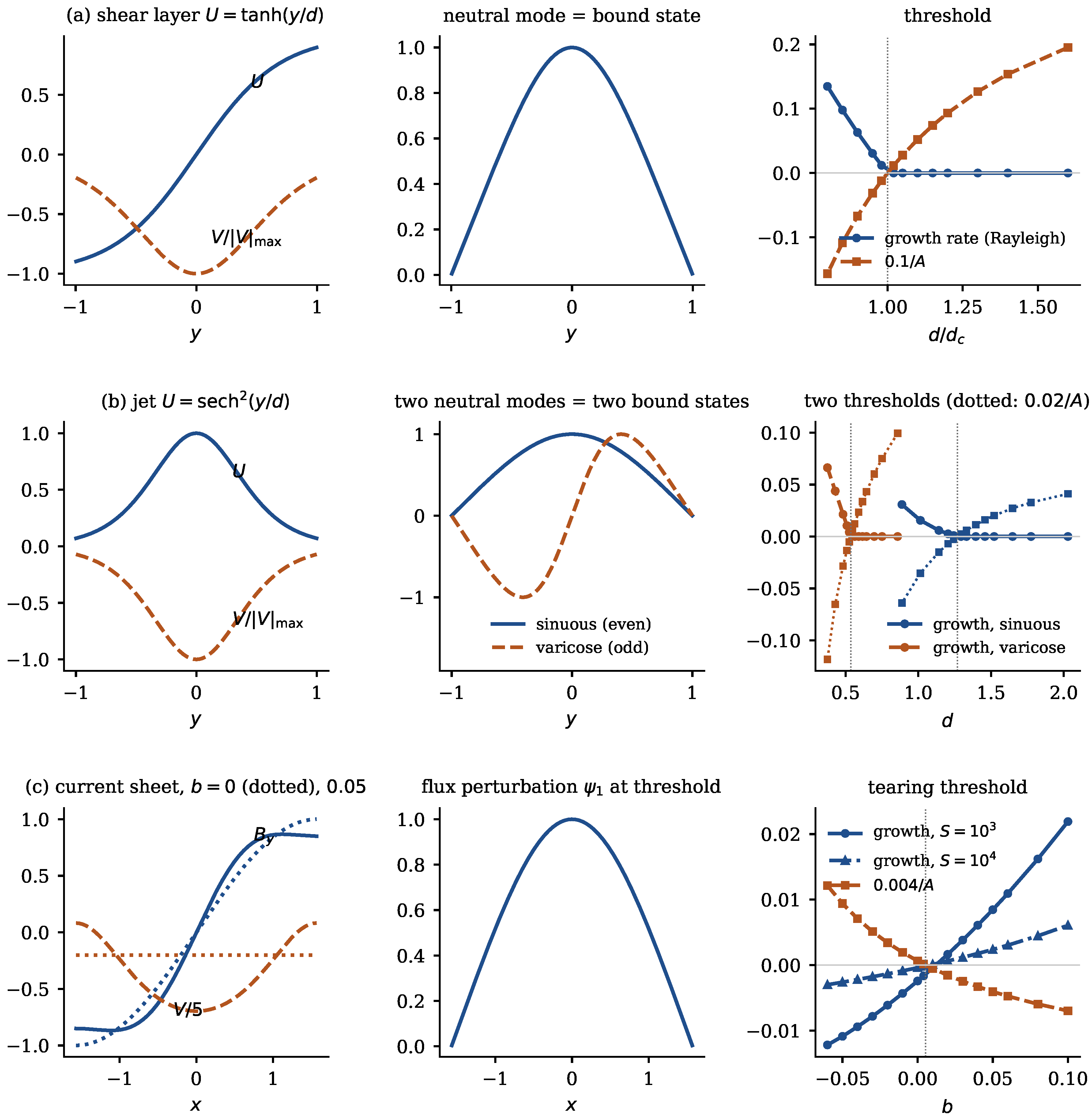
Figure 2.
Two shear layers at distance . (a) Velocity profiles. (b) The potential: a single well close to for small a, two wells for large a. (c) Neutral wavenumbers of the two bound states; the instabilities exist for .
Figure 2.
Two shear layers at distance . (a) Velocity profiles. (b) The potential: a single well close to for small a, two wells for large a. (c) Neutral wavenumbers of the two bound states; the instabilities exist for .
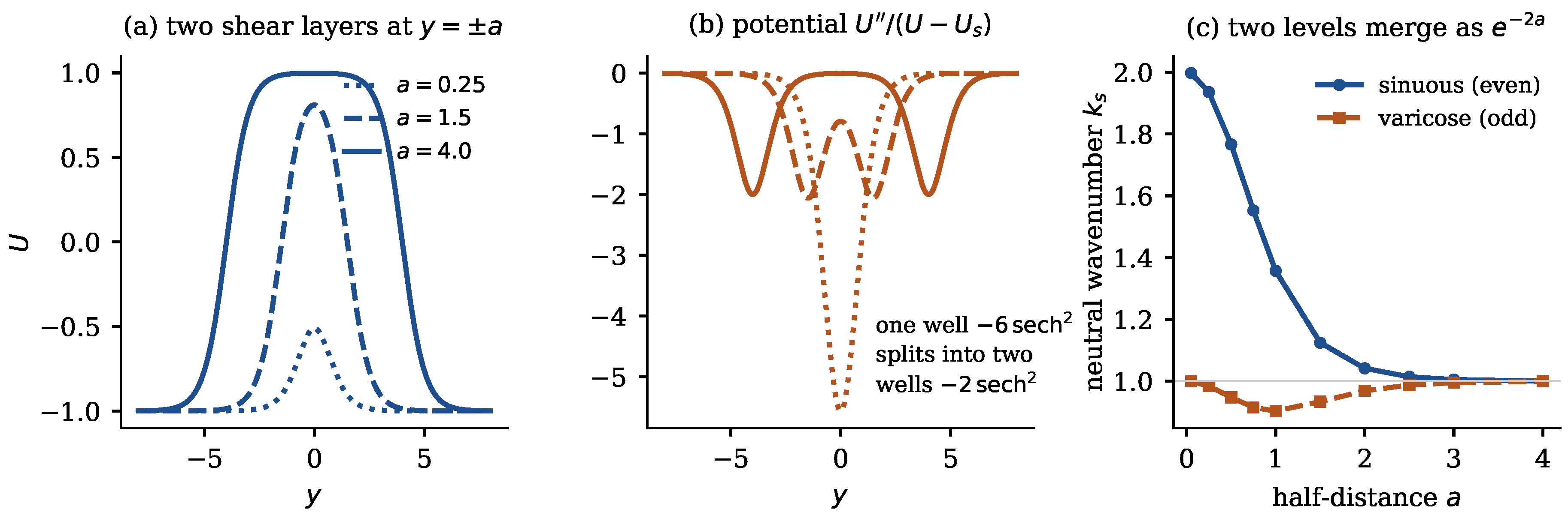
Figure 3.
The birth of a vortex from a shear layer between walls. (a) Vorticity for : the uniform layer, the growing wave, the roll-up, the closed core. (b) The final vortex for , where the layer has a bound state. (c) For , where it has none, the layer stays uniform. (d) Amplitude of the mode in both runs, with the inviscid Rayleigh growth rate. (e) Shape of the growing mode in the simulation, the Rayleigh eigenfunction and the bound state of .
Figure 3.
The birth of a vortex from a shear layer between walls. (a) Vorticity for : the uniform layer, the growing wave, the roll-up, the closed core. (b) The final vortex for , where the layer has a bound state. (c) For , where it has none, the layer stays uniform. (d) Amplitude of the mode in both runs, with the inviscid Rayleigh growth rate. (e) Shape of the growing mode in the simulation, the Rayleigh eigenfunction and the bound state of .
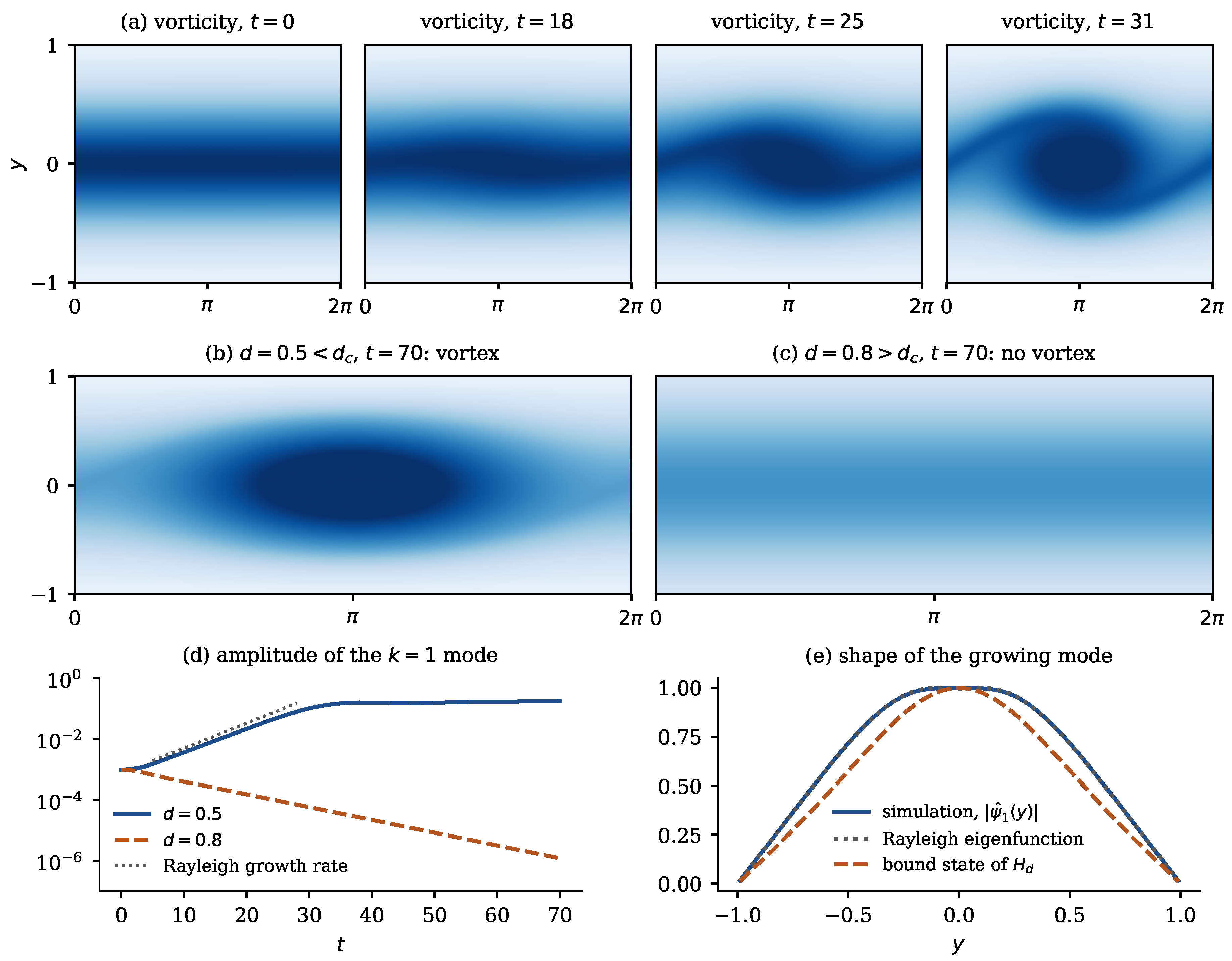
Figure 4.
Quantitative laws of the birth. (a) Growth rate against the binding energy of the bound state. (b) Amplitude of the final vortex against the distance from the viscous threshold , in logarithmic scales, with lines of slope and 1 for comparison. (c) Streamlines of the final vortex for ; thick curve: the separatrix; horizontal marks: the height predicted from the amplitude.
Figure 4.
Quantitative laws of the birth. (a) Growth rate against the binding energy of the bound state. (b) Amplitude of the final vortex against the distance from the viscous threshold , in logarithmic scales, with lines of slope and 1 for comparison. (c) Streamlines of the final vortex for ; thick curve: the separatrix; horizontal marks: the height predicted from the amplitude.
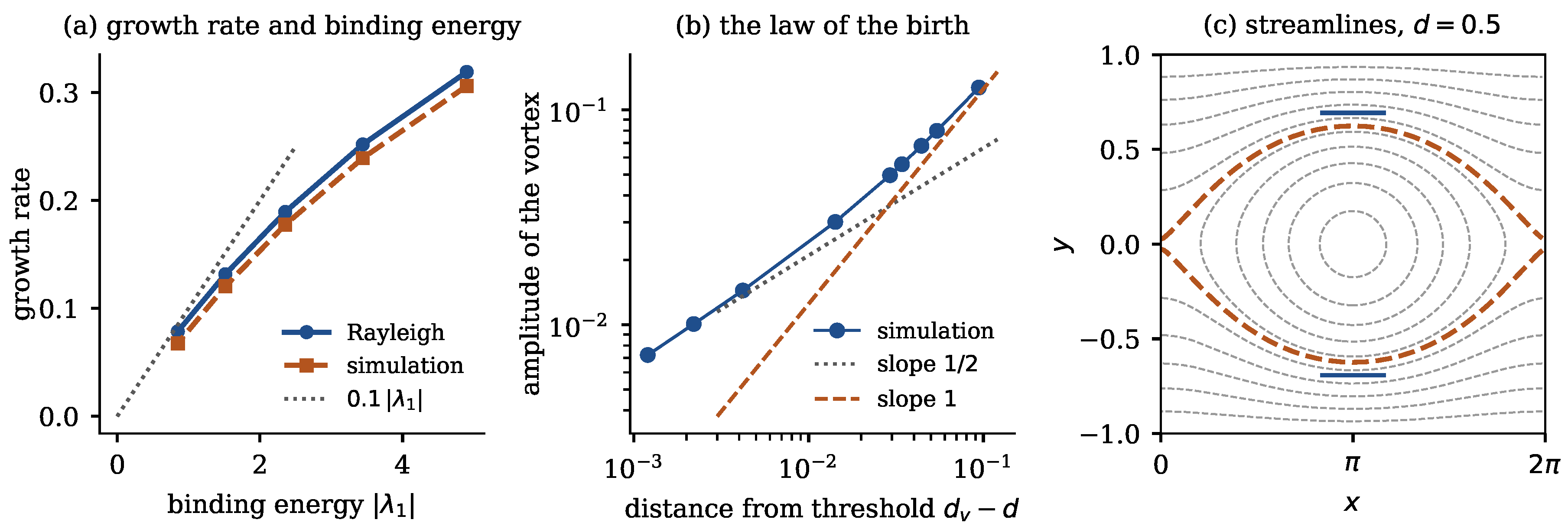
Figure 5.
Pressure in the birth of a vortex, incompressible flow. (a) Pressure (colour, from to ) and streamlines of the final vortex at . (b) Pressure along the critical level divided by ; thin line: . (c) The drop against the amplitude with the line , and the excess depth of the core with the line . (d) Pressure, vorticity and Reynolds stress across the layer through the core, each divided by its largest absolute value.
Figure 5.
Pressure in the birth of a vortex, incompressible flow. (a) Pressure (colour, from to ) and streamlines of the final vortex at . (b) Pressure along the critical level divided by ; thin line: . (c) The drop against the amplitude with the line , and the excess depth of the core with the line . (d) Pressure, vorticity and Reynolds stress across the layer through the core, each divided by its largest absolute value.
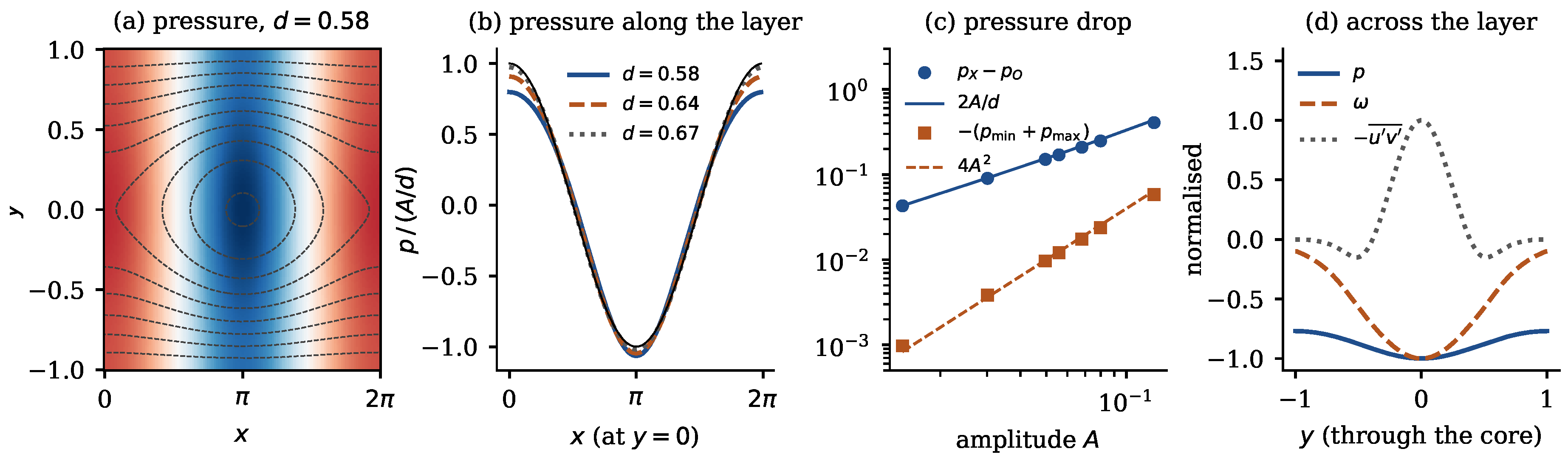
Figure 6.
Pressure in the birth of a vortex, compressible flow, . (a) at , ; the circle marks the steepest front. (b) Pressure across the steepest front, in cells along the normal. (c) Largest pressure gradient times the cell size against time. (d) Growth rate of the stationary mode against the Mach number; dotted line: , where the bound state of the unbounded layer leaves.
Figure 6.
Pressure in the birth of a vortex, compressible flow, . (a) at , ; the circle marks the steepest front. (b) Pressure across the steepest front, in cells along the normal. (c) Largest pressure gradient times the cell size against time. (d) Growth rate of the stationary mode against the Mach number; dotted line: , where the bound state of the unbounded layer leaves.
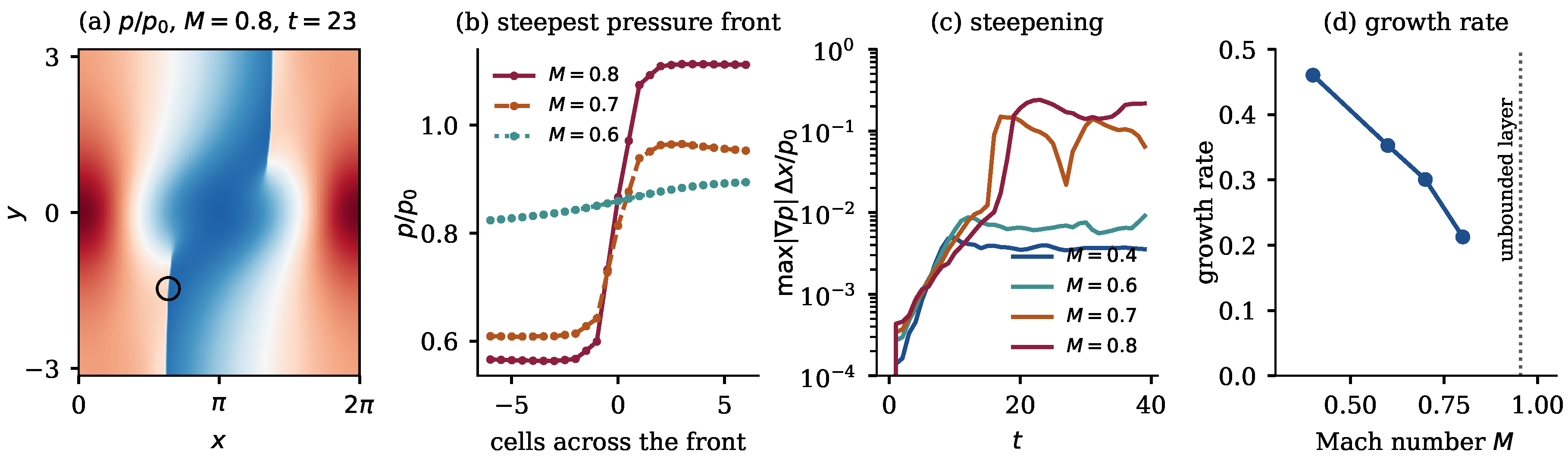
Figure 7.
Vortex instabilities as bound states. (a) Vorticity of shielded vortices. (b) The potential Q fixed by the vortex. (c) Growth rates of the modes from the Rayleigh problem; vertical dotted lines: birth of the bound state in the sector m. (d) Nonlinear evolution for : the instability forms a tripole. (e) For the instability forms a triangular core with three satellites. (f) Rayleigh discriminant of a swirl with tail . (g) Centrifugal growth rate against axial wavenumber; horizontal dotted lines: .
Figure 7.
Vortex instabilities as bound states. (a) Vorticity of shielded vortices. (b) The potential Q fixed by the vortex. (c) Growth rates of the modes from the Rayleigh problem; vertical dotted lines: birth of the bound state in the sector m. (d) Nonlinear evolution for : the instability forms a tripole. (e) For the instability forms a triangular core with three satellites. (f) Rayleigh discriminant of a swirl with tail . (g) Centrifugal growth rate against axial wavenumber; horizontal dotted lines: .
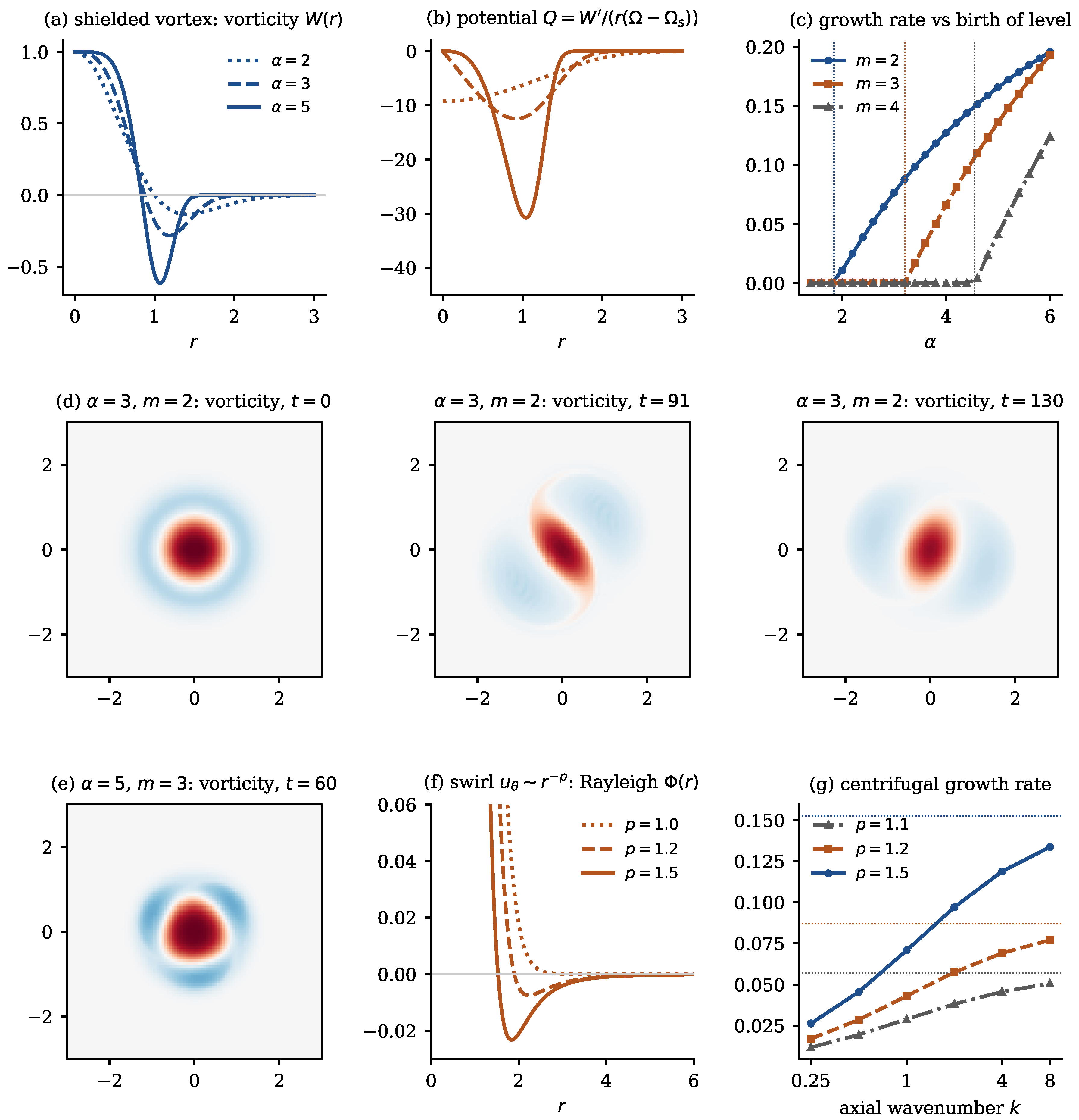
Figure 8.
Taylor vortices, . (a) Angular velocity, the potential and the radial velocity of the neutral mode across the gap. (b) The threshold , the lowest neutral eigenvalue of ; dot: , . (c) Taylor vortices at (two wavelengths shown): streamlines in the plane and the perturbation of the azimuthal velocity (colour, red: faster than the Couette flow). (d) Squared amplitude and excess torque against the Reynolds number; line: ; dotted: .
Figure 8.
Taylor vortices, . (a) Angular velocity, the potential and the radial velocity of the neutral mode across the gap. (b) The threshold , the lowest neutral eigenvalue of ; dot: , . (c) Taylor vortices at (two wavelengths shown): streamlines in the plane and the perturbation of the azimuthal velocity (colour, red: faster than the Couette flow). (d) Squared amplitude and excess torque against the Reynolds number; line: ; dotted: .
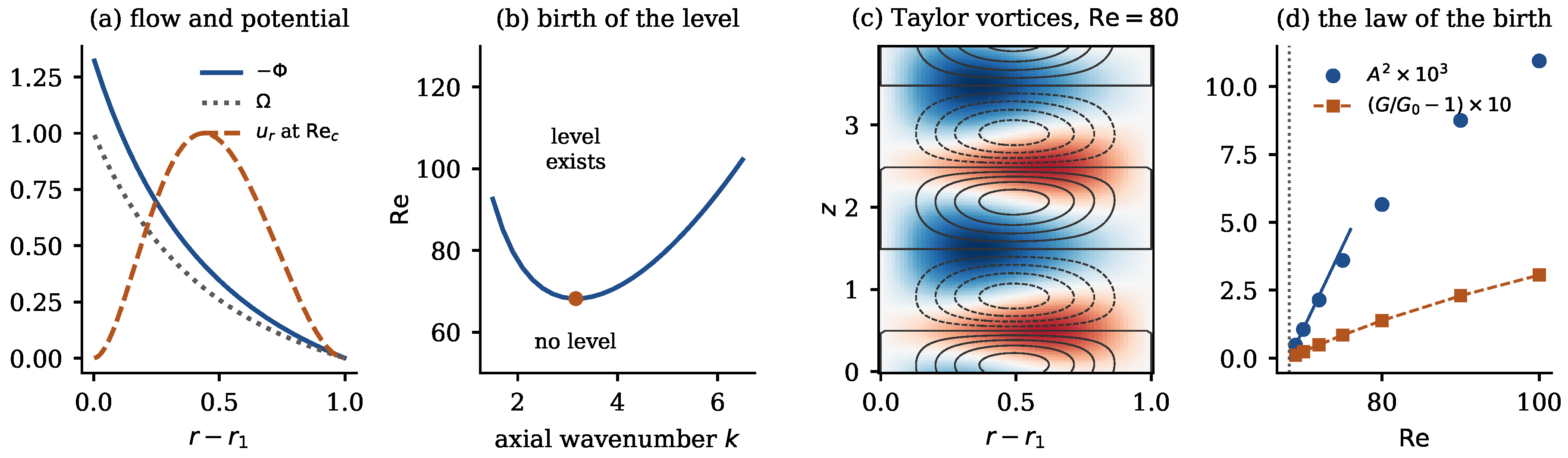
Figure 9.
Outflow from a nozzle. (a) Jet profile, the potential Q and the bound state for ; vertical line: . (b) Growth rate of axisymmetric modes for three thicknesses; triangles: the level . (c) Vorticity of the vortex rings at , two wavelengths. (d) Pressure at the same time (blue: low, in the cores).
Figure 9.
Outflow from a nozzle. (a) Jet profile, the potential Q and the bound state for ; vertical line: . (b) Growth rate of axisymmetric modes for three thicknesses; triangles: the level . (c) Vorticity of the vortex rings at , two wavelengths. (d) Pressure at the same time (blue: low, in the cores).
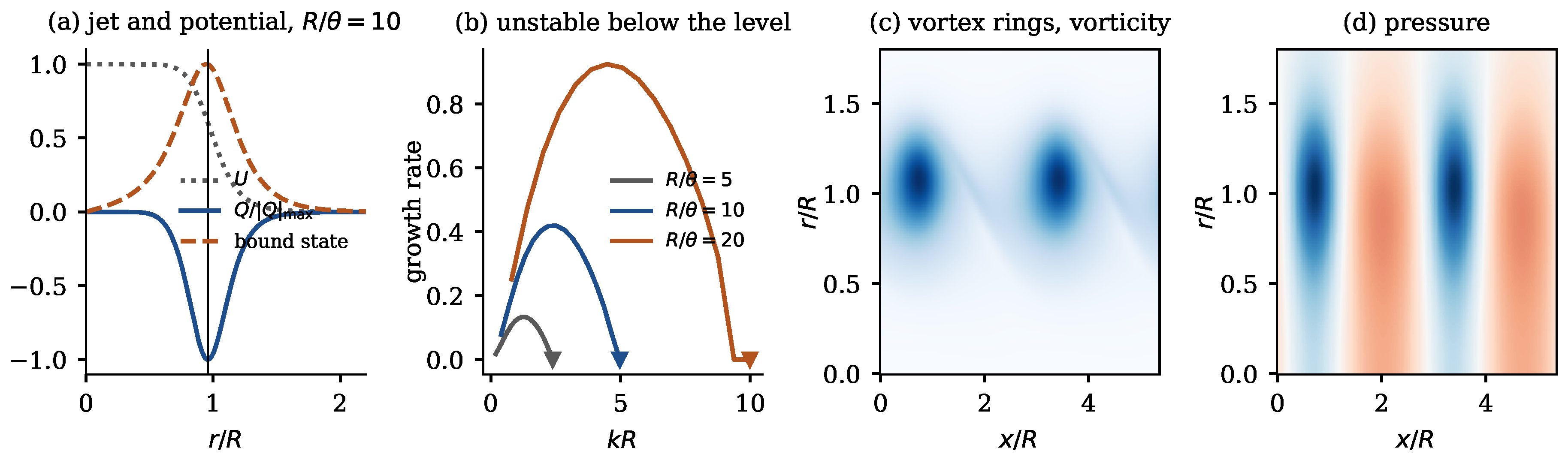
Figure 10.
(a) Growth rate of three-dimensional sinuous perturbations of the jet in the plane of wavevectors; the circles and are the two bound states of . (b) Rayleigh–Taylor growth rates for : formula (lines) and finite differences (dots). (c) Neutral curves of the stratified shear layer ; both touch Hardy’s constant .
Figure 10.
(a) Growth rate of three-dimensional sinuous perturbations of the jet in the plane of wavevectors; the circles and are the two bound states of . (b) Rayleigh–Taylor growth rates for : formula (lines) and finite differences (dots). (c) Neutral curves of the stratified shear layer ; both touch Hardy’s constant .
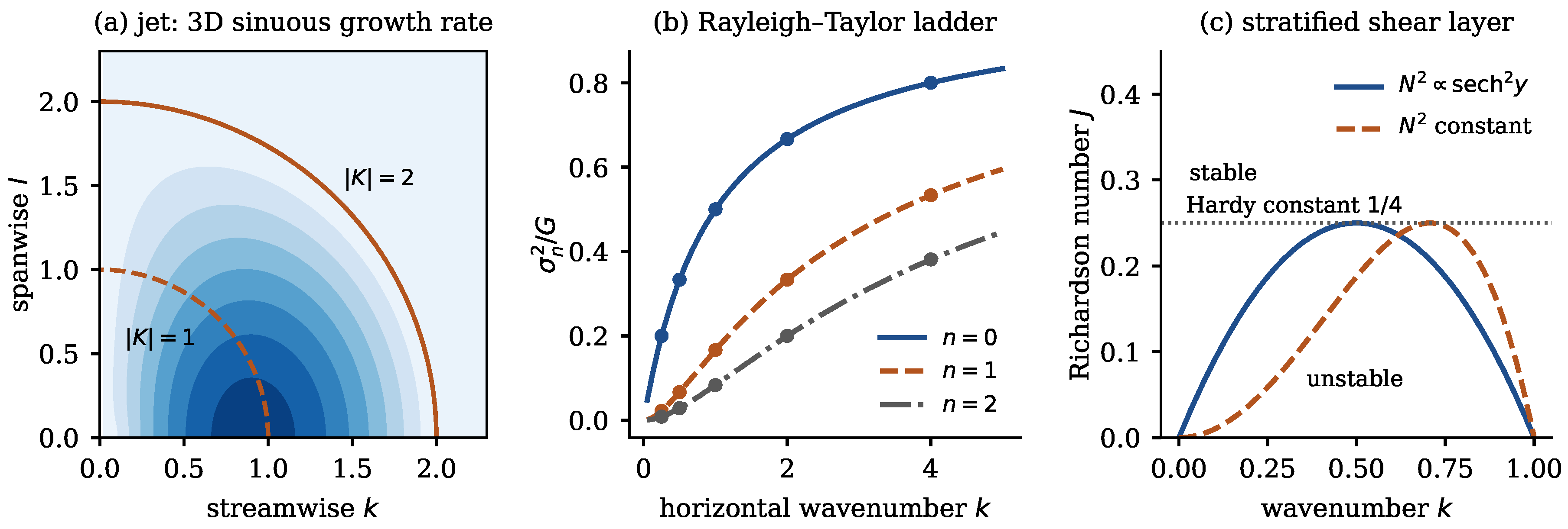
Figure 11.
(a) Densities of axisymmetric (, z-even) bound states of , , , in the half-plane: the ground state is one cell, higher states form a chain of cells along the axis, and the highest add a second radial row. (b) The inverse scattering length of the radial well passes through 0 at , where the zero-energy amplitude is infinite. (c) The bound state born at ; its energy follows near the threshold.
Figure 11.
(a) Densities of axisymmetric (, z-even) bound states of , , , in the half-plane: the ground state is one cell, higher states form a chain of cells along the axis, and the highest add a second radial row. (b) The inverse scattering length of the radial well passes through 0 at , where the zero-energy amplitude is infinite. (c) The bound state born at ; its energy follows near the threshold.
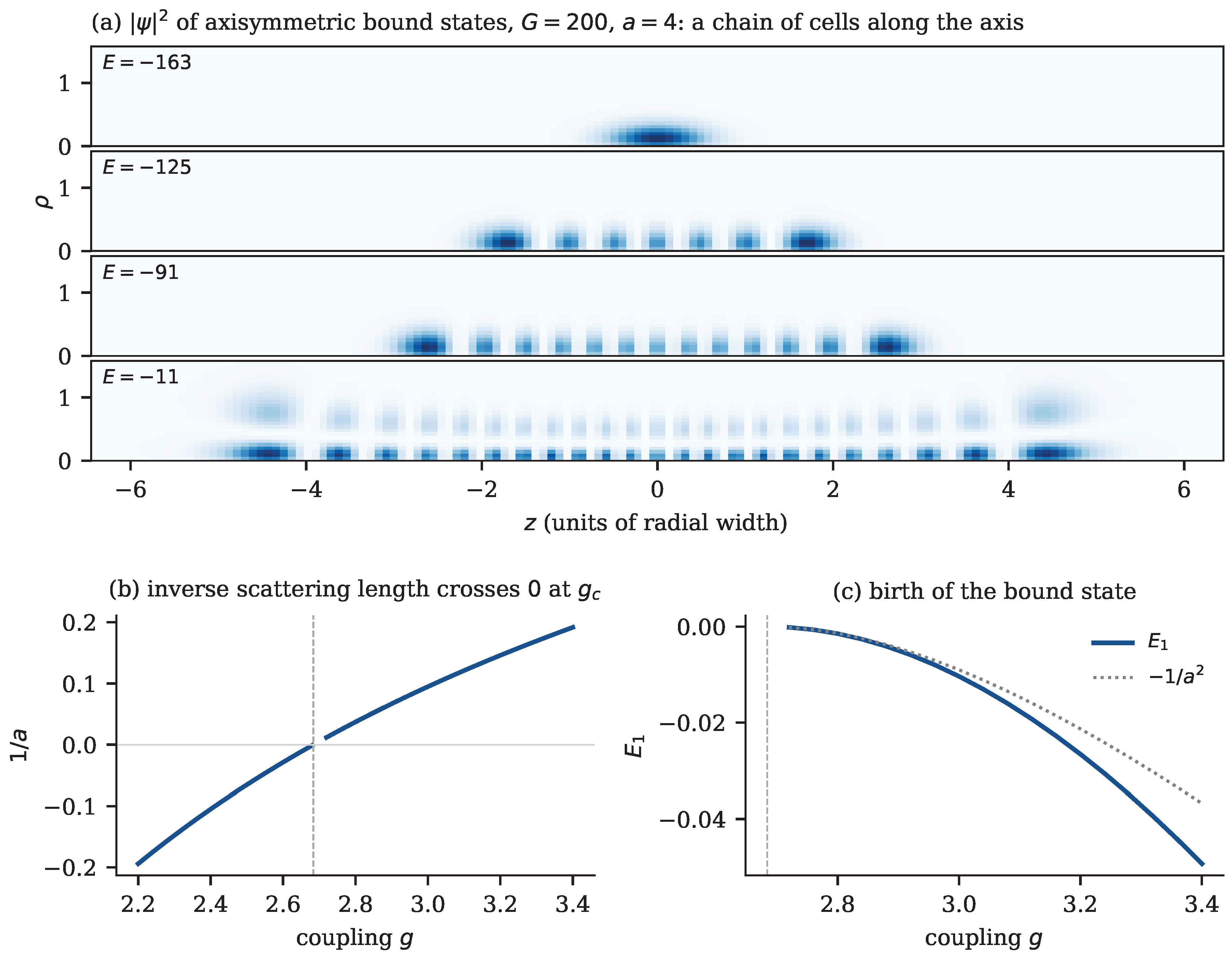

Table 1.
Error of the instability threshold predicted by linear extrapolation of from stable-side data.
Table 1.
Error of the instability threshold predicted by linear extrapolation of from stable-side data.
| data used, | inviscid | |||
|---|---|---|---|---|
Table 2.
Where the birth of a discrete state describes the onset of a new mode.
| Problem | Status of the bound-state picture |
|---|---|
| Free shear layers, jets, wakes | Exact (inviscid, for profiles with a bounded negative potential): Section 9, Section 13; viscous threshold checked for the layer. |
| Isolated vortices, tripoles | Exact (inviscid, two-dimensional): Section 11. |
| Centrifugal instabilities (Rayleigh, Taylor–Couette, Görtler) | Inviscid growth rate is a critical coupling (Section 11); for the Couette flow the viscous threshold is the lowest neutral eigenvalue of , checked with the nonlinear law of Taylor vortices (Section 11); Görtler vortices not computed. |
| Rayleigh–Taylor, thermal convection | Rayleigh–Taylor exact (this section); Rayleigh–Bénard onset is a sixth-order eigenvalue problem, classical. |
| Stratified shear (Kelvin–Helmholtz with stratification) | Richardson number is a Hardy coupling and is the critical constant, but the direction is reversed: the side with infinitely many levels is the stable one (this section). |
| Tearing modes, current sheets | Exact for the outer equation; resistive threshold close to it (Section 9). |
| Boundary layers, channel flow (Tollmien–Schlichting waves), hypersonic Mack modes | Travelling modes of non-self-adjoint operators; not computed here. |
| Pipe flow, plane Couette flow | Linearly stable at all Reynolds numbers; transition is subcritical, so no discrete mode is born. The picture does not apply. |
| Developed turbulence (spectra, intermittency, closure) | Not addressed. Only the count of Section 5 and its relation to degrees of freedom is relevant. |
Table 3.
First binding time of (“–”: no binding during the run) and time when first exceeds . Snapshot spacing: , , , .
Table 3.
First binding time of (“–”: no binding during the run) and time when first exceeds . Snapshot spacing: , , , .
| at | ||||||
|---|---|---|---|---|---|---|
| 2000 | 0.876 | – | – | – | 1.001 | 0.876 |
| 5000 | 0.314 | – | – | 0.391 | 0.314 | 0.314 |
| 10000 | 0.188 | – | 0.250 | 0.188 | 0.188 | 0.188 |
| 20000 | 0.094 | 0.422 | 0.141 | 0.141 | 0.141 | 0.094 |
Disclaimer/Publisher’s Note: The statements, opinions and data contained in all publications are solely those of the individual author(s) and contributor(s) and not of MDPI and/or the editor(s). MDPI and/or the editor(s) disclaim responsibility for any injury to people or property resulting from any ideas, methods, instructions or products referred to in the content. |
© 2026 by the authors. Licensee MDPI, Basel, Switzerland. This article is an open access article distributed under the terms and conditions of the Creative Commons Attribution (CC BY) license (http://creativecommons.org/licenses/by/4.0/).
Copyright: This open access article is published under a Creative Commons CC BY 4.0 license, which permit the free download, distribution, and reuse, provided that the author and preprint are cited in any reuse.