
Submitted:
06 November 2026
Posted:
09 November 2026
You are already at the latest version
Abstract
Reliable environmental perception is essential for intelligent ships, with three-dimensional (3D) point cloud ship detection providing spatial information for situational awareness and collision avoidance. However, unstable cross-frame geometric correspondence, ambiguous historical associations, and unreliable temporal fusion hinder the use of historical information. We propose GeoST for temporal maritime LiDAR ship detection, using object-local representations as a basis for geometric support-guided historical feature modulation and fusion. Built on FASTer, GeoST normalizes observations within their respective proposal coordinate systems and associates them by object dimensions and shape, constructing temporal inputs without external ego-vessel poses. The multi-scale anisotropic point feature enhancement module (PointMKDA) aggregates neighborhood features across scales and orientations to enhance local geometric representations. The geometrically constrained cross-attention module (GCAM) uses enhanced current-frame focal point features to update historical features and estimate geometric support. The reliability-guided feature modulation (RGFM) module combines this support, association priors, observation age, and learned features to generate modulation weights across temporal, point, and channel dimensions, regulating feature contributions before temporal fusion. GeoST achieved 3D average precision (AP) of 87.17% and 73.09% at intersection-over-union (IoU) thresholds of 0.5 and 0.7, respectively, exceeding FASTer by 2.81 and 2.27 percentage points.
Keywords:
maritime ship detection
; LiDAR point clouds
; object-local representations
; geometric support
; temporal fusion
; feature modulation
1. Introduction
Environmental perception is essential for autonomous maritime navigation, providing information about surrounding vessels and obstacles for navigation planning and collision avoidance [1,2]. Ship detection is a key part of this process, as estimates of vessel positions, dimensions, and orientations provide geometric inputs for target tracking and collision-risk assessment. The quality of perception measurements also affects the reliability of subsequent collision-avoidance decisions [3]. LiDAR directly measures the three-dimensional structure of the surrounding environment, making it suitable for the spatial localization and geometric characterization of vessel targets [4,5]. Accurate ship detection from LiDAR point clouds is therefore important for maritime situational awareness.
Despite these advantages, accurate ship detection from maritime LiDAR point clouds remains challenging. Point density varies considerably with observation distance, leaving distant vessels sparsely represented. Changes in viewing direction and partial occlusion further complicate maritime target perception [6]. The resulting point clouds may cover only part of the hull and superstructure, leaving the vessel’s full spatial extent insufficiently observed. Differences in vessel size and shape also introduce substantial variation in the geometric structures that a detector must represent [7]. Together, these factors complicate the estimation of bounding-box positions, dimensions, and orientations from incomplete returns. For elongated vessels, orientation errors can additionally produce pronounced boundary deviations at the hull ends. Recent work has incorporated LiDAR intensity to enhance maritime object representations, providing one approach to extracting additional information from the available observations [8].
Temporal observations provide an opportunity to supplement the incomplete geometric evidence available for ship detection. As the relative viewing geometry changes, historical scans may retain vessel structures that are poorly represented in the current observation. Existing temporal detectors exploit sequential information through multi-frame feature interaction [9], motion-guided fusion [10], and point–trajectory modeling [11]. Effective use of these observations nevertheless depends on both cross-frame comparability and the relevance of the retrieved historical evidence.
This study considers a LiDAR-based refinement setting in which external ego-vessel poses are not used for cross-frame alignment. Expressing observations in their respective proposal-local coordinate systems reduces dependence on absolute position and heading, but does not establish exact geometric correspondence. Proposal errors and changes in visible surfaces can introduce local inconsistencies, while vessels with similar dimensions and partial shapes may create association ambiguity. Historical observations also differ in age and in the structural information they provide. Consequently, effective temporal refinement must distinguish locally compatible evidence from observations that offer limited support for the current target, rather than treating all associated history as equally useful.
To address these issues, we propose GeoST, a temporal refinement framework for maritime ship detection in LiDAR point clouds. GeoST retains the focal point selection and grouped hierarchical fusion (GHF) of FASTer [12]. Historical inputs are constructed by normalizing each observation in its own proposal coordinate system and associating observations based on object dimensions and shape, without external ego-vessel poses. Within this framework, current-frame geometry guides both historical feature updates and their subsequent use in temporal fusion. The multi-scale anisotropic point feature enhancement module (PointMKDA) strengthens current features before focal-point selection. The geometrically constrained cross-attention module (GCAM) uses the selected current features to update historical features within local geometric neighborhoods and estimate geometric support. This support is passed to the reliability-guided feature modulation (RGFM) module, where it is combined with association priors, observation age, and learned features to regulate feature contributions before temporal fusion. When no valid historical support is available, the current-frame prediction is used.
The main contributions of this study are as follows:
- A framework for temporal ship detection is developed to use maritime LiDAR sequences without external ego-vessel pose inputs. The framework represents observations in their respective proposal-local coordinate systems and constructs historical inputs through association based on object dimensions and shape.
- A refinement mechanism is introduced in which geometric support estimated during cross-frame interaction guides feature modulation before temporal fusion. PointMKDA strengthens the current geometric reference, GCAM uses this reference to update historical features and estimate geometric support, and RGFM combines the resulting support with association priors and observation age to regulate feature contributions. This connection allows the local compatibility assessed during cross-frame interaction to directly influence the subsequent use of historical information.
- GeoST is evaluated on real maritime LiDAR sequences using 3D average precision (AP). At intersection-over-union (IoU) thresholds of 0.5 and 0.7, it achieves AP values of 87.17% and 73.09%, respectively. These values exceed those of FASTer by 2.81 and 2.27 percentage points, respectively. Controlled comparisons of historical-input configurations and module ablations further examine the contributions of temporal information and the proposed refinement components.
The remainder of this paper is organized as follows. Section 2 reviews related work on point-cloud-based three-dimensional detection and temporal detection. Section 3 presents the proposed framework. Section 4 presents the experimental setup, analyzes the contribution of historical information and the effect of history window size, and reports module ablations, performance comparisons, and qualitative evaluations. Section 5 discusses the findings and limitations. Section 6 concludes the paper.
2. Related Work
2.1. Point-Cloud-Based Three-Dimensional Object Detection
Point-cloud detectors employ different spatial representations to balance geometric detail and computational cost. PointPillars [13] organizes points into vertical columns for efficient feature extraction. More recent architectures exploit sparse voxel representations. VoxelNeXt [14] performs fully sparse detection, DSVT [15] models voxel relationships through attention over dynamically partitioned sets, and SAFDNet [16] introduces adaptive feature diffusion to address missing features near object centers. LargeKernel3D [17] expands spatial receptive fields through large-kernel sparse convolutions, while HEDNet [18] uses hierarchical encoder–decoder blocks to capture relationships among spatially disconnected features. These approaches further emphasize the importance of spatial context for sparse point-cloud detection.
Point-level representation learning provides complementary approaches to geometric feature extraction. PointNeXt [19] revisits hierarchical point processing through improved training and scalable architectures. Point Transformer V2 [20] introduces grouped vector attention and partition-based pooling, while Point Transformer V3 [21] uses serialized neighborhood mapping to support efficient feature interaction over larger receptive fields. These studies motivate the investigation of neighborhood aggregation for representing local ship structures.
Proposal-based methods further exploit regional geometry to refine coarse predictions. PointRCNN [22] learns local features in proposal-relative canonical coordinates, while PV-RCNN [23] and PV-RCNN++ [24] combine voxel encoding with point-based feature aggregation. CT3D [25] introduces proposal-aware embedding and channel-wise Transformer decoding, and CT3D++ [26] further integrates geometric and semantic information through bidirectional encoding. These studies establish the importance of object-local evidence for bounding-box refinement.
2.2. Temporal Three-Dimensional Object Detection
Temporal detectors incorporate sequential observations through feature aggregation and cross-frame alignment. 3D-MAN [27] employs multi-frame attention, while CenterFormer [28] supports temporal feature fusion within a center-based Transformer detector. MGTANet [29] combines short-term motion-aware encoding with long-term feature enhancement. D-Align [30] uses dual-query co-attention and gated aggregation to integrate sequential bird’s-eye-view features. More recently, MAD [31] extends temporal reasoning through an object memory bank, using trajectory forecasts and ego poses to align historical proposals. DetZero [32] explores long-sequence refinement in an offboard setting.
Region-based temporal refinement also seeks to retain object-level geometric detail while controlling the cost of historical processing. FASTer [12] introduces adaptive focal-token selection and GHF for efficient long-sequence detection. Its single-frame stage selects informative points for storage, while its multi-frame stage progressively aggregates the retained historical observations. Historical inputs are organized through box trajectories and encoded using their geometric relationships to the current proposal. This design provides an efficient backbone for long-sequence refinement.
These studies address temporal detection through different forms of alignment, feature aggregation, and memory organization. The present work considers historical observations represented in their respective proposal-local coordinates without external ego-vessel poses. Under this representation, association does not guarantee local geometric correspondence, and historical observations may provide different levels of support for the current target. GeoST therefore uses geometrically constrained cross-attention to update historical features and estimate geometric support, which guides feature modulation before temporal fusion.
3. Methodology
3.1. Overall Framework and ROI-Local History Construction
Figure 1 presents GeoST, which refines current-frame ship proposals using object-local representations and geometric support-guided temporal fusion. Given initial proposals generated by CenterPoint [33], PointMKDA enhances current region of interest (ROI) features before the single-frame sequence processing (SSP) module selects focal points. Historical observations are associated with current proposals and represented in their respective ROI coordinates. GCAM updates historical features through geometrically constrained interaction with the current focal points and estimates their geometric support. RGFM combines this support with association priors and observation age to generate modulation weights across temporal, point, and channel dimensions. These weights regulate feature contributions before grouped temporal fusion in the multi-frame sequence processing (MSP) module. The fused representation produces refined detections, while SSP provides the prediction when historical support is unavailable. The SSP and MSP stages adopt the refinement backbone of FASTer [12].
To construct temporal inputs without external ego-vessel poses, each observation is normalized using its own predicted box. For a proposal with center , dimensions , and yaw angle , an ROI point is transformed as
where denotes normalized local coordinates, rotates the point into the proposal’s horizontal axes, and scales the coordinates by the box half-dimensions. This establishes a common coordinate convention across observations, although exact alignment is not guaranteed.
Historical inputs are constructed from a fixed window of the most recent earlier records within the same sequence and dataset split, subject to a maximum time difference of 8 s. No additional temporal subsampling is applied during window construction, and observation ages are calculated from the recorded timestamps. For shape association, proposal crops are enlarged by a factor of 1.2, and their local coordinates are normalized by the full box dimensions, giving . Up to 512 points are selected using deterministic farthest point sampling; proposals containing fewer than six points are excluded from association.
Each shape descriptor comprises a normalized occupancy histogram over and a 20-dimensional vector containing the 10th, 25th, 50th, 75th, and 90th percentiles of each coordinate of and the radial distance . The shape distance and association cost are defined as
where is the mean absolute logarithmic ratio of corresponding box dimensions. Candidate pairs must have matching predicted classes, confidence scores of at least 0.1, a maximum absolute logarithmic dimension ratio no greater than 0.7, and . Historical candidates must also have valid cached SSP-selected points. Only mutual minimum-cost matches are retained. In each matching direction, the gap between the best and second-best finite costs must be at least 0.05 whenever a second candidate exists. For an accepted match between current proposal i and historical proposal j, the historical prior is defined as , where k indexes the historical slot, is the historical detection score, and is the shape-distance threshold.
Historical points are retrieved through cached SSP selection indices and encoded using local geometry, intensity, observation age, and predicted dimensions. Together with the selected current-frame points, they form the temporal input to GCAM, which provides updated features and geometric support for RGFM. Failed associations and missing observations remain masked without duplication or replacement by older frames. Cached indices are updated only after the current forward pass.
3.2. Multi-Scale Anisotropic Point Feature Enhancement
Sparse ship point clouds often provide uneven coverage of elongated hulls and vertical structures. To capture these geometric characteristics, PointMKDA enhances current ROI features using neighborhoods with different scales and orientations, as illustrated in Figure 2. The enhanced features are then passed to SSP for focal-point selection, providing the current reference for subsequent cross-frame interaction.
For each point n, the initial feature encodes offsets relative to the ROI corners and center, together with intensity and a zero age value. It is then concatenated with the normalized coordinates and mapped to an embedding through a linear projection, layer normalization (LN), and a Gaussian error linear unit (GELU) activation. The nine ellipsoidal branches use semiaxes , , and , where . Valid neighbors within each ellipsoid are ranked by ellipsoidal distance, with a nominal budget of 12 points including the query point; ties at the cutoff are retained. Neighborhoods containing fewer points use all available valid points without duplication.
For branch b, the normalized offset, aggregation weight, and branch feature are defined as
where contains the ellipsoid semiaxes and is the corresponding diagonal scaling matrix. The set contains the selected valid neighbors of point n in branch b, satisfying . The geometric descriptor concatenates the weighted mean offsets and weighted mean absolute offsets. A shared multilayer perceptron (MLP) encodes this descriptor, while the learned projection maps neighboring features. Each branch therefore combines feature evidence with local spatial structure.
For each point, branch weights are predicted from its embedding, and the weighted branch features are incorporated through a residual update:
where is the weight of branch b, , , and are learned projections, is a bias, and is a learnable residual scale initialized to 0.1. The softmax operates over valid branches, and invalid points are masked throughout processing. This adaptive combination incorporates neighborhood evidence at different scales and orientations while preserving point coordinates and counts.
The enhanced features are processed by the retained SSP module to produce focal points and an object token. All 57 current focal points serve as references for GCAM, while the first 48 selected raw-point slots form the current temporal input. The object token supports current-frame prediction and subsequently queries the temporally fused features.
3.3. Geometrically Constrained Cross-Attention
Although ROI normalization provides a common coordinate convention, proposal errors and changes in visible surfaces can still produce discrepancies between observations. Independently sampled historical points also lack explicit correspondence with current focal points. GCAM therefore restricts cross-frame interaction to local geometric neighborhoods and estimates support for subsequent feature modulation, as illustrated in Figure 3.
Historical features provide queries, while current focal features provide keys and values. The two streams undergo separate layer normalization followed by learned projections. For historical point n in slot k, the eligible reference set contains valid current focal points within distance r in normalized ROI coordinates. GCAM uses four attention heads, with the distance threshold set to in these normalized coordinates. Historical slots are eligible only when their association priors are positive and finite and their observation ages are finite.
For attention head h, the interaction weights are
where and are the projected query and key, is the head dimension, and is the distance between the historical point and current reference q. The nonnegative learnable coefficient controls the distance penalty. The neighborhood threshold excludes distant references, while the penalty adjusts their relative contributions within the eligible region. Empty reference sets produce zero attention and zero aggregated evidence.
Historical features are updated by aggregating value vectors from the current reference points:
where is the encoded historical feature, is the projected current value, is the output projection, and is a learnable residual scale initialized to 0.1. Historical points without eligible references receive zero aggregated evidence and retain their input features. Invalid points are masked, and the current temporal slot bypasses this update.
The same attention weights are used to estimate geometric support:
where denotes attention averaged across heads, is the observation age, and is a nonnegative learnable decay coefficient. The coefficients and are parameterized using softplus, with their underlying parameters initialized to zero, yielding an initial value of for each coefficient. Points without eligible references receive zero support, while valid current-slot points receive unit support.
The support value summarizes local distance consistency and observation age rather than a correspondence probability. GCAM passes both the updated features and geometric support to RGFM, where they are used together with association priors and observation age to generate modulation weights for subsequent temporal fusion.
3.4. Reliability-Guided Feature Modulation and Prediction
Historical observations differ in association quality, observation age, and geometric support. RGFM combines these cues with learned features to generate modulation weights across temporal, point, and channel dimensions, as illustrated in Figure 4. It first performs channel-wise competition across temporal slots and then combines pointwise gating with local geometric support to regulate feature contributions before grouped temporal fusion in MSP.
Let denote the layer-normalized GCAM output for point n in slot k. The slot descriptor and mean support are computed over valid points. Valid points with zero support remain in the averaging denominator, so the mean support reflects both support strength and the fraction of supported points. Association priors and support values are clipped to . A slot is eligible for temporal competition when its association prior is positive and at least one valid point has positive support.
The channel-wise competition logits and weights are
where is the association prior, is the observation age, and c indexes feature channels. The MLPs and encode the slot feature and conditioning cues, respectively. Numerical stability is ensured by . The nonnegative age-decay coefficient is parameterized as , where is a learnable scalar initialized to zero.
A pointwise gate further regulates individual feature contributions:
where is a pointwise MLP, is the validity mask, and is the support supplied by GCAM. The current slot participates with unit association prior, zero age, and unit support at valid points. Historical contributions are additionally attenuated by their pointwise support. Gates are computed independently within each slot, without requiring correspondence between equal point indices across frames.
MSP receives the GCAM output features, while the normalized features are used to generate modulation weights in RGFM. Points with no positive channel weight are masked before the first SpatialDrop block. After this block completes point selection, attention, and feed-forward processing with their residual and normalization operations, the modulation weights are gathered using the same selection indices and applied once to the corresponding output features before grouped temporal fusion. This placement preserves the feature modulation after the block’s normalization stages. The remaining MSP hierarchy aggregates the temporal features, which are queried by the current SSP object token to predict a foreground logit and seven box residuals.
The temporal prediction is selected when any historical weight is positive before SpatialDrop sampling. Otherwise, both classification and regression use the SSP prediction. This selection depends on the availability of historical support rather than a calibrated confidence threshold. Box residuals are decoded relative to the current proposal, whose predicted class is retained.
3.5. Training Objective and Procedure
The initial detection proposals remain fixed during training, and only the refinement network is optimized. The objective combines classification, box regression, SSP auxiliary supervision, and corner consistency without requiring correspondence or reliability labels.
Each proposal is assigned to the same-class ground-truth box with the highest oriented 3D IoU, measured before refinement. The IoU is set to zero when no same-class ground truth exists. Classification uses the soft target , while box regression is applied only to proposals with IoU greater than 0.55.
The seven regression targets describe center offsets, dimension ratios, and heading difference relative to the current proposal. Center offsets are rotated into the proposal axes, with horizontal components normalized by and the vertical component by h. Dimension targets use logarithmic ratios, and the heading target is wrapped to . Regression compares predicted and target residuals directly.
The total training loss is
where is binary cross-entropy with logits, averaged over the final prediction and the three SSP outputs. The final box regression loss uses Smooth L1 with transition parameter and equal weights for all seven components. The auxiliary loss averages the regression losses of the three SSP outputs, whose prediction heads share parameters.
The corner loss supervises the selected final box. For each predicted corner, distances are computed to the corresponding corners of the ground-truth box and a version of that box rotated by . The smaller distance is penalized using Smooth loss with a transition parameter of 1. This term is averaged over the eight corners and eligible proposals. Regression losses are normalized by the number of eligible proposals and vanish when none are available.
SSP auxiliary supervision remains active when the final prediction uses the current-frame fallback. Training proceeds chronologically within each sequence, with one optimizer update per frame containing valid proposal point observations and a constant learning rate. The historical cache is reset at sequence boundaries and at the start of each training or validation epoch. Historical inputs are constructed only from earlier frames, and ground truth is used solely for supervision.
4. Experiments and Analysis
4.1. Experimental Setup
A custom maritime ship LiDAR point cloud dataset was constructed using data collected aboard the Dolphin-1 intelligent vessel platform, which was designed by Harbin Engineering University. Field trials were conducted in offshore waters, where an onboard RoboSense RS-Ruby 128-beam LiDAR continuously recorded raw point cloud sequences at 10 Hz. The data collection vessel operated in coordination with two target speedboats. Their relative positions, headings, and speeds were varied to capture ship point clouds during overtaking, head-on encounters, crossing encounters, and circling maneuvers. Each frame contained 3D point coordinates and return intensities, together with a sequence identifier and timestamp. Ships were treated as a single detection class and annotated with 3D bounding boxes specifying their center positions, dimensions, and heading angles in the LiDAR coordinate system. The dataset comprised 10,547 point cloud frames and was partitioned by complete acquisition sequence into training, validation, and test sets at an approximate ratio of 8:1:1. Fixed, non-overlapping sequence lists were used to ensure consistent partitioning.
Model training was performed on a computing platform equipped with an NVIDIA GeForce RTX 4090 GPU with 24 GB of memory. The software environment comprised Ubuntu 22.04, Python 3.10, PyTorch 2.0.1, CUDA 11.8, and spconv 2.3.6. All baseline detectors were trained using their respective original training configurations. For GeoST, training consisted of two stages: proposal detection and temporal refinement. First, a single-frame CenterPoint front end was trained to generate proposals and their confidence scores. The front-end checkpoint and generated proposals were then fixed while the back-end refinement model was trained. The refinement stage used the AdamW optimizer with an initial learning rate of 0.001 and a weight decay of 0.01. The model was trained for 30 epochs with a gradient norm clipping threshold of 10 and a random seed of 42. Training samples were processed in chronological order within each sequence, and model checkpoints were selected based on validation loss. The number of refinement feature channels was set to 256. Point budgets were set to 192 for the current proposal region and 48 per temporal slot. FASTer used externally provided ego-vessel poses for temporal processing. GeoST constructed temporal inputs without external ego-vessel poses during either training or evaluation. The total number of input frames used by each method, including the current frame, is reported in Table 4.
Detection performance was evaluated using 3D AP at 3D IoU thresholds of 0.5 and 0.7. The corresponding AP metrics are denoted by AP@0.5 and AP@0.7, respectively. During evaluation, predicted boxes were ranked by confidence and matched one-to-one with previously unmatched ground-truth boxes in the same frame. Matches satisfying the IoU threshold were counted as true positives, whereas duplicate detections and unmatched predictions were counted as false positives. AP was computed using 101-point interpolation by averaging interpolated precision at uniformly spaced recall levels over [0, 1], with zero precision assigned to recall levels that were not reached. To examine performance at different observation ranges, targets were divided into two groups according to the distance from the target center to the LiDAR sensor: L1 for distances below 60 m and L2 for distances of at least 60 m. Overall AP and range-specific AP were calculated separately from their respective precision–recall curves, and differences in AP were reported in percentage points. All methods used the same data split, test frames, metric computation procedure, and rules for range grouping, matching, and ignoring instances. For post-processing, the proposed model used a confidence threshold of 0.1 and a 3D non-maximum suppression IoU threshold of 0.1.
4.2. Analysis of Historical Information Utilization
4.2.1. Contribution of Historical Information
Three controlled configurations of GeoST were established to examine the effects of historical information during training and evaluation, as summarized in Table 1. In S0, historical input was disabled during both training and evaluation, and detections were produced by the SSP branch. In S1, historical input was enabled during training but disabled during evaluation, with detections likewise produced by SSP. In S2, historical input was enabled during both stages, allowing historical observations to refine the current-frame 3D bounding boxes through cross-frame feature interaction and temporal fusion. S1 and S2 were evaluated using the same trained checkpoint, differing only in historical-input availability and the corresponding prediction pathway during evaluation. The comparison between S0 and S1 assessed how the use of historical information during training affected current-frame detections. The comparison between S1 and S2 further examined the performance changes associated with enabling historical input and the corresponding temporal output path during evaluation. Figure 5 presents the detection performance and corresponding gains for each configuration. Here, pp denotes percentage points, representing the absolute difference between AP values expressed as percentages.
Enabling historical input and the corresponding temporal output path during evaluation further increased the AP@0.5 and AP@0.7 of S2 to 87.17% and 73.09%, respectively, representing gains of 3.08 and 3.13 percentage points over S1. As shown in Figure 5, both gains were substantially larger than those of S1 over S0, suggesting that the use of historical observations during evaluation contributed more to the observed improvement. During evaluation, S1 made predictions from the current frame, whereas S2 incorporated historical observations into feature fusion and 3D box refinement through the temporal path, allowing cross-frame information to contribute directly to the resulting detections.
Relative to S0, S2 achieved cumulative gains of 3.49 and 3.67 percentage points in AP@0.5 and AP@0.7, respectively, with both metrics increasing successively from S0 to S1 to S2. The gains of S2 over S1 were similar at the two thresholds, indicating that temporal information remains beneficial under stricter 3D box matching requirements. This observation is consistent with the proposed design, which supports temporal fusion through local geometric feature enhancement, geometrically constrained cross-frame interaction, and modulation of historical contributions. Together, the three configurations show that using historical information during training improves current-frame detection, while incorporating historical observations into temporal inference during evaluation yields further benefits for 3D ship detection.
4.2.2. Sensitivity to History Window Size
To examine the influence of history window size on ship detection performance, the maximum number of historical frames was set to . A separate model was trained for each window configuration and evaluated on the validation set using the corresponding historical input limit. All configurations followed the same processing pipeline. Here, H excludes the current frame, so the maximum total number of observed frames is . The H = 0 configuration corresponded to an independently trained model that used no historical information during either training or evaluation. The results and their trends are presented in Table 2 and Figure 6, respectively. Figure 1 and Figure 4 illustrate the default configuration with , where 16 temporal slots are first fused into four groups and then into a single group. For , the input includes the current frame and up to 20 historical frames, with the 21 temporal slots first fused into seven groups and then into a single group.
Short history windows provided substantial initial gains. At , AP@0.5 and AP@0.7 reached 85.14% and 70.66%, respectively, exceeding by 1.22 and 1.35 percentage points. At , the corresponding gains increased to 2.13 and 2.42 percentage points. Different viewpoints and return distributions provide complementary observations of local hull structures, allowing historical information to supplement regions that are missing or sparsely represented in the current frame. This structural complementarity helps explain why substantial improvements were obtained with relatively short windows.
The incremental benefits diminished as the window expanded. Increasing H from 3 to 7 improved the two metrics by 0.71 and 0.69 percentage points, whereas increasing H from 7 to 15 yielded smaller gains of 0.32 and 0.34 percentage points. Additional observations often contain hull structures already represented in the available history, so increasing the frame count does not necessarily provide a proportional increase in independent geometric information. The diminishing gains are consistent with this overlap, while the remaining benefit also depends on the compatibility of newly included observations with the current target structure.
Both metrics peaked at , reaching 87.08% and 72.76%. At , they decreased by 0.45 and 0.52 percentage points, respectively, and fell below the results. Extending the window can introduce observations with different visible surfaces and less compatible proposal geometry, increasing the demands on association and temporal fusion. The value of these observations therefore depends on whether their complementary information compensates for the additional uncertainty they introduce. The observed decline shows that a larger history window did not consistently improve detection in the evaluated configurations.
4.3. Ablation Studies
To examine the contributions of PointMKDA, GCAM, and RGFM to temporal ship detection in point clouds, eight configurations, B0–B7, were evaluated while retaining local ROI encoding, historical association, and the SSP/MSP refinement backbone. B0 disabled all three proposed modules while retaining the historical information processing pipeline. The remaining configurations enabled individual modules, pairs of modules, or all three modules. All configurations used the same front-end proposals, historical input construction rules, and training budget, and the historical focal point cache was generated by the SSP of the corresponding model. The configurations and results are presented in Table 3.
An alternative path was used for each disabled module. Without PointMKDA, the encoded ROI features were fed directly into SSP. Without GCAM, the temporally encoded features were passed directly to subsequent processing, and valid-point indicators replaced local geometric support. Without RGFM, validity masks replaced modulation weights, while feature interaction and grouped fusion within MSP were retained. These settings allowed the contribution of each processing stage to be examined within a common temporal backbone.
Adding PointMKDA alone increased AP@0.5 and AP@0.7 by 1.35 and 1.25 percentage points, respectively, for B1 relative to B0. When GCAM and RGFM were both present, adding PointMKDA yielded further gains of 1.54 and 1.17 percentage points for B7 relative to B4. Positioned between current-frame ROI encoding and SSP, PointMKDA enhances the geometric representation of current proposals through multi-scale anisotropic neighborhood aggregation. The enhanced features then contribute to SSP focal point selection and the construction of current-frame reference features. The selected focal points are also cached as historical inputs for subsequent frames. The module therefore supports both current-target representation and temporal reference construction, and the gains in these two comparisons demonstrate the contribution of this feature enhancement stage to subsequent processing of historical information.
Adding GCAM alone increased AP@0.5 and AP@0.7 by 1.04 and 1.37 percentage points, respectively, for B2 relative to B0. The complete model, B7, achieved gains of 1.36 and 1.33 percentage points in the two metrics over B5, which excluded GCAM. Using current-frame focal point features as a reference, GCAM updates historical features under local geometric constraints and produces the corresponding geometric support. The gains in B2 primarily reflect the improved interaction with historical features. In B7, GCAM additionally passes geometric support to RGFM to regulate the subsequent contributions of historical observations. The difference between B7 and B5 thus reflects the combined effect of historical feature updates and their support information within the complete temporal pipeline.
Adding RGFM alone increased AP@0.5 and AP@0.7 by 0.70 and 0.68 percentage points, respectively, for B3 relative to B0. Among the configurations with two modules, B6 achieved the highest values for both metrics, at 86.28% and 72.41%. With RGFM added, the complete model, B7, achieved values of 87.17% and 73.09%, corresponding to gains of 0.89 and 0.68 percentage points. RGFM combines association priors, observation age, and geometric support with learned features to generate modulation weights across temporal, point, and channel dimensions. These weights regulate feature contributions before grouped temporal fusion in MSP. These gains demonstrate the complementary contribution of reliability modulation to the existing geometric representations and cross-frame interactions. The complete model outperformed all configurations with two modules, indicating that each of the three modules provides an additional contribution within the common temporal framework.
4.4. Comparison of Detection Performance
To evaluate its performance in 3D ship detection, the proposed method was compared with the single-frame detectors CenterPoint, VoxelNeXt, and DSVT and the temporal detectors MPPNet, MSF, PTT, and FASTer. All methods were evaluated on the same test set using a common set of 3D detection metrics. As shown in Table 4, the proposed method achieved the best results across all metrics, both overall and within the L1 and L2 range groups, with overall AP@0.5 and AP@0.7 reaching 87.17% and 73.09%, respectively. FASTer, the temporal detection framework on which the proposed method is built, served as the primary reference for assessing the overall improvement. Compared with FASTer, the proposed method increased overall AP@0.5 and AP@0.7 by 2.81 and 2.27 percentage points, respectively, while also improving detection accuracy in both L1 and L2.
All temporal methods included in the comparison outperformed the single-frame methods on both overall AP metrics, consistent with the benefit of supplementing current-frame geometry with historical observations. Both FASTer and GeoST exploit such observations, but their usefulness also depends on how historical evidence is incorporated. Changes in visible hull regions and proposal geometry can make historical features differ in their relevance to the current target. GeoST addresses this variation through geometric constraints and reliability-guided contribution modulation, providing an explanation for its further improvement over the temporal baselines. The module ablations provide complementary evidence for the contributions of these design components. The gains extended across both distance groups: relative to FASTer, AP@0.5 and AP@0.7 increased by 3.35 and 2.65 percentage points in L1 and by 2.84 and 3.64 percentage points in L2, respectively. The larger AP@0.7 gain in L2 indicates that the improvement remained evident for distant targets under the stricter overlap requirement, where sparse returns provide weaker constraints on box position and orientation.
4.5. Visualization and Analysis
Figure 7 and Figure 8 present ship detection results for representative scenes and successive time instants, respectively. Green dashed boxes denote ground-truth boxes, and red solid boxes denote predicted boxes. Green dots and red crosses mark the centers of the ground-truth and predicted boxes, respectively, while arrows in the corresponding colors indicate box orientations. Blue dashed rectangles highlight the regions of interest, which are connected to the enlarged views below. In the annotations beside these views, 3D IoU quantifies the overlap between the predicted and ground-truth boxes; and denote the center error and orientation error, measured in meters and degrees, respectively. These metrics support the analysis of spatial overlap, localization accuracy, and orientation estimation accuracy.
4.5.1. Ship Detection in Representative Scenes
Four maritime scenes with different target layouts, ship orientations, and return distributions were selected for a visual comparison of CenterPoint, FASTer, and GeoST, as shown in Figure 7. The proposed method achieved a higher 3D IoU and a smaller center error for each of the four highlighted targets. The following analysis relates the detection differences among the methods to the point cloud structure in each scene.
In Figure 7(a), the orientation errors of CenterPoint, FASTer, and GeoST were , , and , respectively. Relative to FASTer, GeoST reduced the center error from 0.378 m to 0.313 m and increased 3D IoU from 0.8601 to 0.8635. The most evident improvement concerned orientation. Returns from only one side of the hull provide incomplete constraints on its longitudinal axis. Historical structural cues that agree with the currently visible geometry can strengthen these constraints, helping resolve heading ambiguity in incomplete observations.
In Figure 7(b), GeoST reduced the center error from 0.462 m to 0.126 m and increased 3D IoU from 0.8032 to 0.9232 relative to FASTer. Although the hull-end contour was discernible, uneven returns left the overall spatial extent incompletely constrained. Accurate center estimation therefore requires structural information beyond locally dense regions. The improvement is consistent with GeoST’s use of current geometry to regulate historical contributions, allowing compatible observations to provide additional constraints on the overall box position.
In Figure 7(c), GeoST increased 3D IoU from 0.8434 to 0.8674 and reduced the center error from 0.313 m to 0.215 m relative to FASTer. Its orientation error was slightly larger, increasing from to . Surrounding strip-like returns complicated the interpretation of local hull boundaries. The improvement primarily concerned center localization: reduced displacement was accompanied by greater overall box overlap despite the small increase in orientation error. This case illustrates that improvements in position, orientation, and overlap need not occur to the same extent.
In Figure 7(d), GeoST reduced the orientation error from to and the center error from 0.292 m to 0.235 m, while increasing 3D IoU from 0.8295 to 0.8533 relative to FASTer. For this diagonally oriented, elongated target, angular deviations produce pronounced boundary offsets at the hull ends. The predicted long edges were more closely aligned with those of the ground-truth box, reducing end-point misalignment in agreement with the lower orientation error.
These examples show improved center localization and box overlap across the illustrated return distributions and target orientations. The relative changes in position and orientation errors differed between scenes, reflecting the distinct geometric constraints provided by their visible hull structures.
4.5.2. Detection Consistency across Successive Observations
Figure 8 presents the detection results of CenterPoint, FASTer, and GeoST for the same ship at four successive time instants. The main hull outline remained discernible throughout, but the continuity of local returns, coverage of the hull ends, and distribution of peripheral points varied across frames. Consequently, the geometric information available for position and orientation estimation also changed. All three methods produced detection boxes for the target; their main differences concerned agreement with the ground-truth box and the magnitude of variation in geometric errors.
CenterPoint exhibited substantial variation across the four observations. At the second time instant, its 3D IoU decreased from 0.8142 to 0.6537, while the center error increased from 0.475 m to 0.997 m and the orientation error increased from to . Box alignment improved at the third instant but deteriorated again at the final one. Single-frame regression relies on the currently visible structure; uneven boundary coverage can therefore make position and orientation estimates sensitive to changes in local returns.
At the second time instant, FASTer achieved a 3D IoU of 0.8705, a center error of 0.326 m, and an orientation error of , showing closer alignment with the ground-truth box than CenterPoint. At the third instant, however, these values changed to 0.8061, 0.485 m, and , respectively. Historical observations provide complementary structural information, but their contribution depends on their compatibility with the currently visible geometry. The remaining fluctuations show that incorporating history did not yield uniform geometric accuracy across these observations.
GeoST maintained a 3D IoU ranging from 0.8932 to 0.8987, a center error ranging from 0.247 m to 0.268 m, and an orientation error ranging from to . The variation ranges of all three metrics were smaller than those of the other two methods. At the third instant, CenterPoint’s center error of 0.251 m was slightly lower than GeoST’s 0.268 m; GeoST nevertheless achieved a smaller orientation error and greater overlap with the ground-truth box. Its smaller fluctuations are consistent with the use of current-frame geometry to regulate historical contributions as visible structures change. Across these four observations, the improvement was reflected in comparatively consistent box alignment and low position and orientation errors.
5. Discussion
GeoST combines object-local representations with geometric support-guided temporal fusion for maritime ship detection in LiDAR point clouds. Built on FASTer, it represents each observation in the coordinate system of its own predicted box and constructs historical inputs by associating observations based on object dimensions and shape. This formulation enables object-level temporal refinement without external ego-vessel pose inputs. Proposal errors and changes in visible surfaces can still introduce local geometric inconsistencies, making the compatibility of historical observations with the current target an important consideration during temporal refinement.
The three modules address successive stages of this process. PointMKDA enhances current-frame geometric features through multi-scale anisotropic neighborhood aggregation, strengthening the reference used for focal-point selection and subsequent cross-frame interaction. GCAM updates historical features using current-frame focal features under local geometric constraints and estimates their geometric support. RGFM combines this support with association priors, observation age, and learned features to generate modulation weights across temporal, point, and channel dimensions. These weights regulate feature contributions before grouped temporal fusion in MSP. Geometric support therefore connects cross-frame interaction with feature modulation, allowing the local compatibility assessed by GCAM to influence the subsequent use of historical information.
The ablation results showed that the complete configuration outperformed each configuration containing two modules, supporting the contribution of all three processing stages within the common temporal framework. The comparative experiments further showed that GeoST outperformed FASTer both overall and within each range group. In particular, GeoST increased AP@0.7 by 3.64 percentage points for targets at distances of at least 60 m. This result demonstrates improved detection of distant targets at the higher IoU threshold. It is consistent with the use of historical observations to supplement incomplete geometry in the current frame.
The experiments with different history window sizes examined how the available temporal context affected detection performance. Among the independently trained configurations evaluated on the validation set, both AP metrics reached their highest values at and decreased at . The results support selecting the history limit using validation performance. Redundant observations, changes in visible structures, and association uncertainty are relevant factors for further analysis of longer windows; the present AP comparison does not separately quantify their effects.
As a proposal refinement framework, GeoST depends on the quality of front-end detections and historical associations. Inaccurate boxes affect local coordinate normalization, while ambiguous associations between vessels with similar dimensions and shapes can introduce incompatible historical observations. The current evaluation also uses a custom dataset and a fixed random seed. Experiments covering additional vessel types, sea states, and acquisition sequences, together with repeated training runs, are needed to assess generalization and performance variability. Shipboard evaluation is also required to establish the computational cost and practical operating characteristics of the complete detection pipeline.
6. Conclusions
This paper presents GeoST, a temporal framework for maritime ship detection in LiDAR point clouds based on object-local representations and geometric support-guided temporal fusion. Built on FASTer, GeoST normalizes observations in their respective proposal coordinate systems and associates them based on object dimensions and shape to construct historical inputs without external ego-vessel poses. PointMKDA enhances current-frame geometric features, GCAM updates historical features and estimates geometric support, and RGFM modulates feature contributions before grouped temporal fusion in MSP.
Experiments on a custom maritime ship point cloud dataset showed that GeoST achieved AP@0.5 and AP@0.7 values of 87.17% and 73.09%, respectively, exceeding FASTer by 2.81 and 2.27 percentage points. Module ablations and controlled comparisons of historical-input configurations further supported the contributions of the proposed modules and the use of historical observations for box refinement. Future work will investigate association uncertainty and adaptive history selection, extend evaluation across vessel types and sea states, and assess runtime efficiency through shipboard testing.
Author Contributions
Conceptualization, J.B., S.L., and G.X.; methodology, J.B., S.L., and G.X.; software, J.B.; validation, J.B. and S.L.; formal analysis, J.B. and S.L.; investigation, J.B. and S.L.; data curation, J.B.; writing—original draft preparation, J.B.; writing—review and editing, S.L. and G.X.; visualization, J.B.; supervision, G.X. All authors have read and agreed to the published version of the manuscript.
Funding
This research was funded in part by the National Natural Science Foundation of China under Grants 62403159 and 52171302; in part by the Young Elite Scientists Sponsorship Program by CAST under Grant 2022QNRC001; and in part by the New Era Longjiang Excellent Dissertations under Grant LJYXL2022-004.
Data Availability Statement
The original contributions presented in this study are included in the article. Further inquiries can be directed to the corresponding author.
Conflicts of Interest
The authors declare no conflicts of interest.
References
- Xie, Y.; Nanlal, C.; Liu, Y. Reliable LiDAR-based ship detection and tracking for Autonomous Surface Vehicles in busy maritime environments. Ocean Eng. 2024, 312, 119288. [Google Scholar] [CrossRef]
- Hoehner, F.; Langenohl, V.; el Moctar, O.; Schellin, T.E. Scenario-based sensor selection for autonomous maritime systems: A multi-criteria analysis of sensor configurations for situational awareness. J. Mar. Sci. Eng. 2025, 13, 2008. [Google Scholar] [CrossRef]
- Lee, P.; Theotokatos, G.; Boulougouris, E. Robust decision-making for the reactive collision avoidance of autonomous ships against various perception sensor noise levels. J. Mar. Sci. Eng. 2024, 12, 557. [Google Scholar] [CrossRef]
- Zhang, Q.; Wang, L.; Meng, H.; Zhang, W.; Huang, G. A LiDAR Point Clouds Dataset of Ships in a Maritime Environment. IEEE/CAA J. Autom. Sin. 2024, 11, 1681–1694. [Google Scholar] [CrossRef]
- Ponzini, F.; Martelli, M. Camera–LiDAR Data Fusion for Enhanced Ship Situational Awareness in Maritime Environment. J. Mar. Sci. Eng. 2026, 14, 1276. [Google Scholar] [CrossRef]
- Zheng, M.; Li, D.; Chen, G.; Wang, W.; Yang, S. An anti-occlusion approach for enhanced unmanned surface vehicle target detection and tracking with multimodal sensor data. J. Mar. Sci. Eng. 2024, 12, 1558. [Google Scholar] [CrossRef]
- Zhang, Q.; Wang, L.; Meng, H.; Zhang, Z.; Yang, C. Ship detection in maritime scenes under adverse weather conditions. Remote Sens. 2024, 16, 1567. [Google Scholar] [CrossRef]
- Guo, D.; Yin, Y.; Jing, Q.; Shao, Z.; Xu, H. A LiDAR intensity-enhanced 3D object detection method for maritime autonomous navigation. Ocean Eng. 2026, 343, 123586. [Google Scholar] [CrossRef]
- Chen, X.; Shi, S.; Zhu, B.; Cheung, K.C.; Xu, H.; Li, H. MPPNet: Multi-frame feature intertwining with proxy points for 3D temporal object detection. In Proceedings of the European Conference on Computer Vision, 2022; Springer; pp. 680–697. [Google Scholar]
- He, C.; Li, R.; Zhang, Y.; Li, S.; Zhang, L. MSF: Motion-guided sequential fusion for efficient 3D object detection from point cloud sequences. In Proceedings of the 2023 IEEE/CVF Conference on Computer Vision and Pattern Recognition (CVPR); IEEE, 2023; pp. 5196–5205. [Google Scholar]
- Huang, K.C.; Lyu, W.; Yang, M.H.; Tsai, Y.H. PTT: Point-Trajectory Transformer for Efficient Temporal 3D Object Detection. In Proceedings of the IEEE/CVF Conference on Computer Vision and Pattern Recognition (CVPR), June 2024; pp. 14938–14947. [Google Scholar]
- Dang, C.; Duan, Z.; An, P.; Zhang, X.; Hu, X.; Ma, J. FASTer: Focal token acquiring-and-scaling transformer for long-term 3D object detection. In Proceedings of the 2025 IEEE/CVF Conference on Computer Vision and Pattern Recognition (CVPR); IEEE, 2025; pp. 17029–17038. [Google Scholar]
- Lang, A.H.; Vora, S.; Caesar, H.; Zhou, L.; Yang, J.; Beijbom, O. PointPillars: Fast encoders for object detection from point clouds. In Proceedings of the IEEE/CVF Conference on Computer Vision and Pattern Recognition, 2019; pp. 12697–12705. [Google Scholar]
- Chen, Y.; Liu, J.; Zhang, X.; Qi, X.; Jia, J. VoxelNeXt: Fully sparse VoxelNet for 3D object detection and tracking. In Proceedings of the 2023 IEEE/CVF Conference on Computer Vision and Pattern Recognition (CVPR); IEEE, 2023; pp. 21674–21683. [Google Scholar]
- Wang, H.; Shi, C.; Shi, S.; Lei, M.; Wang, S.; He, D.; Schiele, B.; Wang, L. DSVT: Dynamic sparse voxel transformer with rotated sets. In Proceedings of the 2023 IEEE/CVF Conference on Computer Vision and Pattern Recognition (CVPR); IEEE, 2023; pp. 13520–13529. [Google Scholar]
- Zhang, G.; Chen, J.; Gao, G.; Li, J.; Liu, S.; Hu, X. SAFDNet: A Simple and Effective Network for Fully Sparse 3D Object Detection. In Proceedings of the 2024 IEEE/CVF Conference on Computer Vision and Pattern Recognition (CVPR), 2024; pp. 14477–14486. [Google Scholar] [CrossRef]
- Chen, Y.; Liu, J.; Zhang, X.; Qi, X.; Jia, J. LargeKernel3D: Scaling up Kernels in 3D Sparse CNNs. In Proceedings of the 2023 IEEE/CVF Conference on Computer Vision and Pattern Recognition (CVPR), 2023; pp. 13488–13498. [Google Scholar] [CrossRef]
- Zhang, G.; Chen, J.; Gao, G.; Li, J.; Hu, X. HEDNet: A hierarchical encoder-decoder network for 3D object detection in point clouds. Adv. Neural Inf. Process. Syst. 2023, 36, 53076–53089. [Google Scholar] [CrossRef]
- Qian, G.; Li, Y.; Peng, H.; Mai, J.; Hammoud, H.; Elhoseiny, M.; Ghanem, B. PointNeXt: Revisiting PointNet++ with improved training and scaling strategies. Adv. Neural Inf. Process. Syst. 2022, 35, 23192–23204. [Google Scholar] [CrossRef]
- Wu, X.; Lao, Y.; Jiang, L.; Liu, X.; Zhao, H. Point Transformer V2: Grouped vector attention and partition-based pooling. Adv. Neural Inf. Process. Syst. 2022, 35, 33330–33342. [Google Scholar] [CrossRef]
- Wu, X.; Jiang, L.; Wang, P.S.; Liu, Z.; Liu, X.; Qiao, Y.; Ouyang, W.; He, T.; Zhao, H. Point Transformer V3: Simpler, Faster, Stronger. In Proceedings of the 2024 IEEE/CVF Conference on Computer Vision and Pattern Recognition (CVPR), 2024; pp. 4840–4851. [Google Scholar] [CrossRef]
- Shi, S.; Wang, X.; Li, H. PointRCNN: 3D object proposal generation and detection from point cloud. In Proceedings of the IEEE/CVF Conference on Computer Vision and Pattern Recognition, 2019; pp. 770–779. [Google Scholar]
- Shi, S.; Guo, C.; Jiang, L.; Wang, Z.; Shi, J.; Wang, X.; Li, H. PV-RCNN: Point-voxel feature set abstraction for 3D object detection. In Proceedings of the 2020 IEEE/CVF Conference on Computer Vision and Pattern Recognition (CVPR); IEEE, 2020; pp. 10526–10535. [Google Scholar]
- Shi, S.; Jiang, L.; Deng, J.; Wang, Z.; Guo, C.; Shi, J.; Wang, X.; Li, H. PV-RCNN++: Point-voxel feature set abstraction with local vector representation for 3D object detection. Int. J. Comput. Vis. 2023, 131, 531–551. [Google Scholar] [CrossRef]
- Sheng, H.; Cai, S.; Liu, Y.; Deng, B.; Huang, J.; Hua, X.S.; Zhao, M.J. Improving 3D object detection with channel-wise transformer. In Proceedings of the IEEE/CVF International Conference on Computer Vision, 2021; pp. 2743–2752. [Google Scholar]
- Sheng, H.; Cai, S.; Zhao, N.; Deng, B.; Liang, Q.; Zhao, M.J.; Ye, J. CT3D++: Improving 3D object detection with keypoint-induced channel-wise transformer. Int. J. Comput. Vis. 2025, 133, 4817–4836. [Google Scholar] [CrossRef]
- Yang, Z.; Zhou, Y.; Chen, Z.; Ngiam, J. 3D-MAN: 3D multi-frame attention network for object detection. In Proceedings of the 2021 IEEE/CVF Conference on Computer Vision and Pattern Recognition (CVPR); IEEE, 2021; pp. 1863–1872. [Google Scholar]
- Zhou, Z.; Zhao, X.; Wang, Y.; Wang, P.; Foroosh, H. CenterFormer: Center-based transformer for 3D object detection. In Proceedings of the European Conference on Computer Vision, 2022; Springer; pp. 496–513. [Google Scholar]
- Koh, J.; Lee, J.; Lee, Y.; Kim, J.; Choi, J.W. MGTANet: Encoding sequential LiDAR points using long short-term motion-guided temporal attention for 3D object detection. Proc. AAAI Conf. Artif. Intell. 2023, Vol. 37, 1179–1187. [Google Scholar] [CrossRef]
- Lee, J.; Koh, J.; Lee, Y.; Choi, J.W. D-Align: Dual query co-attention network for 3D object detection based on multi-frame point cloud sequence. In Proceedings of the 2023 IEEE International Conference on Robotics and Automation (ICRA); IEEE, 2023; pp. 9238–9244. [Google Scholar]
- Agro, B.; Casas, S.; Wang, P.; Gilles, T.; Urtasun, R. MAD: Memory-augmented detection of 3D objects. In Proceedings of the 2025 IEEE/CVF Conference on Computer Vision and Pattern Recognition (CVPR); IEEE, 2025; pp. 1449–1460. [Google Scholar]
- Ma, T.; Yang, X.; Zhou, H.; Li, X.; Shi, B.; Liu, J.; Yang, Y.; Liu, Z.; He, L.; Qiao, Y. DetZero: Rethinking offboard 3D object detection with long-term sequential point clouds. In Proceedings of the 2023 IEEE/CVF International Conference on Computer Vision (ICCV); IEEE, 2023; pp. 6713–6724. [Google Scholar]
- Yin, T.; Zhou, X.; Krähenbühl, P. Center-Based 3D Object Detection and Tracking. In Proceedings of the IEEE/CVF Conference on Computer Vision and Pattern Recognition, 2021; pp. 11784–11793. [Google Scholar]
Figure 1.
Overall architecture of GeoST.
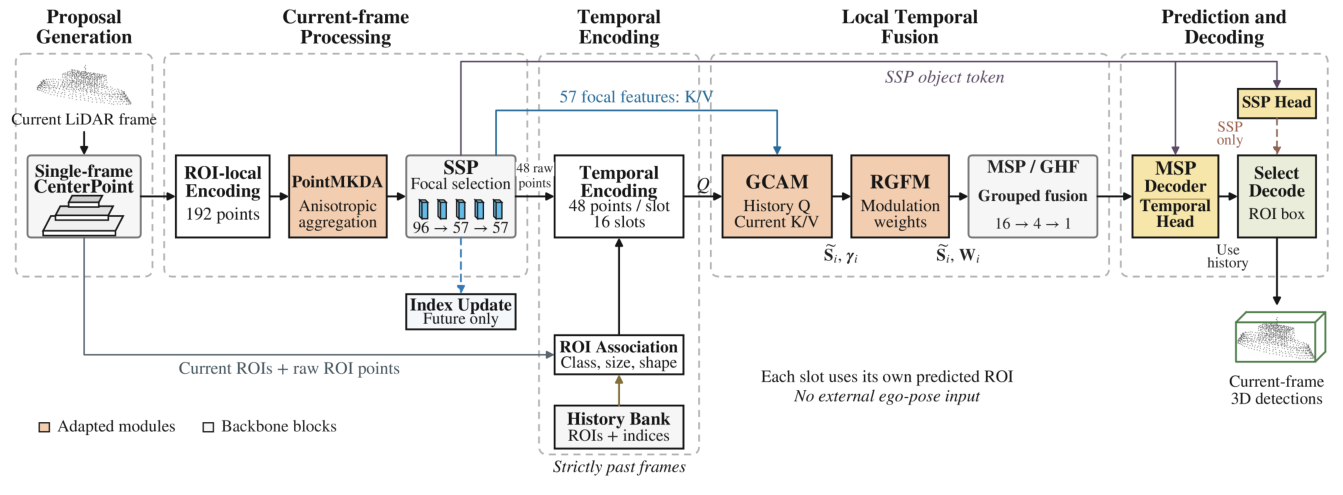
Figure 2.
Structure of PointMKDA and its connection to SSP.
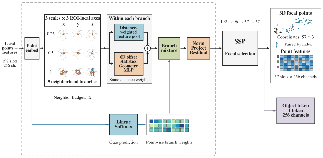
Figure 3.
Structure of GCAM for historical feature updates and geometric support estimation.
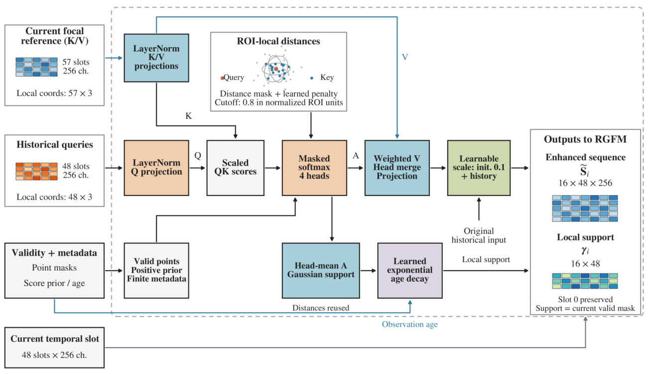
Figure 4.
Structure of RGFM and its connection to MSP.
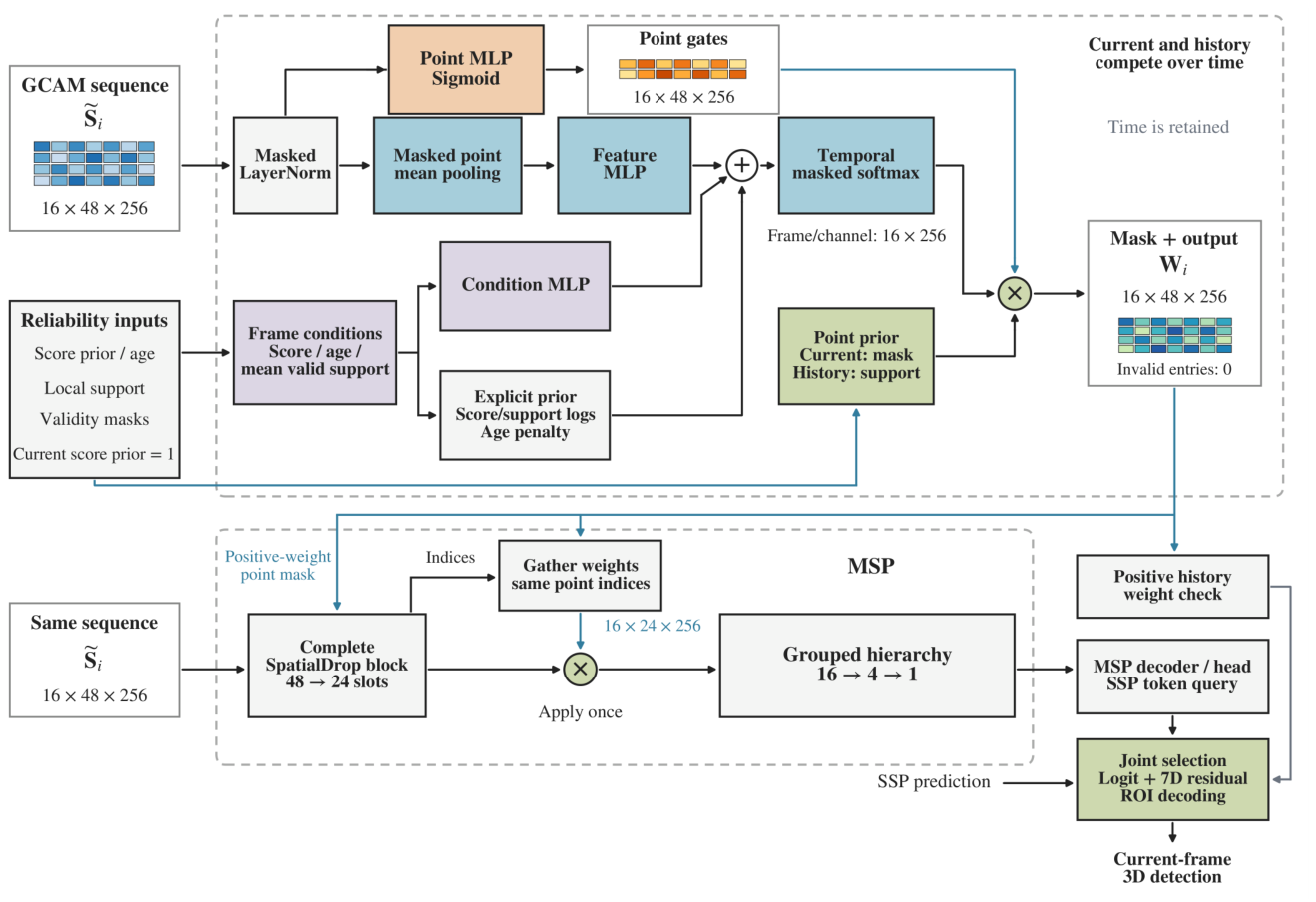
Figure 5.
Paired performance comparison between single-frame and temporal processing.
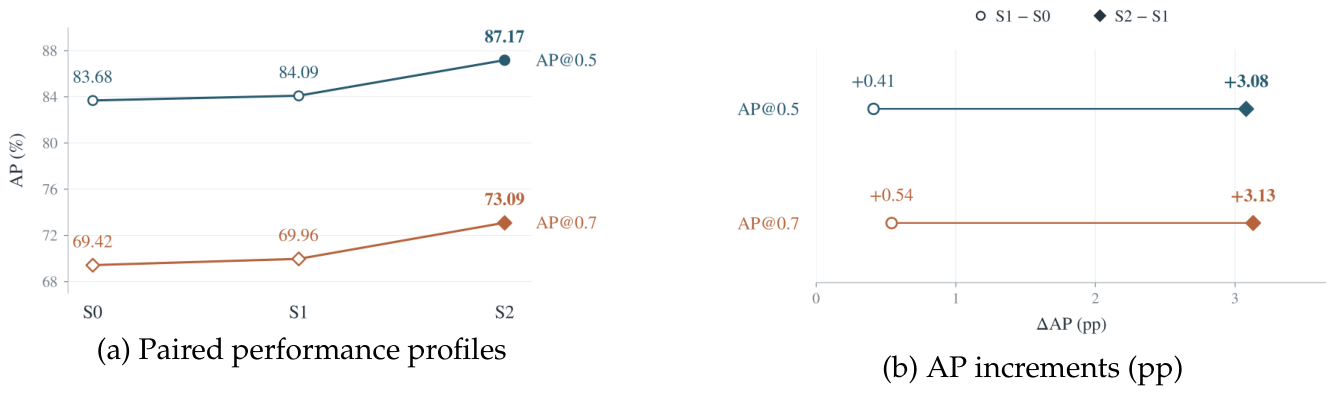
Figure 6.
Effect of history window size on validation AP.
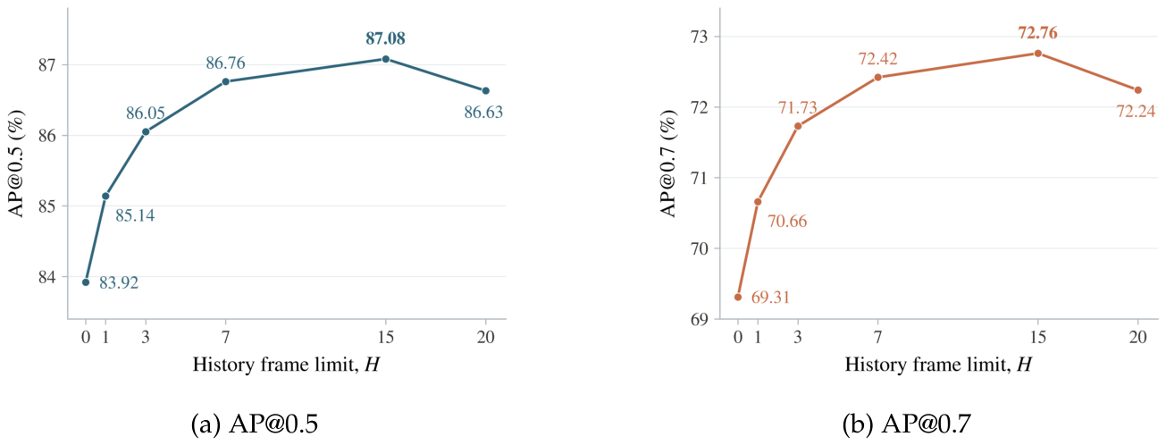
Figure 7.
Comparison of 3D ship detections in representative scenes.
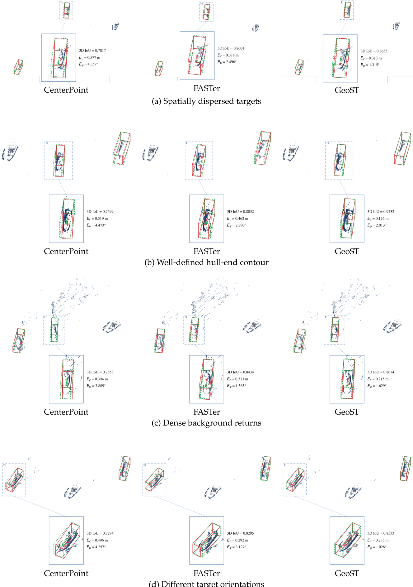
Figure 8.
Comparison of 3D ship detections at four successive time instants.
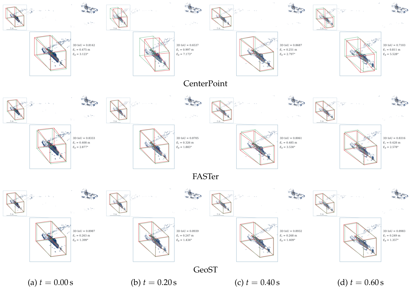

Table 1.
Configurations for the controlled comparison of temporal information.
| Configuration | History duringtraining | History duringevaluation | Output pathway |
|---|---|---|---|
| S0 | Disabled | Disabled | SSP |
| S1 | Enabled | Disabled | SSP |
| S2 | Enabled | Enabled | Temporal branch or SSP |
Table 2.
Validation AP (%) for different history window sizes.
| Maximum number of historical frames H | Maximum total number of frames | AP@0.5 | AP@0.7 |
|---|---|---|---|
| 0 | 1 | 83.92 | 69.31 |
| 1 | 2 | 85.14 | 70.66 |
| 3 | 4 | 86.05 | 71.73 |
| 7 | 8 | 86.76 | 72.42 |
| 15 | 16 | 87.08 | 72.76 |
| 20 | 21 | 86.63 | 72.24 |
Table 3.
Ablation study of PointMKDA, GCAM, and RGFM (AP, %).
| Config. | PointMKDA | GCAM | RGFM | AP@0.5 | AP@0.7 |
|---|---|---|---|---|---|
| B0 | × | × | × | 83.12 | 69.26 |
| B1 | × | × | 84.47 | 70.51 | |
| B2 | × | × | 84.16 | 70.63 | |
| B3 | × | × | 83.82 | 69.94 | |
| B4 | × | 85.63 | 71.92 | ||
| B5 | × | 85.81 | 71.76 | ||
| B6 | × | 86.28 | 72.41 | ||
| B7 | 87.17 | 73.09 |
Table 4.
Detection performance of the compared methods on the test set (%).
| Method | Frames | Overall | L1 | L2 |
|---|---|---|---|---|
| AP@0.5 / AP@0.7 | AP@0.5 / AP@0.7 | AP@0.5 / AP@0.7 | ||
| CenterPoint | 1 | 78.83 / 62.14 | 86.72 / 73.58 | 68.41 / 47.96 |
| VoxelNeXt | 1 | 80.74 / 64.38 | 88.32 / 74.91 | 70.56 / 50.82 |
| DSVT | 1 | 80.19 / 65.07 | 87.95 / 75.36 | 71.03 / 52.14 |
| MPPNet | 16 | 82.61 / 68.26 | 89.24 / 77.53 | 73.58 / 56.07 |
| MSF | 16 | 82.08 / 67.93 | 88.91 / 77.18 | 74.16 / 56.92 |
| PTT | 16 | 83.47 / 69.04 | 89.68 / 78.03 | 76.35 / 59.74 |
| FASTer | 16 | 84.36 / 70.82 | 90.13 / 78.57 | 77.42 / 60.83 |
| GeoST | 16 | 87.17 / 73.09 | 93.48 / 81.22 | 80.26 / 64.47 |
Disclaimer/Publisher’s Note: The statements, opinions and data contained in all publications are solely those of the individual author(s) and contributor(s) and not of MDPI and/or the editor(s). MDPI and/or the editor(s) disclaim responsibility for any injury to people or property resulting from any ideas, methods, instructions or products referred to in the content. |
© 2026 by the authors. Licensee MDPI, Basel, Switzerland. This article is an open access article distributed under the terms and conditions of the Creative Commons Attribution (CC BY) license (http://creativecommons.org/licenses/by/4.0/).
Copyright: This open access article is published under a Creative Commons CC BY 4.0 license, which permit the free download, distribution, and reuse, provided that the author and preprint are cited in any reuse.