

Submitted:
26 October 2026
Posted:
27 October 2026
You are already at the latest version
Abstract
Masked diffusion language models repeatedly compute representations for unresolved tokens, but conventional denoisers do not explicitly retain these representations for reuse across steps. We introduce Temporal Self-Conditioning Diffusion Language Model (TDLM), which lets each unresolved position attend to its own history of hidden representations within a frozen denoiser. This gives later predictions access to computation already performed. Training uses self-generated trajectories and a simple cross-entropy objective for tokens revealed between consecutively sampled decoding steps, while causal temporal attention permits parallel evaluation during training. On LLaDA, the temporal modules add only approximately 0.84% trainable parameters. Across LLaDA and Dream, the main comparison shows up to 7.15× faster generation than the corresponding original diffusion language model, with competitive answer quality on the evaluated tasks. These results motivate temporal memory as a practical way to make more effective use of repeated denoising computation.
Keywords:
masked diffusion language models
; temporal self-conditioning
; temporal memory
; representation reuse
; efficient inference
1. Introduction
Masked diffusion language models offer a route to parallel text generation: a bidirectional denoiser predicts multiple missing tokens, and a decoding policy decides which predictions to commit. LLaDA, iLLaDA, and Dream demonstrate the capabilities of diffusion language modeling at billion-parameter scale [13,14,19]. Nemotron-Labs-Diffusion and DiffusionGemma further develop efficient parallel generation while retaining support for autoregressive decoding [4,6]. The practical efficiency of diffusion generation depends on how many predictions can be committed reliably at each step. Committing too few requires repeated expensive forward passes; committing uncertain predictions can damage the entire answer. Confidence-based decoding exposes this tension directly through a threshold controlling parallelism [17].
Consider a token position that remains masked across several denoising steps. Its discrete input has not changed, yet the model has repeatedly computed a rich representation of what could belong there. As other tokens become visible, these representations evolve. A conventional denoiser carries committed tokens into the next step, but provides no explicit route for an unresolved position to consult its earlier representations. The computation spent on these intermediate estimates has no persistent representation available for direct reuse.
This suggests a question about the use of inference computation: can a denoiser reuse its earlier internal estimates to reach reliable predictions sooner? Historical representations do not provide new external evidence beyond the request and evolving response. Their potential value lies in preserving computations that the model has already performed under earlier contexts. If these computations help resolve uncertainty, more tokens may be committed per evaluation without a corresponding loss in answer quality. If they merely increase confidence, apparent acceleration may instead conceal additional errors. Both possibilities must be tested.
We introduce TDLM, a temporal self-conditioning extension to a pretrained diffusion language model. At selected Transformer layers, each unresolved position attends to its own representations from earlier denoising steps. This preserves the alignment between a pending prediction and the history used to refine it. Narrow temporal projections keep the adaptation small, while a learned zero-value sink allows the model to suppress unhelpful history. The backbone remains frozen. During blockwise generation, unresolved positions continue to accumulate history across block boundaries.
The training procedure is simple: the frozen backbone generates its own trajectories, and the added modules learn to predict the tokens revealed between consecutively sampled decoding steps using cross-entropy. This reuses the backbone’s existing capabilities and the memory accumulated during denoising, while updating only a small set of parameters. It requires no new manually annotated reference answers. Strictly causal temporal attention permits the corresponding partially masked inputs to be evaluated in parallel during training.
Our experiments on LLaDA and Dream study generation efficiency, answer quality, and the role of the available history. Figure 1 illustrates the resulting quality–latency trade-off. We examine whether temporal reuse makes additional computation useful before a token is committed, and how restricting that history changes the model’s predictions.
Our contributions are:
- A lightweight, position-aligned temporal attention mechanism that makes earlier denoising representations available to unresolved predictions in a frozen language model.
- A simple cross-entropy self-distillation objective for earlier prediction, with causal parallel evaluation of sampled trajectory inputs.
- An empirical study of the quality–latency trade-off and the effects of restricting the history available to unresolved predictions.
2. Method
TDLM lets each masked token position reuse hidden representations from earlier denoising steps. Spatial attention exchanges information across positions in the current input; temporal attention retrieves earlier representations of the same position. The backbone remains frozen, and only the added temporal modules are trained.
2.1. Conditioning on Denoising History
Let c be a prompt and N the response length. Each decoding step evaluates the denoiser and reveals one or more tokens: their masks are replaced with predicted tokens, which are then kept fixed. We refer to this operation as commitment.
We call a partially revealed response sequence a state and write it as . Its associated global decoding step is the number of updates already completed. Thus, i indexes the selected sequences, records their times along the decoding trajectory, and p denotes a token position. During training we select a subset of teacher decoding steps; during inference we evaluate every successive input. The initial sequence is at .
For a masked position p, TDLM extends the information available to predict its token :
where denotes the frozen backbone parameters, the temporal parameters, and the hidden representations retained from earlier evaluated inputs , . The input at position p can remain a mask while its internal representation changes with the surrounding context. Temporal memory makes those earlier representations available to the next prediction.
2.2. Temporal Attention at Masked Token Positions
At a selected layer ℓ, let be the hidden representation at position p, after spatial attention and before the feed-forward sublayer. Define and let count the revealed response tokens in . A decoding step can reveal several tokens, so need not equal the step number .
For a currently masked position, every earlier input also masks that position because revealed tokens are never remasked. Its layer-specific history contains earlier representations and their progress coordinates , with . The current representation queries this history through a residual update:
TempAttn uses standard multi-head attention with narrow projections, retrieving only earlier representations of the same token position at the same layer. Temporal rotary embeddings [16] use revealed-token counts to encode decoding progress. A learned attention sink with zero value gives the module an option to ignore history. Appendix B.1 gives the projection, normalization, and multi-head formulas.
Figure 2.
Reusing computation before commitment. Each column is a denoising evaluation, read from bottom to top. The bottom shows the partially revealed input; the top shows token predictions before commitment. Decoding Steps 1–3 use inputs at , respectively. The green position remains masked while its predictions can change. Green arrows retrieve earlier hidden representations at that position and layer. Yellow modules are trainable, and the backbone is frozen.
Figure 2.
Reusing computation before commitment. Each column is a denoising evaluation, read from bottom to top. The bottom shows the partially revealed input; the top shows token predictions before commitment. Decoding Steps 1–3 use inputs at , respectively. The green position remains masked while its predictions can change. Green arrows retrieve earlier hidden representations at that position and layer. Yellow modules are trainable, and the backbone is frozen.
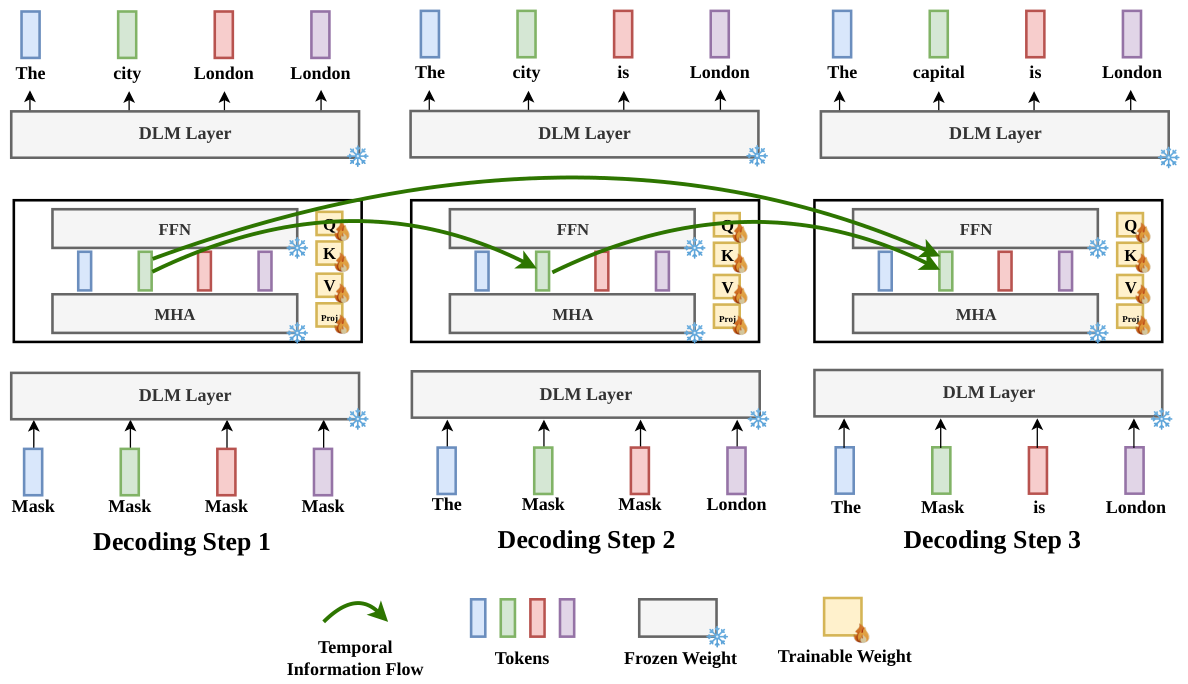
The original feed-forward sublayer processes the corrected representation . Keys and values are formed from h before the same layer’s temporal correction, a property used by parallel trajectory training below. Only masked token positions receive a correction. Empty history produces zero correction, and a zero-initialized output projection preserves the pretrained denoiser at initialization. The precise statements and proofs are in Appendix B.
2.3. Simple Trajectory Self-Distillation
For each prompt, the frozen backbone generates a teacher response in T decoding steps. We record the final tokens and the step at which each token is revealed. These records let us reconstruct the input at any selected step : tokens revealed by that step are visible, and later tokens remain masked,
Hidden representations are computed during training from these reconstructed inputs.
We always include , sample distinct steps uniformly from , and sort them. We also set to mark the end of the trajectory:
The gap is the number of decoding steps between two selected sequences. Every decoding step reveals at least one token, so the number of masks strictly decreases from to . We evaluate ; the fully revealed only marks the end of the last supervision interval and requires no forward pass.
For an input , the training targets are positions that are still masked in but revealed in the next selected sequence . For example, if and , we train the model to predict the tokens the teacher reveals at steps 3 and 4. Positions revealed later remain masked and contribute temporal history, but receive no loss on this input. Formally, the target positions are
The initial input seeds temporal memory without supervision because its temporal correction is zero.
Let be TDLM’s predicted token distribution at position p, conditioned on c, , and . We optimize only , using cross-entropy averaged over all supervised token positions across the sampled inputs:
Each supervised token has equal weight. This objective teaches the model to predict the next interval’s tokens using the current input and its accumulated history. Figure 3 illustrates the inputs and targets; Appendix A gives training details.
Parallel evaluation along a fixed trajectory. Spatial attention processes each reconstructed input independently. At a temporal layer, the causal mask lets the representation for retrieve from earlier inputs where position p was masked. Equation (2) restricts the correction to currently masked positions. Since each layer’s keys and values precede its temporal correction, all sampled inputs can be evaluated together layer by layer. With identical history selection and dropout disabled, this is equivalent in exact arithmetic to processing the same inputs sequentially (Appendix B). Training computes no representations for unsampled steps; inference instead accumulates history from each actual forward pass.
2.4. From Retrieval to Fewer Evaluations
At inference, let be the set of masked token positions in the active block. For the current input , let be the greedy prediction at position p and its confidence. The decoder reveals tokens with confidence above a threshold , or the most confident token otherwise:
TDLM and our Fast-dLLM policy baseline share this commitment rule. Original DLM reveals one token per evaluation. Decoding settings are specified together in Section 3.1.
Each forward pass retrieves earlier temporal keys and values, then appends the current entries. All masked response positions accumulate history, including those outside the active block. Revealing a token invalidates that position’s history; changing blocks does not reset the histories of other positions. The full spatial sequence is recomputed at every step.
With temporal layers and total temporal width , the module parameter count is . Retrieving from H earlier evaluations costs per temporal layer, in addition to the projections. Full-history memory requires storage, and unrestricted attention work grows quadratically with the number of denoising steps. TDLM is therefore useful when it saves enough backbone evaluations to offset this overhead. We measure both evaluation counts and wall time, together with answer quality, to assess that trade-off.
3. Experiments
We evaluate the quality–latency trade-off of TDLM on two backbones and study the contribution of its temporal history.
3.1. Experimental Setup
Models and training. We augment frozen LLaDA-8B-Instruct and Dream-v0-Instruct-7B backbones. LLaDA uses sixteen dispersed temporal layers with four heads of width 64; Dream uses fourteen middle layers with four heads of width 84. For each backbone, we train only the temporal modules on 3,500 self-generated trajectories for 750 optimizer updates using the simple CE objective in Eq. (5). These results therefore require a modest adaptation dataset and a straightforward self-distillation procedure. Appendix A gives the model and training details. Our MetaState baseline uses reference responses from the Tulu-3 SFT mixture as supervision [18], whereas TDLM learns from responses generated by its own frozen backbone.
Tasks and scoring. We evaluate mathematical reasoning on MATH-500 and GSM8K, and code generation on MBPP sanitized [1,3,7,9]. We use the complete test sets of 500, 1,319, and 257 problems, respectively. Math answers are checked with Math-Verify, and code solutions are executed against the dataset tests. We report accuracy or pass@1 from one greedy generation per problem; unparseable answers count as incorrect.
Decoding and measurement. All methods in the main comparison use a generation budget of 256 tokens and block size 32. Confidence-based decoding uses , following released evaluation settings [11,17]; d3LLM uses its default entropy threshold [15]. On Dream, TDLM uses and d3LLM uses . Original DLM commits one token per evaluation. All methods use compiled model forwards with batch size one on GH200 GPUs. We report mean denoiser evaluations (NFE) and generation seconds, excluding compilation and warmup. Speedup is measured against the original model of the same backbone on the same task. Further evaluation details are in Appendix C.
3.2. Generation Efficiency and Answer Quality
Table 1 compares both backbones across the three tasks. TDLM achieves up to 7.15× faster generation than original DLM in the main comparison, and up to 1.85× over Fast-dLLM. Its largest score improvement over Fast-dLLM is 2.72 percentage points on LLaDA MBPP. Across the six backbone–task combinations, TDLM ranks first, second, and third in quality in one, four, and one cases, respectively; the corresponding latency counts are three, two, and one, using the table’s tie convention. Quality changes remain task-dependent.
Figure 1 compares generation quality and latency across decoding thresholds to explore the empirical Pareto frontier. TDLM pushes the Pareto frontier, offering higher accuracy at fast speeds. Appendix F extends the LLaDA evaluation to 128- and 384-token generation budgets, with speedups over original DLM reaching 8.54× at the longer budget.
3.3. What Does Temporal History Contribute?
We keep the LLaDA checkpoint fixed and vary the context available to the temporal modules: representations from the current evaluation only, the previous one, three or five evaluations, or the complete history. Table 2 reports these inference-time restrictions. The current-only condition retains the learned Q/K/sink gate.
Extending history from one evaluation to the complete trajectory raises observed accuracy from 77.62% to 79.08%, while reducing NFE from 44.06 to 40.08 and mean time from 0.637 to 0.585 seconds. Current-only inference achieves 76.48% accuracy with 42.64 evaluations. These measurements show how the available history changes predictions and commitment behavior for a fixed checkpoint. Implementation details and architecture comparisons are given in Appendices Appendix E and Appendix D.
4. Related work
Parallel decoding and diffusion acceleration. Fast-dLLM [17] combines confidence-based parallel decoding with KV-cache reuse. dKV-Cache [12] uses delayed and conditioned caching to reuse key and value states during denoising. Training-based methods include CDLM [11], which combines consistency training with blockwise causal attention, and d3LLM [15], which uses pseudo-trajectory distillation and entropy-based multi-block decoding. TDLM studies position-aligned temporal retrieval as a way to make earlier denoising computations useful for later predictions.
Self-conditioning and persistent representations. Analog Bits [2] conditions diffusion predictions on earlier model predictions. Recurrent Interface Networks [10] introduce latent self-conditioning across reverse diffusion steps for image and video generation. In language models, RCD [8] recycles discarded-token representations as residual context for subsequent denoising. MetaState [18] equips a frozen discrete diffusion model with fixed-size recurrent working memory, while ALoDLM [5] uses token-adaptive latent recurrence. TDLM retrieves an explicit history of same-position representations at multiple layers of a frozen backbone, with simple trajectory self-distillation and causal parallel evaluation of sampled trajectory inputs.
5. Discussion and Future Work
Temporal memory provides a way to use earlier denoising computations when predicting unresolved tokens. The generation and history-restriction experiments show how this changes the balance between answer quality and the number of evaluations. Further analysis of token-level correctness and confidence, together with a capacity-matched adapter using only the current hidden representation, would help characterize when history is most useful.
Self-distillation inherits the quality limitations of the teacher-generated trajectories. With a frozen backbone and teacher tokens drawn from its own outputs, supervision offers limited evidence for correcting systematic teacher errors. Teacher capability therefore provides a practical reference for the quality available through this training signal. Future work can explore higher-quality training data and full-model fine-tuning, allowing the backbone and temporal attention to adapt jointly and make better use of the accumulated memory.
Sparse teacher trajectories and the student’s own multi-token commitments can expose the model to different histories. Longer responses, repeated measurements, and combinations with spatial KV caching and early stopping are additional directions for evaluation.
6. Conclusion
TDLM augments a frozen diffusion language model with lightweight attention over the history of unresolved positions. A simple trajectory self-distillation objective trains earlier predictions, while causal temporal attention permits parallel evaluation of sampled trajectory inputs. The available experiments show that fewer backbone evaluations can outweigh the added temporal computation at useful quality levels. Reusing denoising history thus offers a practical direction for improving generation efficiency through the model’s existing capabilities.
Appendix A. Training Details
For each backbone, we train the temporal modules on 3,500 self-generated trajectories for 750 optimizer updates with the interval-only CE objective in Eq. (5). Backbone parameters remain frozen throughout training. The modules are initialized with a zero output projection, and sampled inputs are evaluated with causal temporal attention.
LLaDA. Temporal modules are installed at zero-based layer indices . Each uses four heads of width 64 and unrestricted history, adding 67,108,880 parameters, approximately 0.84% of the nominal 8B backbone.
Dream. Temporal modules occupy the middle fourteen layers, at zero-based indices 7–20, with four heads of width 84 and unrestricted history. Predicting the token at position p uses the hidden representation at position ; temporal memory and commitment masks are aligned to the response token position, including the first response token.
Additional optimization details. Prompt source and filtering: . Optimizer and learning-rate schedule: . Batch size and sampled inputs per trajectory: . Validation and checkpoint selection: .
Trainable parameters and data scale.Table 3 compares the added trainable parameters and training-data volume of the LLaDA-based methods. TDLM trains 67.11M temporal-module parameters on 3,500 self-generated trajectories while keeping the backbone frozen. The data counts retain each method’s unit: examples, prompts, or trajectories.

Table 3.
Added trainable parameters and training-data scale for LLaDA-based models. M denotes one million parameters.
Table 3.
Added trainable parameters and training-data scale for LLaDA-based models. M denotes one million parameters.
| Method | Added trainable parameters |
Training data |
|---|---|---|
| d3LLM [15] | 335.54M (LoRA) | ≈92k examples |
| CDLM [11] | 176.13M (LoRA) | ≈15k prompts; trajectories collected at two temperatures per prompt |
| MetaState [18] | 51.08M | 15,543 instruction–response examples |
| TDLM | 67.11M | 3,500 self-generated trajectories |
Appendix B. Properties of Temporal Evaluation
Appendix B.1. Temporal Attention Operator
We use the notation of Section 2: is the selected input at decoding step , p is a token position, and is its hidden representation at layer ℓ. Each temporal module has M heads of width , with total width . Head a uses bias-free projections :
applies temporal RoPE within each head. Its rotation angles are , with for . The relative positional term depends on , while the hidden representations and available histories can still differ across decoding schedules.
Let contain the indices of earlier evaluated inputs retained as history for masked position p. The attention score and normalizer are
Here is a learned sink logit shared by the heads; its value vector is zero. Each head retrieves
The operator in Eq. (2) is
All keys and values use the residual representation before this layer’s temporal correction. The resulting correction is . This explicit form gives the same update as the compact operator in the main text.
Appendix B.2. Sink, Cold Start, and Initialization
The sink probability in head a is
Its history weights sum to . If for every head and available history, then
This follows directly from the triangle inequality and the nonnegative attention weights. The sink therefore gates the magnitude of the retrieved history without a separate gating network. This is a local bound on the module output, not a guarantee of whole-model stability or accuracy.
Proposition 1
(Cold start and initialization). For history-only temporal attention, the first forward pass of each request has zero temporal correction at every layer. If each is initialized to zero, the entire initialized TDLM denoiser equals the backbone on every input along any fixed trajectory, in exact arithmetic.
Proof.
On the first pass, is empty, so the only attention entry is the zero-value sink. At initialization, multiplication by removes the correction even when history is available. Induction over backbone layers gives identical representations and output distributions. □
Appendix B.3. Parallel and sequential evaluation
Proposition 2
(Parallel evaluation on a fixed trajectory). With dropout disabled and identical history selection, evaluating the sampled inputs together using A gives the same outputs as evaluating those inputs sequentially with temporal caches, in exact arithmetic.
Proof.
The input embeddings agree for each . Suppose the representations agree at the input to a layer. Spatial attention processes each sequence independently, so the post-attention representations also agree. Keys and values are computed before the temporal correction at this layer. The parallel mask therefore selects exactly the keys and values that sequential evaluation would have cached from earlier sampled inputs. The temporal update and the unchanged feed-forward sublayer then give the same layer outputs. Induction over layers establishes the claim. □
This equivalence concerns a fixed set of sampled inputs. No hidden representations are computed or inserted into memory for unsampled decoding steps. Training histories and those accumulated during generation can consequently differ. Although backbone weights are frozen, gradients still propagate through later backbone computations to train the temporal modules.
Appendix C. Evaluation Details
Answer scoring. MATH-500 and GSM8K prompts request a solution ending in a boxed answer. The last boxed answer is checked for mathematical equivalence using Math-Verify 0.8.0. MBPP prompts request complete Python code with a signature derived from the reference implementation, without exposing the function body or tests. Extracted code is checked against the dataset tests with a three-second timeout and a 512 MB memory limit. Failed or unparseable answers count as incorrect. Scoring uses the text before the first EOS/EOT marker.
For the dagger-marked Dream MetaState scores in Table 1, scoring removes only the literal strings <tool_call> and </tool_call>. Its raw MBPP pass@1 is 23.74%, compared with 58.37% after this treatment. NFE and latency use the original generations.
Runtime measurement. The experiments use PyTorch 2.9.0+cu128 and compiled generation. TDLM uses a fused temporal kernel and BF16 temporal keys and values. Timing covers the full generation budget and excludes compilation, warmup, tokenization, external text decoding, and grading. Measurements come from separate GH200 jobs, with one timed generation per problem. Native decoder-loop work is included where present.
TDLM, Fast-dLLM and original LLaDA each use eager fallback for four long MATH-500 prompts; MetaState compiles the full LLaDA test set. The Dream runs use three long-prompt fallbacks per method. These implementation details are included in the measured latency.
Appendix D. Architecture Ablations on GSM8K
We compare temporal-layer allocations and widths using LLaDA-8B-Instruct on all 1,319 GSM8K test problems. All measured configurations use the main GSM8K settings in Section 3.1. NFE and average seconds are means per problem; timing covers full-budget generation without EOS early stopping and excludes compilation and warmup. Measurements come from separate GH200 jobs, so small timing differences are approximate.
Appendix D.1. Different Temporal-Layer Allocations
Table 4 favors sixteen dispersed layers, used for the main LLaDA results, among the measured allocations. They achieve 79.08% accuracy versus 77.86% for eight dispersed layers, at similar NFE and latency. Sixteen middle layers achieve nearly identical accuracy (79.00%), but require 45.72 NFE and 0.683 seconds, compared with 40.08 NFE and 0.585 seconds for the dispersed allocation. The thirty-two-layer configuration has no task-level measurements. Its training OOM status was supplied by the authors; a corresponding log is not included in the evidence snapshot.
Table 4.
Different temporal-layer allocations on GSM8K. Every temporal module uses four heads of width 64; measured models share the 750-update training recipe.
Table 4.
Different temporal-layer allocations on GSM8K. Every temporal module uses four heads of width 64; measured models share the 750-update training recipe.
| Temporal layers | Accuracy (%) | NFE | Avg. sec |
|---|---|---|---|
| 8, dispersed | 77.86 | 40.15 | 0.571 |
| 16, middle | 79.00 | 45.72 | 0.683 |
| 16, dispersed (main) | 79.08 | 40.08 | 0.585 |
| 32, all | Training OOM | ||
Appendix D.2. Temporal Width and Head Configurations
In Table 5, the single-head runs use 500 updates, include 192-token training trajectories, and differ in length-sampling weights and lookahead scheduling. The multi-head runs use 750 updates and 128/256-token trajectories. Thus, the full table does not isolate width from training-recipe differences. The two width-256 rows do share training settings: four heads of width 64 achieve 79.00% accuracy versus 78.47% for two heads of width 128, with similar NFE and latency. These single-run differences do not establish statistical significance.
Table 5.
Temporal-width and head configurations on GSM8K. All models augment the middle sixteen backbone layers (zero-based indices 8–23). Total width is the product of head count and head width. Training-recipe differences are described in the text.
Table 5.
Temporal-width and head configurations on GSM8K. All models augment the middle sixteen backbone layers (zero-based indices 8–23). Total width is the product of head count and head width. Training-recipe differences are described in the text.
| Heads × head width | Total width | Updates | Accuracy (%) | NFE | Avg. sec |
|---|---|---|---|---|---|
| 64 | 500 | 76.35 | 47.34 | 0.682 | |
| 128 | 500 | 77.71 | 47.66 | 0.701 | |
| 256 | 750 | 78.47 | 45.84 | 0.688 | |
| 256 | 750 | 79.00 | 45.72 | 0.683 |
Appendix E. Temporal Context During Inference on GSM8K
The recorded intervention reuses the main checkpoint with sixteen dispersed layers and four heads of width 64. Temporal context is restricted to representations from the current evaluation only, the previous one, three or five evaluations, or the complete history. Current-only attention retains the learned Q/K/sink gate. All uncommitted positions retain their allowed histories across block boundaries. The evaluation follows Section 3.1.
Finite windows use circular K/V slots per uncommitted position. Complete history grows in pages of eight steps, with pages returned to the allocator after commitment. A fixed device page table permits CUDA Graph reuse. GPU memory denotes the maximum question-level allocated memory after warmup, including weights and workspaces.
Table 2 reports the available measurements. Within the historical-window conditions, accuracy increases from 77.62% with one previous evaluation to 79.08% with complete history, while NFE decreases from 44.06 to 40.08. Current-only uses the original temporal implementation, while the historical-window conditions use paged K/V storage. Each condition is evaluated without retraining the temporal modules.
Appendix F. Generation Lengths on LLaDA
Table 6 and Table 7 extend the LLaDA evaluation to generation budgets of 128 and 384 tokens, respectively, with block size fixed at 32. At 128 tokens, TDLM achieves 3.50–4.84× speedups over original DLM across MATH-500, GSM8K and MBPP, with score differences of , and percentage points relative to Fast-dLLM. At 384 tokens, the corresponding speedups over original DLM are 4.81–8.54×, with score differences of , and points relative to Fast-dLLM. TDLM uses fewer evaluations and less time than Fast-dLLM in all six comparisons. These results extend the measured quality–latency trade-off across generation budgets, while the MBPP decrease at 384 tokens illustrates that quality changes remain task-dependent.
Table 6.
LLaDA with a 128-token generation budget and block size 32. ACC is mathematical accuracy or code pass@1. Speedup is relative to original DLM on the same task at this budget. Medal colors and ties follow Table 1. Values and speedup ratios are reported at the supplied precision.
Table 6.
LLaDA with a 128-token generation budget and block size 32. ACC is mathematical accuracy or code pass@1. Speedup is relative to original DLM on the same task at this budget. Medal colors and ties follow Table 1. Values and speedup ratios are reported at the supplied precision.
| Dataset | Model | ACC (%) ↑ | NFE | Sec. ↓ | Speedup |
|---|---|---|---|---|---|
| MATH-500 | TDLM | 36.00 | 32.60 | 0.366 | 3.50× |
| Fast-dLLM | 36.40 | 64.28 | 0.670 | 1.91× | |
| MetaState | 35.80 | 65.14 | 0.742 | 1.72× | |
| CDLM | 30.80 | 46.36 | 1.806 | 0.71× | |
| d3LLM | 31.40 | 42.96 | 0.947 | 1.35× | |
| Original DLM | 36.00 | 128.00 | 1.281 | 1.00× | |
| GSM8K | TDLM | 73.74 | 26.67 | 0.282 | 4.33× |
| Fast-dLLM | 73.09 | 52.85 | 0.520 | 2.35× | |
| MetaState | 71.04 | 53.25 | 0.580 | 2.11× | |
| CDLM | 2.12 | 40.54 | 1.476 | 0.83× | |
| d3LLM | 66.41 | 37.82 | 0.698 | 1.75× | |
| Original DLM | 73.16 | 128.00 | 1.223 | 1.00× | |
| MBPP | TDLM | 45.91 | 23.82 | 0.233 | 4.84× |
| Fast-dLLM | 45.53 | 26.96 | 0.242 | 4.67× | |
| MetaState | 45.53 | 30.09 | 0.305 | 3.71× | |
| CDLM | 45.14 | 25.05 | 0.919 | 1.23× | |
| d3LLM | 45.53 | 21.02 | 0.426 | 2.65× | |
| Original DLM | 44.75 | 128.00 | 1.130 | 1.00× |
Table 7.
LLaDA with a 384-token generation budget and block size 32. ACC is mathematical accuracy or code pass@1. Speedup is relative to original DLM on the same task at this budget. Medal colors and ties follow Table 1. Values and speedup ratios are reported at the supplied precision.
Table 7.
LLaDA with a 384-token generation budget and block size 32. ACC is mathematical accuracy or code pass@1. Speedup is relative to original DLM on the same task at this budget. Medal colors and ties follow Table 1. Values and speedup ratios are reported at the supplied precision.
| Dataset | Model | ACC (%) ↑ | NFE | Sec. ↓ | Speedup |
|---|---|---|---|---|---|
| MATH-500 | TDLM | 42.80 | 70.83 | 1.389 | 4.81× |
| Fast-dLLM | 41.60 | 134.01 | 2.443 | 2.73× | |
| MetaState | 41.20 | 135.23 | 2.599 | 2.57× | |
| CDLM | 31.00 | 91.48 | 3.569 | 1.87× | |
| d3LLM | 35.80 | 42.06 | 1.618 | 4.12× | |
| Original DLM | 43.20 | 384.00 | 6.675 | 1.00× | |
| GSM8K | TDLM | 80.83 | 48.32 | 0.898 | 7.09× |
| Fast-dLLM | 80.74 | 90.62 | 1.557 | 4.09× | |
| MetaState | 81.27 | 93.51 | 1.700 | 3.75× | |
| CDLM | 68.84 | 72.06 | 2.811 | 2.27× | |
| d3LLM | 78.85 | 36.21 | 1.032 | 6.18× | |
| Original DLM | 81.20 | 384.00 | 6.370 | 1.00× | |
| MBPP | TDLM | 45.58 | 40.19 | 0.725 | 8.54× |
| Fast-dLLM | 46.30 | 51.97 | 0.864 | 7.16× | |
| MetaState | 45.53 | 66.31 | 1.178 | 5.26× | |
| CDLM | 45.91 | 35.03 | 1.344 | 4.61× | |
| d3LLM | 43.58 | 28.26 | 1.098 | 5.64× | |
| Original DLM | 45.53 | 384.00 | 6.191 | 1.00× |
References
- Jacob Austin, Augustus Odena, Maxwell Nye, Maarten Bosma, Henryk Michalewski, David Dohan, Ellen Jiang, Carrie Cai, Michael Terry, Quoc Le, and Charles Sutton. Program synthesis with large language models. arXiv preprint arXiv:2108.07732, 2021. URL https://arxiv.org/abs/2108.07732.
- Ting Chen, Ruixiang Zhang, and Geoffrey Hinton. Analog bits: Generating discrete data using diffusion models with self-conditioning. In International Conference on Learning Representations, 2023. URL https://arxiv.org/abs/ 2208.04202.
- Karl Cobbe, Vineet Kosaraju,Mohammad Bavarian,Mark Chen, Heewoo Jun, Lukasz Kaiser,Matthias Plappert, Jerry Tworek, Jacob Hilton, Reiichiro Nakano, Christopher Hesse, and John Schulman. Training verifiers to solve math word problems. arXiv arXiv:2110.14168, 2021. https://arxiv.org/abs/2110.14168.
- DiffusionGemma Team et al. DiffusionGemma technical report. arXiv:2608.00146, 2026. URL https: //arxiv.org/abs/2608.00146.
- Liancheng Fang, Zhuowei Li, Youngeun Kim, Tianchen Zhao, Rajat Koner, JiayeWu, Linghan Xu, Xuanbai Chen, Xiang Xu, Zheng Zhang, Jakub Zablocki, Nishant Sankaran, and Yifan Xing. ALoDLM: Adaptively looped diffusion language models. arXiv:2610.04198, 2026. URL https://arxiv.org/abs/2610.04198.
- Yonggan Fu, Lexington Whalen, Abhinav Garg, Chengyue Wu, Maksim Khadkevich, Nicolai Oswald, Enze Xie, Daniel Egert, Sharath Turuvekere Sreenivas, Shizhe Diao, Chenhan Yu, Ye Yu, Weijia Chen, Sajad Norouzi, Jingyu Liu, Shiyi Lan, Ligeng Zhu, Jin Wang, Jindong Jiang, Morteza Mardani, Mehran Maghoumi, Song Han, Ante Juki´c, Nima Tajbakhsh, Jan Kautz, and Pavlo Molchanov. Nemotron-Labs-Diffusion: A trimode language model unifying autoregressive, diffusion, and self-speculation decoding. arXiv:2607.05722, 2026. URL https://arxiv.org/abs/2607.05722.
- Google Research. MBPP sanitized dataset. Hugging Face dataset, sanitized configuration, test split, 2021. Available online: https://huggingface.co/datasets/google-research-datasets/mbpp.
- Yuezhou Hu, Harman Singh, Monishwaran Maheswaran, Haocheng Xi, Coleman Hooper, Jintao Zhang, Aditya Tomar, Michael W. Mahoney, Sewon Min, Mehrdad Farajtabar, Kurt Keutzer, Amir Gholami, and Chenfeng Xu. Residual context diffusion language models. arXiv preprint arXiv:2601.22954, 2026. URL https://arxiv.org/abs/2601.22954.
- Hugging Face H4. MATH-500. Hugging Face dataset, n.d. URL https://huggingface.co/datasets/ HuggingFaceH4/MATH-500.
- Allan Jabri, David Fleet, and Ting Chen. Scalable adaptive computation for iterative generation. arXiv preprint arXiv:2212.11972, 2022. URL https://arxiv.org/abs/2212.11972.
- Minseo Kim, Chenfeng Xu, Coleman Hooper, Harman Singh, Ben Athiwaratkun, Ce Zhang, Kurt Keutzer, and Amir Gholami. CDLM: Consistency diffusion language models for faster sampling. arXiv preprint arXiv:2511.19269, 2025. URL https://arxiv.org/abs/2511.19269.
- Xinyin Ma, Runpeng Yu, Gongfan Fang, and Xinchao Wang. dKV-Cache: The cache for diffusion language models. arXiv preprint arXiv:2505.15781, 2025. URL https://arxiv.org/abs/2505.15781.
- Shen Nie, Fengqi Zhu, Zebin You, Xiaolu Zhang, Jingyang Ou, Jun Hu, Jun Zhou, Yankai Lin, Ji-Rong Wen, and Chongxuan Li. Large language diffusion models. arXiv preprint arXiv:2502.09992, 2025. URL https://arxiv.org/abs/2502.09992.
- Shen Nie, Qiyang Min, Shaoxuan Xu, Zihao Huang, Yuxuan Song, Yong Shan, Yankai Lin, Wayne Xin Zhao, Chongxuan Li, and Ji-Rong Wen. Improved large language diffusion models. arXiv:2606.25331, 2026. URL https://arxiv.org/abs/2606.25331.
- Yu-Yang Qian, Junda Su, Lanxiang Hu, Peiyuan Zhang, Zhijie Deng, Peng Zhao, and Hao Zhang. d3LLM: Ultra-fast diffusion LLM using pseudo-trajectory distillation. arXiv preprint arXiv:2601.07568, 2026. URL https://arxiv.org/abs/2601.07568.
- Jianlin Su, Yu Lu, Shengfeng Pan, Ahmed Murtadha, Bo Wen, and Yunfeng Liu. RoFormer: Enhanced transformer with rotary position embedding. arXiv preprint arXiv:2104.09864, 2021. URL https://arxiv.org/ abs/2104.09864.
- Chengyue Wu, Hao Zhang, Shuchen Xue, Zhijian Liu, Shizhe Diao, Ligeng Zhu, Ping Luo, Song Han, and Enze Xie. Fast-dLLM: Training-free acceleration of diffusion LLM by enabling KV cache and parallel decoding. arXiv preprint arXiv:2505.22618, 2025. URL https://arxiv.org/abs/2505.22618.
- Kejing Xia, Mingzhe Li, LixuanWei, Zhenbang Du, Xiangchi Yuan, Qirui Jin, andWenke Lee. MetaState: Persistent working memory for discrete diffusion language models. arXiv preprint arXiv:2603.01331, 2026. URL https://arxiv.org/abs/2603.01331.
- Jiacheng Ye, Zhihui Xie, Lin Zheng, Jiahui Gao, Zirui Wu, Xin Jiang, Zhenguo Li, and Lingpeng Kong. Dream 7b: Diffusion large language models. arXiv preprint arXiv:2508.15487, 2025. URL https://arxiv.org/ abs/2508.15487.
Figure 1.
Accuracy–latency trade-off on GSM8K. Threshold sweeps compare TDLM with the evaluated baselines.
Figure 1.
Accuracy–latency trade-off on GSM8K. Threshold sweeps compare TDLM with the evaluated baselines.
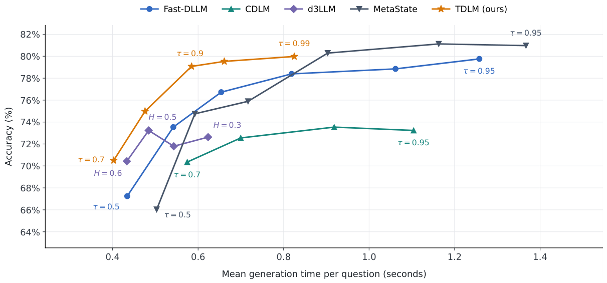
Figure 3.
Sampled inputs and their training targets. The top row gives the teacher’s reveal step for each token position. The three input rows are at steps (labelled in the figure). Gray positions are revealed context. Green positions are masked inputs whose teacher tokens become visible in the next selected sequence and are used as CE targets. Red positions are also masked, but receive no loss on that input. Arrows show reuse of earlier hidden representations at the same position and layer. The initial input is omitted; the final boundary is .
Figure 3.
Sampled inputs and their training targets. The top row gives the teacher’s reveal step for each token position. The three input rows are at steps (labelled in the figure). Gray positions are revealed context. Green positions are masked inputs whose teacher tokens become visible in the next selected sequence and are used as CE targets. Red positions are also masked, but receive no loss on that input. Arrows show reuse of earlier hidden representations at the same position and layer. The initial input is omitted; the final boundary is .
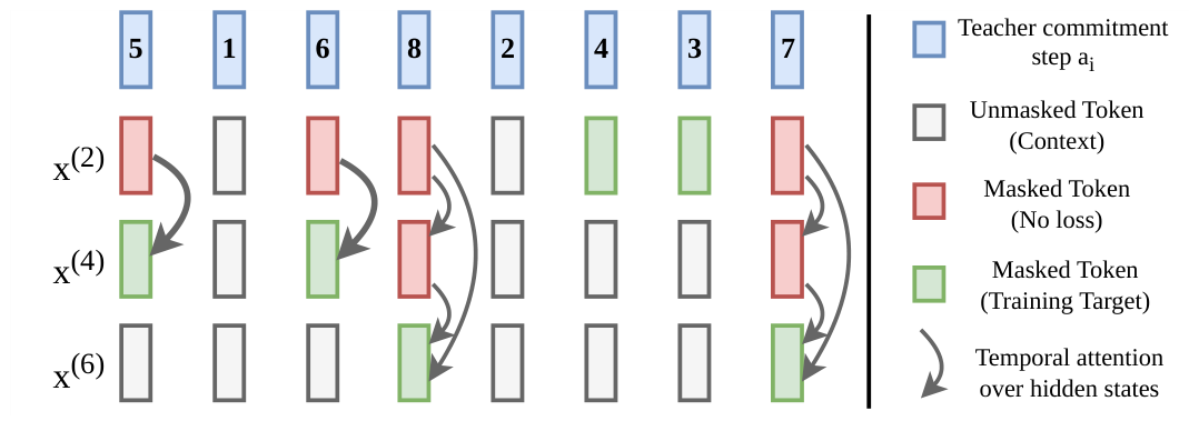
Table 1.
Main results on two backbones. ACC is mathematical accuracy or code pass@1; NFE and seconds are per-problem means. Speedup is relative to the original model of the same backbone on the same task. Gold, silver, and bronze mark the three best distinct displayed values within each backbone–task group; ties share a rank. †: scoring-only tag removal for the Dream MetaState results is described in Appendix C.
Table 1.
Main results on two backbones. ACC is mathematical accuracy or code pass@1; NFE and seconds are per-problem means. Speedup is relative to the original model of the same backbone on the same task. Gold, silver, and bronze mark the three best distinct displayed values within each backbone–task group; ties share a rank. †: scoring-only tag removal for the Dream MetaState results is described in Appendix C.
| LLaDA-8B-Instruct | Dream-v0-Instruct-7B | ||||||||
| Dataset | Model | ACC (%) ↑ | NFE | Sec. ↓ | Speedup | ACC (%) ↑ | NFE | Sec. ↓ | Speedup |
| MATH-500 | TDLM | 37.20 | 54.79 | 0.829 | 4.26× | 44.20 | 74.62 | 1.194 | 3.05× |
| Fast-dLLM | 38.60 | 107.20 | 1.535 | 2.30× | 44.00 | 113.50 | 1.646 | 2.21× | |
| MetaState | 36.80 | 107.56 | 1.682 | 2.10× | 40.80† | 115.88 | 1.671 | 2.18× | |
| CDLM | 30.40 | 87.89 | 2.851 | 1.24× | >26.00 | 96.93 | 1.438 | 2.53× | |
| d3LLM | 31.80 | 35.67 | 1.244 | 2.84× | 42.40 | 53.76 | 0.820 | 4.45× | |
| Original DLM | 38.40 | 256.00 | 3.535 | 1.00× | 44.60 | 256.00 | 3.645 | 1.00× | |
| GSM8K | TDLM | 79.08 | 40.08 | 0.585 | 5.91× | 79.15 | 62.90 | 0.951 | 3.63× |
| Fast-dLLM | 78.85 | 76.72 | 1.062 | 3.26× | 79.00 | 97.35 | 1.329 | 2.60× | |
| MetaState | 81.12 | 77.36 | 1.163 | 2.97× | 75.21† | 101.79 | 1.430 | 2.41× | |
| CDLM | 65.66 | 68.66 | 2.748 | 1.26× | 63.15 | 88.47 | 1.236 | 2.79× | |
| d3LLM | 75.44 | 23.35 | 0.805 | 4.30× | 77.33 | 40.54 | 0.587 | 5.88× | |
| Original DLM | 78.62 | 256.00 | 3.457 | 1.00× | 78.85 | 256.00 | 3.452 | 1.00× | |
| MBPP | TDLM | 46.69 | 36.98 | 0.517 | 6.27× | 57.98 | 31.14 | 0.467 | 7.15× |
| Fast-dLLM | 43.97 | 52.13 | 0.676 | 4.79× | 58.37 | 40.51 | 0.559 | 5.97× | |
| MetaState | 48.64 | 63.91 | 0.917 | 3.53× | 58.37† | 59.88 | 0.837 | 3.99× | |
| CDLM | 45.91 | 32.02 | 1.476 | 2.19× | 50.58 | 29.46 | 0.401 | 8.31× | |
| d3LLM | 45.53 | 25.00 | 0.947 | 3.42× | 55.25 | 24.95 | 0.351 | 9.50× | |
| Original DLM | 44.75 | 256.00 | 3.240 | 1.00× | 58.37 | 256.00 | 3.334 | 1.00× | |
Table 2.
Restricting temporal context at inference. All conditions reuse the same trained LLaDA checkpoint without retraining. Current-only retains the Q/K/sink gate. GPU memory includes weights and compiled workspaces. Implementation details are in Appendix E.
Table 2.
Restricting temporal context at inference. All conditions reuse the same trained LLaDA checkpoint without retraining. Current-only retains the Q/K/sink gate. GPU memory includes weights and compiled workspaces. Implementation details are in Appendix E.
| Temporal context | Accuracy (%) | NFE | Sec. | GPU (GiB) |
|---|---|---|---|---|
| Current only (gated) | 76.48 | 42.64 | 0.623 | 15.184 |
| Last 1 | 77.62 | 44.06 | 0.637 | 15.188 |
| Last 3 | 78.00 | 42.36 | 0.631 | 15.196 |
| Last 5 | 78.68 | 41.57 | 0.601 | 15.204 |
| Full history | 79.08 | 40.08 | 0.585 | 15.330 |
Disclaimer/Publisher’s Note: The statements, opinions and data contained in all publications are solely those of the individual author(s) and contributor(s) and not of MDPI and/or the editor(s). MDPI and/or the editor(s) disclaim responsibility for any injury to people or property resulting from any ideas, methods, instructions or products referred to in the content. |
© 2026 by the authors. Licensee MDPI, Basel, Switzerland. This article is an open access article distributed under the terms and conditions of the Creative Commons Attribution (CC BY) license.
Copyright: This open access article is published under a Creative Commons CC BY 4.0 license, which permit the free download, distribution, and reuse, provided that the author and preprint are cited in any reuse.