

Submitted:
23 October 2026
Posted:
26 October 2026
You are already at the latest version
Abstract
Predictive world models can simulate plausible future physical scenes, but their value as frozen representations for specialized industrial safety tasks remains unclear. We examine whether predictive future latents from NVIDIA Cosmos Predict2.5 2B add sample-specific information beyond a compact kinematic history for long-horizon forklift–worker risk forecasting. From a 2 s state history, the task predicts both agents’ positions, their cumulative minimum separation, and HIGH/WARNING/SAFE risk from +1 to +6 s. Using 1180 samples from 854 synthetic warehouse runs, a state-only predictor is compared with a residual fusion of aligned Cosmos latents, the same residual with shuffled latents, and a Cosmos-only model. On 300 test samples from 129 runs, the state-only model achieves a worker average displacement error of 0.484 m and a mean risk Macro-F1 of 0.846; the aligned residual yields 0.496 m and 0.845, and the shuffled control 0.485 m and 0.850. Run-level cluster bootstrap analysis and ten strict shuffled controls show no consistent alignment-specific benefit, and this conclusion holds under alternative risk thresholds and spatially preserving latent probes. The latent contains weak scene information that is largely redundant with the metric state. Matched state baselines and sample-correspondence controls are essential for evaluating foundation-model representations for physical-safety tasks.
Keywords:
predictive world models
; frozen representation transfer
; long-horizon trajectory forecasting
; forklift–worker safety
; collision risk forecasting
; synthetic warehouse data
; shuffled-latent control
; NVIDIA Cosmos
1. Introduction
Industrial environments increasingly require human workers to share operational space with manually operated, automated, and autonomous mobile machinery. Forklifts are particularly relevant to this safety problem because their mass, restricted visibility, and frequent operation in confined warehouse aisles can produce hazardous worker–vehicle interactions. Earlier industrial-safety systems have therefore investigated proximity sensing, obstacle awareness, and pedestrian detection around powered equipment [1,2,3]. More recent vision-based systems, developed for both road-traffic and industrial settings, have moved toward predictive warning by combining object detection and tracking with trajectory refinement or future risk estimation [4,5]. Forecasting matters here because a worker and a forklift can be safely separated at the current instant while already on course for a hazardous close approach several seconds later.
Forecasting human and vehicle motion has been studied extensively in pedestrian and autonomous-driving research, from recurrent interaction models [6,7] to goal-conditioned and Transformer-based multimodal forecasters [8,9,10,11,12,13,14,15]; Section 2 reviews this work. For industrial collision prevention, however, trajectory accuracy is only part of the problem: a safety decision also depends on whether, and when, the predicted separation crosses an operational risk threshold.
Predictive world models learn to simulate future physical states. Generative driving models such as GAIA-1 and Drive-WM model possible future visual scenes and demonstrate the value of learned future dynamics for autonomous-driving applications [16,17]. DriveWorld further explores world-model-based spatio-temporal pre-training as a transferable representation for multiple downstream driving tasks [18]. Video models such as V-JEPA instead learn transferable features by predicting representations instead of pixels [19]. Frozen features, however, are not guaranteed to expose the information a new downstream task needs [20], and this matters most when a large generative model is applied to a specialized metric-safety task.
NVIDIA Cosmos Predict2.5 provides a recent Physical-AI world foundation model that unifies Text2World, Image2World, and Video2World generation and is intended to model future physical scenes at scale [21]. We ask a narrower, downstream question: does its predicted future latent representation contain sample-specific information that improves long-horizon forklift–worker safety forecasting beyond information already available from compact kinematic history? An observed gain after concatenating a large latent representation does not by itself demonstrate that the representation contains useful scene-aligned future information; the gain could instead arise from additional model capacity, feature statistics, regularization, or optimization effects.
We study this question using the NVIDIA PhysicalAI SDG-Warehouse synthetic industrial-safety dataset [22]. The synthetic setting provides exact metric state, which isolates representation utility from detector, tracker, calibration, and perception errors; transfer to real warehouse data is a separate research question. The forecasting task uses a nominal 2 s state history sampled at 10 Hz and predicts six future horizons from to s. For every horizon, the target contains the two-dimensional positions of both the worker and the forklift. In addition, the model predicts the cumulative minimum worker–forklift separation from the current anchor through each horizon. This safety-oriented target captures a close approach that may occur before a horizon endpoint even when the final positions are safely separated. The predicted minimum separation is further mapped to three operational risk levels (HIGH, WARNING, and SAFE), which links motion forecasting directly to collision-risk assessment.
To evaluate predictive world-model information under controlled conditions, we use a frozen Cosmos Predict2.5 2B Video2World backbone and access its predicted future latent directly, without decoding the generated future into RGB for the downstream task. We then construct four matched experimental conditions. The first uses only kinematic state history. The second freezes this state predictor and learns a zero-initialized residual from the correctly aligned Cosmos future latent. The third uses the same frozen state predictor, residual architecture, optimization protocol, and latent collection, but permutes latent–sample correspondence within each data split. This shuffled control tests whether any change in performance depends on the latent belonging to the correct scene. Finally, a Cosmos-only condition evaluates whether the frozen predictive representation is sufficient without explicit metric state.
On the controlled test set, the aligned Cosmos residual does not show a consistent advantage over either the matched state-only predictor or the shuffled-latent control. Paired run-level cluster-bootstrap analysis, ten strict shuffled controls, alternative risk thresholds, and spatially preserving and attention-based latent probes all yield a metric-dependent pattern rather than a general alignment-specific benefit (Section 7).
This is a statement about one frozen configuration rather than about predictive world models in general; the limits of the setup are discussed in Section 9.
The main contribution is methodological: a controlled protocol for testing whether a foundation-model representation adds sample-specific information to a physical-safety forecasting task, rather than a new forecasting architecture or a general verdict on world models. Specifically, the contributions are as follows:
- We formulate forklift–worker safety prediction as a joint long-horizon task that predicts both agents’ trajectories, cumulative minimum separation, and explicit future risk over horizons from to s, thereby evaluating safety along the predicted interaction rather than only at trajectory endpoints.
- We evaluate a pretrained Physical-AI world model as a predictive representation generator: the predicted Cosmos future latent is used directly for downstream forecasting without requiring future-RGB reconstruction and re-encoding.
- We introduce an alignment-specific shuffled-latent control in addition to the matched state baseline. Together with the aligned and Cosmos-only conditions, this yields a four-way controlled comparison.
- We provide a run-level statistical and robustness analysis comprising paired run-cluster bootstrap intervals, ten strict shuffled controls without identity or same-run pairings, alternative risk thresholds, spatially preserving and attention-based latent probes, tuned kinematic references, a risk-onset analysis, and a causal-velocity sensitivity experiment.
Supporting experiments with a Wan2.2 video latent, a single-GPU feasibility test of the official Cosmos LoRA workflow, and inference-overhead measurements are reported in Section B and are not part of the main representation-transfer claim.
2. Related Work
2.1. Multi-Agent and Long-Horizon Trajectory Forecasting
Human trajectory forecasting has moved from recurrent models with social pooling, such as Social LSTM [6] and the adversarially trained Social GAN [7], to graph- and attention-based models of agent interaction, including Social-STGCNN [23], STAR [24], and AgentFormer [11]. Other methods condition long-horizon prediction on goals or endpoints, as in PECNet [9] and Y-Net [10], or model heterogeneous agents and scene context, as in Trajectron++ [8]. In autonomous driving, Transformer-based decoders such as HiVT [12], MTR [13], Wayformer [14], and QCNet [15] predict multimodal futures from vectorized scene representations.
These methods provide important methodological references for forecasting interacting agents, but their published results are not directly comparable to the present study. They are generally evaluated on different datasets, coordinate systems, observation windows, forecast horizons, input modalities, and metrics such as average and final displacement error (ADE, FDE) or their best-of-K variants (minADE, minFDE). Our goal also differs. We use industrial motion forecasting as a controlled test of whether world-model representations add information beyond compact kinematic histories, so these methods are cited for positioning and are not ranked against numerically.
2.2. Industrial Human–Vehicle and Forklift Safety
Industrial safety research has long investigated sensing and proximity awareness around heavy mobile equipment. Teizer et al. proposed a proactive real-time proximity alert framework for workers and construction equipment [1]. A NIST study examined advanced 3-D sensing and obstacle awareness specifically for powered industrial vehicles and forklifts [2]. These systems focused on detecting existing hazards, not on forecasting how an interaction would evolve over the next several seconds.
More recent vision-based systems have moved closer to predictive industrial risk estimation. Kim et al. introduced a multispectral benchmark and baseline for forklift collision avoidance, combining RGB and thermal sensing for pedestrian detection and worker–forklift distance estimation in intralogistics environments [3]. Outside industrial settings, NAVIBox integrates visual detection, tracking, trajectory refinement, and future vehicle–pedestrian risk prediction for road traffic in an edge-computing system [4]. Liu et al. explicitly combine dynamic-target trajectory prediction, human–machine distance estimation, and graded collision warning for workshop scenarios involving unmanned forklifts and pedestrians [5]. Related warehouse-automation work has also begun to integrate predicted trajectories with spatio-temporal risk representations; for example, Qiu and Liu use Transformer-based prediction of external dynamic obstacles, including forklifts and personnel, to construct risk-aware fields for multi-AGV path planning [25].
Table 1 contrasts these studies with the present formulation. Kim et al. operationalize forklift safety through pedestrian localization and distance-based hazard regions at the current instant, whereas our task forecasts how worker–forklift separation evolves over multiple future horizons. NAVIBox demonstrates proactive warning from visually estimated trajectories in a deployed perception pipeline; the present study instead removes perception uncertainty by using exact metric state, so that the forecasting and representation-transfer questions can be isolated. Liu et al. combine pedestrian trajectory prediction, human–machine distance estimation, and graded warning; our formulation differs by jointly forecasting both interacting agents and by defining risk from the cumulative minimum separation over the complete interval from the prediction anchor to each horizon. Qiu and Liu combine predicted obstacle trajectories with motion-intent classification to construct risk fields for path planning, rather than assigning discrete future risk levels to an interaction. Published numerical results from these systems are not compared directly with ours because datasets, sensing assumptions, horizons, and metric definitions differ.
Our research question also differs from these studies: we ask whether a pretrained world model adds sample-specific information to the forecasting task beyond a matched kinematic baseline, which is why the evaluation includes aligned, shuffled, and world-model-only conditions.
2.3. Predictive World Models, Physical-AI Representations, and Frozen-Representation Transfer
World models represent how an environment may evolve and are widely used in autonomous-driving and embodied-AI research. GAIA-1 treats driving world modeling as sequence generation over video, text, and action-conditioned tokens and demonstrates the ability to synthesize plausible future driving scenes [16]. Drive-WM uses multiview visual world modeling for future prediction and planning [17]. DriveWorld goes beyond generative simulation and studies world-model-based spatio-temporal pre-training as a representation source for downstream driving tasks including detection, tracking, motion forecasting, occupancy prediction, and planning [18].
V-JEPA learns video representations by predicting latent features rather than reconstructing pixels and demonstrates transfer of the learned representation to downstream visual tasks [19]. V-JEPA 2 scales this approach to large video corpora and trains an action-conditioned predictor on top of the frozen encoder for robotic planning [26]. Transfer quality, however, is not guaranteed: Yosinski et al. showed that feature transfer depends on the relationship between source and target tasks [20]. Kornblith et al. further demonstrated that training choices that improve source-task performance can still produce substantially different fixed-feature transfer quality [27]. Large-scale evaluations of self-supervised visual representations likewise show that no single representation dominates all downstream task families and that transfer behavior varies with the target problem [28]. In short, a stronger pretrained model need not yield a stronger frozen representation for every downstream task, and this has to be tested.
NVIDIA Cosmos Predict2.5 extends world modeling toward Physical AI through a large video foundation model that unifies Text2World, Image2World, and Video2World generation [21]. Here, Cosmos serves as a frozen feature extractor: its predicted future latent is probed on an industrial safety forecasting task, which asks whether a latent trained for world simulation carries accessible information about metric worker–forklift motion and separation.
2.4. Positioning of the Present Study
Few studies sit at the intersection of these three lines of work. We connect them through a controlled experiment that compares a matched state-only predictor, an aligned predictive latent, a shuffled-latent control, and a latent-only condition, and asks whether world-model information adds sample-specific value for long-horizon industrial risk forecasting.
The SDG-Warehouse collection was released by NVIDIA as a synthetic Physical-AI resource within the Cosmos ecosystem [22,29]. In our literature search, we did not identify prior published work that evaluates its forklift–human near-miss scenario through multi-horizon metric forecasting combined with frozen predictive-world-model probing. What is new is the evaluation protocol: a matched kinematic baseline, an aligned predictive latent, a shuffled-correspondence control with strict multi-permutation robustness, a latent-only probe, and run-cluster uncertainty estimation.
3. Problem Formulation
We formulate forklift–worker safety forecasting as a deterministic, long-horizon prediction problem in which a compact history of metric motion states is used to estimate future trajectories, future minimum separation, and the corresponding risk level.
Let the observed state history for sample i be
where and . The state sequence corresponds to a nominal 2 s observation interval sampled at 10 Hz. Each state vector is
where superscripts w and f denote the worker and forklift, respectively. The first four components represent their two-dimensional metric positions, followed by their two-dimensional velocities. The relative displacement terms are
and the instantaneous ground-plane separation is
The final state component, , is the closing-speed feature computed from the relative motion of the two agents.
The forecast horizons are s.
For each horizon , the target contains the future two-dimensional positions of both agents:
The first 24 elements of the target vector are stored in horizon-major order,
Trajectory endpoints alone do not fully characterize a near-miss. Two agents may approach one another closely before becoming well separated again at the end of a forecast horizon. We therefore define an additional safety-oriented target based on cumulative minimum separation. For horizon h,
where the interval begins at the current prediction anchor. Thus, is the minimum worker–forklift distance observed from the anchor through horizon h, rather than the inter-agent distance only at the endpoint .
The six cumulative minimum-distance targets are
The complete regression target is therefore
For safety evaluation, we define three study-specific operational risk bands from the cumulative minimum distance. These thresholds are used consistently throughout the experiments and are not presented as regulatory or standards-derived safety limits:
Risk is not trained as a separate classification output; it is derived from the predicted cumulative minimum distance, so trajectory, separation, and risk are all evaluated from the same forecast. Figure 1 summarizes the forecasting setup and illustrates why cumulative minimum separation captures close approaches that may occur before the final prediction horizon.
4. Dataset and Long-Horizon Sample Construction
4.1. Source Warehouse Data
The experiments are based on the NVIDIA PhysicalAI-WorldModel-Synthetic-Warehouse-Operations-Scenes dataset, a synthetic industrial warehouse resource containing multi-view RGB video and structured scene annotations for physical-AI and industrial-safety research [22]. We focus on forklift–worker near-miss scenarios observed from the ceiling_00 camera. The corresponding RGB video is recorded at 30 fps with a native resolution of . The collection is described in Appendix C.5 of the Cosmos 3 technical report [29].
The state-construction pipeline uses the metric world positions available in the object-detection annotation stream rather than inferring metric position from image coordinates. This provides a controlled setting in which the forecasting problem can be studied independently of detector, tracker, and camera-calibration errors. The reported results thus measure forecasting with exact metric state, not end-to-end camera-only performance.
4.2. Motion-Quality Audit and Master State Construction
The dataset metadata list 13,410 near-miss runs, of which 1,619 include a ceiling_00 RGB clip. After excluding the runs already processed during initial development, the remaining candidates were searched for ceiling_00 object-detection annotations, and the 1,542 annotation files found were parsed in the large-scale state-expansion stage. Because the source collection contains scenarios in which the reported world positions can remain effectively static, a run-level motion-quality audit was applied before constructing forecasting samples.
A run was marked as invalid when fewer than 180 valid paired worker–forklift frames were available. For the remaining runs, worker and forklift motion was evaluated using both total planar range and accumulated path length. An individual actor was considered dynamically active when either its planar range was at least 0.05 m or its accumulated path length was at least 0.10 m. A run was classified as FROZEN_WORLD_POSITION only when neither actor satisfied these motion conditions and their combined path length remained below 0.20 m.
The audit identified 878 dynamically valid runs, 659 runs with effectively frozen world positions, and 5 runs with insufficient valid frames.
The 878 dynamically valid expansion runs were merged with 17 previously verified dynamic runs. The two sources contained no overlapping run identifiers, yielding a master state collection of 895 unique dynamic runs and 263,446 metric-state rows. Of the 878 expansion runs, 837 provided sufficient temporal coverage for the required 2 s history and 6 s prediction window; together with the 17 previously verified runs, this yielded 854 runs eligible for long-horizon forecasting (Table 2).
4.3. Strict Run-Level Data Partitioning
The data partition was created at the simulation-run level before any rolling forecasting windows were generated. This choice is important because multiple rolling samples extracted from the same run share substantial temporal content. Randomly splitting individual windows would therefore allow highly overlapping observations from the same simulation to appear in both training and evaluation partitions.
The 854 eligible runs were stratified by their run-level risk category and split using the fixed random seed 20260904 into 597 training, 128 validation, and 129 test runs. The pairwise intersections of the three partitions were explicitly verified to be empty.
This run-level partition is inherited by all subsequently generated rolling samples and by the controlled Cosmos subset.
4.4. 10 Hz Reconstruction and Long-Horizon Rolling Samples
Each eligible run was reconstructed on a clean 10 Hz temporal grid. Duplicate source timestamps were first consolidated, after which the worker and forklift planar positions were linearly interpolated on the common grid. Velocities were then recomputed from the resampled position trajectories using central differences rather than interpolated independently. At interior history steps, this uses only positions within the observation window; at the prediction anchor, however, the central difference involves the position 0.1 s after the anchor, so the final history row contains a one-step look-ahead. Relative displacement, Euclidean separation, and closing speed were subsequently recomputed from the reconstructed trajectories. The effect of this look-ahead is evaluated separately through a strictly causal sensitivity analysis in Section 7.6.
The 12-dimensional state vector defined in Section 3 was constructed at every grid point. Each forecasting example uses 20 historical states, corresponding to the nominal 2 s observation window. The prediction anchor advances by 0.2 s, i.e., two samples on the 10 Hz grid.
For each anchor, exact future targets are extracted at s.
The cumulative minimum-separation target for horizon h is computed over all 10 Hz states from the current anchor through , including the anchor itself. This preserves hazardous close approaches that may occur before the endpoint of a forecast horizon.
All 854 eligible runs produced valid rolling samples, yielding and .
The sample-level counts inherited from the run-level split are shown in Table 3.
Because the rolling stride is only 0.2 s, windows originating from the same run are strongly overlapping. The absence of cross-run leakage prevents these windows from crossing data partitions; however, they are not independent observations, so uncertainty is estimated at the run level (Section 6.4).
4.5. Risk Distribution
The cumulative-minimum formulation causes risk prevalence to change with the forecast horizon because longer horizons provide more opportunity for a close encounter to occur. At the longest evaluated horizon, s, the full 9,189-sample dataset contains 1,344 SAFE, 5,987 WARNING, and 1,858 HIGH samples.
The resulting imbalance motivates the use of Macro-F1 and balanced accuracy in addition to conventional accuracy when evaluating the derived risk labels.
4.6. Compute-Aware Cosmos Evaluation Subset
Predictive world-model inference is substantially more expensive than the state-only forecasting pipeline. Rather than extracting Cosmos future latents for all 9,189 rolling samples, we therefore construct a controlled 1,180-sample subset for the world-model representation study.
The subset preserves the original run-level partition and contains 700 training samples from 597 runs, 180 validation samples from 128 runs, and 300 test samples from 129 runs.
Thus, every one of the 854 eligible runs remains represented in the controlled Cosmos study, and cross-split run overlap remains zero.
Subset selection was designed to preserve both run diversity and variation in future interaction severity. Selection was not performed by directly stratifying the SAFE, WARNING, and HIGH risk labels. Instead, the s cumulative minimum-distance target was divided into three empirical tertile-based distance strata corresponding to low, intermediate, and high future minimum-separation ranges within each split.
Within each partition, selection first maximized run diversity by drawing at most one candidate sample from each shuffled run before filling the remaining quota approximately across the three distance strata. Each subset entry stores the original full-dataset sample_index, allowing the corresponding state history and 30-dimensional target to be recovered without reconstructing or reordering the underlying arrays.
The full 9,189-sample dataset and the 1,180-sample Cosmos subset therefore serve different roles in the study. The former defines the complete long-horizon forecasting resource and supports the earlier state and visual development experiments, whereas the latter defines the matched controlled protocol used for the final A/B/C/D comparison.
5. Methodology
5.1. Overview
To test whether a frozen world-model representation adds sample-specific information beyond a strong kinematic predictor, we use four matched conditions that share the state predictor, latent-processing architecture, and target space wherever possible.
The overall forecasting workflow is summarized in Figure 2. The state-history predictor forms the primary forecasting path, while the frozen Cosmos Predict2.5 branch is introduced only as an evaluated candidate representation that can provide a learned residual correction before the joint forecast output.
The four evaluated conditions are
- A.
- State-only: prediction from the 20-step kinematic state history.
- B.
- State + TRUE Cosmos: the frozen state prediction is corrected by a residual estimated from the correctly aligned Cosmos predictive latent.
- C.
- State + SHUFFLED Cosmos: the same frozen state predictor and residual architecture are used, but the latent–sample correspondence is permuted within each data partition.
- D.
- Cosmos-only: the future target is predicted directly from the frozen Cosmos latent without access to the kinematic state history.
Together, the four conditions test how much the state history already explains (A), whether the aligned latent adds information (B), whether any change depends on correct sample correspondence (B versus C), and whether the latent suffices on its own (D).
5.2. Matched State-History Predictor
Let denote the state history defined in Section 3. The matched state predictor is a two-layer gated recurrent unit (GRU) network with input dimension 12 and hidden dimension 128. The final recurrent state is passed through a compact regression head:
where the intermediate fully connected layer has dimension 128 and the output dimension is 30. Dropout is set to 0.10. The resulting model contains 174,238 trainable parameters.
Input and target normalization statistics are estimated exclusively from the 700 training samples of the controlled Cosmos subset. For the state input, feature-wise mean and standard deviation are computed across both the sample and temporal dimensions. The 30 regression targets are normalized independently using training-set statistics.
For input feature j,
and for target dimension k,
Standard deviations below are replaced by one to avoid division by near-zero values.
The state model therefore predicts in the normalized target space. The corresponding physical trajectories and minimum distances are recovered by inverting the target normalization before evaluation.
Condition A serves as the matched reference model for the subsequent Cosmos experiments. The state predictor used in Conditions B and C is not retrained jointly with the visual branch; its trained parameters are frozen.
5.3. Cosmos Predictive Future Representation
For each selected rolling sample, the visual input consists of five consecutive RGB frames sampled at the native 30 fps rate and ending at the prediction anchor. No future RGB frame beyond the prediction anchor is included in the visual input.
The source frames are resized for the predictive extraction pipeline, and the five-frame input is internally padded to the 93-frame format expected by the selected Cosmos inference path. The controlled extraction uses a working resolution of , four sampling steps, guidance scale 7, two conditional latent frames, and a fixed random seed.
Rather than decoding the generated future into RGB, we intercept and store the predicted latent representation directly. The complete controlled latent array has shape , where the final four dimensions correspond to latent channels, temporal extent, height, and width, respectively. With the temporal compression of the tokenizer, the 93-frame input corresponds to 24 latent frames: the first two encode the five observed conditioning frames, and the remaining 22 represent the model’s predicted continuation. The stored latent contains all 24 frames, so the downstream probe receives both the encoded observed context and the predicted future. The latents are stored in float16 format.
The resulting downstream path is therefore observed RGB → Cosmos predictive core → future latent → forecasting head, rather than observed RGB → future RGB → new visual encoder → forecasting head.
This decoder-free design avoids an unnecessary RGB reconstruction and re-encoding stage and focuses the experiment directly on the downstream utility of the predictive latent representation.
5.4. Cosmos Latent Encoder
The Cosmos latent is processed using a compact 3-D convolutional encoder. Let denote the predictive latent for sample i. Three 3-D convolutional stages progressively increase the channel dimension from 16 to 32, 64, and 96.
Each convolution uses a kernel, stride 2, and padding 1, followed by Group Normalization and GELU activation. The encoded feature volume is then reduced using adaptive three-dimensional average pooling:
The pooled representation is mapped to the 30-dimensional normalized target space through fully connected layers of sizes , with GELU activation and dropout of 0.10 between the two fully connected layers.
The complete latent-processing branch contains 251,870 trainable parameters.
5.5. State + TRUE Cosmos Residual Fusion
Condition B tests whether the correctly aligned predictive representation can improve the matched state prediction.
Instead of jointly retraining the state and visual branches, the trained Condition-A state predictor is frozen. The Cosmos branch learns only a residual correction in the normalized target space.
Let denote the frozen normalized state prediction and the residual predicted by the Cosmos branch. The combined prediction is
The final linear layer of the residual head is initialized to zero, so that at initialization and Condition B begins training from exactly the predictions of the already trained state-only model.
This prevents the visual branch from overriding the state predictor early in training; the latent can only learn a correction to it.
5.6. State + SHUFFLED Cosmos Alignment Control
A simple comparison between Conditions A and B would not establish that any performance change is caused by information specific to the correctly matched future latent. Adding a high-dimensional representation may alter optimization, regularization, or prediction statistics even when its semantic correspondence to the current sample is weak.
Condition C therefore uses the same frozen state predictor, the same 251,870-parameter residual architecture, the same target normalization, and the same training procedure as Condition B, but replaces the aligned latent with a split-local permutation , where is independently defined within the training, validation, and test partitions.
The resulting prediction becomes
Because the permutation is restricted to each split, latent samples never move between training, validation, and test partitions. The collection of latent values within each partition is preserved while their correspondence to the current rolling sample is disrupted.
The fixed permutation used in the main controlled experiment was subsequently audited directly from the stored checkpoint mapping. It contains one identity mapping among the 700 training samples, none among the 180 validation samples, and two among the 300 test samples. Across the same partitions, the numbers of same-run pairings are two, zero, and two, respectively. Only one of the two training same-run pairings is non-identical; the two test same-run pairings are the two identity mappings themselves.
To test whether these residual correspondences affect the interpretation, we also perform a separate multi-permutation robustness analysis using 10 new split-local shuffled controls. Each new permutation is constrained to satisfy
for every sample in the training, validation, and test partitions. Thus, the robustness analysis removes both identity mappings and same-run latent pairings while preserving the original split boundaries and latent collection.
The shuffled condition is interpreted as an alignment-specific negative control, not as a formal causal intervention. The original fixed permutation defines Condition C in the main A/B/C/D comparison, while the 10 strict permutations provide a robustness distribution for the shuffled-control result. If the correctly matched predictive latent contains uniquely useful sample-specific information, Condition B should exhibit a systematic advantage over both the original Condition C and the strict shuffled controls under otherwise matched conditions.
5.7. Cosmos-Only Representation Probe
Condition D removes the kinematic state branch entirely and predicts the target directly from the frozen Cosmos representation:
The Cosmos-only model uses the same three-stage 3-D convolutional encoder and 96-to-128-to-30 prediction head used by the residual branch and therefore also contains 251,870 trainable parameters.
Whereas Condition B tests for incremental information beyond state, Condition D tests whether the latent alone is sufficient for the metric targets.
5.8. Controlled Experimental Interpretation
The controlled A/B/C/D representation-evaluation protocol is summarized in Figure 3.
Because B and C share the frozen state branch and residual capacity and differ only in latent–sample correspondence, the B–C comparison is more informative about sample-specific utility than the A–B comparison.
Two limits of the setup should be kept in mind. The state branch observes approximately 2 s of kinematic history, whereas the Cosmos branch is conditioned on only five RGB frames sampled at 30 fps. Furthermore, the predictive extraction is performed at resolution, and the downstream Cosmos probe uses a compact Conv3D encoder with global pooling rather than a token-preserving or cross-attention fusion mechanism. These constraints are revisited in .
6. Experimental Setup
6.1. Reproducibility and Training Protocol
All final A/B/C/D experiments use the controlled 1,180-sample Cosmos subset described in Section 4. The random seed is fixed to 0 for Python, NumPy, and PyTorch. CUDA random seeds are also fixed when a GPU is available, and deterministic cuDNN execution is enabled while benchmarking-based kernel selection is disabled.
These settings make the evaluation of a stored checkpoint exactly reproducible, but they do not guarantee bit-identical retraining across GPU types. Retraining the original shuffled control on a different GPU changed its mean Macro-F1 by , and retraining the state predictor with three seeds produced worker ADEs between 0.423 and 0.485 m (Section 7.6). All A/B/C/D values reported in Section 7 are computed from the locked checkpoints. Each checkpoint stores the sample indices and normalization statistics used for training, and the Condition-C checkpoint also stores its latent permutation; the strict permutations are regenerated deterministically from their seeds. Every reported prediction can therefore be regenerated from the stored artifacts (Section A).
All regression models are trained in the normalized 30-dimensional target space using SmoothL1 loss with :
where
For Condition A, the state-only model is optimized using AdamW with an initial learning rate of and weight decay . The training batch size is 64, while validation and test batches use 128 samples. Gradient norm is clipped to 5.0. A ReduceLROnPlateau scheduler monitors validation loss with reduction factor 0.5, patience 8, and minimum learning rate . Training is allowed to continue for at most 300 epochs and uses early-stopping patience 30.
The best state-only checkpoint is selected exclusively according to validation loss. The selected model occurs at epoch 92 with validation SmoothL1 loss 0.0408424.
For Conditions B and C, the selected Condition-A predictor is frozen and only the Cosmos residual branch is optimized. Both aligned and shuffled residual models use AdamW with learning rate and weight decay . Training uses batch size 8 and validation/test batch size 16. Gradient norm is again clipped to 5.0. The learning-rate scheduler uses a reduction factor of 0.5, patience 6, and minimum learning rate . Training is limited to 150 epochs with early-stopping patience 20.
The aligned residual selects epoch 11, with validation loss 0.0405810, whereas the shuffled residual selects epoch 6, with validation loss 0.0406474.
Condition D, the Cosmos-only model, uses the same optimization settings as the residual branches and selects epoch 8 with validation loss 0.354025.
No test-set metric is used for model or checkpoint selection.
For the strict shuffled-control robustness analysis, the residual architecture, optimizer, normalization, batch sizes, scheduler, early-stopping rule, and frozen Condition-A predictor are kept unchanged. Ten additional split-local latent permutations are generated using shuffle seeds 101, 202, 303, 404, 505, 606, 707, 808, 909, and 1010, with identity and same-run pairings prohibited in every split as in Section 5.6. The model-training seed is held fixed at 0 across these robustness runs so that the principal varying factor is the latent–sample correspondence. Each run independently selects its checkpoint according to validation loss using the same training protocol as the original shuffled residual model.
6.2. Kinematic and Trivial Reference Baselines
Several non-learned reference predictors are evaluated on the same 300-sample controlled test partition.
The train-mean predictor outputs, for every test sample, the 30-dimensional target mean estimated from the 700 controlled training samples.
The original constant-velocity predictor extrapolates worker and forklift positions from the final observed state using the anchor-time planar velocities,
Its cumulative minimum-distance prediction is computed from the corresponding constant-relative-velocity trajectories sampled at 10 Hz from the prediction anchor through each forecast horizon.
Because the anchor-time velocity contains the one-step look-ahead described in Section 4, three strictly causal kinematic references are additionally evaluated. The persistence predictor keeps both agents at their anchor positions, so its cumulative minimum-distance prediction equals the current separation. The causal constant-velocity predictor estimates planar velocity from the last k history steps,
whereas the damped constant-velocity predictor replaces linear displacement with
allowing motion to decay toward rest. The parameters and s are selected separately for each agent by minimizing ADE on the combined 880 training and validation samples; test data are not used for parameter selection. The selected causal-constant-velocity values are for the worker and for the forklift. For damped constant velocity, the selected values are , s for the worker and , s for the forklift.
All kinematic references compute cumulative minimum separation on the same 10 Hz grid and from the same prediction anchor as the learned models. These are simple references, not state-of-the-art models; they show how much of the task can be explained by central tendency, persistence, or kinematic extrapolation.
6.3. Trajectory and Distance Metrics
The worker and forklift trajectory errors are computed as Euclidean displacement errors in the ground plane. They are not coordinate-wise L1 errors.
For agent and forecast horizon h, the displacement error is
The aggregate worker and forklift scores are then computed by averaging the six horizon-specific Euclidean errors:
Because each model produces a single deterministic trajectory rather than a set of K candidate trajectories, this metric is a deterministic six-horizon average displacement error. It is not the best-of-K minADE used in multimodal trajectory-prediction benchmarks.
For cumulative minimum distance, the horizon-specific mean absolute error is
and the aggregate minimum-distance MAE is
All trajectory and distance metrics are evaluated after inverting the training-derived target normalization and are therefore reported in meters.
6.4. Risk Evaluation
Risk predictions are not produced by an independent classification head. Instead, the predicted cumulative minimum distance at each horizon is converted to HIGH, WARNING, or SAFE using the same thresholds defined in Equation (10).
For each horizon, we compute conventional accuracy, balanced accuracy, and Macro-F1. Macro-F1 is defined as the unweighted average of the class-specific F1 scores:
The headline risk score is the arithmetic mean of Macro-F1 over the six forecast horizons:
The s Macro-F1 is additionally reported separately because it represents the longest evaluated forecasting horizon.
As a consistency check, the risk labels recomputed directly from the stored ground-truth cumulative minimum-distance targets were compared with the manifest labels on the 300-sample controlled test set. The two definitions matched for all 300 samples at every one of the six horizons.
Because risk prevalence is strongly imbalanced, Macro-F1 and balanced accuracy are emphasized over raw accuracy. The 300 rolling test samples belong to only 129 simulation runs and multiple samples from the same run can overlap temporally. Statistical uncertainty is therefore estimated using a paired run-level cluster bootstrap rather than by independently resampling individual rolling windows.
For each bootstrap replicate, 129 simulation runs are sampled with replacement, and every controlled-test sample belonging to each selected run is retained. The paired A/B/C predictions are evaluated on the resulting clustered resample. We use 10,000 bootstrap replicates with random seed 20260921 and report percentile-based 95% confidence intervals for paired metric differences. The same resampled run composition is used for all compared conditions within a replicate, preserving the paired experimental structure.
To distinguish genuine future-hazard forecasting from persistence of an already hazardous state, we additionally define a risk-onset subset. For horizon h, a test sample is an onset case if it is not HIGH at the prediction anchor,
but its true cumulative minimum distance satisfies
Onset recall is the fraction of these cases predicted as HIGH at the corresponding horizon. The onset false-alarm rate is computed over samples that are not HIGH at the anchor and remain non-HIGH through horizon h but are nevertheless predicted as HIGH. The onset quantities reported across all horizons are pooled over the six forecast horizons. Comparisons involving these metrics and the kinematic references use the same paired run-level cluster-bootstrap principle, with 5,000 replicates and random seed 20260924.
6.5. Cosmos Predictive-Latent Extraction
Cosmos future latents are generated with NVIDIA Cosmos Predict2.5 2B using the Video2World inference path. The checkpoint used for the controlled experiment is the EMA BF16 2B pretrained checkpoint associated with the selected Predict2.5 experiment configuration.
The visual context and extraction settings follow Section 5.3: five observed RGB frames sampled at 30 fps and padded to the 93-frame input format by repeating the final observed frame, a working resolution, four sampling steps, guidance scale 7, two conditional latent frames, random seed 0, and the RGB decoder bypassed.
The extraction pipeline successfully processes all 1,180 controlled samples, covering all 854 eligible runs. The measured mean timing components are reported in Table A2.
These are offline extraction costs, not online system latency; Section B examines a rolling-buffer alternative.
7. Results
7.1. Main Controlled A/B/C/D Comparison
The primary evaluation compares the four controlled conditions on the 300-sample test partition of the Cosmos subset. These 300 rolling samples originate from 129 unique simulation runs.
Table 4 reports the aggregate trajectory, minimum-distance, and risk metrics. Worker and forklift errors correspond to the deterministic average Euclidean displacement error over the six forecast horizons, whereas the distance column reports the mean absolute error of the cumulative minimum-separation targets.
Adding the correctly aligned Cosmos latent does not produce a consistent improvement. Relative to state-only, the aligned residual increases worker ADE by 0.0117 m and minimum-distance MAE by 0.0028 m, reduces forklift ADE by 0.0019 m, and leaves mean risk Macro-F1 essentially unchanged (). The shuffled control remains close to the state-only baseline and matches or exceeds the aligned condition on several metrics.
The paired differences were also evaluated with the run-level cluster bootstrap described in Section 6.4. Table 5 reports favorable differences, defined so that positive values indicate better performance of the first-listed condition: for error metrics the reference error minus the candidate error is used, whereas for Macro-F1 the candidate score minus the reference score is used.
For the primary aligned-versus-shuffled comparison, the bootstrap interval favors the shuffled condition for worker ADE and forklift ADE: the aligned condition has 11.1 mm higher worker error and 0.4 mm higher forklift error. In contrast, the intervals for minimum-distance MAE, mean risk Macro-F1, and s Macro-F1 include zero. Relative to state-only, the aligned condition therefore exhibits a mixed pattern: a small improvement in forklift ADE, a clear degradation in worker ADE, and no cluster-bootstrap separation for the evaluated distance or risk metrics.
7.2. Horizon-Wise Analysis
Worker Trajectory.
Table 6 summarizes the horizon-wise worker trajectory, minimum-distance, and risk Macro-F1 results for the four controlled conditions.
Worker error increases with forecast horizon in all conditions. The aligned Cosmos residual is slightly lower than state-only at and s but higher from s onward, while the shuffled condition remains close to the state baseline. Cosmos-only is substantially weaker across all horizons.
Forklift Trajectory and Target-Distribution Diagnostic.
Table 7 reports horizon-wise forklift displacement error for the four controlled conditions.
Unlike worker error, forklift displacement error decreases with forecast horizon in all four conditions. To examine this unusual pattern, Figure 4 shows the horizon-specific target spread, recent forklift motion, and fraction of low-motion samples together with the state-only forklift error profile (exact values in Table A3). Lower forklift forecasting error coincides with a substantially narrower target distribution and increasingly low-motion samples. The same decrease appears for the train-mean predictor, whose forklift error falls from 1.28 m at s to 0.047 m at s, which indicates that the trend is a property of the target distribution rather than of any learned model.
Minimum-Distance Forecasting.
Minimum-distance error shows the same overall pattern: the aligned Cosmos residual does not improve on the matched state baseline, the shuffled condition remains close to state-only, and Cosmos-only is substantially weaker across the forecast window.
Risk Classification.
Risk classes are derived from the predicted cumulative minimum-distance sequence as described in Section 6.4. Horizon-wise Macro-F1 is reported in Table 6.
The horizon-wise Macro-F1 pattern does not show a stable alignment-specific advantage: the aligned condition is higher at some horizons, whereas the shuffled control is higher at others.
To examine the most safety-critical class directly, Table 8 reports HIGH-class precision and recall, WARNING recall, and HIGH-class error transitions at the s horizon.
At s, none of the state-based conditions produces a direct HIGH→SAFE error, and the aligned and shuffled Cosmos conditions have the same HIGH recall. The shuffled condition is slightly higher in HIGH precision and WARNING recall. In contrast, Cosmos-only assigns all 70 ground-truth HIGH samples to WARNING and therefore has zero HIGH precision and recall. This is why class-sensitive metrics are reported alongside accuracy.
7.3. Aligned-Versus-Shuffled Representation Analysis
Because the original Condition-C permutation contains a small number of identity or same-run correspondences, we additionally trained 10 strict shuffled controls that prohibit both cases in every split. Table 9 summarizes their test results.
The strict-shuffle results remain metric dependent. Most shuffled controls outperform the aligned condition for worker ADE, forklift ADE, minimum-distance MAE, and mean risk Macro-F1, whereas the aligned condition achieves higher s Macro-F1 than 9 of the 10 strict shuffled controls. Together with the paired run-level bootstrap, this pattern does not establish a consistent alignment-specific benefit.
Per-replicate results are shown in Figure A2.
The s Macro-F1 advantage is fragile. Five of the 10 strict shuffled controls reproduce the state-only s Macro-F1 exactly, indicating no change in the corresponding risk assignments, and the aligned-versus-state bootstrap interval at this horizon includes zero. Moreover, on the risk-onset subset the aligned-versus-shuffled difference in onset recall is with a 95% interval of . It is therefore a localized observation, not a general alignment-specific effect.
7.4. Cosmos-Only Representation Sufficiency
The Cosmos-only condition provides an additional representation-sufficiency probe. To place its absolute performance in context, Table 10 compares the latent-only model with the matched state predictor and the non-learned reference models evaluated on the same 300 test samples.
The reference models place the Cosmos-only result in context: its performance is close to the train-mean predictor on several outputs and remains substantially weaker than explicit metric state.
7.5. Kinematic References and Risk-Onset Analysis
Among the non-learned references in Table 10, damped constant velocity gives the lowest worker ADE and minimum-distance MAE. Nevertheless, the learned state predictor reduces worker ADE from 1.4216 to 0.4843 m, forklift ADE from 0.5842 to 0.0708 m, and minimum-distance MAE from 0.3111 to 0.0989 m. Against each kinematic reference, paired run-level bootstrap intervals for these regression differences and for mean Macro-F1 exclude zero. Relative to damped constant velocity, for example, the state-only mean Macro-F1 advantage is with a 95% interval of .
The risk task also cannot be reduced to persistence of the current state. Only 8 of the 300 test samples are HIGH at the prediction anchor, whereas 70 are HIGH at s. Of these 70 cases, 62 (89%) become HIGH only after the anchor. In addition, the s cumulative minimum distance is smaller than the current separation for 73% of test samples. Persistence therefore detects none of the onset cases, whereas the learned state predictor achieves pooled onset recall of 0.5616.
The kinematic references expose a recall–false-alarm trade-off. Causal constant velocity obtains higher s HIGH recall than the state predictor (0.7143 versus 0.5429), but its pooled onset false-alarm rate is 0.3103 rather than 0.0224. The paired difference in false-alarm rate is with a 95% interval of , whereas the corresponding onset-recall difference is not resolved by the bootstrap. Thus, the learned state predictor does not dominate every reference on every safety metric, but it achieves much lower false-alarm burden together with substantially lower trajectory and distance errors.
7.6. Causal-Velocity Sensitivity Analysis
The one-step look-ahead identified in the anchor-time velocity was first verified directly. Across 8,335 matched rolling-sample pairs, reconstructing the next position from the stored anchor velocity produced a maximum error of m, confirming that the central-difference feature encodes the next 0.1 s position. A strictly causal one-step extrapolation was already close to that position, however, with mean error 0.013 m and 95th-percentile error 0.050 m.
To quantify the downstream effect, the state tensor was rebuilt using backward-difference velocities and recomputed closing speed while leaving positions, relative displacement, and separation unchanged. The matched state predictor was then retrained with the same protocol for three training seeds using both the original and strictly causal inputs. Results are summarized in Table 11.
The causal inputs increase worker ADE by 0.012 m on average, smaller than the 0.033 m seed-to-seed standard deviation of the original-input runs. Individual original-input seeds yield worker ADEs between 0.423 and 0.485 m, and the locked Condition-A checkpoint (0.484 m) lies at the upper end of this range. The most consistent change is the approximately 0.010 m increase in s worker error. Forklift ADE and minimum-distance MAE remain nearly unchanged, while the mean Macro-F1 difference is also smaller than the variability across causal-input seeds. The one-step look-ahead therefore affects short-horizon worker prediction but does not account for the overall strength of the learned state baseline. Conditions B and C were not retrained with causal inputs, so the sensitivity analysis does not replace the locked A/B/C comparison.
7.7. Robustness to Risk Thresholds and Probe Design
Two further analyses test whether the aligned-versus-shuffled conclusion depends on the operational risk thresholds or on the global-pooled Conv3D probe. Both reuse the locked predictions, the stored Cosmos latents, and the ten strict permutations of Section 5.6; no Cosmos inference or deep-network retraining is involved.
Risk Thresholds.
The locked test predictions were re-classified under three alternative threshold sets in addition to the main 1.0/2.0 m bands (Table 12, panel a). Under none of the four sets does the paired run-level bootstrap interval for the aligned-minus-shuffled difference in mean or s Macro-F1 exclude zero. Relative to the ten strict shuffles, the aligned condition is favored under the 1.25/2.5 m bands but disfavored under the 1.5/3.0 m bands, so the direction of the risk-classification difference changes with the threshold choice. The 0.75/1.5 m and 1.5/3.0 m sets leave only 2 HIGH and 4 SAFE test samples at s, respectively, and are therefore interpreted with caution. Threshold-free minimum-distance MAE likewise shows no aligned advantage (Table 5).
Alternative Latent Probe.
As an alternative to global pooling, the stored latent was average-pooled to three resolutions that retain progressively more spatial layout: global (16 features), ( features), and ( features). A ridge regression, with its regularization selected on the validation split, then predicted the residual of the frozen Condition-A predictor, mirroring Conditions B and C. The same ridge probe was trained on the ten strictly shuffled latents (Table 12, panel b). With every feature set, the aligned latent has higher worker error than 9 of the 10 strict shuffles, and no paired bootstrap interval against a strict shuffle excludes zero. The spatially pooled aligned probes are marginally better for forklift ADE and minimum-distance MAE, by less than 0.5 mm, and again for s Macro-F1, reproducing the localized pattern of Section 7.3, but they do not improve onset recall. The conclusion therefore does not depend on the global-pooled Conv3D interface.
Attention-Based Probe.
To test a nonlinear interface that retains the full token structure, the Conv3D head was replaced by a token-preserving attention probe. The latent is divided into spatio-temporal patches, giving 720 tokens of dimension 64 with learned positional embeddings, which are processed by two Transformer encoder layers and summarized by attention pooling with four learned queries before a zero-initialized output layer (199,774 parameters). All other settings follow Conditions B and C, including the frozen GRU, the optimization protocol, and the ten strict permutations. The aligned probe again has higher worker error than all ten strict shuffles, and the paired run-level bootstrap interval for worker ADE excludes zero against every shuffle in favor of the shuffled latent. It attains the lowest minimum-distance MAE (0.0983 m versus 0.0984–0.0992 m for the shuffles), but the difference from the mean shuffled prediction is below 0.3 mm and its interval includes zero. For mean and s Macro-F1, six of the ten shuffles outperform the aligned probe, and the aligned probe is not significantly better than any shuffle on any metric (Table 12, panel b). The aligned probe reached its best validation loss later than the shuffled probes (epoch 22 versus 5–9), but this did not translate into a consistent test advantage.
Information Content Versus Incremental Value.
The spatial probes also help separate the absence of information from its redundancy with the state history. Ridge decoding of the anchor-time scene from the latent is at chance level with global pooling (test for all agent coordinates and the current separation), but partially successful with pooling ( for the forklift lateral coordinate and for the current separation), whereas shuffled latents give . Against a weaker linear ridge state model (worker ADE 1.108 m), the spatially pooled aligned residual outperforms all ten strict shuffles on all five aggregate metrics. The same probe provides no consistent alignment-specific gain on top of the GRU predictor. Used alone, ridge probes remain close to the train-mean reference (mean Macro-F1 0.244–0.293, compared with 0.270 for Condition D). The frozen latent therefore contains weak, spatially localized scene information that global pooling mostly discards, but this information is largely redundant with the metric state history used by the GRU.
8. Discussion
8.1. Controlled Cosmos Results and Alignment-Specific Evidence
The main lesson of the controlled experiment is that downstream utility cannot be inferred from model scale or generative quality alone. Under the evaluated frozen Cosmos Predict2.5 2B configuration, the correctly aligned predictive latent does not provide a consistent advantage over the matched kinematic state-history predictor.
The evidence from the paired bootstrap and the strict shuffled controls is metric dependent rather than uniformly negative or positive. The paired intervals also bound the size of any benefit that the present test set could have missed: for worker ADE, the aligned-minus-shuffled interval lies entirely on the side of higher error, and any mean risk Macro-F1 advantage of the aligned condition is below 0.01 (Table 5). The aligned representation produces localized improvements for some outputs, but the overall pattern does not establish a general benefit that depends on correct sample correspondence, and this conclusion is unchanged under alternative risk thresholds and a spatially preserving linear probe (Section 7.7).
8.2. State Baseline and Representation–Task Alignment
The state representation is compact and closely matched to the task: it directly provides the positions and velocities of both agents, their relative displacement, their separation, and the closing speed.
The reference results in Table 10 further show that the strength of the state baseline is not explained by target central tendency, persistence, or simple kinematic extrapolation. Even the tuned damped constant-velocity reference has substantially higher worker, forklift, and minimum-distance error than the learned predictor, while the risk-onset analysis shows that most s HIGH cases become hazardous only after the prediction anchor. The causal-velocity sensitivity experiment additionally indicates that the one-step look-ahead in the original anchor-time velocity affects short-horizon worker prediction but does not explain the overall state-baseline performance.
This contrasts with pedestrian benchmarks, on which Schöller et al. found that a constant-velocity model can match or outperform several state-of-the-art learned forecasters [30]. In the present warehouse setting, even the best tuned kinematic reference has approximately 2.9 times the worker ADE of the learned state predictor, reflecting interaction patterns that depart substantially from linear motion. For this task, recent metric kinematics combined with learned temporal modeling are already a strong representation.
Cosmos Predict2.5, by contrast, is pretrained for predictive video generation rather than direct estimation of metric worker position, forklift position, and physical separation. Task-relevant information may therefore be present in the latent without being readily accessible to the compact Conv3D probe used here. Global pooling, the working resolution, and the short visual context may further suppress fine spatio-temporal information that a token-preserving, cross-attention, object-centric, or task-adapted interface could exploit more effectively.
The additional probes in Section 7.7 partially address this concern. Retaining spatial layout makes weak scene information decodable from the latent and yields alignment-specific gains over a linear state model, but not on top of the GRU predictor, and a token-preserving attention probe shows the same pattern. The present results therefore evaluate the immediate downstream utility of the frozen predictive representation under the tested interfaces; they do not establish the maximum information recoverable through larger, object-centric, or task-adapted decoders.
In a recent preprint, Li et al. report that position information can be almost perfectly decodable from the latent state of LeWorldModel [31] while the planner’s Euclidean latent distance still fails to exploit it [32]. Our spatial probes show a related pattern: scene geometry that is not linearly decodable after global pooling becomes partially decodable when spatial layout is retained. The Cosmos-only condition supports the same reading: none of the tested probes makes the frozen latent a sufficient stand-alone forecasting input, consistent with information that is present but weakly accessible and, for the evaluated task, largely redundant with explicit metric state.
8.3. Practical Implications
For the evaluated task, the state-only predictor offers the best trade-off between accuracy, cost, and simplicity. It is more accurate than every kinematic reference, produces far fewer onset false alarms than constant-velocity extrapolation, and avoids video foundation-model inference, which costs several seconds per sample in the present offline pipeline (Table A2). Two recommendations follow for practitioners. First, when reliable metric tracks of workers and vehicles are available, they should be used directly; a frozen world-model latent did not improve on them here. Second, any gain obtained by adding foundation-model features should be checked against a shuffled-correspondence control before it is attributed to scene understanding. Whether task-adapted world models, or world models used where metric tracking is unreliable, provide practical value remains open.
8.4. Adaptation as an Open Question
The limited benefit of the frozen aligned latent may partly reflect a mismatch between the pretrained representation and the metric safety-forecasting task. The tested official LoRA configuration exceeded the memory available on a single A100 40 GB GPU before completing an optimizer step, so this study does not determine whether task-specific adaptation would improve downstream utility. More memory-efficient or distributed adaptation therefore remains an open direction.
Related work indicates that adaptation and frozen transfer are distinct questions. In latent world models, adding reachability-aligned auxiliary supervision during training improves goal-conditioned planning even when the planner itself is left unchanged [33]. Cosmos Policy obtains strong visuomotor control after task-specific post-training of a Cosmos-Predict2 model, a predecessor in the same model family as the Predict2.5 backbone evaluated here [34], and DriveWorld shows positive transfer to motion forecasting when world-model pretraining and the downstream interface are designed jointly [18]. The negative frozen-transfer result reported here should therefore not be read as evidence against adapted Cosmos representations for industrial safety.
9. Limitations and Threats to Validity
Table 13 summarizes the main threats to validity, their possible effect on the conclusions, and how each is addressed; the subsections below discuss them in detail.
9.1. External Validity
The experiments use synthetic warehouse scenarios and annotation-derived metric world states rather than measurements from an operating industrial facility. Although this provides controlled safety events and precise kinematic inputs, it does not capture the full appearance, behavior, occlusion, lighting, sensing, and operational variability of real warehouses. Validation on real forklift–worker interactions and integration with perception, tracking, metric localization, state estimation, and uncertainty handling are required before conclusions about field deployment can be made.
9.2. Construct and Internal Validity
The state and Cosmos branches are not information-matched at the input level. The state predictor receives 20 metric states covering approximately 2 s, each with 12 features that directly encode positions, velocities, separation, and closing speed. Cosmos is conditioned on only five RGB frames, about 0.13 s at 30 fps and ending at the prediction anchor, and must infer metric geometry and motion implicitly. The comparison therefore asks whether a short visual context adds information beyond an explicit, longer metric history, not whether vision and state are equally informative. Cosmos inference is also performed at a working resolution of with four sampling steps, a reduced setting chosen to keep latent extraction for all 1,180 samples computationally tractable. Longer visual context, higher-resolution conditioning, and additional sampling steps may expose motion or fine spatial cues that are less accessible under the evaluated configuration. The five-frame context is not an arbitrary truncation: with the temporal compression of the Wan2.1 tokenizer used by the evaluated pipeline, five observed frames correspond to the two conditional latent frames of the selected Video2World configuration. A longer or sparsely subsampled visual context would require a different conditioning setup and a new latent extraction, and was not evaluated. As partial evidence, the earlier Wan2.2 experiments encoded 17 frames spanning the full 2 s state window, and in none of their configurations did the aligned representation achieve lower worker or forklift error than its shuffled counterpart (Section B.1). Because those experiments use a different representation model, they do not substitute for a longer-context Cosmos evaluation. In addition, the original state construction introduces a one-step look-ahead in the anchor-time velocity and closing-speed features because central differences use the position 0.1 s after the prediction anchor. The three-seed causal sensitivity analysis indicates that this effect is concentrated mainly in short-horizon worker prediction and is small relative to overall seed-to-seed variability, but Conditions B and C were not retrained using causal state inputs.
The final Cosmos experiment evaluates one frozen backbone through a compact Conv3D interface with global pooling, linear ridge probes on spatially pooled latents, and one token-preserving attention probe (Section 7.7). Alternative internal layers, larger token-level decoders, object-centric decoding, or task-specific adaptation may expose information that is not readily accessible to the evaluated heads. The official LoRA feasibility experiment did not complete an optimizer step under the tested single-A100 40 GB configuration, so the present study does not determine whether task-specific Cosmos adaptation would change the downstream result.
9.3. Statistical Conclusion Validity
The controlled Cosmos experiment covers 1,180 of the 9,189 rolling samples because predictive latent extraction is computationally expensive. Although the subset preserves all 854 eligible runs and the original strict run-level partition, broader sample coverage would strengthen the evaluation. The 300 controlled test samples originate from only 129 unique simulation runs, and multiple rolling windows from the same run overlap temporally. The samples are therefore not statistically independent. The paired comparisons use 10,000 run-level cluster-bootstrap resamples to account for within-run dependence, but the uncertainty analysis still reflects only 129 unique synthetic test runs, not 300 independent environments.
The primary Condition-C result uses the original fixed shuffled mapping, which contains a small number of identity or same-run correspondences. Ten additional split-local shuffled controls prohibit both identity and same-run pairings and provide a stricter robustness check. These additional runs reduce concern that the main conclusion is driven by the original shuffle mapping, but 10 permutations remain a finite robustness sample and are not treated as a formal permutation test or exhaustive null distribution. The sensitivity retraining also shows non-negligible seed-to-seed variability in absolute state-only performance. Because Conditions B and C reuse the same frozen Condition-A predictor, this source of variability is controlled in the paired B–C comparison, although multi-seed residual training would provide an additional robustness check.
Only a GRU state predictor was evaluated as the matched state baseline. The central aligned-versus-shuffled test is a paired comparison on top of the same frozen predictor, so its validity does not depend on the state architecture. A stronger state model would, if anything, leave less residual variance for the latent to explain. The GRU already outperforms every tuned kinematic reference, and the ridge-based analysis in Section 7.7 shows that the same latent probe yields alignment-specific gains over a weaker linear state model but not over the GRU. A Transformer-based state predictor would further test whether the conclusions are tied to one state architecture. Similarly, the HIGH/WARNING/SAFE bands are study-specific; the main conclusion holds under the alternative threshold sets tested here, but other operational definitions may yield different risk-level results.
9.4. Model Behavior and Deployment Scope
The decreasing forklift error with horizon reflects the increasingly concentrated, low-motion late-horizon target regime of the evaluated scenarios (Figure 4) and should not be read as evidence that long-horizon forklift forecasting is intrinsically easier. The kinematic analysis also reveals a short-horizon exception: simple constant-velocity extrapolation is more accurate than the learned state predictor for forklift position at s (0.077–0.088 m versus 0.142 m), although its error grows rapidly at later horizons (1.06–1.11 m versus 0.050 m at s) and its aggregate six-horizon forklift ADE remains substantially higher than that of the learned state model.
The learned predictor is also not a sufficient stand-alone warning system. At s, the state-only model identifies 38 of the 70 ground-truth HIGH cases and assigns the remaining 32 to WARNING, although none is directly assigned to SAFE. The kinematic references further expose a recall–false-alarm trade-off: causal constant velocity attains higher HIGH recall at s but produces a substantially higher pooled onset false-alarm rate. These results motivate future forecasting architectures that combine learned temporal prediction with useful short-horizon kinematic structure rather than treating any single model as operationally complete.
No external trajectory-forecasting model is numerically ranked against the present results because published methods such as Trajectron++, AgentFormer, HiVT, MTR, Wayformer, and QCNet use different datasets, input modalities, coordinate systems, forecast horizons, and often multimodal best-of-K metrics. A defensible quantitative ranking would require re-implementing such methods on the present run-level splits with deterministic single-trajectory outputs, the same 2 s metric history, and the same cumulative minimum-distance targets. We leave this to future work; the splits and sample indices are available on request to support it.
Finally, the engineering timings in Section B characterize selected implementation components rather than verified alarm latency or factory-ready throughput.
10. Conclusions
This work examined whether predictive future representations from a pretrained physical world model provide sample-specific incremental value for long-horizon forklift–worker safety forecasting. The task jointly predicts worker and forklift trajectories, cumulative minimum separation, and derived HIGH/WARNING/SAFE risk over horizons from to s, allowing hazardous close approaches before a forecast endpoint to contribute directly to the safety evaluation.
Under the evaluated frozen Cosmos Predict2.5 2B configuration, the correctly aligned predictive latent did not provide a consistent advantage over the matched state-history predictor or the shuffled-latent controls, and this metric-dependent pattern persisted under alternative risk thresholds and spatially preserving and attention-based latent probes. The latent contains weak, spatially localized scene information, but this information is largely redundant with the metric state history, and the Cosmos-only condition remained substantially weaker than all state-based configurations. The strength of the state baseline was not explained by kinematic extrapolation, persistence, or the one-step velocity look-ahead. These findings concern one frozen configuration and are not a general verdict on predictive world models.
The main methodological implication is that downstream improvements from foundation-model representations should be tested for dependence on sample-specific correspondence rather than attributed to the representation solely because performance changes after fusion. Future work should evaluate task-specific adaptation, longer and higher-resolution visual context, larger token-level decoders, Transformer-based state predictors, information-matched state-versus-vision comparisons, learned residuals on top of kinematic extrapolation, multi-seed residual evaluation, and real industrial data. Beyond the plausibility of generated futures, a useful test for predictive world models is whether their internal representations improve downstream physical-safety decisions.
Author Contributions
Conceptualization, A.B.A., H.E.K. and A.K.; methodology, A.B.A., H.E.K. and A.K.; software, A.B.A. and H.E.K.; validation, A.B.A., H.E.K. and A.K.; formal analysis, A.B.A. and H.E.K.; investigation, A.B.A. and H.E.K.; resources, A.K.; data curation, A.B.A. and H.E.K.; writing—original draft preparation, A.B.A. and H.E.K.; writing—review and editing, A.K.; visualization, A.B.A. and H.E.K.; supervision, A.K.; project administration, A.K. All authors have read and agreed to the published version of the manuscript.
Funding
This work has been supported by Kocaeli University Technopark.
Institutional Review Board Statement
Not applicable.
Informed Consent Statement
Not applicable.
Data Availability Statement
The data used in this study are publicly available through the NVIDIA PhysicalAI-WorldModel-Synthetic-Warehouse-Operations-Scenes dataset [22] at https://huggingface.co/datasets/nvidia/PhysicalAI-WorldModel-Synthetic-Warehouse-Operations-Scenes. The derived state tensors, the controlled-subset manifest with sample indices and run-level splits, the stored Cosmos latents, all model checkpoints, the permutation maps, and the training and evaluation scripts are available from the corresponding author upon reasonable request.
Acknowledgments
During the preparation of this manuscript, the authors used ChatGPT (OpenAI) and Claude (Anthropic) as assistive tools, including for language editing, readability improvement, manuscript organization, and LaTeX formatting. The authors reviewed all outputs and take full responsibility for the content of this publication. The authors would also like to thank Erçin Dinçer for his valuable support in securing the funding that made this research possible.
Conflicts of Interest
The authors declare no conflicts of interest.
Abbreviations
The following abbreviations are used in this manuscript:
| ADE | Average displacement error |
| AGV | Automated guided vehicle |
| CI | Confidence interval |
| FDE | Final displacement error |
| GRU | Gated recurrent unit |
| LoRA | Low-rank adaptation |
| MAE | Mean absolute error |
| RGB | Red–green–blue (color video) |
| VAE | Variational autoencoder |
Appendix A. Additional Dataset and Implementation Details
Appendix A.1. Cumulative Minimum-Distance Statistics
Table A1 summarizes the distribution of the cumulative minimum-distance targets over the complete 9,189-sample rolling dataset. Because the target is cumulative, the expected minimum separation decreases as the forecast interval expands.

Table A1.
Full-dataset cumulative minimum-distance statistics in meters.
| Horizon | Mean | Median | P10 | P90 | Min | Max |
|---|---|---|---|---|---|---|
| s | 2.035 | 1.960 | 1.123 | 3.058 | 0.020 | 5.137 |
| s | 1.757 | 1.801 | 0.983 | 2.658 | 0.020 | 4.497 |
| s | 1.606 | 1.520 | 0.957 | 2.402 | 0.020 | 4.497 |
| s | 1.545 | 1.281 | 0.951 | 2.333 | 0.020 | 4.497 |
| s | 1.526 | 1.249 | 0.949 | 2.321 | 0.020 | 4.497 |
| s | 1.522 | 1.244 | 0.949 | 2.321 | 0.020 | 4.497 |
These statistics illustrate why the risk distribution changes with horizon: longer forecast intervals increase the opportunity for a worker and forklift to enter a smaller-separation state.
Appendix A.2. Research and Deployment Pipelines
The quantitative experiments use annotation-derived metric state and therefore evaluate the forecasting component rather than an end-to-end vision-based warning system. A practical deployment would additionally require perception, tracking, metric-state estimation, risk logic, and warning delivery. The persistent-GPU and rolling-buffer measurements in Section B.3 address implementation efficiency for such a pipeline but do not evaluate the complete deployment chain.
Appendix A.3. Reproducibility of Reported Metrics
All metrics reported for Conditions A–D were recomputed directly from the stored checkpoints, using the sample indices, normalization statistics, and shuffle mapping saved with each checkpoint. The recomputed aggregate and horizon-wise results match the reported values to within . Retraining the same configuration on different hardware is not bit-identical (Section 6.1 and Section 7.6).
Appendix B. Supporting Experiments and Engineering Feasibility
Appendix B.1. Supporting Wan Representation Experiments
Earlier development experiments used a frozen Wan2.2 VAE latent [35] of the observed video on the full 9,189-sample dataset: 17 RGB frames spanning the 2 s state-history window were encoded at into a latent, so this representation covers the same window as the state branch but encodes observed rather than predicted frames. Direct fusion degraded all three aggregate errors relative to the matched state baseline despite a substantially larger trainable capacity, whereas a frozen-state, zero-initialized residual produced only small changes (Table A4). In both configurations, the shuffled Wan representation achieved lower worker and forklift error than the aligned one, as did the shuffled Cosmos residual in the main experiment. These results motivated the frozen-state residual design and the sample-correspondence control of the final study. Because the Wan and Cosmos studies differ in representation model, data scale, fusion architecture, and shuffle protocol, the Wan results are treated as supporting design evidence rather than as a harmonized replication.
Appendix B.2. LoRA Adaptation Feasibility Protocol
Because the main A/B/C/D study uses a frozen Cosmos backbone, we additionally performed a limited feasibility test of NVIDIA’s official Cosmos Predict2.5 2B LoRA Video2World workflow. The tested configuration used 93 video frames at resolution, batch size 1, LoRA rank and alpha of 32, and two conditional frames. The test was restricted to a single training iteration on one NVIDIA A100-SXM4-40GB GPU. This experiment was designed only to determine whether the official task-adaptation path could be executed within the available single-GPU memory budget; it was not used for model selection or for the main A/B/C/D comparison.
Appendix B.3. Predictive Inference Engineering Measurements
A small engineering study examined whether repeated world-model inference was dominated by predictive computation or by implementation overhead. Keeping the Cosmos predictive core resident on the GPU reduced measured request time from 27.099 s to 9.461 s. Replacing repeated file decoding and preprocessing with a preprocessed in-memory input further reduced mean request time from 9.8503 s to 1.8764 s, of which approximately 1.7574 s corresponded to the predictive sampling step.
Table A2.
Measured offline predictive-latent extraction cost per sample.
| Component | Mean time (s) |
|---|---|
| Anchor-aligned clip preparation | 0.4537 |
| Cosmos preprocessing | 2.0993 |
| Cosmos predictive stage | 1.8936 |
| Mean sample compute | 4.4696 |
| Measured wall time | 4.7770 |
These measurements indicate that persistent model execution and rolling-buffer input handling can substantially reduce avoidable pipeline overhead. They characterize isolated components of the research implementation rather than end-to-end deployment latency and do not include perception, tracking, metric-state estimation, or alert communication.
The LoRA feasibility test reached the Video2World forward path but exceeded available memory during Wan tokenizer/VAE processing before an optimizer step could be completed. No adapted-Cosmos result is therefore reported; this reflects the tested configuration, not the feasibility of adaptation in general.
Appendix C. Supplementary Figures and Tables
Table A3.
Forklift target-distribution and motion diagnostics on the controlled test set. The displacement column measures motion during the preceding one-second interval.
Table A3.
Forklift target-distribution and motion diagnostics on the controlled test set. The displacement column measures motion during the preceding one-second interval.
| Horizon | Target RMS spread (m) | Mean 1-s displacement (m) | m fraction |
|---|---|---|---|
| s | 1.606665 | 0.638198 | 0.070000 |
| s | 1.114868 | 0.516649 | 0.186667 |
| s | 0.708647 | 0.378815 | 0.356667 |
| s | 0.410461 | 0.236008 | 0.543333 |
| s | 0.211734 | 0.120275 | 0.736667 |
| s | 0.095693 | 0.056515 | 0.876667 |
Figure A1.
Paired run-level cluster-bootstrap comparisons among the three state-based conditions. Panel (a) shows
favorable differences for worker ADE, forklift ADE, and cumulative minimum-distance MAE after normalization
by the corresponding state-only baseline error, allowing regression metrics with different native scales to be
compared visually. Panel (b) shows favorable differences in mean and +6 s risk Macro-F1 in absolute score units.
Positive values favor the first-listed condition, corresponding to lower error in panel (a) or higher Macro-F1 in
panel (b). Markers denote point estimates and error bars denote 95% percentile intervals from 10,000 paired
run-level cluster-bootstrap resamples. Exact unnormalized differences and confidence intervals are reported in
Table 5.
Figure A1.
Paired run-level cluster-bootstrap comparisons among the three state-based conditions. Panel (a) shows
favorable differences for worker ADE, forklift ADE, and cumulative minimum-distance MAE after normalization
by the corresponding state-only baseline error, allowing regression metrics with different native scales to be
compared visually. Panel (b) shows favorable differences in mean and +6 s risk Macro-F1 in absolute score units.
Positive values favor the first-listed condition, corresponding to lower error in panel (a) or higher Macro-F1 in
panel (b). Markers denote point estimates and error bars denote 95% percentile intervals from 10,000 paired
run-level cluster-bootstrap resamples. Exact unnormalized differences and confidence intervals are reported in
Table 5.
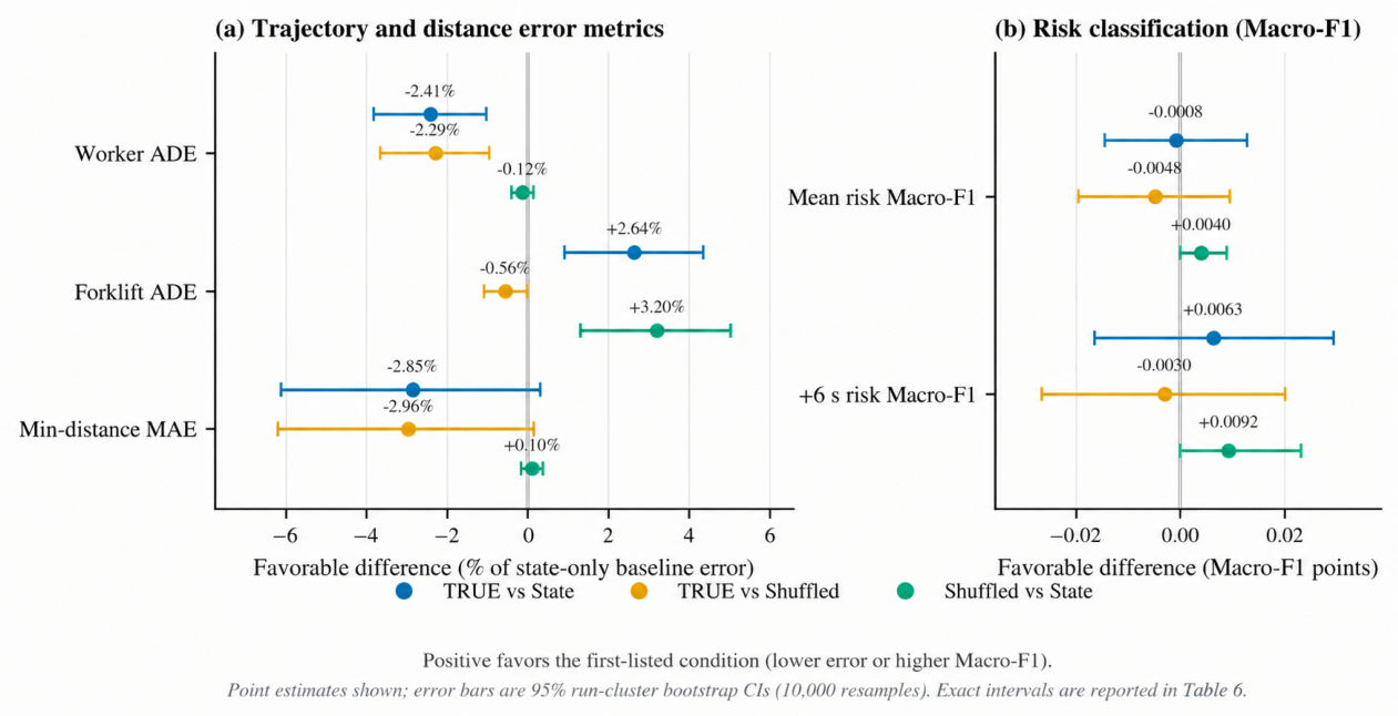
Figure A2.
Performance across the 10 strict shuffled-latent robustness runs. Every permutation prohibits identity
and same-run pairings. The aligned condition is shown as the reference line.
Figure A2.
Performance across the 10 strict shuffled-latent robustness runs. Every permutation prohibits identity
and same-run pairings. The aligned condition is shown as the reference line.
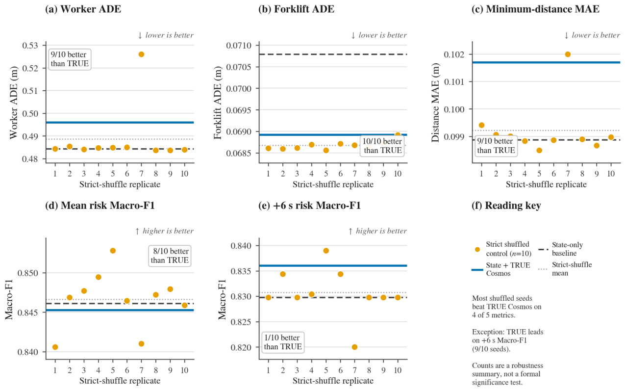
Table A4.
Aggregate results from the earlier Wan development experiments. Lower is better for all metrics. The matched state baseline is shared by the direct-fusion and residual-fusion comparisons.
Table A4.
Aggregate results from the earlier Wan development experiments. Lower is better for all metrics. The matched state baseline is shared by the direct-fusion and residual-fusion comparisons.
| Fusion | Configuration | Worker ADE | Forklift ADE | Dist. MAE |
|---|---|---|---|---|
| Baseline | State-only | 0.425627 | 0.048393 | 0.064016 |
| Direct | TRUE Wan | 0.692429 | 0.075632 | 0.110029 |
| Direct | SHUFFLED Wan | 0.587507 | 0.071234 | 0.111591 |
| Residual | TRUE Wan | 0.420702 | 0.047032 | 0.063245 |
| Residual | SHUFFLED Wan | 0.413694 | 0.046447 | 0.065249 |
References
- Teizer, J.; Allread, B.S.; Fullerton, C.E.; Hinze, J. Autonomous Pro-Active Real-Time Construction Worker and Equipment Operator Proximity Safety Alert System. Autom. Constr. 2010, 19, 630–640. [Google Scholar] [CrossRef]
- Bostelman, R.V.; Shackleford, W.P. Advanced Sensing Towards Improved Forklift Safety. In Proceedings of the Performance Metrics for Intelligent Systems Workshop (PerMIS ’10), Baltimore, MD, USA, 2010. [Google Scholar] [CrossRef]
- Kim, H.; Kim, T.; Jo, W.; Kim, J.; Shin, J.; Han, D.; Hwang, Y.; Choi, Y. Multispectral Benchmark Dataset and Baseline for Forklift Collision Avoidance. Sensors 2022, 22, 7953. [Google Scholar] [CrossRef] [PubMed]
- Lee, H.; Cho, H.; Noh, B.; Yeo, H. NAVIBox: Real-Time Vehicle–Pedestrian Risk Prediction System in an Edge Vision Environment. Electronics 2023, 12, 4311. [Google Scholar] [CrossRef]
- Liu, Y.; Jiang, B.; Xu, Z.; Chen, Z. Collision Warning Method for Workshops Based on Dynamic Target Trajectory Prediction. Proceedings of the Institution of Mechanical Engineers, Part C: Journal of Mechanical Engineering Science 2026, 240, 2343–2358. [Google Scholar] [CrossRef]
- Alahi, A.; Goel, K.; Ramanathan, V.; Robicquet, A.; Fei-Fei, L.; Savarese, S. Social LSTM: Human Trajectory Prediction in Crowded Spaces. In Proceedings of the IEEE Conference on Computer Vision and Pattern Recognition (CVPR), 2016; pp. 961–971. [Google Scholar] [CrossRef]
- Gupta, A.; Johnson, J.; Fei-Fei, L.; Savarese, S.; Alahi, A. Social GAN: Socially Acceptable Trajectories with Generative Adversarial Networks. In Proceedings of the IEEE Conference on Computer Vision and Pattern Recognition (CVPR), 2018; pp. 2255–2264. [Google Scholar] [CrossRef]
- Salzmann, T.; Ivanovic, B.; Chakravarty, P.; Pavone, M. Trajectron++: Dynamically-Feasible Trajectory Forecasting with Heterogeneous Data. In Proceedings of the European Conference on Computer Vision (ECCV), 2020; pp. 683–700. [Google Scholar] [CrossRef]
- Mangalam, K.; Girase, H.; Agarwal, S.; Lee, K.H.; Adeli, E.; Malik, J.; Gaidon, A. It Is Not the Journey But the Destination: Endpoint Conditioned Trajectory Prediction. In Proceedings of the European Conference on Computer Vision (ECCV), 2020; pp. 759–776. [Google Scholar] [CrossRef]
- Mangalam, K.; An, Y.; Girase, H.; Malik, J. From Goals, Waypoints & Paths to Long Term Human Trajectory Forecasting. In Proceedings of the IEEE/CVF International Conference on Computer Vision (ICCV), 2021; pp. 15233–15242. [Google Scholar] [CrossRef]
- Yuan, Y.; Weng, X.; Ou, Y.; Kitani, K.M. AgentFormer: Agent-Aware Transformers for Socio-Temporal Multi-Agent Forecasting. In Proceedings of the IEEE/CVF International Conference on Computer Vision (ICCV), 2021; pp. 9813–9823. [Google Scholar] [CrossRef]
- Zhou, Z.; Ye, L.; Wang, J.; Wu, K.; Lu, K. HiVT: Hierarchical Vector Transformer for Multi-Agent Motion Prediction. In Proceedings of the IEEE/CVF Conference on Computer Vision and Pattern Recognition (CVPR), 2022; pp. 8823–8833. [Google Scholar] [CrossRef]
- Shi, S.; Jiang, L.; Dai, D.; Schiele, B. Motion Transformer with Global Intention Localization and Local Movement Refinement. Adv. Neural Inf. Process. Syst. 2022, 35, 6531–6543. [Google Scholar] [CrossRef]
- Nayakanti, N.; Al-Rfou, R.; Zhou, A.; Goel, K.; Refaat, K.S.; Sapp, B. Wayformer: Motion Forecasting via Simple & Efficient Attention Networks. In Proceedings of the 2023 IEEE International Conference on Robotics and Automation (ICRA), 2023; pp. 2980–2987. [Google Scholar] [CrossRef]
- Zhou, Z.; Wang, J.; Li, Y.H.; Huang, Y.K. Query-Centric Trajectory Prediction. In Proceedings of the IEEE/CVF Conference on Computer Vision and Pattern Recognition (CVPR), 2023; pp. 17863–17873. [Google Scholar] [CrossRef]
- Hu, A.; Russell, L.; Yeo, H.; Murez, Z.; Fedoseev, G.; Kendall, A.; Shotton, J.; Corrado, G. GAIA-1: A Generative World Model for Autonomous Driving. arXiv 2023, arXiv:2309.17080. [Google Scholar] [CrossRef]
- Wang, Y.; He, J.; Fan, L.; Li, H.; Chen, Y.; Zhang, Z. Driving into the Future: Multiview Visual Forecasting and Planning with World Model for Autonomous Driving. In Proceedings of the IEEE/CVF Conference on Computer Vision and Pattern Recognition (CVPR), 2024; pp. 14749–14759. [Google Scholar] [CrossRef]
- Min, C.; Zhao, D.; Xiao, L.; Zhao, J.; Xu, X.; Zhu, Z.; Jin, L.; Li, J.; Guo, Y.; Xing, J.; et al. DriveWorld: 4D Pre-trained Scene Understanding via World Models for Autonomous Driving. In Proceedings of the IEEE/CVF Conference on Computer Vision and Pattern Recognition (CVPR), 2024; pp. 15522–15533. [Google Scholar] [CrossRef]
- Bardes, A.; Garrido, Q.; Ponce, J.; Chen, X.; Rabbat, M.; LeCun, Y.; Assran, M.; Ballas, N. Revisiting Feature Prediction for Learning Visual Representations from Video. arXiv 2024, arXiv:2404.08471. [Google Scholar] [CrossRef]
- Yosinski, J.; Clune, J.; Bengio, Y.; Lipson, H. How Transferable Are Features in Deep Neural Networks? Proc. Adv. Neural Inf. Process. Syst. (NeurIPS) 2014, Vol. 27, 3320–3328. [Google Scholar]
- NVIDIA. World Simulation with Video Foundation Models for Physical AI. arXiv 2025, arXiv:2511.00062. [Google Scholar] [CrossRef]
- Dadhich, N. PhysicalAI SDG-Warehouse: A Synthetic Multi-View Video Dataset of Industrial-Safety Events. NVIDIA. 2026. Available online: https://huggingface.co/datasets/nvidia/PhysicalAI-WorldModel-Synthetic-Warehouse-Operations-Scenes (accessed on 4 September 2026).
- Mohamed, A.; Qian, K.; Elhoseiny, M.; Claudel, C. Social-STGCNN: A Social Spatio-Temporal Graph Convolutional Neural Network for Human Trajectory Prediction. In Proceedings of the IEEE/CVF Conference on Computer Vision and Pattern Recognition (CVPR), 2020; pp. 14424–14432. [Google Scholar] [CrossRef]
- Yu, C.; Ma, X.; Ren, J.; Zhao, H.; Yi, S. Spatio-Temporal Graph Transformer Networks for Pedestrian Trajectory Prediction. In Proceedings of the European Conference on Computer Vision (ECCV), 2020; pp. 507–523. [Google Scholar] [CrossRef]
- Qiu, Y.; Liu, Y. Intent-Aware Spatiotemporal Risk Field for Multi-AGV Path Planning with Heterogeneous Dynamic Obstacles. J. King Saud Univ. Comput. Inf. Sci. 2026, 38, 570. [Google Scholar] [CrossRef]
- Assran, M.; Bardes, A.; Fan, D.; Garrido, Q.; Howes, R.; Komeili, M.; Muckley, M.; Rizvi, A.; Roberts, C.; Sinha, K.; et al. V-JEPA 2: Self-Supervised Video Models Enable Understanding, Prediction and Planning. arXiv 2025, arXiv:2506.09985. [Google Scholar] [CrossRef]
- Kornblith, S.; Shlens, J.; Le, Q.V. Do Better ImageNet Models Transfer Better? In Proceedings of the IEEE/CVF Conference on Computer Vision and Pattern Recognition (CVPR), 2019; pp. 2661–2671. [Google Scholar] [CrossRef]
- Ericsson, L.; Gouk, H.; Hospedales, T.M. How Well Do Self-Supervised Models Transfer? In Proceedings of the IEEE/CVF Conference on Computer Vision and Pattern Recognition (CVPR), 2021; pp. 5414–5423. [Google Scholar] [CrossRef]
- NVIDIA. Cosmos 3: Omnimodal World Models for Physical AI. arXiv 2026, arXiv:2606.02800. [Google Scholar] [CrossRef]
- Schöller, C.; Aravantinos, V.; Lay, F.; Knoll, A. What the Constant Velocity Model Can Teach Us About Pedestrian Motion Prediction. IEEE Robot. Autom. Lett. 2020, 5, 1696–1703. [Google Scholar] [CrossRef]
- Maes, L.; Le Lidec, Q.; Scieur, D.; LeCun, Y.; Balestriero, R. LeWorldModel: Stable End-to-End Joint-Embedding Predictive Architecture from Pixels. arXiv 2026, arXiv:2603.19312. [Google Scholar] [CrossRef]
- Li, L.; Wang, S.; Qiu, L.; Xiong, M.; Liu, Q. World Model Control by Trajectory Reachability Metrics. arXiv 2026, arXiv:2605.22164. [Google Scholar] [CrossRef]
- Li, W.; Li, G.; Maeda, K.; Ogawa, T.; Haseyama, M. Predictive but Not Plannable: RC-aux for Latent World Models. arXiv 2026, arXiv:2605.07278. [Google Scholar] [CrossRef]
- Kim, M.J.; Gao, Y.; Lin, T.Y.; Lin, Y.C.; Ge, Y.; Lam, G.; Liang, P.; Song, S.; Liu, M.Y.; Finn, C.; et al. Cosmos Policy: Fine-Tuning Video Models for Visuomotor Control and Planning. In Proceedings of the International Conference on Learning Representations (ICLR), 2026. [Google Scholar] [CrossRef]
- Wang, A.; Ai, B.; Wen, B.; Mao, C.; Xie, C.W.; Chen, D.; Yu, F.; Zhao, H.; Yang, J.; Zeng, J.; et al. Wan: Open and Advanced Large-Scale Video Generative Models. arXiv 2025, arXiv:2503.20314. [Google Scholar] [CrossRef]
Figure 1.
Conceptual formulation of long-horizon forklift–worker risk forecasting. The model observes a 20-step kinematic history sampled at 10 Hz and predicts worker and forklift positions at horizons from to s. Safety risk is derived from the cumulative minimum worker–forklift separation between the prediction anchor and each forecast horizon, allowing a close approach occurring before the endpoint to be retained. HIGH, WARNING, and SAFE denote the study-specific operational risk bands used in this work rather than regulatory safety limits.
Figure 1.
Conceptual formulation of long-horizon forklift–worker risk forecasting. The model observes a 20-step kinematic history sampled at 10 Hz and predicts worker and forklift positions at horizons from to s. Safety risk is derived from the cumulative minimum worker–forklift separation between the prediction anchor and each forecast horizon, allowing a close approach occurring before the endpoint to be retained. HIGH, WARNING, and SAFE denote the study-specific operational risk bands used in this work rather than regulatory safety limits.
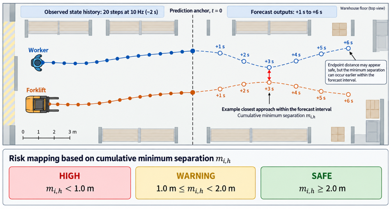
Figure 2.
Overall forecasting workflow. The primary state-based path maps the kinematic history to joint worker–forklift trajectory and cumulative minimum-separation predictions, from which the operational risk class is derived. The frozen Cosmos Predict2.5 Video2World branch is evaluated as an additional candidate representation that contributes a learned residual correction and is not an always-active component of the primary state-based forecasting path.
Figure 2.
Overall forecasting workflow. The primary state-based path maps the kinematic history to joint worker–forklift trajectory and cumulative minimum-separation predictions, from which the operational risk class is derived. The frozen Cosmos Predict2.5 Video2World branch is evaluated as an additional candidate representation that contributes a learned residual correction and is not an always-active component of the primary state-based forecasting path.
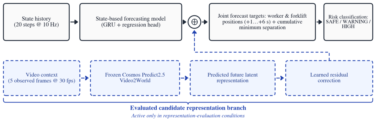
Figure 3.
Controlled A/B/C/D experimental protocol. Condition A establishes the matched state-only reference model. Conditions B and C reuse the trained Condition-A state predictor in frozen form and train the same zero-initialized Conv3D residual architecture; their principal difference is whether the Cosmos predictive latent is correctly aligned with the current sample or permuted within the corresponding data split. Condition D removes the kinematic state branch and predicts directly from the aligned Cosmos latent using the same latent-branch architecture as the B/C residual branch, without implying shared weights.
Figure 3.
Controlled A/B/C/D experimental protocol. Condition A establishes the matched state-only reference model. Conditions B and C reuse the trained Condition-A state predictor in frozen form and train the same zero-initialized Conv3D residual architecture; their principal difference is whether the Cosmos predictive latent is correctly aligned with the current sample or permuted within the corresponding data split. Condition D removes the kinematic state branch and predicts directly from the aligned Cosmos latent using the same latent-branch architecture as the B/C residual branch, without implying shared weights.
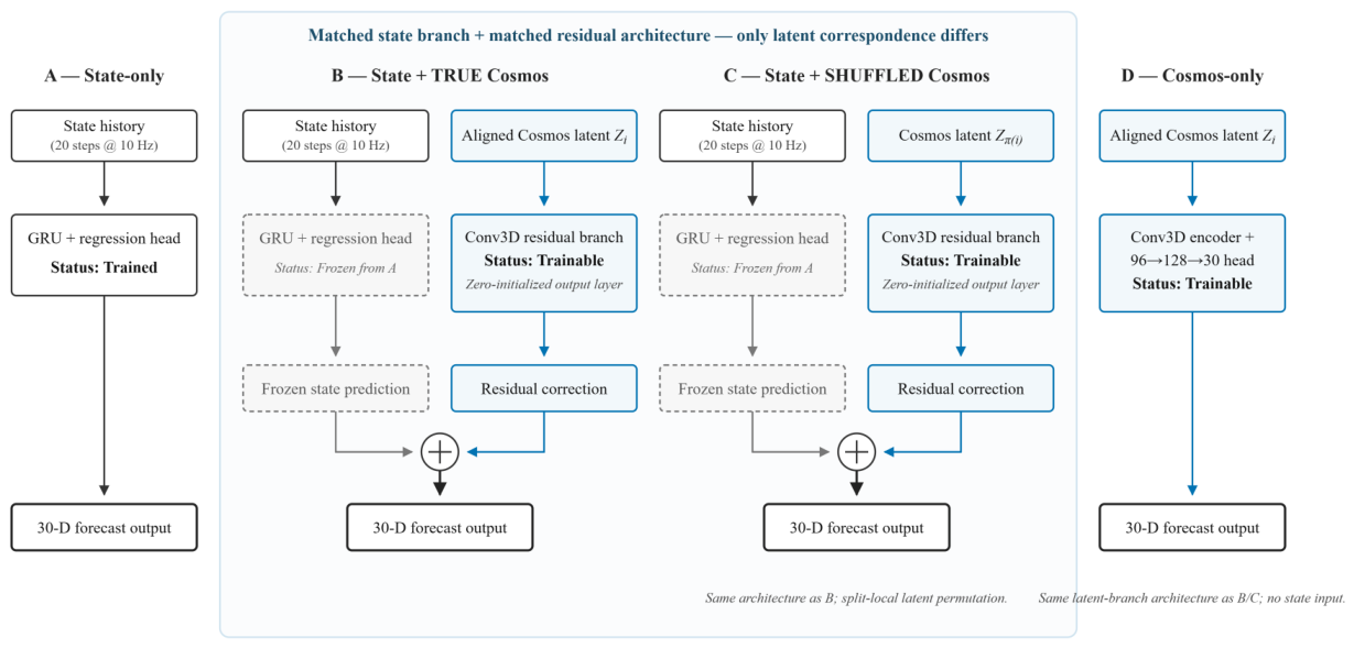
Figure 4.
Forklift target-distribution, motion, and forecasting-error trends across the evaluated forecast horizons.
Panel (a) shows the horizon-specific RMS spread of the ground-truth forklift positions, the mean forklift displacement
during the preceding one-second interval, and the fraction of samples moving less than 0.10m during
that interval. Panel (b) shows the corresponding state-only forklift displacement error. The concurrent decrease
in target spread, preceding motion, and forecasting error is interpreted as an association with the increasingly
concentrated, low-motion late-horizon target regime rather than as evidence of a causal mechanism. Exact
diagnostic values are reported in Table A3, and the state-only forklift errors are reported in Table 7.
Figure 4.
Forklift target-distribution, motion, and forecasting-error trends across the evaluated forecast horizons.
Panel (a) shows the horizon-specific RMS spread of the ground-truth forklift positions, the mean forklift displacement
during the preceding one-second interval, and the fraction of samples moving less than 0.10m during
that interval. Panel (b) shows the corresponding state-only forklift displacement error. The concurrent decrease
in target spread, preceding motion, and forecasting error is interpreted as an association with the increasingly
concentrated, low-motion late-horizon target regime rather than as evidence of a causal mechanism. Exact
diagnostic values are reported in Table A3, and the state-only forklift errors are reported in Table 7.
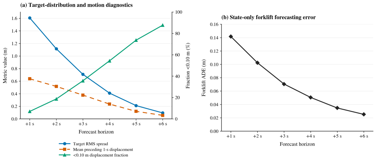
Table 1.
Comparison with closely related industrial human–vehicle safety studies. Entries summarize each study’s formulation; the table is not a numerical ranking.
Table 1.
Comparison with closely related industrial human–vehicle safety studies. Entries summarize each study’s formulation; the table is not a numerical ranking.
| Study | Setting | Predicted quantity | Agents forecast | Risk definition |
|---|---|---|---|---|
| Kim et al. [3] | Intralogistics forklift; real RGB and thermal | Pedestrian detection and frame-level 3-D distance | – | Distance-based hazard and warning regions |
| NAVIBox [4] | Road vehicle–pedestrian; real edge deployment | Refined future trajectories | Vehicles and pedestrians | Predicted interaction risk |
| Liu et al. [5] | Workshop with unmanned forklifts | Pedestrian trajectory and human–machine distance | Pedestrians | Graded collision warning |
| Qiu and Liu [25] | Warehouse multi-AGV planning | Trajectories of external obstacles (forklifts, personnel) | Dynamic obstacles | Spatio-temporal risk field for planning |
| Ours | Synthetic warehouse; exact metric state | Joint positions at to s and cumulative minimum separation | Worker and forklift | HIGH, WARNING, or SAFE from cumulative minimum separation |
Table 2.
Dataset construction summary prior to rolling-window generation.
| Stage | Count |
|---|---|
| Near-miss runs in dataset metadata | 13,410 |
| Runs with a ceiling_00 RGB clip | 1,619 |
| Parsed near-miss annotation runs | 1,542 |
| Dynamically valid expansion runs | 878 |
| Frozen-position runs excluded | 659 |
| Insufficient-frame runs excluded | 5 |
| Previously verified dynamic runs added | 17 |
| Master dynamic runs | 895 |
| Expansion runs supporting 2 s → 6 s | 837 |
| Final long-horizon eligible runs | 854 |
Table 3.
Final long-horizon rolling dataset.
| Partition | Runs | Rolling samples |
|---|---|---|
| Training | 597 | 6,428 |
| Validation | 128 | 1,371 |
| Test | 129 | 1,390 |
| Total | 854 | 9,189 |
Table 4.
Aggregate performance of the four controlled conditions on the 300-sample Cosmos test partition. Lower is better for trajectory and distance errors; higher is better for risk metrics. Boldface denotes the best result in each column.
Table 4.
Aggregate performance of the four controlled conditions on the 300-sample Cosmos test partition. Lower is better for trajectory and distance errors; higher is better for risk metrics. Boldface denotes the best result in each column.
| Configuration | Worker ADE |
Forklift ADE |
Min-dist. MAE |
Mean Bal. Acc. |
Mean Macro-F1 |
s Macro-F1 |
|---|---|---|---|---|---|---|
| A: State-only | 0.4843 | 0.0708 | 0.0989 | 0.8366 | 0.8461 | 0.8298 |
| B: State + TRUE Cosmos | 0.4960 | 0.0689 | 0.1017 | 0.8356 | 0.8453 | 0.8360 |
| C: State + SHUFFLED Cosmos | 0.4849 | 0.0685 | 0.0988 | 0.8407 | 0.8501 | 0.8390 |
| D: Cosmos-only | 2.0692 | 0.4685 | 0.5049 | 0.3408 | 0.2704 | 0.2526 |
Table 5.
Paired run-level cluster-bootstrap differences on the controlled test partition. Values are reported as point difference [95% percentile CI]; trajectory and distance differences are given in millimeters. Positive values favor the first-listed condition under the metric-specific direction defined in the text.
Table 5.
Paired run-level cluster-bootstrap differences on the controlled test partition. Values are reported as point difference [95% percentile CI]; trajectory and distance differences are given in millimeters. Positive values favor the first-listed condition under the metric-specific direction defined in the text.
| Metric | B vs. A | B vs. C | C vs. A |
|---|---|---|---|
| Worker ADE (mm) | [, ] | [, ] | [, ] |
| Forklift ADE (mm) | [, ] | [, ] | [, ] |
| Min-distance MAE (mm) | [, ] | [, ] | [, ] |
| Mean risk Macro-F1 | [, ] | [, ] | [, ] |
| s risk Macro-F1 | [, ] | [, ] | [, ] |
Table 6.
Horizon-wise results for worker displacement error, cumulative minimum-distance MAE, and risk Macro-F1 in the main controlled experiment. Lower is better for displacement and distance errors; higher is better for Macro-F1.
Table 6.
Horizon-wise results for worker displacement error, cumulative minimum-distance MAE, and risk Macro-F1 in the main controlled experiment. Lower is better for displacement and distance errors; higher is better for Macro-F1.
| Metric | Configuration | s | s | s | s | s | s |
|---|---|---|---|---|---|---|---|
| Worker error (m) | State-only | 0.1980 | 0.3632 | 0.5048 | 0.5742 | 0.6164 | 0.6493 |
| State + TRUE Cosmos | 0.1970 | 0.3623 | 0.5129 | 0.5864 | 0.6371 | 0.6802 | |
| State + SHUFFLED Cosmos | 0.1982 | 0.3631 | 0.5058 | 0.5740 | 0.6177 | 0.6507 | |
| Cosmos-only | 1.2202 | 1.6525 | 2.0467 | 2.3257 | 2.5192 | 2.6508 | |
| Distance MAE (m) | State-only | 0.0799 | 0.0943 | 0.1042 | 0.1022 | 0.1051 | 0.1076 |
| State + TRUE Cosmos | 0.0800 | 0.0949 | 0.1064 | 0.1069 | 0.1106 | 0.1114 | |
| State + SHUFFLED Cosmos | 0.0800 | 0.0939 | 0.1040 | 0.1020 | 0.1051 | 0.1076 | |
| Cosmos-only | 0.5759 | 0.5294 | 0.4917 | 0.4775 | 0.4754 | 0.4796 | |
| Risk Macro-F1 | State-only | 0.8888 | 0.8330 | 0.8215 | 0.8489 | 0.8547 | 0.8298 |
| State + TRUE Cosmos | 0.8937 | 0.8403 | 0.8270 | 0.8303 | 0.8444 | 0.8360 | |
| State + SHUFFLED Cosmos | 0.8888 | 0.8426 | 0.8217 | 0.8537 | 0.8547 | 0.8390 | |
| Cosmos-only | 0.3392 | 0.2670 | 0.2534 | 0.2560 | 0.2543 | 0.2526 |
Table 7.
Forklift displacement error (m) by forecast horizon for the main controlled experiment.
| Configuration | s | s | s | s | s | s | Mean |
|---|---|---|---|---|---|---|---|
| State-only | 0.1417 | 0.1024 | 0.0705 | 0.0505 | 0.0347 | 0.0251 | 0.0708 |
| State + TRUE Cosmos | 0.1345 | 0.0986 | 0.0692 | 0.0504 | 0.0354 | 0.0254 | 0.0689 |
| State + SHUFFLED Cosmos | 0.1329 | 0.0985 | 0.0693 | 0.0504 | 0.0349 | 0.0251 | 0.0685 |
| Cosmos-only | 1.2844 | 0.7918 | 0.4191 | 0.1873 | 0.0817 | 0.0470 | 0.4685 |
Table 8.
Safety-specific diagnostics at the s horizon. HIGH→WARNING and HIGH→SAFE denote the numbers of ground-truth HIGH samples assigned to those lower-risk classes. There are 70 ground-truth HIGH samples at this horizon.
Table 8.
Safety-specific diagnostics at the s horizon. HIGH→WARNING and HIGH→SAFE denote the numbers of ground-truth HIGH samples assigned to those lower-risk classes. There are 70 ground-truth HIGH samples at this horizon.
| Configuration | HIGH precision | HIGH recall | WARNING recall | HIGH→WARNING | HIGH→SAFE |
|---|---|---|---|---|---|
| State-only | 0.8837 | 0.5429 | 0.9344 | 32 | 0 |
| State + TRUE Cosmos | 0.8696 | 0.5714 | 0.9290 | 30 | 0 |
| State + SHUFFLED Cosmos | 0.8889 | 0.5714 | 0.9344 | 30 | 0 |
| Cosmos-only | 0.0000 | 0.0000 | 1.0000 | 70 | 0 |
Table 9.
Strict multi-permutation shuffled-latent robustness analysis. Each shuffled control prohibits both identity and same-run pairings. “Better than TRUE” reports the number of the 10 shuffled runs outperforming the aligned Condition B under the corresponding metric direction.
Table 9.
Strict multi-permutation shuffled-latent robustness analysis. Each shuffled control prohibits both identity and same-run pairings. “Better than TRUE” reports the number of the 10 shuffled runs outperforming the aligned Condition B under the corresponding metric direction.
| Metric | TRUE Cosmos | Strict shuffle mean | Strict shuffle range | Better than TRUE |
|---|---|---|---|---|
| Worker ADE (m) | 0.495994 | 0.488564 | 0.483618–0.526076 | 9/10 |
| Forklift ADE (m) | 0.068919 | 0.068674 | 0.068558–0.068914 | 10/10 |
| Min-distance MAE (m) | 0.101697 | 0.099222 | 0.098493–0.102000 | 9/10 |
| Mean risk Macro-F1 | 0.845282 | 0.846603 | 0.840617–0.852809 | 8/10 |
| s risk Macro-F1 | 0.836026 | 0.830702 | 0.820039–0.838990 | 1/10 |
Table 10.
Matched state, Cosmos-only, and non-learned reference baselines on the controlled test partition. Worker FDE denotes displacement error at s. Onset metrics are defined in Section 6.4. Lower is better for error and false-alarm metrics; higher is better for Macro-F1 and recall.
Table 10.
Matched state, Cosmos-only, and non-learned reference baselines on the controlled test partition. Worker FDE denotes displacement error at s. Onset metrics are defined in Section 6.4. Lower is better for error and false-alarm metrics; higher is better for Macro-F1 and recall.
| Configuration | Worker ADE |
Worker FDE |
Forklift ADE |
Min-dist. MAE |
Mean Macro-F1 |
s Macro-F1 |
s HIGH recall |
Onset recall |
Onset false alarm |
|---|---|---|---|---|---|---|---|---|---|
| State-only (A) | 0.4843 | 0.6493 | 0.0708 | 0.0989 | 0.8461 | 0.8298 | 0.5429 | 0.5616 | 0.0224 |
| Cosmos-only (D) | 2.0692 | 2.6508 | 0.4685 | 0.5049 | 0.2704 | 0.2526 | 0.0000 | 0.0000 | 0.0000 |
| Train-mean | 2.0445 | 2.6273 | 0.4789 | 0.5146 | 0.2439 | 0.2526 | 0.0000 | 0.0000 | 0.0000 |
| Persistence | 1.7646 | 2.6656 | 1.4556 | 0.7184 | 0.4322 | 0.3551 | 0.1143 | 0.0000 | 0.0000 |
| Constant velocity (anchor) | 2.1676 | 3.8440 | 0.9876 | 0.4500 | 0.6440 | 0.6067 | 0.6714 | 0.5399 | 0.2710 |
| Causal constant velocity | 1.9968 | 3.3304 | 1.0328 | 0.4699 | 0.6716 | 0.6389 | 0.7143 | 0.5942 | 0.3103 |
| Damped constant velocity | 1.4216 | 2.2195 | 0.5842 | 0.3111 | 0.6815 | 0.6472 | 0.5714 | 0.4312 | 0.1714 |
Table 11.
State-only predictor retrained using the original and strictly causal velocity features. Values are mean ± standard deviation over three training seeds. These retraining results are used as a sensitivity analysis and are distinct from the locked Condition-A checkpoint.
Table 11.
State-only predictor retrained using the original and strictly causal velocity features. Values are mean ± standard deviation over three training seeds. These retraining results are used as a sensitivity analysis and are distinct from the locked Condition-A checkpoint.
| Inputs | Worker ADE | s worker | Forklift ADE | Min-dist. MAE | Mean Macro-F1 | s Macro-F1 |
|---|---|---|---|---|---|---|
| Original | ||||||
| Causal | ||||||
| Causal − original |
Table 12.
Robustness of the aligned-versus-shuffled comparison. (a) Risk threshold sensitivity: s class counts (HIGH/WARNING/SAFE), paired run-level bootstrap difference B−C (positive favors aligned) with 95% interval, and the number of the ten strict shuffles that outperform the aligned condition. (b) Alternative latent probes on the frozen Condition-A predictor: number of the ten strict shuffles outperforming the aligned latent for each metric.
Table 12.
Robustness of the aligned-versus-shuffled comparison. (a) Risk threshold sensitivity: s class counts (HIGH/WARNING/SAFE), paired run-level bootstrap difference B−C (positive favors aligned) with 95% interval, and the number of the ten strict shuffles that outperform the aligned condition. (b) Alternative latent probes on the frozen Condition-A predictor: number of the ten strict shuffles outperforming the aligned latent for each metric.
| (a) Risk thresholds | |||||
|---|---|---|---|---|---|
| HIGH / WARNING bands (m) | s counts | B−C mean Macro-F1 | B−C s Macro-F1 | Strict > aligned (mean / s) | |
| 1.0 / 2.0 (main) | 70/183/47 | [, ] | [, ] | 8/10 / 1/10 | |
| 0.75 / 1.5 | 2/163/135 | [, ] | [, ] | 0/10 / 0/10 | |
| 1.25 / 2.5 | 155/125/20 | [, ] | [, ] | 0/10 / 0/10 | |
| 1.5 / 3.0 | 165/131/4 | [, ] | [, ] | 10/10 / 9/10 | |
| (b) Latent probe on the frozen GRU (strict shuffles outperforming aligned, of 10) | |||||
| Probe | Worker ADE | Forklift ADE | Min-dist. MAE | Mean Macro-F1 | s Macro-F1 |
| Conv3D, global pooling (Condition B) | 9/10 | 10/10 | 9/10 | 8/10 | 1/10 |
| Ridge, global pooling | 9/10 | 8/10 | 1/10 | 3/10 | 0/10 |
| Ridge, pooling | 9/10 | 0/10 | 0/10 | 6/10 | 1/10 |
| Ridge, pooling | 9/10 | 0/10 | 2/10 | 0/10 | 2/10 |
| Attention, 720 tokens | 10/10 | 9/10 | 0/10 | 6/10 | 6/10 |
Table 13.
Summary of threats to validity and how they are addressed.
| Threat | Possible effect on the conclusions | How it is addressed |
|---|---|---|
| Synthetic data with exact metric state | Absolute errors and risk performance may not transfer to real warehouses | Results are framed as forecasting under exact metric state; real-data validation is left to future work |
| Short visual context and reduced inference setting | Motion and fine spatial cues may be under-represented in the latent | The conditioning constraint is explained; Wan2.2 latents covering the full 2 s window show the same pattern |
| Choice of latent probe | Information may be present but inaccessible to the probe | Conv3D, ridge probes at three pooling resolutions, and a token-preserving attention probe give the same aligned-versus-shuffled pattern |
| No task-specific adaptation | An adapted world model might add information | The conclusion is restricted to the frozen backbone |
| One-step velocity look-ahead | The state baseline could be inflated | Causal retraining changes results by less than seed-to-seed variability |
| Test size (300 samples, 129 runs) | Small effects may be missed | Run-level cluster bootstrap; the intervals bound any aligned benefit in mean Macro-F1 below 0.01 |
| Finite shuffle sample and training variability | Shuffle-specific effects could mask or mimic a benefit | Ten strict permutations; the paired frozen-predictor design removes state-predictor variability from the B–C comparison |
| Single state architecture | Conclusions could depend on the GRU | The B–C test is paired on the same frozen predictor; a stronger predictor would leave less residual to explain |
| Study-specific risk thresholds | Risk-level results could change with other bands | Four threshold sets and threshold-free minimum-distance MAE are reported |
Disclaimer/Publisher’s Note: The statements, opinions and data contained in all publications are solely those of the individual author(s) and contributor(s) and not of MDPI and/or the editor(s). MDPI and/or the editor(s) disclaim responsibility for any injury to people or property resulting from any ideas, methods, instructions or products referred to in the content. |
© 2026 by the authors. Licensee MDPI, Basel, Switzerland. This article is an open access article distributed under the terms and conditions of the Creative Commons Attribution (CC BY) license (http://creativecommons.org/licenses/by/4.0/).
Copyright: This open access article is published under a Creative Commons CC BY 4.0 license, which permit the free download, distribution, and reuse, provided that the author and preprint are cited in any reuse.