

Submitted:
19 October 2026
Posted:
21 October 2026
You are already at the latest version
Abstract
Discrete global grid systems (DGGSs) organize geographic data as indexed cells whose neighborhoods support spatial queries. We study exact halo construction on a triangular DGGS and its use in buffer coverage. Rather than store refined connectivity, the architecture reconstructs adjacency using compact integer triangular indices and an Atlas of Connectivity Maps. A graphics processing unit (GPU) resident hash frontier admits each new cell once. Probe reduction and reusable output staging reduce repeated work and delivery costs. Measurements through level 28 compare serial and twenty thread central processing unit (CPU) baselines using flat hash tables, on an Intel Core i7 12700K and NVIDIA RTX 4070. The largest halo contains 10.8 million cells and reaches page locked (pinned) host memory in 13.3 ms; its returned container copy is measured separately. Small queries favor CPU execution. Independent mesh references validate Pentakis adjacency, while the performance runs check cumulative output agreement. A stopping argument connects complete rings to conservative distance coverage, conditional on valid source and distance bounds. A separate World Geodetic System 1984 boundary buffer study includes source covering and distance filtering; CPU execution is faster in all seven cases. Numerical tests do not certify floating point distance bounds.
Keywords:
discrete global grid system
; triangular spherical mesh
; spatial neighborhood
; Atlas of Connectivity Maps
; halo query
; hierarchical indexing
; graphics processing unit
algorithmAlgorithmAlgorithms algorithmAlgorithmAlgorithms
1. Introduction
Discrete global grid systems (DGGSs) provide a geospatial platform [1,2]. Systems such as H3 [3], S2 [4], and rHEALPix [5], together with research systems [6,7,8], partition the Earth into hierarchies of indexed cells at multiple resolutions. These cell indices support aggregation, joins, and neighborhood queries across applications such as urban analytics, Earth observation, climate modeling, and logistics.
Spatial proximity is an important operation in these applications. Buffering a road network, identifying facilities within a service radius, and retrieving parcels near a flood zone ask a common question: given a source region, what lies within a specified distance? In a DGGS, proximity also has a discrete form. Starting from cells covering the source, one expands through cells that share an edge and counts the adjacency steps. This count is the topological distance. Cell indices make these steps suitable for parallel execution because adjacent cells can be constructed without repeatedly measuring geographic distances. Two practical questions follow: how can topological rings be computed efficiently at fine resolutions, and how can their expansion support complete coverage of a requested distance in meters?
Our computational workload begins with the stored cell indices needed by the first question. A halo query constructs the cells reached after one, two, and up to a requested number of edge adjacency steps. Such queries support repeated neighborhood access to data already assigned to a DGGS, for example when changing the neighborhood depth around a fixed indexed feature. Their cost is distinct from assigning a new geographic dataset to cells or evaluating a buffer in meters. The measured acceleration concerns this indexed halo operation. The second question is addressed by a separate boundary buffer study that adds source covering and geometric distance tests around the same halo component.
A concrete example connects these questions. Consider all locations within 1 km of the complete boundary of Nose Hill Park in Calgary. The source is the boundary curve, not the filled park, so the requested region extends to both sides of that curve, as shown in Figure 1(a). Cells covering the complete curve form the seed set P. Starting from these cells, the halo query repeatedly finds cells that share an edge with the current ring. Cells first reached after one step form the halo ring; cells first reached after two steps form , and so on, up to the requested hop depth K. Figure 1(b) shows the first three rings, and Section 3.1 gives the formal definition. The same boundary request is used in the measured ellipsoidal experiment.
A ring count alone does not establish that the whole 1 km boundary buffer has been reached. The procedure must first cover the complete source, expand enough rings, and then exclude cells that cannot intersect the requested region. Figure 1(c) illustrates a conservative cover: every required cell is retained, but some additional cells may remain. Geometric subdivision can tighten a distance test for an uncertain cell without changing the cell being returned or the query resolution. Choosing a finer query resolution is a different operation that produces smaller returned cells. The coverage conditions and the numerical limits of filtering are developed in Section 3.5.1 and Section 3.5.2.
The distance request therefore has two connected stages: construct the cells reached by adjacency, then use geometric tests to decide whether expansion is sufficient and which cells to retain. Efficient ring construction is the shared computational foundation. The first computational difficulty is the size of the refined grid. A triangular base mesh, meaning the coarse polyhedron from which cells are refined, contains cells at level r when each of its F faces is repeatedly divided into four child triangles. Fine resolutions therefore produce far more cells than a local query needs. Storing three adjacent cell indices for every refined cell would allocate memory for the whole Earth even when the requested halo covers only a small region. We instead need to construct adjacency only for cells involved in the query.
The second difficulty concerns how each cell is indexed. A hierarchical index records the base mesh face and one child digit for every refinement. This form supports direct access to ancestors and contiguous ranges of descendants [8,10]. Constructing an adjacent cell at the same resolution can instead require decoding and updating the geometric state represented by those digits. Integer coordinates support adjacency through a small number of arithmetic operations, but do not express the refinement sequence as a visible prefix. A halo query therefore benefits from a hierarchical index for storage and hierarchy operations, and a coordinate representation for repeated adjacency calculations.
Parallel expansion introduces the third difficulty. Each triangular cell in the current ring has three edge adjacent cells. Different workers can generate the same adjacent cell, and a generated cell may also belong to the seed set or an earlier ring. The query must reject these repeated discoveries and add every new cell exactly once. The central problem is therefore to construct exact halo rings at fine resolutions while storing query sized state and coordinating parallel discoveries, without storing the complete refined adjacency structure.
We address these three difficulties with connected design choices. First, a dual index architecture uses one index for the query interface and another during expansion. Cells enter and leave the query as a public hierarchical index, which records the base mesh face, refinement sequence, and resolution. Each input is converted once into a compact integer triangular index, which stores the face, two integer coordinates, and the triangle orientation in one 64 bit word. This representation constructs adjacent cells at the shared query resolution through direct arithmetic. Only the completed output is converted back. Section 3.3.3 places this representation in the context of existing coordinate indexes; the performance evaluation compares our execution variants on the same topology.
Second, adjacency is reconstructed rather than stored. Each base mesh face has a chart: a planar coordinate domain used for its triangular subdivision. Fixed integer rules construct adjacent cells that remain in the same chart. For a cell beside a base mesh edge, the Atlas of Connectivity Maps (ACM) records how coordinates continue into the neighboring chart [11]. Each record identifies the destination face, the shared edge, and the ordering of cells along that edge. Deterministic refinement allows the same records to apply at every resolution. Local arithmetic and directed base mesh edge records therefore describe the refined adjacency without storing a record for each refined cell.
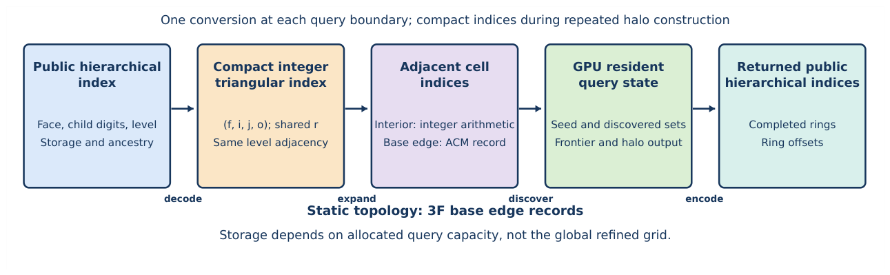
Third, the expansion state remains in graphics processing unit (GPU) memory. This state includes the seed cells, cells already discovered, and the current and next rings. A hash table stores the discovered cell indices. An atomic insertion allows only one worker to register a new index, even if other workers attempt the same insertion simultaneously. The successful worker adds the cell to the next ring; workers that find the index already present do not add it again. This connects duplicate removal directly to ring construction and avoids transferring intermediate rings to the central processing unit (CPU). Figure 5 shows the complete query sequence, while Figure 10 explains the insertion procedure after its data structures have been introduced.
The Pentakis dodecahedron is our primary research base mesh, following the triangular mesh construction studied by Wecker et al. [8]. We choose it to test the atlas on multiple face arrangements, not because of a demonstrated adoption or performance advantage over established DGGS libraries. Its 60 triangular faces include vertices where five faces meet and others where six meet. Testing both arrangements checks movement among different numbers of adjacent faces. At level 28, this mesh contains approximately cells, with a global average area of about square centimeters per cell. The architecture nevertheless stores only its 180 directed base mesh edge records and allocated query state. Within the current six bit face field, the same execution method supports oriented triangular base meshes with at most 64 faces that use the same subdivision. An icosahedron requires 60 directed records and an octahedron requires 24. Their performance must still be evaluated separately under comparable spatial workloads.
We evaluate the architecture by comparing parallel performance, isolating component contributions, measuring complete workflow costs, and testing correctness. Official City of Calgary building, street, and boundary data supply 81 configurations through level 28. On the tested Intel Core i7 12700K and NVIDIA RTX 4070, the GPU implementation is faster than the better of two CPU baselines that store the discovered set in a flat open addressing table (the flat table baselines of Section 3.4.1) in 48 of the 81 configurations; the median ratio over all configurations is , and the 33 configurations won by the CPU return at most 3,000 cells. The largest query constructs 10.8 million halo cells from 100,000 building seed cells in 13.3 ms, measured to page locked (pinned) host memory, compared with 117 ms for the twenty thread flat table. Sections 3.6.4 and 4.1.1 state the timing boundaries, the selection of measurement sessions, and its sensitivity. These ratios compare GPU pinned host readiness with CPU returned container completion; the additional GPU container copy is reported separately. Mapping points to cells, source covering, and rendering are excluded from these times. Independent topology tests exercise every directed base mesh edge and every base mesh vertex of the Pentakis mesh; output agreement checks for the measured configurations are reported separately.
The second stage uses these rings to evaluate the same boundary distance request. It constructs World Geodetic System 1984 (WGS84) buffers using complete source covering, adaptive halo expansion, and curved cell distance tests. In all seven tested buffer configurations, the CPU only variant is faster than the hybrid variant, which runs ring expansion on the GPU and the geometric tests on the CPU, because geometric processing and GPU initialization dominate the total cost. This is distinct from the measured acceleration of the reusable halo component. The implementation retains unresolved cells and states its numerical allowances. No formal correctness proof of the floating point distance implementation is provided; its implementation evidence is numerical validation.
The primary contribution is an execution architecture for exact halo construction from stored indices. The boundary buffer study demonstrates the additional geometric requirements and their present cost. The first stage addresses the cost of large adjacency expansions; the second specifies the additional geometric conditions needed for a distance request. The contributions are:
- Query specific representation and execution. A public hierarchical index serves storage and hierarchy operations; a compact integer triangular index serves repeated adjacency and discovery. Building on established indexing and atlas principles, the architecture reconstructs neighbors from arithmetic and base mesh edge records, without refined connectivity arrays.
- Concurrent exact ring construction. A GPU resident discovered set rejects repeated cells and authorizes exactly one append for every newly admitted cell. Cooperative ring scheduling retains intermediate state on the device. Memory depends on input, hash, and output capacities rather than the global cell count.
- Independent validation. Geometric references that do not consult the runtime atlas check base mesh and refined adjacency. Globally distributed queries exercise all directed base mesh edges and base mesh vertices of the Pentakis mesh, while failure tests require explicit errors instead of incomplete results.
- Measured performance and limits. Serial and multithreaded flat table baselines, a thread count sweep, stage measurements, and controlled mechanism changes identify the workload and delivery conditions that support acceleration. Sensitivity to the measurement session and a local routing check state the limits of those findings.
- Distance coverage conditions. Complete source covering, a whole ring stopping argument, and cell extent bounds connect exact topological expansion to conservative spatial coverage. A separate WGS84 boundary study evaluates the additional geometric work and its numerical limits; CPU execution is faster for its tested complete queries.
The work does not introduce a new projection or replace established DGGS indexing principles. It connects representations suited to repeated adjacency with geometric tests suited to distance requests. After defining exact rings and their spherical interpretation, we explain the indices and execution methods used to construct them. We then add source covering, stopping, and filtering to obtain boundary buffers. The evaluation separates the performance of the halo component from the cost and numerical limitations of the complete query.
2. Background and Related Work
This section introduces the foundations needed to understand the problem and the proposed solution. We first review how a discrete global grid system divides the Earth, identifies its cells, and defines neighborhood operations. We then explain the triangular coordinates and connectivity atlases that make local cell adjacency possible. Finally, we review parallel frontier processing and identify the remaining difficulty: constructing a very large set of newly discovered cells without storing the complete refined topology.
2.1. DGGS Foundations: Domains, Indexing, and Neighborhood Operations
A discrete global grid system (DGGS) divides a spherical or ellipsoidal Earth model into cells at several resolutions. Its projection, refinement, and indexing rules determine how locations are assigned to cells and how those cells are organized [1]. The cell shape and the coarse polyhedron, called the base mesh, strongly influence refinement, distortion, and neighborhood structure. Hexagons provide nearly uniform adjacency, but their fractional refinement does not form a simple congruent subdivision. Quadrilaterals align naturally with raster storage; their distortion depends on the base mesh and projection, with polar distortion arising in some constructions. Triangles are planar primitives that admit a congruent subdivision in which every triangle is replaced by four smaller triangles [6,12]. Prominent triangular base meshes include the octahedron used by the Hierarchical Triangular Mesh [13], the icosahedron used by many geodesic grids [12], and the Disdyakis triacontahedron with 120 triangular faces [7]. We use the Pentakis dodecahedron with 60 triangular faces as the primary example. Each face supplies a planar coordinate domain, called a chart, for projection and subdivision. The smaller angular extent of these faces limits the extent of each projection chart. Five triangular faces meet at some vertices and six meet at others, allowing boundary transitions to be tested in both arrangements [8].
Once the base mesh and refinement define the cells, an index is needed to locate each cell and express its relationships to others. The indexing method determines which DGGS operations can be performed directly. A hierarchical prefix index records one refinement digit for every parent to child step. It therefore exposes the resolution and ancestry of a cell, but finding a same level adjacent cell can require decoding and updating geometric state at several refinement steps [10,14]. A space filling curve, such as Morton order [15] or Hilbert order, maps cells to a one dimensional sequence with useful locality, but cells that share an edge are not necessarily consecutive on the curve [10,16]. Conversely, a coordinate based index resolves same level cell adjacency in constant time through simple arithmetic, but obtains hierarchical relationships through operations such as integer division or bit shifting rather than through an explicit prefix. Constant time adjacency is not exclusive to coordinate indexes: Lee and Samet construct equal size neighbors in linear triangle quadtrees using a fixed number of bit operations [17]. Our distinction is therefore the representation used throughout a bulk query, not a claim that every hierarchical neighbor method is slower. The dual index architecture uses both strengths. The query interface accepts and returns a public hierarchical index for persistent storage and hierarchy operations. At the beginning of a query, each public hierarchical index is converted once into a compact integer triangular index. All repeated cell adjacency operations use this compact form, and only the final result is converted back.
These indexing choices matter because spatial operations repeatedly access cells and their neighborhoods. DGGS operations include multiresolution data integration, data retrieval, spatial predicates, aggregation, buffering, and distance analysis [1,2,18]. Kazemi et al. use a coarse to fine distance transform to limit the region evaluated at each refinement level [19]. Alderson et al. distinguish definitely included and uncertain cells when offsetting spherical curves, and refine boundary cells to improve precision [20]. Lansang and Samavati explicitly distinguish discrete sample coverage from continuous coverage, using a bound on cell extent to restore the latter [21]. These studies show why adjacency count and a spatial buffer are related but different operations. Our halo query constructs exact discrete rings; the additional distance formulation conservatively covers a specified spatial region. At high resolution, neither operation should require storage for all refined cells and their adjacency records when only a smaller region is requested.
The evaluation isolates the execution method by requiring serial central processing unit (CPU), multithreaded CPU, and graphics processing unit (GPU) implementations to process the same Pentakis cells with identical adjacency and output definitions. rHEALPix, H3, and S2 are important DGGS designs with different cell shapes, refinements, and neighborhood degrees [3,4,5]. Related library operations include H3 grid disks and rings and S2 cell neighbors [22,23]. Their cell degrees and single cell or set semantics must be aligned before timing comparisons are meaningful. Zheng et al. instead accelerate raster assignment to a hexagonal DGGS on the GPU [24]; that preparation operation differs from expansion of already indexed cells. Volumetric DGGSs add a radial index and vertical adjacency to the surface index [25]. A comparison among these systems would mix execution cost with differences in geometry and neighborhood semantics. Such a comparison is outside the present experimental scope. The experiments instead hold the DGGS topology fixed so that the measured differences describe the execution architecture.
2.2. Triangular Indexing and Connectivity Atlases
The previous subsection identifies same level cell adjacency as the operation repeated most often in a halo query. We now review the triangular coordinate systems and boundary transformations that make this operation possible. The Barycentric Indexing Method (BIM) assigns a symmetric three axis integer coordinate to elements of a refined base triangle. A complete BIM index also records the base cell and resolution, and supports hierarchy, neighborhood access, and movement across triangular meshes [8]. Earlier work on Hexagonal Connectivity Maps showed that coordinates aligned with a diamond hierarchy can support constant time neighborhood and hierarchy operations on refined triangular polyhedra [26]. These methods establish an important principle: the internal coordinate representation should expose the operations that dominate the intended workload.
Local coordinates describe movement inside a face, but movement across a face boundary also requires a relation between the two coordinate systems. A Connectivity Map records how regularly subdivided cells connect inside one chart. An Atlas of Connectivity Maps (ACM) extends this idea to several charts by storing the finite coordinate transformations required when a cell adjacency crosses a base mesh edge [11,27,28]. Related work applies these structures to adaptive connectivity and to the storage, retrieval, transmission, and compression of multiresolution geospatial fields [18,28]. The literature therefore supplies two foundations used in this paper: integer coordinates describe regular adjacency inside a triangular chart, and an atlas reconciles those coordinates at chart boundaries. Previous studies primarily examine individual hierarchy or neighborhood operations and multiresolution field organization. Our work extends this view to a complete halo frontier generated simultaneously from many seed cells.
2.3. GPU Frontier Processing
Integer coordinates and an atlas make the three adjacent cells of one triangular cell inexpensive to obtain. A halo query, however, expands many cells simultaneously, and two expanded cells can discover the same adjacent cell. This subsection reviews the parallel methods needed to form the next ring without duplicates. In each iteration, the frontier is the completed halo ring being expanded. Each frontier cell generates three candidate cells, one for each shared edge. Work efficient GPU frontier methods organize active elements into such frontiers and suppress repeated visits [29,30]. General adjacency frameworks load stored neighbor lists. A triangular DGGS does not need those lists because the three candidates can be reconstructed from the cell index.
The method must remember which candidate cells have already been discovered because adjacent frontier cells can generate the same candidate. Spatial workloads commonly use a hash table to represent a sparse discovered set without allocating an entry for every possible cell [31]. Concurrent GPU hash tables show that groups of GPU threads and atomic updates can provide high insertion throughput [32]. GPU hashing is an established parallel primitive rather than a novelty of this work; cuCollections, for example, provides GPU data structures based on concurrent operations [33]. An atomic compare and swap operation changes an empty table entry only if it still contains the expected empty value. It therefore allows one thread to claim a new cell while other threads that generated the same cell observe that it has already been claimed.
Concurrent insertion addresses duplicate discovery, but the next ring must also remain available for the following iteration. For this broader processing sequence, WarpCore demonstrates that cooperative probing and GPU hash table operations can provide high insertion and retrieval throughput while keeping a larger processing sequence in GPU memory [34]. Our architecture uses a more restricted set with no deletion during a query. A successful first insertion means that the candidate is a new halo cell and can be appended to the next frontier. An existing seed cell is excluded, a cell found in an earlier ring remains excluded, and a second insertion of the same candidate in the current iteration is suppressed as a duplicate. This direct relationship between insertion and halo membership allows one atomic decision to replace several separate set operations.
3. Materials and Methods
A complete boundary distance query follows four operations: cover the supplied curve with cells, construct complete topological rings, test whether expansion is sufficient, and filter the discovered cells by distance. The halo component supplies the second operation; source covering and geometric tests supply the others. This section follows their dependencies. Section 3.1 defines the two requested outputs, and Section 3.2 establishes the spherical domain and spatial interpretation. Section 3.3 explains the index representations and adjacency rules, and Section 3.4 explains their use in serial, multithreaded, and GPU ring construction. Section 3.5 then places source covering, stopping, and filtering around that component. Finally, Section 3.6 defines the studies used to evaluate each stage and the complete boundary query.
3.1. Topological Query Model and Problem Definition
Before choosing how to represent or process cells, we define the result that a halo query must return. We assume a closed triangular surface without boundary edges. Its base mesh is consistently oriented, meaning that adjacent faces use opposite directions along their shared edge. Each base mesh face is recursively divided into four smaller triangles, so every refined cell has exactly three edge adjacent cells. The following definition uses only these cells and their adjacency. The index representations and execution methods are introduced separately in Section 3.3 and Section 3.4.
The input feature is represented by a seed set P of cells at one resolution. The kth halo ring, denoted by , contains the cells first reached after k adjacency steps. Here a ring is a set at equal minimum topological distance; it need not be connected or form one geometric annulus. This step count is topological distance. Spatial distance is instead measured in meters on the chosen Earth model; it does not determine membership in a fixed hop query. A preindexed halo query starts from stored cell indices, so geographic point assignment and source covering are separate preparation operations.
A distance query instead starts from a continuous source and a distance d. It requests a cell cover of all locations within d of that source, so its required hop depth is not specified in advance. For the running example, is the Nose Hill Park boundary. Section 3.5 defines its geometric target and coverage requirements after the cells and reusable halo component have been established.
3.1.1. Topological Query Model
We first define halo membership independently of geometry, indexing, and hardware. The seed set occupies topological distance zero; each later ring contains exactly the cells first reached after one additional edge adjacency step. The following notation makes that set semantics precise.
Let denote the edge adjacency topology of a level r triangular DGGS, where is the complete set of cells at level r and
contains their edge adjacency relationships. Every refined cell is triangular and has three edge adjacent cells. Duplicate input indices are removed to form the seed set , and the requested hop depth is a nonnegative integer K. For a set , let be the set of all cells that share an edge with at least one cell in S. Define the zeroth ring as . The remaining disjoint rings follow the recurrence
Thus, for every , contains exactly the cells whose minimum topological distance from P is k. The returned halo excludes the seed ring and is , accompanied by ring offsets identifying the individual rings. When , no adjacency expansion is requested and the returned halo is the empty set, while remains the seed ring. Duplicate input public hierarchical indices do not affect any ring because they are removed when constructing P.
3.1.2. Halo Construction from a Seed Set
The recurrence in Equation (1) defines which cells belong to each ring. We now express the same definition as a general algorithm before discussing any particular hardware. The seed set forms the ring . At iteration k, the method collects every cell that shares an edge with a cell in the completed ring . These collected cells are the candidates for the next ring. Candidates already present in are removed. The remaining cells form the next disjoint ring . The discovered set includes the seed set and every completed ring, while the returned halo excludes the seed set. This distinction ensures that each returned cell is assigned to its minimum topological distance.
Figure 2 builds the intuition before the formal procedure. The left panel expands the yellow seed ring and obtains the complete green ring . The right panel expands that completed ring to obtain the light blue ring , while the red cells highlight representative frontier members whose adjacent candidates contribute to the next set. The colors denote set level roles only; the parallel candidate classification mechanism used by the device implementation is introduced later in Section 3.4.4.
Algorithm 1 states this breadth first set expansion independently of any serial, multithreaded, or GPU realization.
| Algorithm 1 Topological halo construction from a seed set |
|
alg:halo expresses the query independently of any CPU or GPU realization. The discovered set maintains the invariant at the start of iteration k. The candidate set Q contains every cell adjacent to the previous ring, and subtracting V removes the seed cells and all cells discovered in earlier rings. Consequently, the remaining cells form exactly . The update of V establishes the invariant for the next iteration. When , the loop is skipped and the returned union is empty. Figure 2 visualizes the first two iterations at this set level: yellow denotes , green denotes , and light blue denotes . The later GPU resident algorithm implements these same set transitions concurrently; its atomic candidate states are introduced separately in Section 3.4.4.
3.1.3. Formal Constraints and Design Goals
The recurrence specifies the correct output, but it does not yet express the scalability conditions that motivate the architecture. We now state those constraints formally so that each method component can be evaluated against a specific requirement.
Problem statement. Given the public hierarchical indices of P, their common resolution level r, and a nonnegative hop depth K, compute the exact disjoint sets , or the empty halo when , without a refined global adjacency table. The static adjacency state is and contains exactly directed base mesh edge transitions. Constructing one adjacent cell takes time. If is the supplied input count, M the allocated hash capacity, and B the allocated output capacity, dynamic storage is . There is no required term proportional to . This becomes when input and chosen capacities are within constant factors of the realized sets; a pessimistic capacity estimate may allocate more. During accelerated execution, the state required to continue from one ring to the next remains in GPU memory until the complete result is materialized.
The design goals are:
- Algorithmic exactness. The architecture must evaluate the discrete expansion in Equation (1) exactly, without substituting approximate distance metrics, geometric envelopes, or incomplete candidate sets.
- Resolution scalability. The public hierarchical index must encode the level and refinement sequence and support direct ancestor access through level 28, while same level neighbor construction retains constant cost and introduces no storage term that grows with .
- Base mesh portability. Boundary transitions must preserve exact topological adjacency for an oriented, watertight triangular base mesh that uses the same refinement rule. The current six bit face field supports meshes with at most 64 base mesh faces. Within this supported class, changing the polyhedron modifies its transition atlas but not the local expansion or parallel discovery procedure; a mesh with more faces requires a wider face field.
- Bounded failure. Invalid indices, insufficient hash capacity, excessive output, and unavailable memory must produce explicit errors rather than incomplete answers.
3.2. Spherical Geometry and Spatial Reach
Topological rings describe adjacency but do not yet give a distance in meters. We first define the spherical cells on which the query operates, then explain how centroid distances describe a completed ring. This geometric interpretation motivates the separate coverage tests in Section 3.5; the index representations used to perform the expansion follow in Section 3.3.
3.2.1. Base Mesh Geometry and Projection
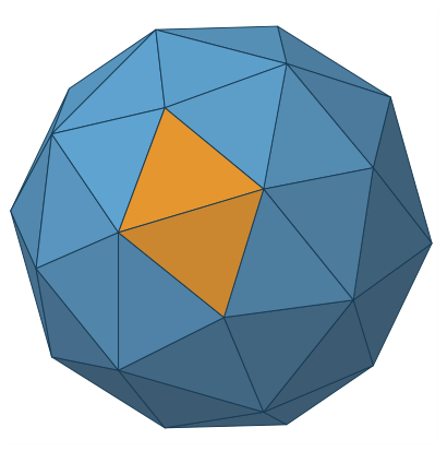
The first part of the architecture defines the geometric domain needed for base mesh face ownership, chart orientation, and spatial measurements. The Pentakis dodecahedron has 32 vertices, 90 edges, and 60 triangular faces. Each face defines one triangular chart, meaning one planar coordinate domain associated with that face. At each refinement, midpoint subdivision replaces one triangle with four smaller triangles. Level r therefore has segments along each base mesh edge and planar subtriangles per face before radial normalization to the sphere. Five triangular faces meet at some Pentakis vertices and six meet at others. Testing both arrangements verifies boundary transitions among different numbers of adjacent base mesh faces. Figure 3 shows the primary base mesh; the two index representations are introduced separately in Sections 3.3.1 and 3.3.2.
Geographic point assignment uses a face wise gnomonic construction: a longitude and latitude position is mapped to the spherical domain, centrally projected onto a candidate base mesh face plane, tested by barycentric containment, and discretized into the refined triangular chart. Deterministic ownership resolves positions on shared base mesh edges. The central projection has an important line preserving property: a great circle plane through the sphere center intersects a base mesh face plane in a straight line. Consequently, straight refined edges in the planar chart map back under radial normalization to great circle geodesic arcs, and the boundaries of the resulting spherical triangular cells are geodesic segments. Cell centroids are likewise reconstructed on the face plane and radially normalized to the sphere. The gnomonic construction is neither distance preserving, equal area, nor conformal, but its distortion belongs to the underlying mesh based DGGS rather than to the halo architecture. More importantly for the present method, projection is an indexing stage operation and is absent from the repeated preindexed adjacency expansion shown in Figure 5.
Figure 3.
The Pentakis dodecahedron used as the primary base mesh. Its 60 triangular faces define the planar charts from which refined spherical cells are constructed; two adjacent charts are highlighted in gold. The mesh has 32 vertices and 90 edges, corresponding to 180 directed base mesh edge transitions. Opaque face shading reveals the polyhedron’s three dimensional form.
3.2.2. Relating Topological Rings to Spatial Reach
A halo ring at topological distance k does not lie at a fixed spatial distance from the seed cells. Even on a uniform planar triangular grid, a path of k adjacency steps can turn in any direction, so topological distance k gives only an upper bound on spatial displacement, not a fixed multiple of a step length. On a DGGS the relationship is looser still, because projection distortion changes cell dimensions and shapes with resolution and with location across the base mesh faces. Exact distances between cells could be evaluated on the WGS84 ellipsoid with geodesic routines that account for the flattening of the Earth [35]. This subsection instead works on the spherical DGGS: cell centroids are radially reconstructed onto a sphere, and distances are evaluated as great circle arcs with one trigonometric operation per pair. The spatial extent of a completed ring is therefore characterized by the interval between the nearest and farthest such spherical centroid distances to the seed cells, as illustrated in Figure 4. These bounds are relative to the spherical model. Converting them to certified WGS84 intervals would require bounds that account for the adopted sphere, latitude, and direction; with the mean spherical radius used here and WGS84 flattening (), the local discrepancy near the poles is approximately relative to ellipsoidal distance. We retain the spherical bounds as a description of reach; whether K hops suffice to cover every location within a requested distance d requires both a coverage argument and explicit numerical limits, developed in Section 3.5.1.
The distances described above are between reconstructed cell centroids, not minimum distances between complete cell footprints. The quoted percentage describes the local polar limit for the adopted radius m; it is not a global error bound. At a pole, the WGS84 curvature radius is , giving a relative local difference of , with a and defined in Section 3.5.2. For a finite route the discrepancy depends on its locations and directions. It is not used in any coverage certificate. Section 3.5.2 retains the same cell adjacency but evaluates distances directly on WGS84 and bounds the corresponding mapped cell footprints. Its separate ellipsoidal tests do not rely on converting spherical centroid distances by a fixed percentage.
Figure 4 illustrates the distinction for one pair of cells and one adjacency route. Repeating the spherical distance calculation over every cell in a completed ring gives the nearest and farthest distances from the seed set. These ring measurements describe outward reach; the coverage test in Section 3.5.1 must also rule out required cells that have not yet been reached.
Here is the canonical seed set: the level r DGGS cells representing the input feature after duplicate public hierarchical indices have been removed. A symbol denotes one seed cell, whereas denotes one cell in the kth halo ring. Let be the unit vectors of their radially reconstructed spherical centroids, and let R be the adopted spherical Earth radius. Their cell to cell spatial distance is the minor arc great circle geodesic length
This form avoids subtracting nearly equal cosine values at centimeter separations. It is mathematically equivalent to the usual great circle formula, but a numerically stable formula alone is not a certified error bound. Using Equation (2), the distance from a ring centroid to its nearest seed centroid is
Here P is the same seed set defined in Section 3.1. This distance concerns the discrete seed centroids. It is not generally the distance to the original continuous source curve or to an entire seed cell.
For every nonempty topological ring , the nearest and farthest ring centroids give the exact query specific spatial interval
By Equation (4), every centroid in therefore lies between and meters from its nearest seed centroid. For a nonempty cumulative halo, its maximum centroid reach is . If the returned halo is empty, including when , spatial reach is reported as not applicable rather than taking a maximum over an empty set. These reductions annotate a completed ring and do not alter halo membership.
A bound on outward reach is useful even when the exact ring intervals are not evaluated. Define
as the longest spatial step permitted by one legal adjacency move anywhere in the level r grid, measured between the spherical centroids of adjacent cells. Every has an adjacency path of length k from at least one seed. The spherical triangle inequality therefore gives
Together, Equations (5) and (6) bound where an already reached ring can lie. A sampled maximum is not a certified value of . The zero is intentional: multiplying the minimum adjacent centroid step by k does not give a positive lower bound because the spatial route can turn. For distances between whole cells, let bound the distance from the reconstructed centroid to every point of any level r cell. Section 3.5.1 coverage derives such a bound from the base mesh. If distance between sets means their minimum point to point distance, then the distance from any ring cell footprint to the union of seed cell footprints lies in
The scale difference across levels is substantial. Near Calgary, the sampled adjacent centroid step at level 20 is approximately m. Four times that length is about 10 m. At level 28 the corresponding total is approximately cm. These are accumulated step scales, not minimum outward displacements: successive moves need not follow one geodesic. Neither these products nor guarantees coverage of a requested distance d. The inequality in Equation (6) gives an upper bound on reached distances, whereas completeness requires ruling out unreached cells within d.
The centroid distances in this subsection are evaluated after radial reconstruction on the sphere, not in a projected face plane. The gnomonic projection maps great circles to straight lines but is not distance preserving and has no single constant scale away from its center [36]; it therefore cannot by itself convert K into meters. Spherical offsetting similarly treats distance intrinsically on the sphere rather than as an uncorrected planar displacement [20]. All seed cells in one query must share a level. Mixed resolution neighborhood semantics and volumetric cells are outside the current scope.
3.3. Efficient Exact Halo Construction
The spherical interpretation shows why a ring count alone is not a distance guarantee. We first establish the reusable operation needed by both fixed hop and spatial distance queries: constructing complete rings from indexed seed cells. A cell representation must support persistent storage and hierarchy operations at the query interface, while allowing repeated adjacency and duplicate discovery with little work. This subsection introduces the two index representations and the local rules that connect them to the mesh.
Figure 5 shows the indexed halo component, not the complete spatial buffer procedure. Public hierarchical indices are converted once into compact integer triangular indices. Integer arithmetic constructs adjacent cells within a base mesh face, and an ACM record resolves a face boundary crossing. The CPU and GPU methods in Section 3.4 apply these rules to complete rings. Output indices are converted back after the requested expansion. The source cover and distance tests in Section 3.5 surround these calls and have their own cost.
This separation follows how often information is needed. Geographic geometry is used when creating the source cover and evaluating distances. Hierarchical decoding and encoding occur at the boundaries of a halo call. The repeated adjacency loop uses only integer coordinates, base mesh transitions, and the discovered set. Consequently, accelerating that loop does not remove the separate geometric work needed by a buffer query.
Figure 5.
Architecture overview. Public hierarchical indices are decoded once into compact integer triangular indices. The repeated traversal reconstructs adjacent cell indices, consults an Atlas of Connectivity Maps (ACM) record only at a base mesh edge, and constructs exact rings through the discovered set. Returned cells are encoded once after all requested rings are complete.
3.3.1. Public Hierarchical Index
The halo component receives cell indices rather than geographic coordinates. Its first requirement is a representation that identifies the input and output cells at the query interface. This representation must be persistent and reveal the base mesh face and resolution while supporting hierarchy operations before or after a halo query. The public hierarchical index is the unsigned 64 bit value accepted and returned by the query interface. Bit 63 is reserved and zero. Bits 62 through 57 store the base mesh face code. Bits 56 through 0 contain two bit child digits, followed by one level sentinel and trailing zeros. The prefix, sentinel, and padding convention, including recovery of the level from the least significant set bit, follows the mechanism documented for Google’s S2CellId [23]. Our adaptation assigns six bits to a triangular base mesh face code and supports 28 refinement digits. The base level sentinel is bit 56, and every refinement moves it two bits toward the least significant end. The 57 payload bits therefore hold 28 child digits and one sentinel.
The sentinel makes the level recoverable from the least significant set bit, and descendants of a cell share its prefix. Given a canonical level r public hierarchical index and a target level , an ancestor is computed by clearing the suffix below the target position and writing the target sentinel. The number of bit operations does not depend on . The same prefix defines a descendant interval at a target level. We retain this representation at the query boundary because databases, files, ancestor queries, and workflows with several resolutions require the level and hierarchy to be recoverable from the index itself. Repeating this hierarchy processing for every same level cell adjacency would add instructions and memory traffic to the dominant query operation.
3.3.2. Compact Integer Triangular Index
The public hierarchical index preserves the refinement sequence, but the repeated adjacency operation needs different information: during a fixed level halo query, every frontier cell must generate three neighbors and participate in hashing with little repeated work. Carrying the complete refinement prefix through that repeated loop would preserve information that is not used until the result leaves the query. We therefore define the compact integer triangular index. It is a transient 63 bit index used only inside the fixed level expansion; are its coordinate fields, and i and j are the two integer coordinates within the chart of one base mesh face. Its layout is
where for the Pentakis case, i and j are integer chart coordinates, is triangle orientation, and . For upward cells , ; for downward cells , . Figure 6 grounds these symbols in the subdivided chart of one base mesh face. Each 28 bit field stores integers from zero through , so the layout supports subdivisions along an edge and sets the maximum supported resolution to . The endpoint N is a geometric vertex coordinate, not a cell anchor stored in these fields. On a spherical Earth of radius km, the Pentakis cells have a global average area of approximately cm2. The square root of this average area is about cm, but it is not a triangle edge length or a certified cell diameter; individual areas and dimensions vary with projection distortion.
The relation to the continuous face coordinates is explicit. Let be the barycentric coordinates of the projected point, with , and set , , and . For a point strictly inside one refined cell, its discrete index is obtained by
Here . Equation 9 is an interior rule, not a complete rule for boundary ties. At a point on a refined edge or vertex, assignment must instead select a valid incident cell whose closed footprint contains the point. One complete mathematical convention selects the smallest unsigned public hierarchical index among all such incident cells, including cells on neighboring base mesh faces. For example, and touch , , and in the current face; the floor result is invalid. At chart vertices A, B, and C, the valid incident cells in that face are , , and , respectively. This exact ownership convention is a mathematical specification. The measured floating point mapper uses face selection, endpoint clamping, and cell validation; the current evidence does not certify all exact boundary decisions against that convention. Conservative source covering is different: it retains every touching cell, as required in Section 3.5.1.
The ratios and therefore describe the grid vertex at integer coordinates , whose barycentric coordinate is ; they are not, by themselves, the original continuous point coordinates. For completeness, the barycentric centroid of the indexed cell is
The two orientation cases in Equation (10) reconstruct the planar cell centroid before radial normalization. After this discretization, the same level adjacency phase operates strictly on ; the continuous barycentric values are no longer required.
Child numbering before table acceleration.
The conversion tables accelerate a fixed refinement rule, so that rule must first define what each public child digit means. Let a parent have integer anchor and orientation o, and let denote its child at the next level. A base mesh face begins at . Digit 3 selects the central child and changes orientation; digits 0, 1, and 2 select the three corner children according to Figure 7 and Table 1. Iterating these rules gives the same compact integer triangular index as geometric midpoint subdivision.
Each public hierarchical index is decoded once before the first frontier. A read only table with 512 entries processes four refinement digits per lookup. Its nine bit lookup key contains the current orientation bit and the next four two bit child digits. Each entry returns the increments of i and j and the orientation after those four refinements. A level 28 public hierarchical index therefore requires seven lookups instead of 28 separate child steps. A second table with 512 entries performs the reverse conversion four levels at a time. It uses the current orientation and the lowest four bits of both i and j to recover four child digits and the parent orientation. The storage of both tables is fixed and does not depend on the resolution. Output cells are converted to public hierarchical indices only after all halo rings are complete. This placement avoids decoding a public hierarchical index for every generated candidate, while preserving the persistent representation needed by storage and hierarchy operations.
3.3.3. Comparison with BIM and Design Rationale
The preceding subsection introduced the compact integer triangular index for the repeated adjacency operation. This subsection documents its storage and operation requirements in relation to the more general Barycentric Indexing Method (BIM), rather than predicting a GPU speedup from coordinate counts. The two indexes share a barycentric foundation but serve different purposes and are not competing public DGGS standards. The published BIM index is . It combines a base cell index and an explicit resolution w with the symmetric three axis integer coordinate . BIM supports geometric, hierarchical, and neighborhood operations across watertight triangular meshes, and its Atlas of Connectivity Maps extension preserves these operations across base mesh boundaries [8]. Our compact integer triangular index is a temporary representation for one halo query at a shared resolution. The public hierarchical index remains the externally visible cell representation.
BIM retains three symmetric axes even though normalized barycentric coordinates have two independent degrees of freedom. As described in the BIM paper, its integer coordinate image is sparse, so some integer triplets do not represent cells. Point indexing near exceptional vertex configurations can therefore require a validity check and a small correction to select a represented cell [8]. Adjacency within one base triangle remains constant time because one of a, b, or c is incremented or decremented according to orientation. When an adjacency crosses a base mesh edge, the crossing axis and destination orientation determine one of three coordinate permutations: , , or is exchanged. This symmetry is valuable in a general mesh index. A direct tuple of three 28 bit coordinates occupies 84 coordinate bits, but that is not a lower bound on a packed BIM index. At a shared level, the permitted coordinate sums and a triangle type bit allow one coordinate to be reconstructed from the other two. The BIM paper explicitly discusses two coordinates plus one distinguishing bit. A specialized packed BIM key could therefore also fit two 28 bit fields, a 6 bit face field, and one type bit in 63 bits. Our choice is that the stored fields directly serve the implemented adjacency and hash operations, not that BIM inherently requires a multiple word key.
The compact integer triangular index omits state that does not change during this narrower workload. The level r is common to every seed, frontier, discovered, and output cell, so it is stored once for the query. After discretization, provide the two independent chart directions, and o distinguishes upward and downward elementary triangles. Every tuple that satisfies the relevant triangular domain condition represents one cell. Adjacency inside a base mesh face therefore uses the fixed offsets in Equations (11) and (12), without introducing a third coordinate into the interior operation. Valid cell traversal should not be confused with point assignment: this does not imply that BIM corrects an invalid triplet after every neighbor step. A base mesh edge crossing still requires a boundary decision, but one atlas record maps a scalar edge position using either or . Together with the base mesh face code f, these fields form the 63 bit layout in Equation (8). Figure 8 the coordinate conventions and boundary operations used during a query.

Table 2.
Coordinate conventions and execution roles. The comparison follows the published BIM operations; it claims neither an inherent packed storage advantage nor measured superiority over an optimized BIM implementation.
Table 2.
Coordinate conventions and execution roles. The comparison follows the published BIM operations; it claims neither an inherent packed storage advantage nor measured superiority over an optimized BIM implementation.
| Design concern | BIM index | Compact integer triangular index | Halo query consequence |
|---|---|---|---|
| Coordinate image | Symmetric image is sparse; exceptional point assignment may require checks | Every tuple satisfying the explicit domain conditions represents a cell | Both methods distinguish point assignment from traversal of valid cells |
| State at level 28 | A packed form can retain two coordinates and a triangle type, with face and query level | uses 63 bits; r is query wide | Both can support a single word key; packing alone does not prove a speed advantage |
| Interior adjacency | Increment or decrement one of three axes according to orientation | Three fixed offsets and an orientation change | Two coordinate fields and no hierarchy decoding in the repeated loop |
| Base mesh boundary crossing | Detect the boundary axis and select one of three axis exchanges | Apply one of the atlas records to scalar edge position t | Different coordinate rules; both need boundary handling and implementation dependent instructions |
| Intended role | General geometry, hierarchy, and movement operations | Adjacency expansion and set membership at one shared level | Generality remains at the public boundary; compact state serves the repeated query operation |
Table 2 summarizes the design tradeoff. The complete compact integer triangular index fits one 64 bit discovery word, but a storage collision can still require several probes. BIM could use precomputed transformations or a different packing scheme; instruction counts and thread divergence depend on the implementation and compiler. We therefore make no measured GPU performance claim against an optimized BIM implementation. The conversion ablation in Section 4.1.2 instead compares keeping our compact integer triangular index throughout a query with repeatedly converting our public hierarchical index.
3.3.4. Implicit Local Adjacency
With the index roles established, we can derive the operation performed for every frontier cell. Inside one base mesh face, crossing an edge changes an upward triangle into a downward triangle, or conversely. The adjacent triangle either uses the same integer position or differs by one in one coordinate. These three possibilities give the fixed adjacency equations:
If a candidate satisfies the triangular domain conditions, it remains on face f and is encoded directly. Therefore, an adjacency inside one base mesh face performs no table lookup and loads no stored neighbor record. This reconstruction is the central scalability choice: storing three neighbor indices for every refined cell would require storage proportional to the complete level, whereas the arithmetic cost remains constant at every resolution.
3.3.5. Base Mesh Edge Atlas
The interior rules are sufficient only while the adjacent cell remains on the same face. At a base mesh edge, the query must identify the neighboring face and express the adjacent cell in that face’s coordinates. The ACM stores this relation once for each directed base mesh edge. For source face f and one of its three edges e, the record
stores the destination base mesh face g, destination base mesh edge , and an edge direction reversal bit . If is the discrete position of the source boundary cell along edge e, then
The destination edge and mapped position select one of three fixed boundary templates, which reconstructs the destination compact integer triangular index . Thus, t and are local edge positions, not cell indices. In concrete terms, the ACM record answers the otherwise ambiguous boundary question: “which base mesh face owns the neighbor across this edge, which of its three edges is shared, and in which direction are the discrete edge positions ordered?” For a triangular base mesh with F faces, the atlas has exactly directed records and is independent of refinement level. Pentakis has records and occupies 720 bytes in the packed representation; an icosahedron has 60 records and an octahedron has 24. The table resides in device constant memory because it is small, does not change during a query, and can be shared by threads crossing the same base mesh edge. Figure 9 contrasts the arithmetic only interior case with the exceptional boundary case that consults this record.
Table 3 completes this reconstruction. Edge 0 is the side opposite chart vertex A, edge 1 is opposite B, and edge 2 is opposite C, using the axes in Figure 6. Every cell sharing an edge with a base mesh boundary has upward orientation. For example, , destination edge , and mapped position reconstruct the destination cell . Packing that tuple, not the scalar , gives the destination compact integer triangular index.
The transition records must agree with the mesh geometry, not merely with another implementation using the same records. We generate the table from a directed edge representation, which records each face’s side of every base mesh edge. Independent references then check both the base transitions and complete refined edge pairs without consulting the runtime ACM. Section 3.6.6 gives the construction and test coverage. This separates the mechanism used to cross a face boundary from the evidence that the crossing is correct.
3.4. From Local Adjacency to Complete Rings
Section 3.3 established how one cell is represented and how its three edge adjacent cell indices are reconstructed. A complete halo query must coordinate these constant cost operations over every cell in the current ring while preserving the recurrence in Equation (1). At the start of iteration k, the frontier is the completed ring and the discovered set satisfies
A candidate belongs to exactly when its compact integer triangular index is absent from V. This section first establishes the serial and multithreaded CPU realizations of that invariant. It then defines the GPU resident query state, the exact hash address and collision procedure, concurrent first discovery, synchronization between rings, capacity checks, and resource bounds. These steps answer the collective set construction question that remains after adjacency has been reconstructed for one cell.
3.4.1. Serial and Multithreaded CPU Traversal
The CPU implementations establish the ring recurrence and provide performance baselines with different storage and synchronization costs. All accept and return public hierarchical indices, use the same compact integer triangular indices and adjacency rules, and construct the same ring sets. Agreement checks execution consistency; independent geometry tests are still needed to validate their shared atlas.
The serial container implementation preloads the compact seed indices into a node based hash set and stores in the frontier. For every frontier cell it constructs three adjacent indices and appends an index to the next ring only if insertion reports that the index was absent. This implements Equation (15). The serial flat table baseline replaces that container with an array of open addressed slots. It uses the mixing and linear probing rule defined in Section 3.4.3 and retains table capacity between calls. This separates node allocation and pointer access from the cost of the recurrence.
Parallel processing also needs to coordinate insertions. The partitioned implementation uses the OpenMP shared memory programming interface to generate candidates, groups them by a hash selected shard through count and scatter, and gives each shard to one worker. The shard count is the next power of two above for T threads, giving 256 shards at twenty threads. Each worker inserts into its shard without locks. New indices are concatenated after each ring. This design measures the cost of grouping and node based sets; it is not the primary multithreaded baseline.
The multithreaded flat table is the primary parallel CPU baseline. The primary matrix runs it with twenty threads, so the results refer to it as the twenty thread flat table; the thread sweep in Section 4.1.1 varies that count. It uses atomic compare and exchange to claim slots in a shared open addressed table. Each worker collects new cells in a private buffer; separately aligned headers reduce sharing of frequently updated counters. Dynamic scheduling distributes frontier work across the workstation’s performance and efficiency cores. Expansion and concatenation use separate OpenMP regions, with implicit synchronization at region boundaries; output encoding is also parallel. The CPU and GPU therefore share the membership and complete ring principles, but not an identical instruction sequence or barrier count. CPU output is materialized in a newly allocated returned container.
The flat table designs remove the node based set as the sole CPU reference. Section 4.1.1 compares both flat table baselines with the GPU and reports a thread count sweep. The serial container and partitioned implementations remain diagnostics of the baseline choice. The order of indices within a ring is unspecified; ring membership and ring offsets determine correctness.
3.4.2. GPU Resident State and Query Stages
A halo query is iterative: ring must be completed before it can serve as the frontier for constructing . If each completed ring is returned to the CPU, every iteration requires GPU synchronization, transfer of intermediate state, a CPU decision about the next frontier, and another GPU launch. Because generating the three adjacent cells requires only a small amount of arithmetic, this repeated coordination can cost more than the adjacency operation itself. The purpose of the GPU resident design is therefore to retain the complete iterative state in GPU memory and execute all requested rings without transferring intermediate frontiers to the CPU. Figure 5 shows this placement: conversion occurs at the query boundaries, while adjacency expansion and discovery remain on the GPU.
Each GPU resident structure supports a specific part of the recurrence. The unique compact seed array initializes . The discovered set V records the seed cells and every cell admitted to a halo ring, allowing later candidates to be rejected without consulting the CPU. The cumulative compact output stores the discovered halo cells and provides the frontier slices used by subsequent iterations. The ring offsets identify where each ring begins and ends, while device counters and an error status coordinate output allocation and report bounded failures. These structures remain in GPU memory throughout the expansion. Public hierarchical indices are used only in the input and output arrays and do not replace the compact integer triangular indices used by repeated adjacency and discovery operations.
The resulting query follows the four stages illustrated in Figure 5. First, the public hierarchical input indices are copied once to the GPU, validated, decoded, and deduplicated to form in compact form. Second, all requested ring iterations construct adjacent cell indices, test discovery, and append new cells while the discovered set, frontier slices, and ring offsets remain on the GPU. The final control state and completed ring offsets are then read by the CPU. Third, after the final ring is complete, the compact output indices are encoded into public hierarchical indices. Fourth, the encoded cell indices are copied once to the CPU. This separation also defines the reported timing components. Seed decoding and expansion share one kernel, but their recorded traversal interval also includes final control and ring offset readback, synchronization, and the intervening host scheduling interval before the end event is recorded. Output encoding and the bulk cell array transfer are measured separately; the traversal interval is not a pure kernel measurement. Geographic point projection is not part of this preindexed query.
3.4.3. Hash Function and Open Addressed Discovered Set
During a parallel frontier expansion, potentially thousands of GPU threads simultaneously construct adjacent cell indices. Different frontier cells can share the same adjacent cell, so several threads may generate an identical candidate. To preserve exact set semantics, the architecture must admit that cell to the new halo ring only once and reject it if it already belongs to the seed set or a completed ring. We support this decision using a GPU resident, open addressed hash table that stores the discovered set V. In an open addressed table, cell indices are stored directly in an array of slots. A lookup checks a sequence of slots until it finds the index or an empty location. Each slot check is called a probe. The following paragraphs explain how the sequence is chosen and how concurrent insertions are resolved.
Candidate construction produces one 63 bit compact integer triangular index x for each adjacent cell. The packed face and coordinate fields are spatially correlated, so directly using selected bits of x could place many nearby cells in the same part of the table. The mixing function spreads these patterns before table addressing. It applies a fixed sequence of 64 bit addition, bitwise exclusive OR with shifted values, and multiplication by odd constants, following a standard SplitMix style integer mixing procedure [37]. These operations determine only the table location associated with x; they do not modify the compact integer triangular index itself.
Let the table capacity be . Probe number ℓ addresses
where & denotes bitwise AND. Because M is a power of two, masking with maps the mixed value to a valid table slot. The first probe uses . If that slot contains a different index, linear probing advances through until the operation finds an empty slot, finds x, or exhausts the table [38].
Every valid compact integer triangular index has bit 63 equal to zero. The all ones word
can therefore represent an empty slot without conflicting with a valid cell index. The logical claim attempts to replace E with x atomically. The implementation first reads the slot and avoids the atomic operation when it is already occupied; Section 3.4.6 explains this optimization. When a claim is attempted, its returned value produces three outcomes:
- 1.
- If the returned value is E, this thread inserted x and discovered a new halo cell.
- 2.
- If the returned value is x, the index is already present, so the thread stops without appending it again.
- 3.
- If the returned value is another index , a storage collision occurred, so the thread advances to the next probe position.
The table is cleared before each query and preloaded with the unique seed indices. Every newly discovered halo index remains in the table for the rest of the query. No deletion occurs, so the table needs no additional marker for a deleted entry. Consequently, an index already present in the table may represent a seed cell, a cell discovered in an earlier ring, or the same candidate inserted by another thread during the current ring. All three cases require the same action: reject the candidate because it must not be appended again.
The target load
is at most . Under the standard assumption that the mixing function distributes indices across the table, this bounded load keeps the expected number of probes constant. Fewer probes reduce global memory accesses and contention among threads attempting to claim nearby slots. The explicit limit of M probes guarantees termination; exhausting all slots reports insufficient hash capacity instead of returning an incomplete halo. A different resident index y is therefore a hash storage collision, not a statement about spatial adjacency or halo membership.
Figure 10 connects this storage procedure to the spatial operation. It follows one adjacent cell from triangular candidate construction, through the 64 bit mixing function, to the atomic decision that appends the cell, rejects it as already present, or continues probing after a storage collision.
Figure 10.
From triangular adjacency to atomic candidate discovery. A one into four refinement exposes the three edge adjacent candidates of a frontier cell . One candidate is represented by the compact integer triangular index x and passed through the 64 bit mixing function to select an initial probe slot. The atomic compare and swap returns Empty when x is first discovered, x when it is already present, or a different resident index y when a storage collision requires probing the next slot. Only the first outcome appends x to the new halo ring .
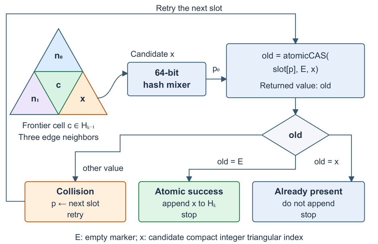
One table slot stores the complete compact integer triangular index, and one successful native 64 bit atomic compare and swap claims an empty slot for that index. A discovery may still require several probes and atomic attempts before it terminates. Output reservation is a separate atomic operation, described next. This distinction is important when interpreting the representation choice in Section 3.3.3.
3.4.4. Atomic First Discovery and Next Ring Construction
The hash procedure defines storage outcomes; the halo recurrence requires a set membership decision. This subsection establishes the correspondence between them. A lookup has two terminal membership results: the candidate is newly inserted or its compact integer triangular index is already present. The already present result has three possible query histories: the index belongs to the seed set, it was inserted in an earlier ring, or another worker inserted it during the current ring. Together with a successful insertion of a new cell, these are the four query meanings. The GPU resident hash table intentionally stores only membership, not the history that caused an existing index to be rejected.
The compare and swap that changes an empty slot from E to x is the instant at which the cell becomes discovered. This is the operation’s linearization point: although several workers may attempt discovery concurrently, only one can make that successful change. That worker alone may append x to the output for . Workers that subsequently find x already present do not append it again.
Appending each accepted cell with a separate global counter update would create another shared point of contention. The implementation therefore combines appends within a warp, a group of 32 GPU threads, following the warp aggregated atomic technique documented by NVIDIA [39]. A ballot operation produces a bit mask identifying which threads successfully discovered cells. One thread reserves a consecutive output range for that group, and each successful thread uses its position among the set bits to select a unique location in the range. This reduces counter updates while preserving one append per discovered cell. Together, atomic discovery and grouped append construct the next ring without a separate candidate array, global sorting, and subsequent set subtraction.
3.4.5. Cooperative Multiple Ring Execution
Atomic insertion resolves individual discoveries, but a later ring must not begin until every cell in the current ring has been processed. This dependency requires synchronization across the workers, not a new distance or membership rule. GPU threads are organized into blocks, and the collection of blocks launched for a query is called a grid. The cooperative implementation limits the grid so that its blocks can remain resident together. Threads process successive frontier cells in strides, allowing that bounded grid to handle larger rings. A grid wide barrier waits for discovery to finish, one designated worker records the ring’s output boundary, and a second barrier makes that boundary visible before the next iteration. The new output slice then becomes the next frontier without returning its size to the CPU.
Algorithm 2 summarizes the device resident control flow. The notation Insert includes the mixing, probing, and atomic claim defined in Section 3.4.3; WarpAppend denotes the aggregated output reservation described above.
| Algorithm 2 GPU resident halo traversal |
|
The reported RTX 4070 measurements use this cooperative schedule. The implementation also synchronizes after one worker prepares the control state at the start of each iteration. Including the two barriers shown after expansion, it executes three grid wide synchronization points per hop and initialization synchronization before the loop. The primary fused decode and expansion kernel has two initialization barriers; the separately timed expansion kernel in the buffer study has one. Algorithm 2 expresses the ring dependency; this additional barrier makes its loop control safe across the grid. An automatic scheduling mode selects a host driven kernel per ring fallback when cooperative launch is unavailable; the fallback preserves the same ring sets but transfers control to the host between iterations. If the caller explicitly requests the cooperative schedule on unsupported hardware, the query reports that condition rather than silently changing the requested mode. When , no ring expansion is performed and the returned halo is empty. In every schedule, the order of indices within one ring is unspecified.
3.4.6. Probe Reduction and Output Delivery
Keeping rings on the GPU removes intermediate host transfers, but not redundant discovery work or the cost of delivering a large result. Four mechanisms reduce those costs without changing the set recurrence. Their individual and combined effects are evaluated in Section 4.1.2.
Arrival edge skipping.
Every new cell was reached across a shared edge from a cell already discovered. The successful worker stores that reverse edge number in one byte beside the new output index. For an interior move, the orientation specific equations determine the reverse edge; for a base mesh crossing, the atlas gives the destination edge (). When the new cell is later expanded, this one neighbor is known to be discovered and need not be submitted for hash lookup again. The implementation still constructs all three geometric neighbors before skipping that lookup. Seeds have no recorded parent and submit three neighbors for lookup; later frontier cells submit two. The successful claim selects one parent, and ring synchronization completes its record before the next expansion.
Read before compare and swap.
An unsuccessful discovery often needs only to establish that an index is already present. The implementation uses a 64 bit global load that bypasses the first level cache to inspect a slot, and attempts atomic compare and swap only after reading the empty marker. An occupied slot never changes during a query. At the algorithmic level, an older empty value leads to an atomic attempt that resolves the current slot, while an occupied value permits direct comparison. This monotone state argument motivates the optimization. The current load is a cache controlled load of the Compute Unified Device Architecture (CUDA), not a C++ atomic load; output agreement tests are implementation evidence rather than a formal proof of device memory ordering.
Page locked output staging.
The query object retains a page locked (pinned) host buffer across calls. These pages are not paged out by the operating system during the transfer. Encoded output is copied directly into this buffer without allocating and initializing a new pageable result vector inside the readiness timer. The instrumented interval ends when the public indices are available in the pinned host buffer and the ring offsets have reached their separate host result vector. The query interface then copies the indices into its returned cell vector before returning to the caller. We therefore distinguish pinned host readiness from returned container completion; the former is not the complete call latency of the query interface.
Fused control initialization.
Counters and status words are grouped into one control allocation and cleared together. Free device memory is queried when buffers need to grow rather than on every call with sufficient retained capacity. Growth and capacity failure remain checked. This fourth mechanism bundles two reductions in fixed per call work; its ablation does not separate their individual effects.
These choices add one arrival byte per output capacity slot and retain host staging memory between calls. They are implementation techniques rather than new DGGS indexing principles. The timing boundaries in Table 6 distinguish their computation and delivery costs.
In the remainder of the paper, the GPU implementation denotes the cooperative implementation with all four mechanisms enabled. The four mechanism removal variant disables these options in the current source for a controlled comparison. We distinguish it from the earlier GPU release, which predates these mechanisms and supplies the historical schedule and global validation evidence. The E3 configuration and the separate WGS84 implementation also retain their own recorded build and timing scope (). Similar option settings do not establish identical source versions.
3.4.7. Capacity Planning and Explicit Failure
Keeping several rings inside one GPU launch also constrains memory allocation. All workers must continue using the same hash table and output addresses while the grid synchronizes, so these arrays are allocated before the launch rather than moved during it. The query therefore needs an explicit capacity estimate and a defined response when that estimate is insufficient. For the Pentakis implementation, the automatic output budget is
where is the input count before deduplication. This expression follows the ring growth of the regular triangular cell adjacency and is used as the allocation budget for the Pentakis implementation. It is not asserted as a universal bound for every triangular base mesh. A different base mesh may supply a justified budget or use the topology independent degree three tree bound . The caller may also supply an explicit maximum output count. In every case, the capacity checks below protect result completeness if the supplied budget is insufficient.
For an output capacity B, the table capacity is
which keeps occupancy at or below 50% when the result stays within B. Before buffers grow, a memory preflight rejects a request whose required allocation exceeds 85% of currently available device memory. During execution, separate status values report invalid or noncanonical input indices, mixed input levels, exhausted hash capacity, and exhausted output capacity. No partial halo is returned after any of these conditions. The caller may resubmit with a larger explicit bound or route the query to the CPU. Explicit failure and retry are used instead of during launch reallocation because moving the table or output array would invalidate addresses shared across the cooperative grid.
The recorded workspace metric can be reconstructed from these capacities. With M hash slots, two output arrays and an arrival byte array of capacity B, two input arrays of capacity , and ring offsets, its reported value is
This expression reproduces the 81 workspace values recorded in the primary matrix. The term counts two 64 bit output arrays and one arrival byte per slot. It remains a reporting metric: the source allocates a 128 byte control block but counts 96 bytes, underreporting explicit device payload by 32 bytes at fresh capacities. Runtime state, static device data, allocator overhead, and the pinned host buffer are excluded. Retained allocations can also exceed the capacities requested by a subsequent smaller query. We preserve the recorded measurements and state their accounting boundary.
The automatic budget grows quadratically with depth even when overlap makes the realized halo much smaller. Its admissible input count therefore depends on the currently free memory and power of two table sizes, not a fixed fraction of nominal GPU capacity. The recorded boundary buffer experiment instead supplies an explicit output capacity of 200,000 cells to each call. Input storage and discovered set capacity remain separate; this is not a 200,000 cell limit on their combined occupancy. Exceeding the output capacity still causes explicit failure.
3.4.8. Complexity and Storage
We can now distinguish the work performed by the query from the memory reserved to execute it. This distinction matters because a conservative capacity estimate can exceed the number of cells actually discovered. Let denote the returned halo. Every expanded cell has three edge adjacent cells. To compare schedules consistently, we count the logical adjacency work before redundant parent edges are skipped:
Under the bounded load and distribution assumption stated in Section 3.4.3, expected adjacency and discovery work is . The current implementation still constructs those W geometric neighbors, but arrival edge skipping removes some before discovery; W is therefore not the number of lookup candidates, slot probes, or atomic instructions. Hash probing is not claimed to be constant in the deterministic worst case: one candidate may inspect at most M slots before reporting capacity exhaustion. Input decoding processes supplied indices and costs , even when duplicates reduce the unique seed set substantially. Clearing the hash table costs , and output encoding and materialization cost at the supported maximum level. The cooperative traversal also performs three grid wide synchronization points per requested ring, plus initial launch synchronization. These initialization and synchronization costs help explain why adjacency throughput alone does not predict the latency of a small query.
The base mesh topology occupies exactly ACM records, or static storage. Occupied query state contains distinct cells, but allocated storage must also include unused capacity reserved before the cooperative launch. With M discovered set slots, input indices, an output capacity B, and ring offsets, the actual allocation is
When the reserved capacities are within a constant factor of the realized unique input and output sizes, this reduces to . The automatic budget can reserve more memory when seed neighborhoods overlap or the input contains many duplicates; output sensitive occupancy does not by itself imply an equally tight allocation. In either case, storage is determined by the query and its chosen capacity, not by materializing the cells or their refined adjacency records.
3.5. From Halo Rings to Spatial Buffers
The preceding method constructs exact rings from indexed seed cells, but it does not determine how many rings a distance request requires. A complete spatial buffer additionally requires a cover of the continuous source, a stopping condition that rules out undiscovered target cells, and a distance test applied to discovered cells. We now define these requirements independently of the execution method, first on the sphere and then in the numerical WGS84 boundary implementation.
3.5.1. Conservative Distance Coverage with Bounded Surplus
A request expressed in kilometers asks for complete spatial coverage, not a particular number of rings. In the Nose Hill Park example, every location in the 1 km buffer must be covered even where its boundary cuts through a cell. We now state the conditions needed to obtain that guarantee on the spherical DGGS, rather than only in the projected illustration. The basic idea is to continue exact ring expansion until an entire frontier is certified to lie beyond the requested distance, then retain all cells that could intersect the requested buffer. Uncertain boundary cells remain in the answer. Their maximum surplus distance is bounded by the cell extent, so precision can be chosen through the resolution without accepting omissions. This formulation follows the conservative inclusion principles of spherical offsetting and continuous coverage [20,21]; it adds a stopping certificate around our exact halo recurrence.
The region that must be covered.
Let be a nonempty closed source geometry on the adopted sphere, and let be the requested distance in meters. For the running example, is the complete park boundary curve and m. The definition also permits a filled polygon if its complete cell cover is supplied. Define
where is the closed spherical footprint of cell c and distance to means the shortest great circle distance to any point of that geometry. contains all and only the cells that intersect the buffer, including its boundary. We call this the exact cell intersection set. A conservative returned set must contain , but may include cells that do not intersect the buffer. We also require its complete footprints to remain inside for a stated surplus width . These are separate requirements: no missing cells and a bounded outer extent.
The seed set must include every cell whose closed footprint intersects . In particular, a point or curve on a cell edge or vertex contributes all touching cells; the unique ownership rule used for ordinary point indexing is not sufficient for this cover. The same formulation can accept other source geometries. A filled polygon includes its interior. A boundary curve, such as a park boundary or a shoreline, instead produces a buffer on both sides of the curve, and all components and islands must be included. A filled polygon must not silently replace a boundary curve.
A conservative cell distance test.
We need a test that cannot discard a cell merely because its centroid lies just beyond d. Let be its reconstructed spherical centroid and let be a certified upper bound for every distance from to a point of . Suppose a geometric routine supplies an interval containing , with width at most . The triangle inequality gives a lower bound for distance from the whole cell to the source:
The conservative acceptance test is . Equality and unresolved numerical cases are retained. A comparison of the centroid distance alone with d would miss cells that straddle the requested boundary. The interval routine must bound distance to the complete source geometry, not only its sampled points; outward rounding must also be used when forming the test and its radius bound.
Certifying how many rings are sufficient.
We keep the topological recurrence unchanged and write for all discovered cells, including the seeds. Starting from the complete source cover, expand rings until the first tested for which
The resulting depth is denoted by ; the minimum is evaluated only for a nonempty frontier. It is taken over the entire ring, across every source component and every base mesh face. A camera view, a few boundary cells, or a mean step length cannot replace this test. Intermediate rings are not pruned by the distance test, so their original minimum topological distances remain unchanged. If a valid upper estimate of K is available it can schedule work, but acceptance of the result still requires the certificate.
Proposition 1
(Sufficiency of the whole ring stopping test). Assume a finite, conforming triangular tessellation of the sphere with closed cell footprints and connected incident cell fans. Let be nonempty and closed, let P contain every cell touching , and let every be a valid lower bound on distance from the whole footprint to . If the complete rings satisfy Equation (24) at depth K, then every cell in belongs to .
Proof.
For a cell in , select a point where its footprint meets . A shortest spherical arc to a nearest point of exists and remains in . Cells intersected by this arc connect to a seed through edge adjacency. At an edge or vertex contact, include all touching closed cells; the connected incident fan supplies an edge adjacent route, and every included cell still intersects the buffer. If the target were outside , this route from a seed would cross , because minimum adjacency depth changes by at most one across an edge. That crossing cell has , contradicting the nonempty ring condition in Equation (24). If is empty, no further cell is reachable from the seeds; the same route again excludes an undiscovered target. □
Proposition 1 is a geometric statement under explicit assumptions, not a proof that floating point arithmetic produces the required bounds. The WGS84 extension must satisfy the corresponding assumptions in its own metric; its numerical checks are reported separately.
After certification, retain
The seed ring is included when selecting this distance result, although the topological halo H excludes it. Otherwise, a requested location inside a seed cell could be omitted. The complete procedure is stated in 3.
| Algorithm 3 Conservative distance cover using complete halo rings |
|
Bounding additional coverage.
The same cell radius that prevents omissions bounds the excess. For an accepted cell, and its true centroid distance is at most . Every point in that cell is therefore at most from . Assuming complete source covering and valid distance intervals, with , the mathematical result satisfies
This bounds the additional distance, not the percentage of extra cells or area. Those percentages depend on the length and shape of the source and on the land distribution around it. A bound on alone provides neither inclusion in Equation (26).
The cell radius can be bounded without enumerating the refined grid. For base mesh face f, let be its planar centroid, its plane distance from the sphere center, and the maximum Euclidean distance from to its three vertices. Midpoint subdivision scales every planar cell by . Along a segment in that plane, radial normalization changes angle by at most per unit planar distance. Any radius value satisfying
bounds the distance from each normalized planar centroid to every point of its spherical cell. The maximum involves only base mesh faces. Adjacent cells share a point, so the same argument gives and therefore , still only an outward reach bound. The accompanying exact rational check verifies for all 60 faces of the frozen Pentakis mesh, a serialized and checksummed copy of the base mesh. Using with m gives the rounded upward bounds in Table 4. This check certifies the mesh constant relative to its serialized coordinates; it does not certify an untested geographic distance routine or establish that every performance experiment used a byte identical mesh file.
The guarantee is relative to the supplied geometry, the chosen Earth model, and certified arithmetic. A spherical 10 km distance is not identical to a World Geodetic System 1984 ellipsoidal distance. An ellipsoidal contract requires compatible geodesic routines and corresponding bounds [35]. An incomplete source dataset or an unbounded numerical approximation cannot support a claim of complete real world coverage.
The preindexed traversal measurements evaluate the fixed K recurrence. The GPU returns complete topological rings and does not itself trim them against the spatial buffer. The separate extension below adds source covering, whole ring stopping tests, and cell filtering. Unknown requires a capacity limit and either resumable expansion or safe replay; a capacity error does not permit an incomplete answer. Cell filtering examines all visited cells, including seeds, rather than only the final ring. Even the exact cell intersection set generally extends beyond a continuous distance contour when its whole cells are displayed. Matching that contour exactly would require clipped cell geometry.
3.5.2. WGS84 Boundary Buffers and Numerical Implementation
The spherical formulation explains why whole ring tests can establish coverage. A request measured on WGS84 needs the same reasoning with an ellipsoidal metric and the actual curved cell footprints. We therefore retain the same ring recurrence and add an ellipsoidal source cover, stopping test, and cell distance filter. Its source is the union of the supplied shortest WGS84 geodesic segments. Polygon rings contribute their boundaries, not their filled interiors. All components are preserved. This matches the boundary request introduced in Figure 1, including any central region that is excluded because it lies farther than d from the curve. Interpreting the input segments as geodesics is explicit because generic GeoJSON edges are not defined that way.
The WGS84 model has equatorial radius m and flattening . Direct and inverse geodesic calculations use GeographicLib and the algorithms of Karney [35]. The spherical DGGS longitude and latitude become geodetic longitude and latitude on WGS84. This mapping preserves the cell indices and adjacency. It does not replace cell edges by shortest ellipsoidal segments: each footprint is the image of the complete radially projected planar triangle.
To bound these footprints, let and let and denote the meridional and prime vertical radii of curvature at geodetic latitude . Both are bounded above by m. The ellipsoidal line element is therefore at most times the corresponding unit sphere line element. For any planar triangular patch inside base mesh face f, let be its greatest vertex distance from its planar centroid. The same radial derivative argument as in Equation (27) gives
as a geometric radius bound in meters before numerical allowances. This applies to the actual curved footprint, including interior points. The verified base ratio gives rounded upward whole cell bounds of m at level 20 and m at level 28. The spherical values in Table 4 must not be substituted for these ellipsoidal values.
Distance to one source segment.
The cell test needs the distance from a point to the complete source curve, not only its vertices. Let be one segment parameterized by geodesic arc length. Let and be the WGS84 distances from a query point q to its endpoints. Before numerical allowances, the triangle inequality gives
The endpoint distances give an upper bound because those endpoints belong to the segment. The lower bound follows because distance to q can change by no more than the distance traveled along the segment. Evaluating its geodesic midpoint creates two shorter intervals with their own endpoint bounds. The routine repeatedly divides the interval with the smallest lower bound, retaining the best sampled upper bound, until their difference meets the requested tolerance.
For a synthetic arithmetic example, a segment of length 10 m with endpoint distances both 13 m gives m in Equation (29). If its midpoint distance is 12 m, the combined interval tightens to m. This explains interval refinement; it is not a measured DGGS query.
Searching a complete boundary efficiently.
Most segments of a detailed boundary cannot contain the nearest point. A segment of length s is enclosed by a metric ball centered at its geodesic midpoint with radius . Groups of segments are enclosed by larger balls: for a chosen group center, the radius is the maximum distance to a member segment midpoint plus that segment’s radius. The triangle inequality guarantees containment. Distance to the group center minus its radius supplies a lower bound. A group is skipped only when this bound exceeds an already established upper bound on the nearest source distance. The hierarchy reduces search work without replacing the source by samples.
Covering the complete source.
Source covering starts with every base mesh face. The point to source interval and patch radius give a lower bound on the distance from each closed triangular patch to the source. A patch is discarded only when that lower bound is strictly positive; remaining patches are refined to the query resolution. Equality is retained. A source touching a shared edge or vertex is therefore covered by every incident touching cell, rather than assigned to one owner. This statement assumes valid numerical bounds. It explains why the point ownership convention used for ordinary indexing is not used for source covering.
Stopping expansion and filtering cells.
The host loop requests complete halo queries at depths until the entire final ring has footprint distance lower bounds greater than d. Each request replays the recurrence from the same seed set. Iterations within a GPU halo call remain on the device, but distance tests between calls run on the CPU. The complete boundary workflow is therefore hybrid.
Final filtering examines every discovered cell, including the seeds. A lower bound greater than d excludes a footprint; an upper bound at or below d confirms intersection. For an uncertain cell, subdivision tightens the bounds over its curved footprint. This subdivision is internal to the geometric test: it does not change the cell’s public hierarchical index or the query’s output resolution. Cells still uncertain when a stopping threshold or evaluation budget is reached are retained and labeled. A finer query resolution instead changes the returned cell size and is a separate choice.
Numerical settings and their scope.
The implementation uses ordinary double precision and three distinct numerical settings. A m engineering allowance enlarges distance intervals and footprint radii. For a patch of radius , the segment routine uses target interval width . The cell classifier stops as unresolved when its footprint interval is no wider than m or its budget of 4096 evaluated patches is exhausted. Because the segment tolerance is not reduced below 1 mm, the classifier threshold does not imply uniform 0.1 mm distance accuracy.
The actual interval and classification status determine whether a cell is confirmed, excluded, or retained as unresolved. In Equation (26), bounds the width of the distance interval actually supplied to the test; it is not automatically the classifier’s stopping threshold. These are inspectable engineering controls, not outward rounded interval arithmetic. Zero unresolved cells means classification completed under this numerical contract, not a formal floating point certificate or proof of survey accuracy. Insufficient source, output, distance evaluation, or hop capacity reports an error rather than an accepted partial buffer.
3.6. Experimental Design
The evaluation addresses four questions in sequence. First, is GPU halo construction faster than serial and multithreaded CPU execution when all implementations use the same sparse representation, and for which workloads? Second, which representation and execution choices contribute to the gain, and how does the workload affect it? Third, what changes when geographic mapping, source covering, and output materialization are charged to the query? Finally, do independent geometric references and execution tests support exact adjacency and ring membership? Correctness checks are prerequisites for accepting every timing result even though their detailed results are reported last. Complete WGS84 boundary queries use a separate experiment and timing contract.
The following subsections define the real world datasets, global validation inputs, query configurations, hardware platform, CPU and GPU baselines, timing boundaries, component ablations, and acceptance criteria used to answer these questions.
3.6.1. Real World Datasets
The overlap and arrangement of seed cells affect how many candidates are generated and how often the same cell is encountered. We therefore select municipal datasets with three different spatial structures: clustered buildings, connected street lines, and an extended boundary curve.
We use three official City of Calgary datasets: Buildings roof outline polygons [40], Street Centreline [41], and City Boundary [42]. Acquisition uses the official Socrata data service with stable row identifier pagination, remote feature counts, nonempty geometry checks, atomic file writes, and Secure Hash Algorithm 256 (SHA 256) checksums. The downloaded sources contain 511,586 buildings, 120,008 street features, and one municipal multipolygon.
The datasets are converted into deterministic point distributions in the projected coordinate reference system with European Petroleum Survey Group (EPSG) code 3776 for metric sampling and then returned to World Geodetic System 1984 longitude and latitude. Buildings contribute 100,000 representative points from selected footprints. Street lines are sampled at 20 m spacing in source order, capped at 250,000 raw samples, and reduced to 223,008 distinct points. The municipal boundary is sampled at 10 m spacing to 19,717 points. Fifteen invalid building geometries are repaired during preparation; no street or boundary geometry requires repair. Table 5 reports the source and prepared counts, while Figure 11 shows the three resulting spatial distributions. These inputs test traversal structure, not polygon cover accuracy.
3.6.2. Experiment Matrix
To separate source size, refinement level, and hop depth, we vary each factor independently and repeat the same cells across the serial CPU, multithreaded CPU, and GPU implementations. This factorial structure supports comparisons of complete preindexed halo calls and controlled component ablations; the boundary buffer experiment uses a separate matrix.
For each dataset we request evenly strided subsets of 1,000, 10,000, and 100,000 points from the sorted comma separated value (CSV) file. A request greater than the available boundary samples uses all 19,717 points. Point to cell mapping removes duplicate cells before traversal. We test levels 12, 20, and 28 and hop depths 1, 4, and 8. The full factorial design is
configurations per measurement matrix. Each configuration uses 10 warmup calls and 30 timed repetitions.
Hypotheses behind the controlled variants.
One variant changes the execution domain without changing the DGGS cells. A rhombic macrochart groups two adjacent base mesh faces into one compute domain, so their common base mesh edge can be handled internally. Pairing the 60 triangles produces 30 such domains. The hypothesis is that fewer between domain transitions improve locality; the test compares natural triangles and macrocharts under the same sorting procedure, so it does not attribute a sorting cost to geometry alone.
The controlled arrangements also isolate spatial overlap. Spatially compact seeds are a deterministic prefix of a growing topological disk, whereas scattered seeds are distinct cells generated using a fixed pseudorandom sequence of face and child digits. Both use the same compact integer triangular index. Here spatial compactness describes arrangement, not index packing. Boundary centered seeds stress crossings between base mesh faces.
The primary 81 query matrix compares four CPU implementations with a GPU implementation using NVIDIA’s CUDA platform. A separate level 28 component matrix uses six controlled workloads: 10,000 spatially compact cells at four hops; 100,000 spatially compact cells at one, four, and eight hops; 100,000 scattered cells at four hops; and 100,000 cells centered on base mesh boundaries at four hops. It compares (i) host managed sets and hop control, (ii) GPU expansion followed by sorting and duplicate removal after every hop on natural triangles, (iii) the same sorting method with rhombic macrocharts, which group adjacent base mesh faces into larger processing domains, and (iv) the earlier GPU release, before the mechanisms of Section 3.4.6 were added. This schedule study was run on the release before the four mechanisms were added and has its own reference and timing contract. A dual index study separately expands 100,000 spatially compact seeds through four hops at levels 16 and 28. It compares retaining the compact integer triangular index throughout the query with a public hierarchical index only variant that decodes and encodes the hierarchy during every expansion. Every variant must return the same materialized set. Separate ablation sessions change one mechanism or one architectural choice at a time on five representative queries, as described in Section 4.1.2.
The dual index study uses a reproducible compact input generated in memory rather than a saved seed file. Its center lies on base mesh face 17 and follows the repeating child sequence to the requested level. The generator constructs a disk through radius 317 and retains the first 100,000 cells, in ring order and then first discovery order. For , neighbors are visited as , , and ; for , the order is , , and . The retained input has exactly 100,000 unique cells: complete rings through radius 257 and 540 cells of ring 258. At levels 16 and 28, respectively, the center is and . Each four hop comparison uses five warmups and thirty timed repetitions. The two variants must return the same cell set and checksum at each level.
The levels deliberately cover coarse, fine, and ultra high resolution indexing. Using a spherical Earth area and the global cell count, their mean cell areas are approximately m2, m2, and m2 at levels 12, 20, and 28, respectively. Fixed hop counts are therefore computational workloads, not matched metric buffers.
Spatial scale and planar checks.
The distance study samples 2,048 indexed cells per dataset and measures each cell’s three adjacent centroid distances, giving 6,144 edge samples per dataset at each tested level. We report medians and percentile intervals, rather than interpreting a sampled step length as a coverage guarantee. Separate planar checks compare exact point to triangle intersection distances with the conservative cell radius test. A reference case uses 1.5 km triangle sides and a 10 km request. A further factorial check uses side lengths , , and km, requested distances 0, 1, 4, and 10 km, and source coordinates and km, giving 24 configurations. The two source positions lie at a grid vertex and inside a cell. We also enumerate intersections with the projected 1 km Nose Hill boundary buffer used in Figure 1. The point source checks use a km acceptance tolerance to test omissions and the surplus envelope. They are double precision illustration checks, not certified interval arithmetic, spherical validation, or GPU timing experiments.
3.6.3. System and Implementations
Launch cost, memory access, and CPU coordination depend on the platform. Measurements use Windows 11, an Intel Core i7 12700K with eight performance cores and four efficiency cores (twenty logical processors), and an NVIDIA GeForce RTX 4070 with approximately 12 GB of device memory and compute capability 8.9. The build used for the primary matrix and the ablation sessions records CUDA toolkit 13.3.73 and Microsoft Visual C++ (MSVC) 19.51.36248.0 with C++17. The release used for the topology validation and the schedule study recorded CUDA 13.2.51, and the separate boundary buffer study used CUDA 13.3. These are distinct experiment versions, not interchangeable descriptions of one build. Driver 595.79 is documented in the manifests of that release; the timing harness of the primary matrix does not itself capture a fresh driver record.
The primary GPU configuration enables the four mechanisms of Section 3.4.6 and disables scatter clearing. These switches must be supplied explicitly because the source defaults do not enable them. A measurement session is a named collection of measurements with recorded configurations and settings. A primary matrix session covers all 81 configurations, each in a fresh process that executes the included implementations in a fixed CPU before GPU order. Four sessions contribute to the primary matrix and are identified by the labels of their raw files: E3 ran the four CPU implementations and its GPU configuration without the four mechanisms, ALLOPT ran the serial flat table, partitioned implementation, twenty thread flat table, and a GPU configuration with scatter clearing enabled in addition to the four mechanisms, and A4s1 and A4 ran the serial flat table, the twenty thread flat table, and the GPU implementation. Two further sessions, E2B (removal of one mechanism at a time) and E2C (one architectural alternative at a time), supply the controlled variants of Section 4.1.2; E1, E2, and SCALE are earlier stage, ablation, and thread sweep sessions retained in the released files. Primary matrix measurements use the same mapped cells, ten warmups, and thirty timed calls per included implementation. The CPU thread sweep separately tests one through twenty workers. No core affinity policy is established by the saved records, and selecting twenty workers does not by itself establish full utilization or which core type performs each operation.
3.6.4. Timing, Metrics, and Acceptance
Performance depends on where a timer starts and how the result is delivered. The primary GPU interval measures pinned host readiness: input transfer, discovered table initialization, seed decoding and ring expansion, output encoding, and transfer into the retained pinned host buffer. It stops before the result is copied into the returned vector of the query interface. CPU intervals include construction of their returned vectors. The primary ratio therefore compares different storage ownership boundaries; an additional GPU container copy estimate is reported beside the largest result. Neither readiness nor the sum of recorded stages is asserted to be a wall clock timer around the complete call.
Warmup reuses capacity and removes initial setup from steady state measurements. Point mapping is timed once per process after file reading; it includes point assignment, sorting, and duplicate removal. Downloading, repairing source geometry, preparing samples, and file input and output are excluded. Mapping inclusive values add this measured preprocessing cost to each implementation’s halo summary; they are reconstructed timing views, not separately repeated complete workflows.
Each measurement summary records latency statistics, counts, workspace, transfers, and a result hash. The measurement harness retains the last output of each implementation and compares its complete sorted cumulative set against the reference. This is not a separate verification of all thirty calls or of every ring. The global ring tests and independent geometry tests have the distinct scope described in Sections 3.6.6 and 4.3.
Session selection and sensitivity.
The released matrix draws CPU records from four full sessions and the GPU implementation records from two of those sessions. The GPU records of E3 and ALLOPT use their respective alternative GPU configurations and do not add repetitions of the GPU implementation. Each implementation summary is eligible when the maximum of its thirty calls is at most three times the minimum (the call spread criterion). At least one eligible summary exists for every implementation and configuration. The reported latency is the smallest eligible session median for that implementation and configuration. This is a best observed session summary, not evidence that the chosen session was disturbance free.
For each configuration the comparison baseline is the smaller selected median of the serial and twenty thread flat tables. The ratio is this CPU value divided by the selected GPU readiness median. Selection is independent across implementations: 73 of 81 ratios use CPU and GPU records from different sessions. Each process executes its included implementations in a fixed order, but independently selected ratios are not paired session observations. Taking minima also does not prove an unbiased ratio or that GPU gains cannot be inflated. We therefore report matched session sensitivity in Section 4.1.1. The fixed execution order and unequal numbers of eligible sessions remain limitations.
Stage decomposition uses directly recorded means from the mechanism removal session (E2B), not rescaled estimates of median stages. The mechanism removal and architectural variant sessions each have their own GPU implementation reference, and each variant runs in a separate process. Ratios use the reference from the same experiment stage. They are not simultaneous paired runs and have no measured confidence intervals. The combined four mechanism removal is explicitly distinguished from changing one option.
3.6.5. Routing Between Implementations and Internal Checks
Small queries may finish on one CPU thread before GPU launch and delivery costs are amortized. A simple local selector uses two quantities known before traversal: level r and the automatic output budget from Equation (17). The proposed rule chooses GPU execution when and ; otherwise it chooses the serial flat table. Memory feasibility is checked separately. This is an empirically evaluated rule for the sampled Calgary workloads, not a topological theorem or a demonstrated dispatcher for arbitrary input extents.
An internal check withholds all 27 configurations of one dataset and fits only the bound threshold on the other 54, keeping fixed. The threshold grid is . The smallest threshold attaining maximum training accuracy is selected. Predictions are then tested on the withheld dataset. The target compares GPU readiness with serial flat table latency; the selected records also permit a check against the faster of both CPU flat tables.
This split withholds a dataset, not a city, hardware profile, level, or depth. The rule family and level condition were motivated by the same matrix, so the test is an internal threshold check rather than independent validation of the complete design. Input is deduplicated before these experiments, making supplied count equal to . Duplicate input or a broader geographic extent can invalidate the observed relationship between level, capacity bound, and realized output. A source extent cell count is not used as a proven upper bound: halos can grow beyond that extent.
3.6.6. Independent Global Topology Validation
The most important correctness question is whether the Atlas of Connectivity Maps represents the actual oriented base mesh. Equality between CPU and GPU outputs cannot answer this question because both implementations use the same atlas records. The retained validation evidence has three kinds; the first two are independent geometry references, while the third compares complete CPU and GPU ring sets. These tests were run on the earlier GPU release and have not been repeated with all four mechanisms enabled. First, a frozen oriented half edge representation of the base mesh, serialized independently of the runtime atlas, reconstructs all 180 expected directed base transitions without reading that atlas. Exhaustive adjacency evaluation over levels 0 through 5 checks 81,900 cells, 245,700 directed adjacency operations, and 11,340 directed positions on base mesh boundaries. Second, a level 6 reference constructs canonical integer indices for refined vertices and pairs complete refined edges without using atlas transitions. Its 245,760 cells contain 368,640 undirected edges, yielding 737,280 independently derived directed adjacency relations and 11,520 directed adjacencies across base mesh boundaries.
Third, a global query matrix distributes seeds over every directed base mesh edge and around every base mesh vertex. The edge scenario samples five positions on each of the 180 directed edges. The vertex scenario covers the 12 Pentakis vertices with valence five and the 20 vertices with valence six through their incident charts. We test levels and depths , producing 40 CPU and GPU comparisons. Every ring is sorted and compared, and the matrix records 56,160 base mesh edge crossings. A separate performance case places 100,000 level 28 sources on base mesh boundaries, expands them through eight hops, and records 1,447 crossings. These global tests, rather than the localized Calgary data, support the atlas correctness claim.
Failure behavior is also part of acceptance. Tests deliberately provide insufficient output capacity, require an explicit exception rather than truncation, and then reuse the same architecture instance successfully. Invalid levels, mixed or noncanonical public hierarchical indices, duplicate seeds, empty input, and repeated queries are tested in the same suite. The recorded CUDA memory and race checks complete without reported errors for the earlier GPU release configurations. No equivalent rerun with the four mechanisms enabled is included in the released files.
3.6.7. Separate WGS84 Buffer Experiment
The ellipsoidal extension answers a different timing question from a preindexed fixed hop query. We test the complete 1,482 segment Nose Hill Park boundary at levels 12, 14, and 16 with a 1 km distance. Additional point queries cover levels 20 and 28, the date line, and a near polar location. Each query is run three times in a fresh process using the CPU or GPU halo implementation. Geometric checks use eight OpenMP workers in both variants. The hybrid variant runs on the RTX 4070 with driver 595.79 and CUDA 13.3; the sources are compiled with MSVC 19.51. This boundary buffer study uses a different timing contract from the steady state halo study of Section 4.1.1.
We report reading, source preparation, source covering, implementation initialization, each GPU stage, stopping distance checks, footprint filtering, and output writing separately. Query time includes implementation initialization (GPU initialization in the hybrid variant) but excludes validation and output file writing. CUDA event times are summed over all replay calls. Validation compares complete CPU and GPU rings, and compares the final filtered answer with a spatial hierarchy enumeration that does not use adjacency or the ACM. A separate Python point locator checks 3,000 WGS84 offset samples per query. Additional checks compare 15,840 sampled footprint points with the radius bound, compare pruned and exhaustive source covers in twelve coarse cases, and require capacity exhaustion to fail explicitly. The spatial enumeration shares the distance model, and the Python binding of the PROJ library uses the same geodesic algorithm family; these are complementary checks, not independent proofs of the geodesic solver.
4. Results
We report performance first, followed by component contributions and workload effects, complete workflow costs, and independent topology validation. The preindexed halo study and the WGS84 boundary study have different timing contracts. Their speedups are not interchangeable, and every performance configuration must pass its acceptance checks before its measurements are included.
4.1. Exact Halo Construction
This group measures the reusable ring component on indexed seeds. GPU readiness includes output transfer to pinned host memory; returned container delivery is reported separately. Source covering and geometric distance tests are excluded.
4.1.1. Primary Performance
The first question is whether the GPU improves halo construction when the CPU uses a comparable sparse representation. We therefore compare the GPU implementation with the faster of the serial and twenty thread flat table implementations for each configuration. The primary GPU timer ends when the public output indices reach reusable pinned host memory. The CPU timer includes its fresh returned container, and the GPU performs an additional returned container copy after its timer. These are useful readiness measurements, but not call latencies with equal output ownership. Table 7 reports this comparison by realized output size, and Figure 12(a) shows each configuration.
The GPU is faster in 48 of 81 configurations. The median ratio of the faster flat CPU time to GPU readiness is , with range to . All 33 CPU wins produce at most 3,000 halo cells. Median ratios rise from for outputs between 3,000 and 40,000 cells to between 0.4 and 1.2 million cells. Dataset medians are similar (Table 8), but this alone does not establish that spatial arrangement has no effect.
The largest query contains 100,000 building seeds at level 28 and eight hops. It returns 10.8 million cells, with selected median GPU readiness of 13.267 ms against 117.132 ms for the twenty thread flat CPU, a ratio of . The serial flat CPU takes 715.408 ms; the partitioned and serial container diagnostics take 652.530 and 3529.994 ms. The stronger flat baseline therefore changes the interpretation of acceleration substantially. Table 9 reports the principal configurations without using the slower container reference to headline the GPU result.
The primary summary selects the smallest eligible session median independently for each implementation and configuration (Section 3.6.4); 73 of the 81 CPU/GPU pairs consequently combine different sessions. It describes the best observed eligible performance, not an unbiased estimate of ordinary latency or a simultaneous matched comparison. As a sensitivity check, using each of the two complete matched sessions (A4s1 and A4) instead gives median ratios of and , with 49 GPU wins in each. Those all configuration sensitivity summaries retain rows flagged by the spread criterion. They are not an additional clean sample or confidence interval.
Readiness and returned container latency.
The 13.3 ms headline includes the 86.4 MB public output transfer but stops before the query interface copies those indices from the pinned host buffer into its returned vector. The supplied analysis estimates 26.9 ms by adding a mean post timer copy from another session to the selected readiness median. This is a reconstructed estimate, not a measured median call latency. In the mechanism removal session (E2B), readiness and post timer copy have means 13.326 and 14.692 ms, whose sum is 28.018 ms. Table 13 keeps those stages explicit. Neither this sum nor an isolated device stage should be substituted for the primary median without changing the timing interpretation.
CPU thread scaling.
The flat table comparison also permits a direct check of CPU parallelism. On the largest query, the twenty thread time is about times smaller than the serial flat time in the thread sweep. The partitioned implementation remains slower in that session. Conversely, the 1,046 cell coarse query becomes slower when parallel coordination is added. Table 10 and Figure 12(c) show measured scaling; no memory latency or occupancy profiler was run, so these curves are not a diagnosis of the limiting hardware resource.
4.1.2. Component Ablations
The overall ratio combines index conversion, discovery, ring scheduling, and output delivery. We next separate those effects. The dual index study (Section 3.6.2) isolates conversion placement; the schedule study compares broader architectures; and the controlled variant sessions change individual mechanisms or explicitly identified bundles. These studies have different reference implementations and must not be pooled into one component speedup.
In the CPU conversion study with 100,000 seeds and four hops, retaining the compact integer triangular index reduces mean time from 41.753 to 12.198 ms at level 16, a ratio, and from 51.205 to 13.164 ms at level 28, a ratio. Both variants return 3,124 halo cells in rings of 777, 779, 783, and 785 cells, generate 307,017 logical references, and have equal deterministic hashes. This compares one time boundary conversion with repeated conversion inside our CPU expansion. It is not a measured comparison with BIM.
Alternative execution schedules.
The schedule study of Section 3.6.2 compares host managed sets and sorting schedules against the earlier GPU release of Section 3.4.6. Table 11 retains every ratio rather than summarizing the broad variation by a single mean. These alternatives change several scheduling and set management operations together. Their agreement on cumulative cell sets supports the comparisons, but the ratios do not isolate the necessity of any one component or quantify the improvement over the GPU implementation.
Controlled GPU variants.
The controlled variant sessions measure architectural alternatives and removal of the four mechanisms against their own session references ((b)). Launching a kernel for every ring costs times the reference on the largest query but times on the small coarse query. Replacing warp aggregated append with a per thread counter gives ratios from to across the four listed queries. Omitting the mixing function is particularly poor on the measured coarse case, while block local Morton placement ranges from to . These are workload dependent effects, not universal constants.
The 0.7 load target changes readiness by less than five percent on the listed cases, whereas the 0.25 target is up to times slower. Scatter clearing does not improve their readiness appreciably. A 0.7 load target does not by itself imply that all tables can be halved without cost: capacities are discrete, and contention and failure behavior can differ on other workloads. Removing arrival edge skipping has little effect on one listed query and larger effects elsewhere. The preflight and control clearing variant changes two operations together, so their individual contributions remain unresolved.
Output delivery and stage costs.
The largest changes include work outside adjacency. Replacing reusable pinned output with a fresh pageable container costs to times as much for the three large queries in Table 12. This row changes both memory reuse and the delivery boundary. Table 13 and Table 14 report direct stage means, and Figure 12(d) displays them. For the largest query, the traversal stage averages 7.832 ms and output encoding 1.429 ms. Returning a fresh container after pinned readiness adds a measured 14.692 ms in this session.
With all four mechanisms removed, the largest query averages 38.210 ms, including fresh output allocation and delivery. With them, pinned readiness averages 13.326 ms, a ratio of . Adding its post timer container copy gives 28.018 ms and reduces the comparison to about . The latter is a sum of measured stage means, not a separately timed complete call. Allocation and initialization account for 14.557 ms in the variant, but no page fault counters or GPU idle measurements were collected. The evidence supports reducing output management cost without attributing it to a measured page fault mechanism.
4.1.3. Resolution, Hop Depth, and Output Sensitivity
The number of distinct cells reached, rather than the resolution integer alone, explains much of the change in work. Median selected ratios against the faster flat CPU are , , and at levels 12, 20, and 28, and , , and for one, four, and eight hops. These are overlapping descriptive groups, not isolated causal effects of level or depth.
Mapping 100,000 building points produces only 1,914 unique cells at level 12, whereas nearly all remain distinct at levels 20 and 28. Away from exceptional base mesh vertices, an isolated seed contributes cells through K rings after excluding itself. At eight hops this is 108 cells per seed, matching the largest 10.8 million cell output. The realized count is smaller when neighborhoods overlap.
At level 28, 25 of 27 cases attain that isolated count. The 100,000 seed street cases return 2,999,974 cells at four hops and 10,799,646 at eight hops, slightly below 3,000,000 and 10,800,000. At level 20 the median ratio to the isolated count is 0.998 and the minimum is 0.382; level 12 ratios range from 0.008 to 0.362. Thus the fine resolution study mostly measures separate small neighborhoods around sampled points, whereas coarser cases provide substantial overlap. These counts do not measure concurrent contention, and they do not justify treating every level 28 rejection as a return to the parent cell.
4.1.4. Throughput, Memory, and Transfers
Throughput needs a work definition because arrival edge skipping avoids lookup for some geometrically constructed neighbors. We use the logical work W in Equation (20), which counts three neighbor constructions per expanded cell. Dividing by the selected latency yields median rates of 60, 98, and 273 million logical references per second for the serial flat CPU, twenty thread flat CPU, and GPU readiness, respectively. For the 17 cases with at least one million logical references, the medians are 40, 241, and 2,059 million per second. The maximum GPU logical rate is 2,725 million per second.
These are not rates of hash probes or atomic instructions. The largest query has 25.5 million logical references, but arrival skipping suppresses 8.4 million lookup candidates, leaving 17.1 million candidates that enter discovery. Across the primary matrix, counting those lookup candidates instead gives GPU readiness rates with median 189 million and maximum 1,827 million per second. A lookup may itself inspect several slots. Distinguishing these counts avoids attributing skipped work to executed atomic throughput.
The maximum reported GPU workspace is 453,635,624 bytes, or 432.62 MiB. Its reporting formula in Equation (19) contains a slot table of 268,435,456 bytes, two output arrays of 86,400,000 bytes each, 10,800,000 arrival bytes, 1,600,000 input bytes, and 168 bytes for reported offsets and control state. A source audit finds that the allocated control structure is 128 rather than 96 bytes, so the explicit device payload is 32 bytes larger than the reported formula. Neither quantity is a measurement of total process or allocator memory. Pinned host staging and the returned vector are additional host allocations.
The largest building query occupies 10.9 million table slots, a load of 0.325. The maximum input and output transfers are 0.763 and 82.398 MiB. The flat CPU implementations report table storage of bytes, but do not instrument comparable complete peak memory; we therefore do not claim equal CPU and GPU footprints. Allocation scales with query capacities rather than the more than cells in the level 28 globe. Large distance bands can nevertheless exceed those finite capacities.
4.1.5. Routing and Mapping Costs
The small output cases favor the serial flat CPU, while larger cases provide enough work to amortize GPU readiness costs. A simple local rule chooses the GPU when and the automatic output budget of Equation (17), which equals in this matrix because the input is deduplicated before the experiments, is at least 5,000 cells; otherwise it chooses the serial flat CPU. Available memory and valid capacity bounds remain prerequisites. The level condition summarizes this Calgary sample matrix and is not a mathematical condition for GPU efficiency. The extent occupied by the input cannot cap the output: halos may extend beyond it.
The rule selects the faster implementation in all 81 configurations of the selected session summary. With the same level condition fixed, fitting the threshold on two datasets and testing on the third also selects correctly in all 27 held out cases for each dataset. Several tested thresholds tie, and the stated grid selects 4,000 in these folds. This checks the threshold within a rule family chosen using the same matrix; it is not independent validation of the family, the level condition, a new geography, or different hardware.
Matched session sensitivity is less absolute. The fixed 5,000 rule is correct in 80 of 81 configurations in each complete GPU session. Each discrepancy is a coarse eight hop building query with near equal CPU and GPU times. Thus the perfect selected summary score should not be interpreted as a guarantee. There are no fine level output estimates strictly between 3,000 and 30,000 cells in this matrix, so the precise crossover remains weakly resolved.
Point preprocessing, including assignment to cells, sorting, and deduplication, has median 6.512 ms and maximum 78.205 ms, and exceeds GPU readiness in all 81 corresponding cases. Adding the same recorded preprocessing cost to both implementation times gives a reconstructed median ratio of and maximum against the faster flat CPU. This is not a directly timed paired end to end experiment. It shows little median advantage for one time point workflows while retaining gains in some large cases. Storing indices for repeated queries amortizes that cost. File input, source geometry preparation, and the post timer GPU container copy remain outside this calculation.
Denser point sampling alone does not establish an exact polygon or line cover. The applied matrix evaluates indexed point sets; the separate boundary experiment below evaluates a supplied curve cover and distance predicates.
4.2. Complete Boundary Buffer Queries
This group adds the source geometry and distance tests to the ring component. We first check the spatial interpretation and coverage bounds, then compare complete WGS84 queries. The measurements include geometric processing and implementation initialization; they are not the steady state halo timings of the preceding group.
4.2.1. Spatial Scale and Coverage Checks
We now return from the cost of halo construction to the spatial buffer request that motivated it. A fast ring query is useful here only when its relation to distance and coverage is clear. We first examine sampled adjacent centroid distances, then the base mesh radius bound and the planar illustration. The following subsection reports the separate WGS84 boundary calculation. These forms of evidence answer different questions and must not be treated as interchangeable distance guarantees.
Across buildings, streets, and boundary data, the median level 20 step is approximately 2.495 m. Multiplication by four and eight gives step length totals of 9.98 m and 19.96 m. At level 28, the median step is 0.009747 m and the corresponding totals are 3.90 cm and 7.80 cm. The 5th to 95th percentile interval is 2.24–2.55 m at level 20 and 0.875–0.996 cm at level 28. These are local samples of edge lengths, not exhaustive ring displacement measurements. The exact quantities and are defined in Section 3.2.2 but were not recorded for every performance query.
Accordingly, the four hop building workload is not described as a certified 10 m clearance layer. Dividing 10 m by the level 28 median, which gives about 1,026, is also not a sufficient hop count. Both calculations ignore direction changes and spatial variation. A complete distance query must instead satisfy .
The base mesh audit evaluates the radius constant independently of these samples. Exact rational arithmetic verifies 180 face and vertex radius inequalities and 1,920 supporting plane inequalities for the frozen Pentakis mesh. Its 90 edges have consistent opposite orientations, and all 32 vertex fans are connected. This supports the constant in Equation (27) and the numerical surplus bounds in Table 4. This mesh audit alone does not validate source covering or the numerical distance routine; the separate WGS84 checks are reported in Section 4.2.2.
In the planar point source reference case, the exact point to triangle distance test identifies 364 intersecting cells. The conservative test retains 378 cells and omits none; the first sufficient complete ring is . The farthest retained point is approximately 11.716011 km from the source, below the 11.732051 km cell radius envelope. Across the 24 additional configurations and their 4,205 required cell instances, the check finds no omission or envelope violation. The local boundary illustration in Figure 1 is checked separately: 251 cells intersect its projected 1 km boundary buffer, and the conservative test returns 259 cells with none missing.
4.2.2. WGS84 Boundary Buffer Correctness and Cost
The first stage constructs rings efficiently, but does not alone answer the distance request. We now evaluate both stages together for a WGS84 boundary buffer: complete source covering, adaptive halo calls, whole ring stopping, and cell filtering. All seven query configurations produce identical final sets with CPU and GPU traversal and with the separate spatial hierarchy enumeration. None of the 21,000 offset samples is missing from its returned cell set. All final runs have zero unresolved cells at the stated numerical tolerance. The footprint radius, coarse cover equivalence, and capacity failure checks also pass. Sampling supports the implementation checks but does not replace the geometric bound or certify floating point arithmetic.
Figure 13 shows the actual output of the Nose Hill boundary query at two levels. The finer output follows the requested region more closely. It evaluates the same boundary request as Figure 1, now on WGS84 mapped Pentakis cells rather than the illustrative planar grid. The input is the boundary curve; any central gap is farther than 1 km from that curve and is not a missing filled polygon interior.
Table 15 shows that fast adjacency does not imply equally fast complete distance processing. For the level 16 park boundary, GPU expansion across seven replay calls totals 0.810 ms, while median footprint filtering is 524.63 ms, source covering is 80.83 ms, and GPU initialization is 95.34 ms. Median output writing adds 40.70 ms. The CPU variant is faster for every complete query in this small matrix. Its geometry stage uses the same eight workers, but it avoids GPU setup and transfers. The speedups of the preindexed halo study therefore must not be applied to these boundary buffer times.
The level 16 park query replays depths , totaling 127 ring iterations across seven calls. The median accumulated workspace clearing time is 0.545 ms across those calls, not per call. Accumulated halo call wall time is 3.670 ms; device expansion and hashing account for 0.810 ms. The expansion kernel has three grid wide barriers per hop and one initialization barrier per call, but the recorded stage timer does not isolate barrier cost. Differences between halo wall time and device stage totals include host and runtime work and cannot be attributed to one fixed overhead without profiling.
For Nose Hill at level 16, complete query time is 618.59 ms on CPU and 754.01 ms in the hybrid variant, a slowdown. The reported 0.810 ms GPU expansion is only about 0.11% of hybrid wall time, while filtering alone has a 524.63 ms median. Further speeding the adjacency kernel alone therefore cannot materially accelerate this configuration. The 3.69 times slowdown occurs at level 12, where initialization matters more. Point queries are smaller still and pay 75 to 81 ms of GPU initialization for little adjacency work. These fresh process results do not measure a persistent initialized buffer service; subtracting initialization after the fact would not constitute such an experiment. For the measured complete queries, CPU execution is the supported performance choice.
4.3. Independent Topology and Ring Validation
Correctness has two separate questions: whether the atlas describes the intended triangular mesh, and whether a parallel expansion returns the required rings. A shared CPU/GPU atlas cannot independently answer the first. The frozen half edge and refined edge references therefore reconstruct connectivity without using the runtime ACM. The global query tests then concentrate seeds on base mesh edges and around vertices where five or six faces meet. Their scope must also be distinguished from the output agreement checks of the performance harness.
Table 16.
Correctness evidence by kind of evidence and implementation scope. The first two reference constructions exclude runtime ACM records. The global ring matrix was run on the earlier GPU release; the performance harness checks cumulative output, not every ring in every timed call.
Table 16.
Correctness evidence by kind of evidence and implementation scope. The first two reference constructions exclude runtime ACM records. The global ring matrix was run on the earlier GPU release; the performance harness checks cumulative output, not every ring in every timed call.
| Evidence | Reference | Coverage | Result |
|---|---|---|---|
| Base transition reference | Frozen oriented half edge representation | 81,900 cells at L0–5; 245,700 directed moves; 11,340 directed base mesh edge positions | PASS |
| Refined edge reference | Canonical refined vertex and edge pairs | 245,760 L6 cells; 737,280 directed moves; 11,520 base mesh boundary adjacencies | PASS |
| Global ring matrix | Exact serial expansion by ring | 40 cases; all 180 directed edges; all 32 base mesh vertices; L2,6,12,20,28; ; 56,160 crossings | PASS |
| Performance harness output agreement | Exact sorted cumulative CPU/GPU outputs | 81 applied configurations with five implementations, plus schedule, mechanism, and thread studies; 1,646 summary rows in total | PASS |
The global ring matrix passes all 40 configurations with equality of complete cell sets in every ring and deterministic hashes. A separate dense base mesh boundary case with 100,000 seeds and eight hops performs 315,051 logical adjacency operations and 1,447 base mesh edge crossings and returns 5,744 cells. The maximum in the Calgary matrix is 52 crossings, for the level 20 building query with 99,999 unique seeds and eight hops. The largest output case, at level 28, records zero crossings. This characterizes the geographic locality of the applied data rather than validating the atlas.
The ten released measurement files contain 1,646 passing summary rows. This count includes repeated configurations, implementation rows, and controls; it is not 1,646 independent GPU trials. The performance harness compares the final sorted cumulative output after the timed sequence with its CPU reference. Its checks do not verify every ring offset after every timed call. Logical reference counts remain comparable, whereas arrival skipping intentionally changes the number of lookup candidates.
The independent geometry tests still support the unchanged atlas and neighbor equations. However, the released evidence does not show the complete global ring, capacity failure, and device sanitizer suite rerun with all four mechanisms enabled. The insufficient capacity test of the earlier GPU release returns no partial result and permits a subsequent successful call, but does not fill this regression gap. In particular, agreement on cumulative output is not a proof of memory ordering for the cache controlled load described in Section 3.4.6. Per ring tests and an atomic memory access review are required before extending that validation claim to the GPU implementation with the four mechanisms enabled.
5. Discussion
The results answer two connected questions: how efficiently exact rings can be constructed, and what additional work turns that expansion into a spatial buffer query. This section explains the gains in halo construction, the geometric costs that remain, the extent of base mesh portability, and the limits of the available evidence. Exact topological membership, conditional geometric coverage, and numerical implementation checks support different conclusions.
5.1. Why Storage Does Not Grow with the Grid
The first discussion question is which structural choices permit queries at level 28 without global grid storage. The result is not limited to the difference between a GPU and a CPU hash table. Three properties work together. The public hierarchical index supports hierarchy through bit operations; the compact integer triangular index converts local adjacency into arithmetic; and the Atlas of Connectivity Maps isolates base mesh boundary transformations in records. The parallel frontier allocates state according to input, hash, and output capacities rather than the complete refined grid. Large requested outputs still require correspondingly large storage.
The geographic inputs have different arrangements, but refinement changes their discrete overlap. At level 28, 25 of 27 configurations reach the isolated seed output count exactly, and the two remaining street cases differ only slightly. These workloads therefore test mostly independent small neighborhoods around geographic samples, rather than connected fine resolution city features. Level 12 and the controlled compact workloads provide overlapping cases; level 20 includes both nearly isolated and substantially overlapping cases. Similar speedups across dataset names alone do not establish independence from spatial morphology.
5.2. GPU Behavior on the Tested Platform
The stage measurements help explain why large and small queries behave differently. For the small cases, initialization, launch, synchronization, encoding, and transfer remain visible even when few cells are returned. A serial flat table avoids those device setup costs. For larger queries, traversal becomes the largest measured device stage, while output encoding and delivery also increase with the number of returned cells (Table 13).
The controlled variants support retaining cooperative ring execution, effective key mixing, and aggregated output insertion for the measured workloads. They also show that reusable pinned staging changes latency substantially, while moving part of returned container delivery outside the readiness timer. Neither the stage means nor the thread sweep measures cache misses, page faults, occupancy, or hardware saturation. We therefore do not interpret the observed ratios as a throughput asymptote or attribute CPU scaling to a demonstrated random access bottleneck. The local routing rule summarizes measured regimes, and requires recalibration before use on different hardware or input arrangements.
5.3. What Complete Distance Queries Add
A fast adjacency operation is necessary for large ring queries, but it is not a substitute for a distance predicate. The WGS84 experiments make this distinction visible: source covering and cell filtering dominate the tested boundary computations, while GPU initialization also matters for small requests. The benefit of the two stage formulation is that the exact halo component can be evaluated and reused independently, while the distance component makes the source geometry, Earth model, stopping rule, and numerical allowances explicit. The measured preindexed readiness gains establish the efficiency of the ring component, not a speedup for every complete spatial buffer. Adding point preprocessing alone reduces the median reconstructed ratio to (Section 4.1.5). The seven WGS84 cases were not rerun with the four mechanisms enabled, so their CPU advantage describes the recorded boundary implementation rather than a comparison with the GPU implementation of the primary matrix.
The measured mapping cost motivates several optimization opportunities that were not evaluated in this study. Batched face plane evaluation could map points in parallel, while coarse spatial preclassification could reduce face searches for nearby points. Fusing mapping, index conversion, and seed insertion could avoid an intermediate host array; asynchronous transfer could overlap preparation of successive batches. For complete boundary queries, persistent GPU initialization, tighter geometric bounds, and further parallel distance processing could reduce the separately measured setup and geometry costs. These are proposed changes, not measured speedups.
5.4. Using a Buffer to Restrict Another Dataset
A complete distance cover can also be used to restrict another spatial dataset. For example, selecting agricultural land near a shoreline requires combining the distance cover with a cover of that land. Let be the agricultural land geometry and a cell cover containing every cell that touches it. The cell result is . Every point of is covered by this intersection. Traversal must not be restricted to agricultural cells: roads or other land between the shoreline and a field must not block the search. The answer consists of cell candidates for agricultural land. A cell touching a narrow field can still contain a large proportion of nonagricultural land; the geometric guarantee limits its size and distance, not that proportion. Returning entire cadastral parcels is a different query; a selected parcel can extend much farther than and is not covered by the surplus bound.
5.5. Portability Across Triangular Base Meshes
The next question is which claims depend on Pentakis and which belong to the execution architecture. The architecture depends on four geometric conditions, not on Pentakis geometry: base mesh faces are oriented triangles, refinement is congruent one into four, every refined cell has three edge neighbors, and each base mesh edge has exactly two incident faces. Given any watertight oriented triangular spherical mesh satisfying these conditions, a preprocessing step enumerates the directed side of each base mesh edge for each incident face and emits records . Within the supported limits of at most 64 base mesh faces and levels 0 through 28, changing the base mesh changes the atlas but not the current public or compact index layouts, atomic insertion, cooperative frontier execution, or output conversion. Larger face counts or higher levels require a revised packing design, although the local adjacency and atlas principles remain applicable. This establishes a structural adaptation of the method, not a measured implementation or performance result on another base mesh.
Table 17 makes the specialization explicit. The base mesh changes the face selection geometry, projection distortion, number of atlas records, and pattern of boundary crossings. Within these packing limits, it does not change the number of edge adjacent cells for a refined triangle, the local coordinate equations, atomic discovery, frontier scheduling, or output conversion. Pentakis remains our primary experiment because its 60 smaller charts contain vertices where either five or six base mesh faces meet, allowing both arrangements to be tested. Performance portability is not established experimentally in this paper. A Pentakis and icosahedron experiment should match mean cell area, seed geometry, spatial halo reach, and materialized output. Since cell counts are and , comparable mean area requires , with interpolation between adjacent integer levels or an explicitly matched spatial radius predicate. Equal numeric levels would combine base mesh face count with spatial resolution and would not isolate execution cost.
5.6. Rhombic Macrocharts
The macrochart hypothesis was defined before the ablation matrix: grouping adjacent triangles may reduce between domain transitions without changing the DGGS cells. In the schedule study, the sorting variant with macrocharts has a median cost of the earlier GPU release, compared with for sorting on natural triangles (Table 11). Thus the tested grouping does not offset sorting and scheduling after each ring. This does not rule out a different macrochart implementation with device resident hashing; that combination was not measured.
5.7. Limitations and Validity
The final discussion question is which conclusions the current experiments do not establish. The following limitations separate exact preindexed halo claims from geometry cover, comparison across DGGSs, and hardware generalization questions.
Input semantics. The building, street, and boundary datasets are converted into deterministic point distributions. Buildings do not contribute every intersected footprint cell, and line sampling is not an exact spherical polygon cover. The halo is exact relative to the indexed cell set, not necessarily to every seed geometry.
Distance completeness. The fixed hop interface alone does not certify a kilometer based query. The extension in Section 3.5.2 integrates complete boundary covering, adaptive halo replay, and curved footprint tests, with separate results in Section 4.2.2. It retains unresolved cells and uses explicit numerical allowances, but lacks a formal outward rounded interval implementation. Consequently, the mathematical guarantee remains conditional on valid distance bounds. The tests do not establish an unconditional certificate, a filled polygon buffer, or the accuracy of the source curve. A finite sample of adjacent distances cannot replace those requirements.
Large distance requests at fine resolution. Small cells reduce the surplus width but increase both the number of rings and the number of returned cells needed for a fixed distance. For scale, one square kilometer alone contains approximately average level 28 Pentakis cells. The present fixed level array interface is therefore not a demonstrated way to materialize the entire 10 km band around a large source curve at that level. A practical deployment can choose a coarser level from the acceptable surplus, restrict the requested region, or develop a conservative hierarchy with fine cells only near boundaries. These choices must preserve coverage and cannot be replaced by displaying a small sample of the source.
Projection and Earth model. The indexed traversal uses a spherical DGGS with gnomonic charts. The WGS84 extension interprets the longitude and latitude of those spherical points as geodetic coordinates and evaluates distance on the ellipsoid. Neither evaluation studies a new projection or establishes equal area cells. General filled polygon covering and clipping remain separate from the tested boundary curve workflow.
Benchmark scope. The evaluation includes four CPU implementations, a CPU thread sweep, controlled GPU schedules, and thirteen GPU variant rows with explicit session references. The flat CPU table is substantially stronger than the container and partitioned diagnostics. This does not exhaust possible memory layout, vectorization, allocation, or scheduler improvements. H3, S2, and rHEALPix are not timed, and no optimized BIM implementation is benchmarked. Comparisons with those systems must match source semantics, cell scale, spatial reach, output delivery, and timing scope rather than numeric level alone. The absence of such a matched comparison remains an empirical gap.
Timing scope. Primary GPU readiness includes transfer into retained pinned host storage but excludes the subsequent returned vector copy; CPU timings include their fresh result container. Reported readiness ratios therefore do not establish call latency speedups with equal output ownership. Direct stage means and reconstructed completion estimates are labeled separately. Selecting minimum eligible session medians independently for each implementation does not remove timing selection bias; 73 of 81 primary pairs combine sessions. Matched session sensitivity reduces reliance on that selection, but neither repeated calls nor two GPU sessions establish performance across independent machines. Point preprocessing, file input, geometry covering, and rendering are outside the primary interval.
Correctness scope. Independent mesh references validate the atlas without relying on CPU/GPU equality. The global ring matrix additionally tests exact rings across every directed base mesh edge. The performance measurements with the four mechanisms check cumulative output after a timed sequence, not each ring after every call. The global, failure, and sanitizer tests need a documented rerun with all four mechanisms enabled. The cache controlled load, which is not a C++ atomic load, mixed with atomic slot updates also requires a CUDA memory model review; monotone table occupancy and passing output tests are not substitutes for that review.
Capacity exhaustion. The cooperative query does not resize its hash table during a launch. If the before launch estimate is too small, a device status flag terminates the call without exposing a partial result, after which the same instance can retry with a larger bound or select the CPU. The earlier GPU release has a recorded failure and retry test; the current GPU implementation with all four mechanisms enabled needs the regression rerun noted above. Explicit retry can add latency for unexpectedly dense, deep queries. Segmenting a query into bounded epochs or implementing a restartable growable hash could reduce retry cost. Hash growth alone would not remove finite device memory or output array limits. The recorded buffer experiment uses an explicit output capacity of 200,000 cells; no unmeasured maximum supported park resolution is inferred from it.
Hardware generalization. All performance measurements and routing thresholds come from one CPU, GPU, and operating system profile. We make no quantitative speedup, throughput, or routing accuracy claim for another platform. The calibration procedure can be repeated, but the fitted numbers and reported speedups describe the tested hardware. Results on data center GPUs, integrated GPUs, and different CPU memory systems are required to evaluate routing behavior across hardware classes.
Base mesh generalization. The equations and generated atlas apply to other oriented triangular spherical meshes, but the current performance matrix uses Pentakis only. A matched area Pentakis and icosahedron benchmark is required to verify that different face counts, base mesh boundary frequencies, and projection locality patterns do not materially change throughput.
Workload regime. Most level 28 geographic samples have effectively disjoint neighborhoods at the tested depths. The coarse matrix, some level 20 cases, and the controlled compact workloads supply overlap evidence. Connected polygon covers, larger distances, and direct contention measurements are needed before generalizing the high resolution speedups to those workloads.
CPU comparison scope. The flat CPU and GPU implementations share compact indices and sparse discovery, but use different memory ownership and synchronization details. The CPU thread sweep reaches about six times the serial speed on two large cases; it does not demonstrate full processor utilization or a memory latency bottleneck. Thread placement and hardware counters were not recorded. Results should not be extrapolated to processors with more cores or different memory systems.
Stage evidence. The stage measurements of the mechanism removal session directly measure representative initialization, traversal, encoding, transfer, and container costs. It is not a decomposition of every primary median. References for mechanism and architectural variants were collected in separate processes, and the fourth mechanism bundles preflight removal with fused control clearing. Page faults and GPU idle fractions were not measured. Claims about those causes would require additional instrumentation.
Data selection. The prepared subsets are deterministic rather than randomized. Requested point subsets are selected by a deterministic stride through the prepared coordinates, and the municipal boundary contains fewer than 100,000 samples. We therefore report actual unique seed counts and avoid interpreting requested point categories as identical work across datasets.
6. Artifacts and Reproducibility Status
The preindexed and WGS84 boundary studies use separate timing contracts, versions, and manifests. The primary C++17 and CUDA matrix uses ten warmups and thirty timed calls per included implementation; its summary draws on four CPU sessions and two GPU implementation sessions. The principal GPU ablation records also use thirty calls, whereas auxiliary CPU controls and the SCALE thread sweep use shorter sequences as specified in the accompanying measurement scripts. The boundary study uses three fresh process repetitions per configuration. Its source covering and distance stages cannot be replaced by the preindexed measurements.
The accompanying material contains the manuscript, editable figures and descriptions, supplied analysis tables, the audited raw measurement summaries, and scripts that check their correspondence. The ten raw files include the E3 CPU baseline and thread studies, ALLOPT and the two A4 matrices, E2B and E2C variants, and earlier E1, E2, and SCALE studies. The numerical audit records the session counter correction, timing ownership distinctions, and the 32 byte workspace reporting discrepancy. Original measurements are retained unchanged. The geometry evidence includes the frozen mesh reference, radius audit, and coverage checks.
The local working source and measurement scripts are available to the authors, but a local manuscript package is not a publicly archived research release. Independent reproduction requires the complete native source, generated atlas and generator, input archives, build and run settings, correctness suite, and raw records. A permanent repository and archival identifier have not yet been assigned. The global regression and memory access checks with the four mechanisms enabled (Section 4.3) also remain prerequisites to a complete release claim. The data availability statement reports this status without inventing a deposit or a formal distance certificate.
7. Conclusions
The principal contribution is an execution architecture for exact halo queries on stored triangular DGGS indices. A public hierarchical index preserves the external representation, while compact integer triangular indices support arithmetic adjacency inside the query. A base mesh atlas stores transitions, and a cooperative GPU resident hash frontier retains the cells discovered during expansion. Storage depends on query capacities rather than the complete refined grid. Pentakis is the measured base mesh; performance on other meshes remains untested.
The evaluation uses serial and twenty thread flat table CPU baselines and separates GPU readiness from returned container delivery. On the tested i7 12700K and RTX 4070, the selected session summary gives 48 GPU wins in 81 configurations and a median ratio of against the faster flat CPU. The largest output contains 10.8 million cells and reaches pinned host memory in 13.3 ms, compared with 117 ms for the twenty thread flat table. Its additional returned container copy is not included in that headline. Small queries favor CPU execution; a locally fitted rule describes the current matrix but is not a portable crossover law. Component studies show that discovery, ring control, and output management all affect latency.
Independent mesh references validate Pentakis adjacency. Global tests on the earlier GPU release exercise 180 directed base mesh edges and all 32 base mesh vertices, with 56,160 crossings and exact ring agreement. The performance runs with the four mechanisms agree on cumulative cell sets, but per ring regression and device memory access validation remain distinct requirements. The stronger CPU baseline and explicit delivery scope prevent the GPU ratios from depending on a weak reference or an unstated timing boundary.
A spatial buffer adds geometric obligations that topological speed alone cannot resolve. Complete source covering, sufficient expansion, and conservative cell filtering connect exact rings to distance requests. The separate WGS84 study checks seven configurations, with no missing cells among 21,000 offset samples, but CPU execution is faster in all seven recorded complete workflows. Those cases were not rerun with the four mechanisms enabled. Point preprocessing likewise reduces the reconstructed median advantage to . Formal numerical certification, filled polygon semantics, matched spatial comparisons, and further distance processing optimization remain open. The results therefore establish efficient preindexed ring construction and a separate coverage framework, not universally faster complete spatial buffers.
Supplementary Materials
The following supporting information can be downloaded at the website of this paper posted on Preprints.org. Supplementary materials comprise editable figure sources and descriptions, available benchmark summaries, the mesh radius audit, planar coverage checks, and the implementation and measurement evidence used to interpret the results.
Author Contributions
Conceptualization, E.M. and F.F.S.; methodology, E.M. and F.F.S.; software, E.M.; validation, E.M.; formal analysis, E.M. and F.F.S.; investigation, E.M.; data curation, E.M.; writing—original draft preparation, E.M.; writing—review and editing, E.M. and F.F.S.; visualization, E.M.; supervision, F.F.S.; project administration, F.F.S. All authors have read and agreed to the published version of the manuscript.
Funding
This research was supported by Mitacs.
Institutional Review Board Statement
Not applicable.
Informed Consent Statement
Not applicable.
Data Availability Statement
The municipal source datasets are publicly available through the City of Calgary Open Data resources cited in the manuscript. The implementation, generated atlas, correctness tests, derived benchmark inputs, and raw measurements described in the reproducibility section are intended for release with the article. A permanent repository and archival identifier are not yet assigned.
Acknowledgments
During preparation of this manuscript, the authors used OpenAI ChatGPT and Codex for language editing, document organization, figure preparation, and assistance writing audit scripts. Anthropic Claude assisted with measurement design review, drafting flat table CPU implementations and GPU probe and output mechanisms, measurement and analysis scripts, figures, and proposed revisions to the results and discussion. The scripts compared reported counts with saved measurement columns, recomputed speedup ratios, and checked references and coordinate diagrams. Numerical evidence comes from executed scripts, native tests, and stored measurements, not from a language model’s judgment of correctness. These checks and their limits are documented in the accompanying material; they do not replace independent validation or author responsibility. The authors reviewed and edited the material and take responsibility for the publication.
Conflicts of Interest
The authors declare no conflicts of interest.
Abbreviations
The following abbreviations are used in this manuscript:
| ACM | Atlas of Connectivity Maps |
| BIM | Barycentric Indexing Method |
| CPU | Central processing unit |
| CSV | Comma separated value |
| CUDA | Compute Unified Device Architecture |
| DGGS | Discrete global grid system |
| EPSG | European Petroleum Survey Group |
| GPU | Graphics processing unit |
| MSVC | Microsoft Visual C++ |
| SHA 256 | Secure Hash Algorithm 256 |
| WGS84 | World Geodetic System 1984 |
Appendix A. Serial Container Implementation
The container implementation is retained as a diagnostic rather than the primary serial baseline. In the selected session matrix of Section 3.6.4 it is approximately times slower than the serial flat table at the median and times slower on the largest query (3530 versus 715 ms). The flat table therefore provides the serial comparison in Section 4.1.1.
References
- Alderson, T.; Purss, M.; Du, X.; Mahdavi-Amiri, A.; Samavati, F.F. Digital Earth Platforms. In Manual of Digital Earth; Guo, H.; Goodchild, M.F.; Annoni, A., Eds.; Springer: Singapore, 2020; pp. 25–54. [CrossRef]
- Open Geospatial Consortium. Topic 21: Discrete Global Grid Systems - Part 1 Core Reference System and Operations and Equal Area Earth Reference System. Technical Report 20-040r3, Open Geospatial Consortium, 2021.
- Uber Technologies. Overview of the H3 Geospatial Indexing System. H3 documentation, 2026. Accessed 19 July 2026.
- Google. S2 Geometry Overview. S2 Geometry documentation, 2026. Accessed 19 July 2026.
- Gibb, R.G. The rHEALPix Discrete Global Grid System. In Proceedings of the IOP Conference Series: Earth and Environmental Science. IOP Publishing, 2016, Vol. 34, p. 012012. [CrossRef]
- Mahdavi-Amiri, A.; Alderson, T.; Samavati, F.F. A Survey of Digital Earth. Computers & Graphics 2015, 53, 95–117. [CrossRef]
- Hall, J.; Wecker, L.; Ulmer, B.; Samavati, F.F. Disdyakis Triacontahedron DGGS. ISPRS International Journal of Geo-Information 2020, 9, 315. [CrossRef]
- Wecker, L.; Hall, J.; Samavati, F.F. Constructing Efficient Mesh-Based Global Grid Systems with Reduced Distortions. ISPRS International Journal of Geo-Information 2024, 13, 373. [CrossRef]
- City of Calgary. Parks Sites: Nose Hill Park. Calgary Open Data, dataset kami-qbfh, asset NPK454, 2026. Accessed 11 September 2026.
- Mahdavi-Amiri, A.; Samavati, F.F.; Peterson, P. Categorization and Conversions for Indexing Methods of Discrete Global Grid Systems. ISPRS International Journal of Geo-Information 2015, 4, 320–336. [CrossRef]
- Mahdavi-Amiri, A.; Samavati, F.F. Atlas of Connectivity Maps. Computers & Graphics 2014, 39, 1–11. [CrossRef]
- Sahr, K.; White, D.; Kimerling, A.J. Geodesic Discrete Global Grid Systems. Cartography and Geographic Information Science 2003, 30, 121–134. [CrossRef]
- Szalay, A.S.; Gray, J.; Fekete, G.; Kunszt, P.Z.; Kukol, P.; Thakar, A. Indexing the Sphere with the Hierarchical Triangular Mesh. Technical Report MSR-TR-2005-123, Microsoft Research, 2005.
- Samet, H. The Quadtree and Related Hierarchical Data Structures. ACM Computing Surveys 1984, 16, 187–260. [CrossRef]
- Morton, G.M. A Computer Oriented Geodetic Data Base; and a New Technique in File Sequencing. Technical report, IBM Ltd., Ottawa, Canada, 1966.
- Moon, B.; Jagadish, H.V.; Faloutsos, C.; Saltz, J.H. Analysis of the Clustering Properties of the Hilbert Space-Filling Curve. IEEE Transactions on Knowledge and Data Engineering 2001, 13, 124–141. [CrossRef]
- Lee, M.; Samet, H. Navigating through Triangle Meshes Implemented as Linear Quadtrees. ACM Transactions on Graphics 2000, 19, 79–121. [CrossRef]
- Mahdavi-Amiri, A.; Alderson, T.F.; Samavati, F.F. Geospatial Data Organization Methods with Emphasis on Aperture-3 Hexagonal Discrete Global Grid Systems. Cartographica: The International Journal for Geographic Information and Geovisualization 2019, 54, 30–50. [CrossRef]
- Kazemi, M.; Wecker, L.; Samavati, F.F. Efficient Calculation of Distance Transform on Discrete Global Grid Systems. ISPRS International Journal of Geo-Information 2022, 11, 322. [CrossRef]
- Alderson, T.F.; Mahdavi-Amiri, A.; Samavati, F.F. Offsetting Spherical Curves in Vector and Raster Form. The Visual Computer 2018, 34, 973–984. [CrossRef]
- Lansang, J.; Samavati, F.F. Spherical Geodesic Bounds and a k-Circle Coverage Formulation. ISPRS International Journal of Geo-Information 2026, 15, 135. [CrossRef]
- Uber Technologies. H3 Grid Traversal Functions. H3 documentation. Accessed 16 September 2026.
- Google. S2 Cells and Cell Hierarchy. S2 Geometry Developer Guide, 2026. Accessed 10 August 2026.
- Zheng, S.; Zhou, L.; Lu, C.; Lv, G. A GPU-Based Integration Method from Raster Data to a Hexagonal Discrete Global Grid. Remote Sensing 2024, 16, 2022. [CrossRef]
- Ulmer, B.; Hall, J.; Samavati, F.F. General Method for Extending Discrete Global Grid Systems to Three Dimensions. ISPRS International Journal of Geo-Information 2020, 9, 233. [CrossRef]
- Mahdavi-Amiri, A.; Harrison, E.; Samavati, F.F. Hexagonal Connectivity Maps for Digital Earth. International Journal of Digital Earth 2015, 8, 750–769. [CrossRef]
- Amiri, A.M.; Samavati, F. Connectivity Maps for Subdivision Surfaces. In Proceedings of the International Conference on Computer Graphics Theory and Applications. SCITEPRESS, 2012, Vol. 2, pp. 26–37.
- Mahdavi-Amiri, A.; Samavati, F.F. Adaptive Atlas of Connectivity Maps. In Curves and Surfaces; Springer, 2015; Vol. 9213, Lecture Notes in Computer Science, pp. 304–320. [CrossRef]
- Merrill, D.; Garland, M.; Grimshaw, A.S. Scalable GPU Graph Traversal. In Proceedings of the Proceedings of the 17th ACM SIGPLAN Symposium on Principles and Practice of Parallel Programming, 2012, pp. 117–128. [CrossRef]
- Wang, Y.; Pan, Y.; Davidson, A.; Wu, Y.; Yang, C.; Wang, L.; Osama, M.; Yuan, C.; Liu, W.; Riffel, A.T.; et al. Gunrock: GPU Graph Analytics. ACM Transactions on Parallel Computing 2017, 4, 3:1–3:49. [CrossRef]
- Teschner, M.; Heidelberger, B.; Mueller, M.; Pomerantes, D.; Gross, M. Optimized Spatial Hashing for Collision Detection of Deformable Objects. In Proceedings of the Proceedings of Vision, Modeling, Visualization, 2003, pp. 47–54.
- Ashkiani, S.; Farach-Colton, M.; Owens, J.D. A Dynamic Hash Table for the GPU. In Proceedings of the 2018 IEEE International Parallel and Distributed Processing Symposium. IEEE, 2018, pp. 419–429. [CrossRef]
- NVIDIA Corporation. cuCollections: Concurrent Data Structures for CUDA. GitHub repository. Accessed 16 September 2026.
- Jünger, D.; Kobus, R.; Müller, A.; Hundt, C.; Xu, K.; Liu, W.; Schmidt, B. WarpCore: A Library for Fast Hash Tables on GPUs. In Proceedings of the 2020 IEEE 27th International Conference on High Performance Computing, Data, and Analytics. IEEE, 2020, pp. 11–20. [CrossRef]
- Karney, C.F.F. Algorithms for Geodesics. Journal of Geodesy 2013, 87, 43–55. [CrossRef]
- Snyder, J.P. Map Projections—A Working Manual; Number 1395 in U.S. Geological Survey Professional Paper, U.S. Government Printing Office, 1987. [CrossRef]
- Steele, Guy L., J.; Lea, D.; Flood, C.H. Fast Splittable Pseudorandom Number Generators. In Proceedings of the Proceedings of the 2014 ACM International Conference on Object Oriented Programming Systems Languages and Applications. Association for Computing Machinery, 2014, OOPSLA ’14, pp. 453–472. [CrossRef]
- Knuth, D.E. The Art of Computer Programming, Volume 3: Sorting and Searching, 2 ed.; Addison-Wesley: Reading, Massachusetts, 1998.
- Adinets, A. CUDA Pro Tip: Optimized Filtering with Warp-Aggregated Atomics. NVIDIA Technical Blog, 2014. Accessed 16 September 2026.
- City of Calgary. Buildings: Roof-Outline Polygons. Calgary Open Data, dataset uc4c-6kbd, 2026. Accessed 20 July 2026.
- City of Calgary. Street Centreline. Calgary Open Data, dataset 4dx8-rtm5, 2026. Accessed 20 July 2026.
- City of Calgary. City Boundary. Calgary Open Data, data asset erra-cqp9, 2026. Accessed 20 July 2026.
Figure 1.
From a boundary distance request to complete cell coverage at Nose Hill Park [9]. (a) The complete park boundary and locations within 1 km on either side. (b) The first three edge adjacency rings , , and expand from cells covering that curve. (c) Further expansion and a conservative distance test retain all cells intersecting the request; whole retained cells can extend beyond it. The same projected boundary and scale are used throughout. This planar illustration explains the operations, not a spherical DGGS measurement. Three rings illustrate expansion and are not asserted sufficient for 1 km coverage.
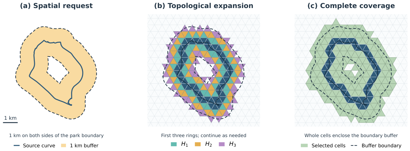
Figure 2.
Topological construction of the first two halo rings. The yellow seed ring is . Expanding and excluding previously discovered cells produces the green immediate neighbor ring ; expanding the completed ring produces the light blue ring . Red overlays select seed cells on the left and cells of on the right, illustrating the current frontier in each expansion.
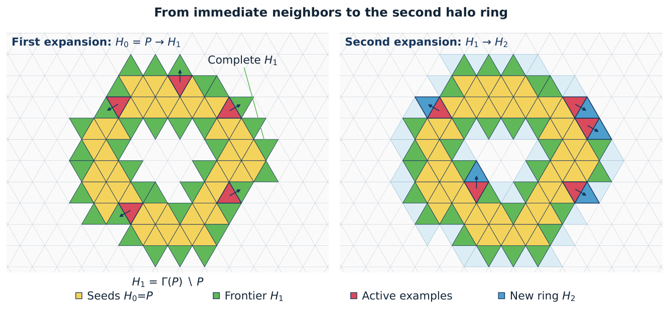
Figure 4.
Topological and spatial distance on a spherical triangular mesh. The dashed cell route can turn, whereas the orange great circle arc is the shortest spherical connection between the seed and target centroids. For a route of k adjacency steps, its length and the endpoint distance d satisfy , where is the maximum adjacent centroid distance at that resolution. The central angle determines the spherical endpoint distance , with in radians. The image is an annotated example (, ), not a measurement from the performance matrix.
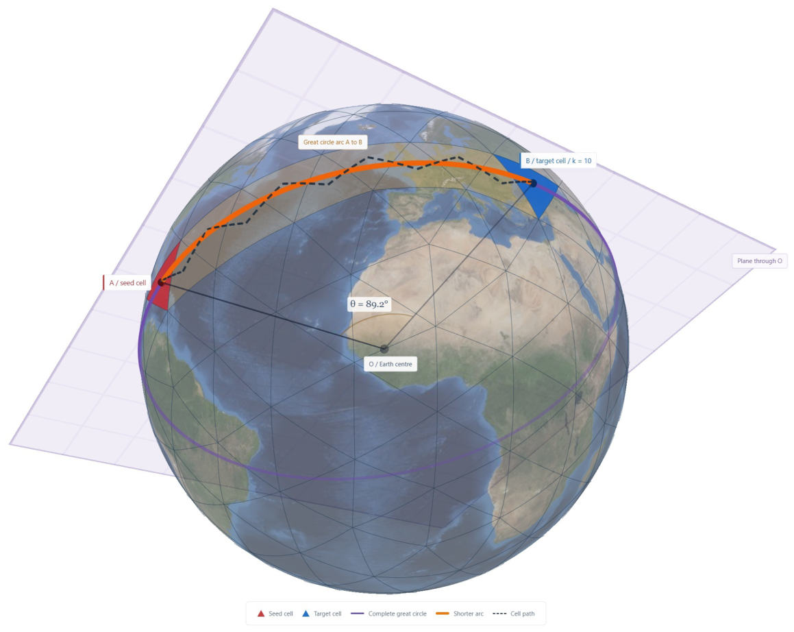
Figure 6.
Integer triangular coordinates on the chart of one base mesh face. The i axis follows the base mesh edge from vertex A toward B, the j axis follows the edge from A toward C, and the triangular grid contains upward cells and downward cells . The orientation bit o distinguishes the two cells associated with one integer grid position. The example uses , , and anchor ; this anchor identifies their coordinate bin and is not a vertex of both cells.
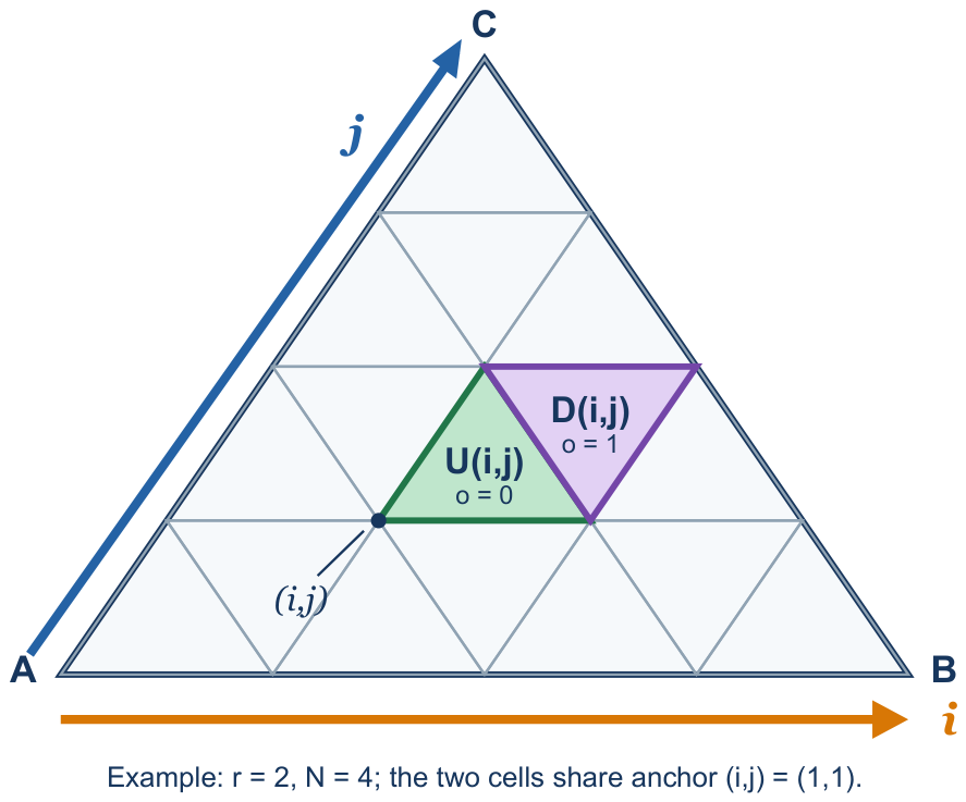
Figure 7.
Child digits for upward and downward parent cells. The three corner children retain the parent orientation; central child 3 has the opposite orientation. The digits refer to the public hierarchical index, not to the integer coordinates.
Figure 7.
Child digits for upward and downward parent cells. The three corner children retain the parent orientation; central child 3 has the opposite orientation. The digits refer to the public hierarchical index, not to the integer coordinates.
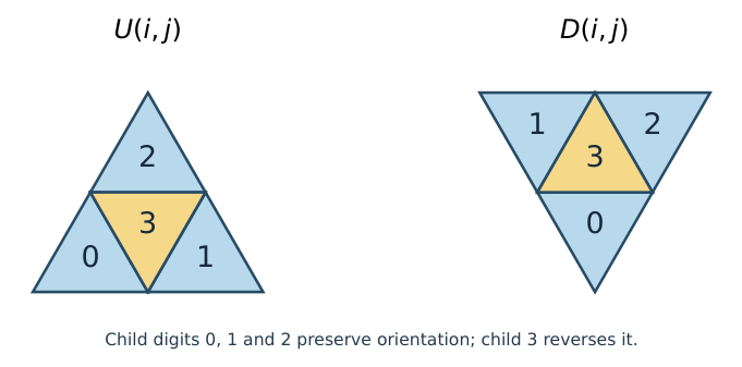
Figure 8.
Scientific comparison of the BIM index and the compact integer triangular index. (a) BIM’s symmetric three axis integer image is sparse: a syntactically valid triplet need not denote a cell. (b) Cross face BIM movement preserves one axis and swaps the other two according to the oriented edge pair. (c) The compact integer triangular index uses two chart coordinates and an explicit orientation bit; every tuple satisfying the triangular domain rule denotes one cell and interior neighbors follow fixed offsets. (d) For a base mesh edge crossing, t is the zero based position of the source boundary cell along source edge e, and is the corresponding position along destination edge . The illustrated transition from source edge 0 to destination edge 1 reverses positions to ; these values are local edge positions, not complete DGGS cell indices. Destination edge selects one of three boundary coordinate templates, reconstructing in the same 63 bit compact integer triangular index.
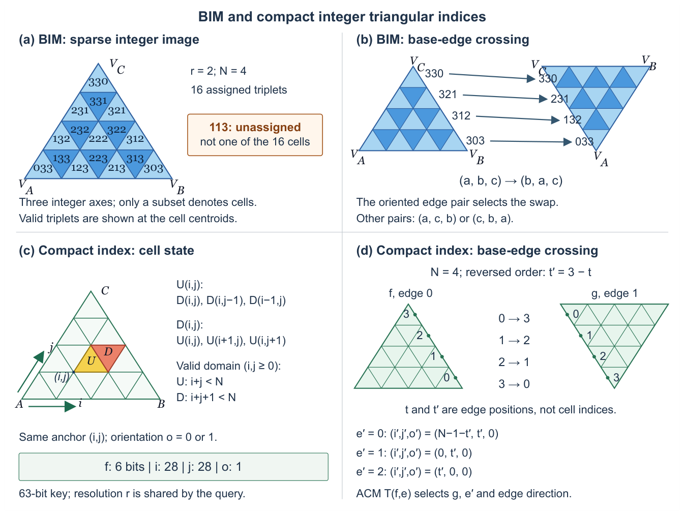
Figure 9.
Interior neighbors use Equations (11) and (12); only a base mesh boundary candidate reads a transition record. The same record applies at every refinement level.
Figure 9.
Interior neighbors use Equations (11) and (12); only a base mesh boundary candidate reads a transition record. The same record applies at every refinement level.
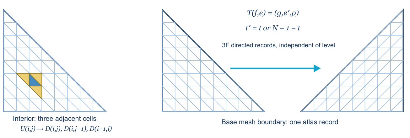
Figure 11.
Prepared Calgary point distributions. Buildings use representative footprint points, while streets and the boundary use regularly spaced line samples. The plots describe traversal inputs and do not imply exact polygon coverage.
Figure 11.
Prepared Calgary point distributions. Buildings use representative footprint points, while streets and the boundary use regularly spaced line samples. The plots describe traversal inputs and do not imply exact polygon coverage.
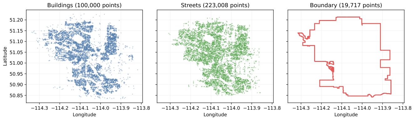
Figure 12.
Preindexed halo evaluation. (a) Faster flat CPU time divided by GPU pinned host readiness for all 81 selected session configurations, plotted against realized output. (b) Controlled variants on the largest query, each divided by the GPU implementation reference of its own session (architectural alternatives from the architectural variant session, mechanism removals from the mechanism removal session); the final row removes all four mechanisms together. (c) CPU thread scaling on the largest query; the one thread flat point is the serial implementation, and the GPU reference is its primary selected median. (d) Measured stage means from the mechanism removal session, with the returned container copy shown hatched outside pinned host readiness. The panels have distinct aggregation and timing scopes as stated in the text.
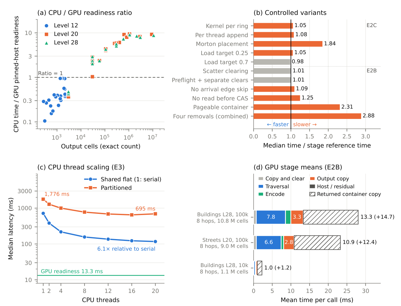
Figure 13.
Actual Pentakis cell sets for a 1 km WGS84 buffer of the complete Nose Hill Park boundary. The black curve is the source and the blue triangles are all returned cells: 78 at level 12 and 941 at level 14. The buffer extends to both sides of the boundary. The local projection is used only to display the result, not to determine cell membership.
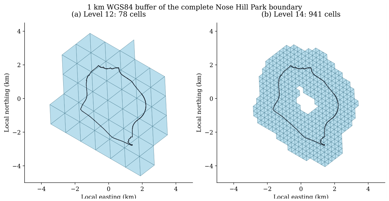
Table 1.
One refinement step in the public hierarchical index. Coordinates are expressed at the child’s resolution. Four applications of this table are composed into one conversion lookup.
Table 1.
One refinement step in the public hierarchical index. Coordinates are expressed at the child’s resolution. Four applications of this table are composed into one conversion lookup.
| Parent orientation | Child digit | Child |
|---|---|---|
| U | 0 | |
| U | 1 | |
| U | 2 | |
| U | 3 | |
| D | 0 | |
| D | 1 | |
| D | 2 | |
| D | 3 |
Table 3.
Boundary cell templates. The source template determines t; the ACM optionally reverses it. The destination template reconstructs the full cell on face g.
Table 3.
Boundary cell templates. The source template determines t; the ACM optionally reverses it. The destination template reconstructs the full cell on face g.
| Edge | Source boundary condition | Position | Destination |
|---|---|---|---|
| 0 | |||
| 1 | |||
| 2 |
Table 4.
Conservative surplus width for a 10 km request on the verified Pentakis mesh. Values are rounded upward. The distance interval width must be added to the last two distance columns. These are conditional spherical geometric bounds assuming valid source covering and distance intervals, not a certified floating point WGS84 result or measurements of a particular boundary query.
| Level | Cell radius bound (m) | Surplus (m) | Maximum retained distance (m) |
|---|---|---|---|
| 20 | 2.673382 | 5.346764 | 10005.346764 |
| 28 | 0.010443 | 0.020886 | 10000.020886 |
Table 5.
Calgary source and prepared traversal distributions.
| Dataset | Source records | Prepared points | Structure |
|---|---|---|---|
| Buildings | 511,586 | 100,000 | clustered |
| Streets | 120,008 | 223,008 | network like |
| Boundary | 1 | 19,717 | long curve |
Table 6.
Timing boundaries. Readiness in an internal pinned buffer differs from returning a newly owned container. Point mapping includes sorting and duplicate removal; file operations and source covering are excluded here.
Table 6.
Timing boundaries. Readiness in an internal pinned buffer differs from returning a newly owned container. Point mapping includes sorting and duplicate removal; file operations and source covering are excluded here.
| Scope | Included work | Interpretation |
|---|---|---|
| Device pipeline | Input transfer, initialization, seed decoding and expansion, final control and offset readback, output encoding | CUDA event interval; excludes bulk cell array download |
| Pinned host readiness | Device pipeline and transfer to the retained pinned host buffer | Primary GPU timer; returned vector copy excluded |
| Returned container completion | Readiness plus allocation and copy into returned vector | Separately timed stages; no direct distribution of their summed call latency |
| CPU returned output | CPU traversal, conversion, and returned vector construction | Primary CPU timer |
| Mapping inclusive view | One measured mapping stage plus selected halo latency | Reconstructed workflow estimate; not geometry covering |
Table 7.
Latencies by realized output size, in milliseconds. Latency columns are group medians of the selected eligible session medians defined in Section 3.6.4. CPU timings include a fresh returned container; GPU timings end at pinned host readiness, before its returned container copy. Ratio is the faster serial or twenty thread flat CPU time divided by GPU readiness for each configuration; its group median is not the ratio of marginal median times. CPU and GPU sessions are selected independently. The lower endpoint of each interval after the first is excluded.
| Output cells | Conf. | Serial flat | Twenty thread flat | GPU | Ratio | Range | GPU faster |
|---|---|---|---|---|---|---|---|
| up to 3 000 | 33 | 0.0619 | 0.123 | 0.162 | 0.37 | 0.10 to 0.95 | 0 of 33 |
| 3 000 to 40 000 | 12 | 0.793 | 0.472 | 0.201 | 2.46 | 1.03 to 2.94 | 12 of 12 |
| 40 000 to 120 000 | 8 | 3.17 | 1.38 | 0.329 | 4.14 | 2.37 to 4.37 | 8 of 8 |
| 120 000 to 400 000 | 10 | 9.48 | 1.98 | 0.354 | 5.49 | 5.10 to 5.88 | 10 of 10 |
| 0.4 to 1.2 million | 9 | 55.1 | 8.76 | 0.943 | 9.10 | 6.08 to 9.45 | 9 of 9 |
| 1.2 to 4 million | 5 | 153 | 26.2 | 3.13 | 8.20 | 7.95 to 8.51 | 5 of 5 |
| 4 to 11 million | 4 | 662 | 109 | 12.2 | 8.93 | 8.79 to 9.25 | 4 of 4 |
| all | 81 | – | – | – | 2.38 | 0.10 to 9.45 | 48 of 81 |
Table 8.
Selected session ratios by dataset, with 27 configurations per dataset. Each ratio compares the faster flat CPU implementation with GPU pinned host readiness. Timing ownership and independent session selection are as in Table 7.
Table 8.
Selected session ratios by dataset, with 27 configurations per dataset. Each ratio compares the faster flat CPU implementation with GPU pinned host readiness. Timing ownership and independent session selection are as in Table 7.
| Dataset | Median | Minimum | Maximum | GPU faster |
|---|---|---|---|---|
| Buildings | 2.56 | 0.15 | 9.45 | 16 of 27 |
| Streets | 2.83 | 0.18 | 9.44 | 16 of 27 |
| Boundary | 2.37 | 0.10 | 9.24 | 16 of 27 |
Table 9.
Representative configurations from the primary summary. All queries use eight hops. All times are selected eligible session medians in milliseconds. GPU is pinned host readiness, not full returned container latency. References count three logical neighbor constructions per expanded cell, including the arrival neighbors subsequently skipped before lookup. Lr denotes level r; 10k and 100k in the Query column denote requested point counts, not necessarily unique seed counts after mapping. The Unique seeds column gives the actual count. Later stage tables use actual seed counts; shorthand point categories in Figure 12 identify the same configurations.
| Dataset | Query | Unique seeds | Output cells | Logical references |
Serial flat | Twenty thread flat |
GPU |
|---|---|---|---|---|---|---|---|
| Buildings | L28, 10k | 10,000 | 1,080,000 | 2,550,000 | 56.3 | 9.09 | 1.01 |
| Streets | L20, 100k | 99,657 | 9,010,953 | 22,253,169 | 595 | 100 | 10.8 |
| Buildings | L28, 100k | 100,000 | 10,800,000 | 25,500,000 | 715 | 117 | 13.3 |
| Boundary | L28, all | 19,717 | 2,129,436 | 5,027,835 | 126 | 20.9 | 2.46 |
Table 10.
CPU thread scaling from one measurement session, in milliseconds. Parallel columns are medians of thirty calls. The one thread reference aggregates serial flat medians across the sweep invocations; columns 2 through 20 use the multithreaded flat table. Ratio compares the one thread and twenty thread times. The final column retains the partitioned implementation as a diagnostic. These measurements do not establish a hardware bottleneck or a scaling limit beyond twenty threads.
| Query | 1 (serial flat) |
2 | 4 | 8 | 12 | 16 | 20 | Ratio 1:20 |
Partitioned, 20 |
|---|---|---|---|---|---|---|---|---|---|
| Buildings L28, 100k seeds, 8 hops. |
716 | 382 | 218 | 157 | 136 | 123 | 117 | 6.1 | 695 |
| Streets L20, 100k seeds, 8 hops. |
597 | 322 | 314 | 124 | 110 | 104 | 98.1 | 6.1 | 544 |
| Buildings L28, 10k seeds, 8 hops. |
61.2 | 29.6 | 17.1 | 11.5 | 10.1 | 9.89 | 9.07 | 6.7 | 51.4 |
| Buildings L12, 1914 seeds, 4 hops. |
0.0679 | 0.0882 | 0.171 | 0.104 | 0.113 | 0.178 | 0.206 | 0.3 | 0.997 |
Table 11.
Schedule study of Section 3.6.2, as ratios of configuration means to the earlier GPU release. Values above one are slower. All variants use the same cell semantics; this reference is not the GPU implementation of the primary matrix. Macrochart sorting uses the rhombic macrocharts defined in Section 3.6.2.
| Workload | Host managed sets |
Triangle sorting |
Macrochart sorting |
|---|---|---|---|
| Compact, 100k seeds, 1 hop | 72.80 | 28.17 | 27.59 |
| Compact, 100k seeds, 4 hops | 51.19 | 21.08 | 21.25 |
| Compact, 100k seeds, 8 hops | 23.18 | 12.96 | 11.65 |
| Compact, 10k seeds, 4 hops | 18.25 | 19.41 | 21.23 |
| Scattered, 100k seeds, 4 hops | 126.16 | 46.46 | 47.20 |
| Base mesh boundary, 100k seeds, 4 hops | 45.61 | 18.17 | 19.25 |
Table 12.
Controlled variants relative to the GPU implementation. Reference medians are shown separately for the architectural variant session (E2C) and the mechanism removal session (E2B); every ratio uses its own session and query. Rows 1–6 and 13 use E2C, and rows 7–12 use E2B. Rows 8–11 remove individual mechanisms; row 11 bundles preflight and control clearing, and row 12 removes all four together. Thus not every row isolates one operation. Row 8 includes fresh container delivery rather than pinned readiness. A dash means no completed measurement is reported, not zero cost.
| Variant | Buildings L28 100k seeds, 8 hops | Streets L20 100k seeds, 8 hops | Buildings L28 10k seeds, 8 hops | Buildings L12 1914 seeds, 4 hops |
|---|---|---|---|---|
| Reference, architectural variant session (E2C), ms | 13.30 | 10.82 | 1.010 | 0.1657 |
| Reference, mechanism removal session (E2B), ms | 13.29 | 10.87 | 1.014 | 0.1431 |
| 1. Kernel launch per ring instead of one cooperative launch | 1.05 | 1.09 | 1.42 | 2.25 |
| 2. Per thread output counter instead of warp aggregated append | 1.08 | 1.07 | 1.16 | 1.02 |
| 3. Masked key instead of SplitMix mixing | – | – | – | 44.65 |
| 4. Block local Morton placement instead of SplitMix mixing | 1.84 | 3.45 | 2.79 | 0.97 |
| 5. Load target 0.25 instead of 0.5 | 1.05 | 1.07 | 1.35 | 0.97 |
| 6. Load target 0.7 instead of 0.5 | 0.98 | 0.96 | 0.96 | 0.96 |
| 7. Scatter clearing instead of full table clear | 1.01 | 1.00 | 1.00 | 1.04 |
| 8. Fresh pageable container instead of the pinned reusable buffer | 2.31 | 2.45 | 2.76 | 1.09 |
| 9. Without arrival edge skipping (three lookup candidates per frontier cell) | 1.09 | 1.09 | 0.99 | 1.55 |
| 10. Without the read before the compare and swap | 1.25 | 1.30 | 1.14 | 1.54 |
| 11. Memory preflight and separate control clears on every call | 1.01 | 1.02 | 1.07 | 1.13 |
| 12. Rows 8 to 11 together (without the four mechanisms) | 2.88 | 2.98 | 2.87 | 1.09 |
| 13. Output budget set to the realized output count instead of the automatic output budget | 1.00 | 1.00 | 1.00 | 1.06 |
Table 13.
Measured stage means over 30 calls in the mechanism removal session (E2B). All timing columns are in milliseconds; Output cells is a count. Copy and clear includes input transfer and device initialization; traversal includes seed decoding, expansion, final control and ring offset readback, and the intervening scheduling interval; encode converts output indices; output copy transfers to reusable pinned host memory. Ready is the instrumented pinned host readiness time, not the complete call. Container copy is the subsequent allocation and copy into the returned vector, outside that timer. Other contains host and residual timing. Small differences arise from printed rounding.
| Query | Output cells |
Copy and clear |
Traversal | Encode | Output copy |
Other | Ready | Container copy |
|---|---|---|---|---|---|---|---|---|
| Buildings L28, 100k seeds, 8 hops |
10 800 000 | 0.72 | 7.83 | 1.43 | 3.30 | 0.04 | 13.33 | 14.69 |
| Streets L20, 99,657 seeds, 8 hops |
9 010 953 | 0.74 | 6.64 | 0.69 | 2.76 | 0.05 | 10.88 | 12.37 |
| Buildings L28, 10k seeds, 8 hops |
1 080 000 | 0.09 | 0.37 | 0.20 | 0.34 | 0.02 | 1.01 | 1.23 |
| Buildings L12, 1914 seeds, 4 hops |
1 046 | 0.03 | 0.07 | 0.03 | 0.01 | 0.01 | 0.15 | 0.00 |
| Boundary L12, 287 seeds, 1 hop |
312 | 0.02 | 0.05 | 0.03 | 0.01 | 0.01 | 0.13 | 0.00 |
Table 14.
Measured means in the mechanism removal session (E2B) with and without the four mechanisms. All timing columns are in milliseconds; Ratio is dimensionless. Device includes initialization, traversal, and encoding. Allocation is the timed output container allocation and initialization, not a measurement of page faults. Without the four mechanisms, Total includes fresh pageable output. With them, Ready ends at pinned host readiness and Container copy is the post timer copy. The last column compares these different delivery boundaries; adding Ready and Container copy gives a closer container delivery comparison, but is a sum of stage means rather than a separately timed complete call.
| Without the four mechanisms | GPU implementation | ||||||||
|---|---|---|---|---|---|---|---|---|---|
| Query | Device | Copy | Allocation | Total | Device | Copy | Ready |
Container copy |
Ratio |
| Buildings L28, 100k seeds, 8 hops |
16.44 | 7.17 | 14.56 | 38.21 | 9.98 | 3.30 | 13.33 | 14.69 | 2.87 |
| Streets L20, 99,657 seeds, 8 hops |
14.03 | 5.46 | 12.92 | 32.45 | 8.06 | 2.76 | 10.88 | 12.37 | 2.98 |
| Buildings L28, 10k seeds, 8 hops |
0.82 | 0.70 | 1.37 | 2.91 | 0.66 | 0.34 | 1.01 | 1.23 | 2.87 |
| Buildings L12, 1914 seeds, 4 hops |
0.13 | 0.01 | 0.00 | 0.16 | 0.13 | 0.01 | 0.15 | 0.00 | 1.06 |
| Boundary L12, 287 seeds, 1 hop |
0.14 | 0.01 | 0.00 | 0.16 | 0.11 | 0.01 | 0.13 | 0.00 | 1.24 |
Table 15.
Median boundary query computation times over three fresh process runs. CPU and hybrid query times include source covering and footprint filtering; hybrid time also includes GPU initialization. Validation and output file writing are excluded. Expansion is the sum of GPU expansion and hashing times across all replay calls, not the complete query time.
| Source and level | Distance (m) | Cells | Last ring | CPU (ms) | Hybrid (ms) | Expansion (ms) |
|---|---|---|---|---|---|---|
| Nose Hill, 12 | 1000 | 78 | 4 | 30.09 | 110.92 | 0.126 |
| Nose Hill, 14 | 1000 | 941 | 16 | 95.69 | 168.51 | 0.219 |
| Nose Hill, 16 | 1000 | 13,874 | 64 | 618.59 | 754.01 | 0.810 |
| Point, 20 | 10 | 60 | 8 | 1.29 | 87.86 | 0.135 |
| Point, 28 | 0.1 | 316 | 32 | 2.50 | 84.78 | 0.357 |
| Date line, 12 | 1000 | 14 | 4 | 1.70 | 83.04 | 0.097 |
| Near pole, 12 | 1000 | 10 | 4 | 1.94 | 82.68 | 0.113 |
Table 17.
Direct specialization to triangular spherical base meshes.
| Base mesh | F | ACM records | Base mesh vertex valence |
|---|---|---|---|
| Pentakis dodecahedron | 60 | 180 | 5 and 6 |
| Icosahedron | 20 | 60 | 5 |
| Octahedron | 8 | 24 | 4 |
Disclaimer/Publisher’s Note: The statements, opinions and data contained in all publications are solely those of the individual author(s) and contributor(s) and not of MDPI and/or the editor(s). MDPI and/or the editor(s) disclaim responsibility for any injury to people or property resulting from any ideas, methods, instructions or products referred to in the content. |
© 2026 by the authors. Licensee MDPI, Basel, Switzerland. This article is an open access article distributed under the terms and conditions of the Creative Commons Attribution (CC BY) license (http://creativecommons.org/licenses/by/4.0/).
Copyright: This open access article is published under a Creative Commons CC BY 4.0 license, which permit the free download, distribution, and reuse, provided that the author and preprint are cited in any reuse.