

Submitted:
19 October 2026
Posted:
20 October 2026
You are already at the latest version
Abstract
This paper asks which type of political behaviour drives spatial interdependence in municipal spending. Under yardstick competition, voters benchmark their incumbent against neighbouring jurisdictions, but the literature offers two opposite predictions about who mimics most: the swing voter hypothesis predicts that electorally vulnerable incumbents mimic more, while the core voter hypothesis predicts that politically strong incumbents mimic more. I extend the yardstick competition model to allow the spatial autoregressive parameter to vary across regimes defined by two dimensions of political strength, horizontal electoral concentration and vertical alignment with the federal president and the state governor, and take the predictions to a panel of 857-940 Mexican municipalities over 2001-2021 using regime-switching spatial Durbin models estimated by quasi-maximum likelihood with time-varying Jacobians. When political strength is measured by electoral concentration, politically weak mayors mimic around 60 percent more than strong ones, supporting the swing voter hypothesis. When it is measured by vertical alignment, aligned mayors mimic significantly more, supporting the core voter hypothesis. Four-regime specifications reveal an asymmetry: national alignment combined with concentration reinforces the core voter pattern, regional alignment combined with concentration reverses the concentration effect, and the joint combination of both vertical alignments restores the swing voter pattern. The two mechanisms are not mutually exclusive but operate along different dimensions of political strength.
Keywords:
yardstick competition
; fiscal mimicking
; spatial Durbin model
; regime switching
; political alignment
; Mexican municipalities
1. Introduction
What type of political behaviour drives spatial interdependencies in Mexican municipal expenditures? Moreno Jimenez (2026b) establishes the existence of significant public expenditure spillovers among Mexican municipalities. Having confirmed that municipalities do not operate in fiscal isolation, the natural progression of this research is to identify the political mechanisms driving these interactions. The political economy literature offers two competing hypotheses. The swing voter hypothesis, grounded in the work of Lindbeck and Weibull (1987) and Dixit and Londregan (1996), posits that electoral insecurity drives mimicking: vulnerable incumbents copy their neighbours to appease undecided voters who use neighbouring jurisdictions as benchmarks. The core voter hypothesis, associated with Cox and McCubbins (1986), suggests the opposite: politically strong incumbents mimic to maintain their core constituency and minimise the risks of policy innovation. This paper tests which mechanism predominates in Mexican municipal fiscal behaviour.
The Mexican context offers a particularly rich setting for this inquiry. As argued by Moreno Jimenez and Ramírez Casillas (2022), political actors in Mexico operate under conditions of high risk aversion, where the primary objective is often regime maintenance rather than electoral expansion. Moreover, Mexican municipalities are embedded in a complex web of vertical intergovernmental relations. Receiving approximately 90 percent of their revenue from federal and state transfers, local incumbents must navigate relationships with both the Federal President and the State Governor. This dual dependency creates multiple dimensions of political strength: an incumbent may be electorally secure but vertically isolated, or electorally vulnerable but federally connected. As I demonstrate in this paper, the answer to which dimension drives horizontal mimicking is not singular: electoral concentration triggers swing voter behaviour, while vertical alignment triggers core voter behaviour. The two mechanisms are not mutually exclusive but operate along different dimensions of political strength, with the interaction between them producing patterns that neither pure hypothesis anticipates.
I address this complexity by extending the spatial regime framework proposed by Elhorst and Fréret (2009). First, I estimate two-regime specifications to isolate the individual effects of three dimensions of political strength: local electoral concentration, national alignment (with the President), and regional alignment (with the Governor). This stage reveals whether each dimension independently supports the swing voter or core voter hypothesis. Second, I extend to four-regime specifications that interact electoral concentration with vertical alignments. This progression allows me to test whether the swing voter and core voter mechanisms operate along different dimensions of political strength, and to examine how vertical alignment moderates the relationship between electoral concentration and horizontal mimicking.
The empirical results reveal a pattern that cannot be fully explained by either hypothesis alone. When political strength is measured by electoral concentration, the swing voter hypothesis receives support since politically vulnerable mayors mimic more intensely. When vertical alignment is introduced, the core voter hypothesis dominates since politically connected mayors exhibit stronger spatial interactions. The four-regime specifications show that the relationship between political strength and mimicking depends on which dimensions are interacted. On the one hand, national alignment combined with electoral concentration supports the core voter logic; on the other hand, regional alignment combined with electoral concentration reverses the concentration effect. Finally, the joint consideration of both vertical alignments restores the swing voter pattern.
These findings contribute to the literature in three ways. First, on the methodological side, I combine two-regime and four-regime spatial specifications to disentangle a politically complex system in which electoral concentration, national alignment, and regional alignment operate as distinct dimensions of political strength. Second, on the theoretical side, I extend the yardstick competition framework to accommodate both the swing voter and the core voter logics within a single estimable model. Rather than treating these hypotheses as competing predictions over a single dimension of political strength, I show that they coexist along different dimensions. Third, on the empirical side, I extend Elhorst and Fréret (2009) to a Latin American federal system using a recent and large municipal panel for Mexico (2001–2021), providing new evidence on a region where studies on horizontal fiscal interactions remain scarce.
The remainder of this paper is organised as follows. Section 2 describes the institutional background and political context, documenting the patterns of political concentration and alignment in Mexican municipalities. Section 3 reviews the literature on horizontal fiscal interactions, situating the Mexican case within the yardstick competition framework and contrasting the swing voter and core voter predictions. Section 4 presents the empirical strategy, developing the theoretical framework that derives heterogeneous reaction functions from a yardstick competition model and outlining the two-regime and four-regime Spatial Durbin Models and the quasi-maximum likelihood estimation technique. Section 5 presents the empirical results, analysing the heterogeneity in spatial interactions across two-regime and four-regime specifications, including difference-in-differences analysis, robustness checks, and sensitivity analyses. Section 6 offers concluding remarks and discusses the implications for the design of intergovernmental fiscal relations in Mexico. Appendix A reports the full estimation results for all specifications and spatial weight matrices.
2. Institutional Background and Political Context
As highlighted in Moreno Jimenez and Ramírez Casillas (2022), budgetary dynamics in Mexico incorporate not only economic components but also significant political dimensions. The study demonstrates that higher levels of fund discretion strengthen the political component in fiscal allocations. Building on this foundation, this paper examines how two key political variables influence municipal finance: political concentration and political alignment.
Following Moreno Jimenez (2026b), political concentration is measured as the percentage of votes obtained by the municipal president and their political party in local elections. This indicator captures the degree of electoral dominance within municipalities, reflecting the consolidation of political power at the local level. Figure 1 illustrates the temporal evolution of political concentration from 2001 to 2021. While there has been a gradual decline in political concentration over this period, the decrease has been moderate, with averages shifting from 0.48 in 2001 to 0.40 in 2021. The spatial distribution of political concentration, shown in Figure 2, reveals considerable heterogeneity across Mexican municipalities, indicating regional variations in electoral competition and party dominance.
Moreno Jimenez (2026b) examined political alignment solely as the relationship between municipal presidents and the federal president, operationalised as a binary variable equal to one when both belong to the same political party and zero otherwise. This paper expands this conceptualisation by introducing regional alignment as an additional dimension of vertical political relationships. Regional alignment is measured as another binary variable equal to 1 when the municipal president (second subnational level) shares political affiliation with the state governor (first subnational level), and 0 otherwise. This dual alignment framework acknowledges the complex vertical political relationships that characterise Mexican federalism. As Moreno Jimenez and Ramírez Casillas (2022) argues, fiscal federalism in Mexico inherently incorporates political dimensions that influence intergovernmental transfers and resource allocation.
The relevance of analysing both federal and state-level political alignments stems from the structure of municipal financing in Mexico. Municipalities receive unconditional transfers from both federal and state governments in comparable proportions, as shown in Figure 3. This dual dependency creates a challenging political environment for municipal presidents, who must navigate relationships with both federal and state authorities while managing local fiscal affairs.
Figure 4 presents the temporal evolution of national and regional alignment averages. The graph reveals distinct patterns: from 2001 to 2012, regional alignment consistently exceeded national alignment. From 2013 onward, these alignment measures have converged, suggesting changing political dynamics across government levels.
The spatial patterns of political alignments are shown in Figure 5 and Figure 6, which demonstrate substantial geographical heterogeneity in political affiliations across Mexico’s municipalities.
To better understand the intersection of these political relationships, I constructed a categorical variable combining both national and regional alignment dimensions. This classification creates four distinct categories of municipal presidents: aligned only with the governor, aligned only with the president, aligned with both, or aligned with neither.
Figure 7 traces the evolution of these categories over time, revealing several important trends: alignment with neither level of government has increased, alignment with governors has decreased, alignment with presidents has remained relatively constant, and alignment with both reached a peak between 2013 and 2017.
The geographical prevalence of these alignment patterns is shown in Figure 8, where again substantial heterogeneity is evident, particularly considering that northern municipalities in Mexico tend to be larger both in area and population.
The statistical distribution of municipal alignment patterns provides further insight into these political dynamics. Table 1 presents both the overall distribution (2001–2021) and the evolution across four distinct periods.
Several important patterns emerge from this statistical summary. First, over the entire 2001–2021 period, “Neither” represents the most common category (37.7%), followed by “Governor Only” (30.7%), “President Only” (19.2%), and “Both” (12.3%).
The temporal evolution reveals significant shifts in alignment patterns. During 2001–2005, alignment patterns were relatively balanced between “Neither” (36.8%) and “Governor Only” (36.7%). The 2006–2011 period saw a notable increase in “Governor Only” alignment (42.9%), while “Neither” alignment decreased to 29.4%. The 2012–2017 period marked a substantial shift, with “Aligned with Both” reaching its peak (24.1%) and “Governor Only” alignment declining sharply to 20.6%. Most strikingly, the 2018–2021 period shows a dramatic increase in “Aligned with Neither” municipalities (55.8%) and a corresponding decline in “Aligned with Both” (3.6%), suggesting increasing political fragmentation or divergence between municipal, state, and federal levels.
These statistical patterns corroborate the visual evidence presented in Figure 7 and Figure 8, confirming that political alignment in Mexican municipalities is not only heterogeneous across space but has also undergone significant temporal transformations, particularly following major political realignments at the national level.
This institutional and political context establishes the foundation for understanding how vertical political relationships between municipal, state, and federal governments interact with fiscal allocation mechanisms in Mexico. The complexity revealed by these descriptive analyses underscores the importance of considering multiple dimensions of political alignment when examining municipal finance in a federal system characterised by complex intergovernmental relations.
3. Literature Review
While Moreno Jimenez (2026b) focused on identifying the presence of expenditure spillovers, this paper focuses on yardstick competition and, crucially, on identifying which type of political behaviour drives it. As delineated in the seminal work of Besley and Case (1995), yardstick competition posits that in a world of imperfect information, voters face a signal extraction problem regarding the quality of their incumbents. Voters observe taxes and public services but cannot directly assess government efficiency. Consequently, they use the fiscal performance of neighbouring jurisdictions as a benchmark. If neighbours provide better services or lower taxes under similar conditions, voters infer that their own government is inefficient or rent-seeking. This benchmarking behaviour forces rational incumbents to mimic the fiscal policies of their neighbours to avoid electoral punishment.
While the yardstick competition framework explains why mimicking occurs, it does not unambiguously predict which incumbents are most prone to this behaviour. The literature offers two competing hypotheses that yield opposite empirical predictions. The swing voter hypothesis, grounded in the work of Lindbeck and Weibull (1987) and Dixit and Londregan (1996), views elections as a competition for pivotal, ideologically neutral voters. Under this framework, yardstick competition is primarily a survival strategy: politically insecure incumbents, facing tight electoral margins, are the most likely to mimic neighbours because they cannot afford to appear less competent than nearby jurisdictions. A mayor with a comfortable electoral majority has less to fear from voter comparisons; a vulnerable mayor risks losing office if voters perceive better performance elsewhere. This logic predicts that spatial interaction intensity should be higher among politically weak incumbents than among strong ones.
The core voter hypothesis, associated with Cox and McCubbins (1986), offers a competing prediction. Originally formulated in the context of distributive politics, this model views elections as a redistributive game where risk-averse politicians prefer to invest in their loyal support base rather than court uncertain swing voters. Cox and McCubbins (1986) argue that targeting core supporters yields more predictable electoral returns than the gamble of persuading undecided voters. While this framework was developed to explain the allocation of transfers rather than spatial mimicking, its logic extends naturally to horizontal fiscal interactions. If incumbents are risk-averse, policy innovation carries electoral risk: a novel policy might succeed and attract new supporters, but it might also fail and alienate existing ones. Mimicking neighbours, by contrast, reduces this variance because if the policy fails, it fails everywhere, diffusing blame; if it succeeds, the incumbent shares in the regional success. Further, only incumbents with sufficient political capital can sustain such coordinated behaviour without losing their base. This logic is the opposite of the swing voter one because it predicts that spatial interaction intensity should be higher among politically strong incumbents than among weak ones.
The core voter logic is particularly relevant for the Mexican case. Moreno Jimenez and Ramírez Casillas (2022) document that political actors in Mexico exhibit significant risk aversion, prioritising the maintenance of established power structures over the uncertainty of electoral expansion. In their analysis of Mexican governors’ fiscal behaviour, they find that incumbents systematically avoid policies that might destabilise their political position, even when such policies might yield electoral gains. This behavioural pattern aligns closely with the core voter framework. If Mexican municipal presidents exhibit similar risk aversion, they would be more likely to engage in coordinated mimicking when they possess the political strength to sustain it, rather than when electoral vulnerability forces them to innovate. This insight suggests that the standard yardstick competition prediction, that vulnerability drives mimicking, may not hold in institutional contexts characterised by risk-averse political actors. Instead, fiscal mimicking may function as a regime maintenance strategy, where strong incumbents synchronise policy to consolidate their position, rather than a survival strategy where weak incumbents copy neighbours to avoid removal.
A limitation of the existing literature is its treatment of political strength as a unidimensional concept, typically operationalised through electoral margins or vote shares. However, in federal systems with significant intergovernmental fiscal relationships, political strength has multiple dimensions that may not move together. Consider a municipal president in Mexico. Her political strength depends not only on her local electoral margin (horizontal dimension) but also on her alignment with higher levels of government (vertical dimension). A mayor may enjoy a commanding electoral majority but face an opposition governor who controls discretionary transfers. Conversely, a mayor with a narrow electoral margin may be aligned with both the president and the governor, providing access to resources and political protection. These two mayors occupy different positions in the multidimensional space of political strength, and their incentives for horizontal mimicking may differ accordingly. This multidimensionality raises the possibility that the swing voter and core voter mechanisms are not mutually exclusive but operate along different dimensions. Electoral concentration, which captures local vulnerability, may trigger swing voter behaviour: mayors facing tight races mimic to appease undecided voters. Vertical alignment, which captures access to higher-level resources and political protection, may trigger core voter behaviour: connected mayors mimic to coordinate the deployment of intergovernmental transfers and maintain their support base. If this is the case, the empirical pattern would depend on which dimension of political strength is examined.
The relationship between vertical alignment and horizontal mimicking merits particular attention. Mexican municipalities depend on federal and state transfers for approximately 90 percent of their revenue, creating a dual vertical dependency. As Keen (1998) emphasises, fiscal interactions in federations occur not only horizontally among jurisdictions at the same level but also vertically between tiers of government. This vertical dimension can affect horizontal behaviour in several ways.
First, vertical alignment may reduce horizontal mimicking. A mayor aligned with the governor has access to discretionary resources and political protection that reduce the need to coordinate with neighbours. If fiscal mimicking serves as a strategy to reduce electoral risk, vertical alignment provides an alternative risk-reduction mechanism, predicting that aligned mayors mimic less than non-aligned ones.
Second, vertical alignment may increase horizontal mimicking. A mayor aligned with higher levels of government may use horizontal mimicking to maximise the collective political returns of intergovernmental transfers. If the governor channels resources to aligned municipalities, these municipalities may coordinate their spending to amplify the electoral impact across the region, predicting that aligned mayors mimic more than non-aligned ones.
Third, the relationship may depend on the level of vertical alignment. Alignment with the federal president connects municipalities directly to national resources but may skip state-level intermediaries. Alignment with the state governor provides access to state-mediated transfers and regional political networks. Municipalities aligned with one level but not the other face a partial vertical connection that may induce different horizontal behaviour. This asymmetry suggests that national and regional alignment may have different effects on horizontal mimicking. Which pattern prevails is ultimately an empirical question.
Empirically distinguishing between these mechanisms presents significant challenges. The reflection problem identified by Manski (1993) implies that standard spatial econometric techniques can identify spatial correlation but cannot easily distinguish whether this correlation arises from spillover effects, common shocks, or strategic political interaction. A substantial portion of the literature has attempted to resolve this simultaneity using Instrumental Variable (IV) estimation. However, Elhorst and Fréret (2009) provide a compelling critique of the IV approach in this context. They argue that while IV estimators are popular, they risk producing spatial coefficient estimates outside the valid parameter space. Unlike Quasi-Maximum Likelihood (QML) estimators, IV estimators ignore the Jacobian term in the log-likelihood function, which restricts the spatial coefficient to an interval defined by the eigenvalues of the spatial weight matrix.
Furthermore, identifying valid instruments that affect neighbours’ spending but not local spending is notoriously difficult in fiscal policy contexts. To address these limitations, I follow the strategy proposed by Elhorst and Fréret (2009), who argue that yardstick competition implies a regime-dependent spatial relationship. If mimicking is driven by electoral concerns, its intensity should vary systematically with political characteristics. By employing a Spatial Durbin Model (SDM) with regime-switching capabilities, I can test whether the spatial autoregressive parameter varies significantly across political regimes. This approach avoids the pitfalls of IV estimation by using Maximum Likelihood to estimate regime-specific spatial coefficients, allowing for a direct test of the competing theoretical predictions. Crucially, the regime-switching framework can accommodate the multidimensionality of political strength. By defining regimes based on different dimensions (electoral concentration, national alignment, regional alignment, and their interactions) I can test whether the swing voter and core voter mechanisms operate along different dimensions, and whether vertical alignment increases or decreases horizontal mimicking.
4. Empirical Strategy
4.1. Theoretical Framework
Following Case (1993), consider an incumbent who maximises utility U by choosing a level of public expenditure g and taxation :
where Y denotes taxpayer income and represents rents. The term captures the probability of reelection, and is the discount factor applied to future payoffs. The incumbent receives rents today and, if reelected with probability , receives discounted rents tomorrow.
Voters face an information asymmetry: they observe expenditures and taxes but cannot directly assess whether the incumbent is efficient or rent-seeking (Besley and Case 1995). Consequently, voters use neighbouring jurisdictions as a benchmark. This generates the following properties of the reelection function:
The derivative captures the yardstick effect: neighbours’ spending increases raise voter expectations, reducing the incumbent’s relative position and reelection odds.
The first-order condition for expenditure is:
The first term represents the marginal benefit of increasing g: higher reelection probability applied to future rents. The second term captures the marginal cost: one unit of rent lost today plus one unit of expected future rent forgone. This condition implicitly defines optimal expenditure as a function of neighbours’ policies.
Applying the implicit function theorem:
The denominator is negative by the second-order condition. The numerator is:
The second term, , is unambiguously positive. For the first term, I assume strategic complementarity in the reelection function: . This assumption reflects the yardstick logic: the marginal electoral return to own expenditure increases when neighbours spend more, because voters perceive higher spending as more justifiable. Under this assumption, the numerator is positive, implying : incumbents respond positively to neighbours’ expenditure changes. This reaction function corresponds to the spatial autoregressive coefficient in the empirical model.
The key insight for political yardstick competition is that the sensitivity of the reelection probability to neighbours’ policies varies with political characteristics. Let denote the political strength of incumbent i, where higher values indicate greater electoral security. I assume:
Under the standard yardstick competition hypothesis (Besley and Case 1995,Lindbeck and Weibull 1987), politically vulnerable incumbents are more sensitive to relative performance:
Incumbents with weak political positions face greater electoral pressure from swing voters who actively compare jurisdictions. This implies that the reaction function is decreasing in political strength:
However, an alternative prediction emerges from the core voter logic of Cox and McCubbins (1986). While the original model focuses on the efficient targeting of transfers to loyal supporters, the underlying intuition is that politicians may prioritise their secure base over uncertain swing voters, extending to fiscal coordination behaviour. If incumbents are risk-averse, they may prefer strategies that minimise variance in political payoffs rather than maximise expected gains from swing voter conversion. Consider an incumbent with utility , where represents political payoffs and is the coefficient of risk aversion. If policy deviations from neighbours increase variance (due to voter uncertainty or the political costs of appearing out of step with regional trends) risk-averse incumbents will coordinate more intensively. Crucially, only incumbents with sufficient political capital can effectively sustain synchronised policies, as coordination requires the stability and resources that come with electoral security. This generates the opposite prediction:
The theoretical framework generates two competing predictions regarding the relationship between political strength and spatial interaction intensity. Let denote political strength, where higher values indicate greater electoral security.
The swing voter hypothesis predicts that politically weak incumbents exhibit stronger mimicking behaviour:
The core voter hypothesis predicts the opposite pattern:
The following subsection develops a regime-switching spatial Durbin model that maps these theoretical predictions to an estimable empirical framework, allowing me to test which hypothesis better characterises fiscal interactions among Mexican municipalities.
4.2. Empirical Models
The empirical analysis employs the municipal panel constructed in Moreno Jimenez (2026a), covering the period 2001–2021. The baseline sample consists of a balanced panel of 857-940 municipalities (N depending on the specification). The only addition is the regional alignment variable described in Section 2, which reduces the sample to 857 municipalities (17,997 observations) due to missing values.
The theoretical framework developed in the previous subsection implies that the spatial autoregressive coefficient captures the average reaction , and that this coefficient should vary systematically with political strength . To test these predictions empirically, I specify a spatial panel data model with regime-switching capabilities, incorporating spatial and time-period fixed effects following the framework of Elhorst and Fréret (2009). The specification estimates a Spatial Durbin Model (SDM) where the spatial autoregressive parameter is allowed to vary across R distinct political regimes:
In this equation, denotes the ln of Subsidies and Social Benefits expenditure per capita in municipality i at time t. The term represents a vector of control variables, while corresponds to the element of the spatial weight matrix W.1 The coefficients and represent the individual spatial and time-period fixed effects, respectively, while is the error term. Let denote the set of observations belonging to regime r. The regime indicator variable is defined as:
such that for all , where R denotes the total number of regimes. Consequently, captures the specific intensity of spatial interaction for regime r, corresponding to the theoretical reaction function for municipalities in that regime. For all specifications, I test whether the spatial parameters differ significantly across regimes. Following Elhorst and Fréret (2009), I report pairwise differences between regime-specific coefficients with their t-statistics.
I implement this framework in two stages. First, I estimate two-regime specifications () to isolate the individual effects of political concentration, national alignment, and regional alignment. Second, I extend to four-regime specifications () to capture the interaction between political concentration and vertical alignments.
4.2.1. Two-Regime Specifications
I first estimate three two-regime specifications.
For Political Concentration ():
where denotes the q-th percentile of the distribution, with . Since higher political concentration implies greater electoral security, this specification orders political strength as .
For National Alignment ():
Since alignment with the federal president provides access to resources and political protection, this specification orders political strength as .
For Regional Alignment ():
Since alignment with the state governor provides similar political advantages, this specification also orders political strength as .
For the three cases, the swing voter hypothesis predicts , while the core voter hypothesis predicts .
4.2.2. Four-Regime Specifications
To examine the interactive effects of multiple political dimensions, I extend the framework to four-regime specifications. I assume that both dimensions contribute positively to political strength, so that for any two regimes r and , I define if regime r is weaker in at least one dimension and no stronger in the other.
For Political Concentration with National Alignment:
where captures municipalities with low concentration and no national alignment; those with low concentration but national alignment; those with high concentration but no national alignment; and those with high concentration and national alignment. This partial ordering implies , , , , and unambiguously. The regimes and are not directly comparable since each is stronger in one dimension.
For Political Concentration with Regional Alignment:
where captures municipalities with low concentration and no regional alignment; those with low concentration but regional alignment; those with high concentration but no regional alignment; and those with high concentration and regional alignment. This partial ordering implies , , , , and unambiguously. The regimes and are not directly comparable since each is stronger in one dimension.
For Combined National and Regional Alignments:
where captures municipalities aligned with neither level of government; those aligned with the governor only; those aligned with the president only; and those aligned with both. This specification directly tests the patterns shown in Table 1. This partial ordering implies , , , , and unambiguously. The regimes and are not directly comparable since each is stronger in one dimension.
For the three cases, the swing voter hypothesis predicts , , , , and . The core voter hypothesis predicts the opposite inequalities.
For the four-regime specifications, I further decompose the spatial parameters into marginal effects and interaction effects. Define the effect of political concentration conditional on alignment status:
and the effect of alignment conditional on concentration level:
Under the swing voter hypothesis, higher political strength reduces spatial interaction, so I expect , , , and . Under the core voter hypothesis, the opposite signs are expected.
The difference-in-differences estimator:
tests whether the effect of one political dimension depends on the level of the other. A positive indicates that the effect of political concentration on horizontal mimicking is stronger among non-aligned municipalities than among aligned ones; equivalently, the effect of alignment is stronger under low concentration than under high concentration. Conversely, implies the opposite pattern. This linear restriction on the parameters from Equation (12) is evaluated using a Wald test.
4.2.3. Quasi-Maximum Likelihood Estimation
To estimate the parameters of the spatial regime models, I employ the Quasi-Maximum Likelihood (QML) estimator. As derived by Elhorst and Fréret (2009), the estimation of models with spatial interaction effects and endogenous regimes requires a specific formulation of the likelihood function to account for the simultaneity introduced by the spatially lagged dependent variables. Unlike Instrumental Variable (IV) estimators, which ignore the Jacobian term and may produce spatial coefficients outside their valid parameter space, the QML approach maximises the probability of observing the sample data given the model structure, ensuring consistency and efficiency.
Following Elhorst and Fréret (2009) and Lee (2004), the log-likelihood function for the spatial Durbin panel data model with fixed effects and spatial regimes is given by:
The second term on the right-hand side is the Jacobian of the transformation, which restricts the spatial parameters to a stable range. Here, is the identity matrix, and is a diagonal matrix whose elements equal 1 if the observation belongs to regime r at time t. Because the political regimes can vary over time (e.g., due to elections), this Jacobian must be evaluated for each time period t, distinguishing this approach from standard time-invariant spatial models.
To make the maximisation computationally feasible, I employ a concentration procedure. I first transform the data to eliminate the spatial () and time-period () fixed effects using a demeaning operator. Then, I concentrate the likelihood function with respect to the linear parameters , and the error variance . This reduces the optimisation problem to a numerical search over the spatial autoregressive parameters . Once the optimal values are found, the remaining parameters and their asymptotic standard errors are recovered using the information matrix, as detailed in Elhorst and Fréret (2009). All models are estimated in MATLAB R2024a (Update 3), adapting the spatial regime routines of Elhorst and Fréret (2009).
5. Empirical Results and Discussion
The empirical analysis yields a structural heterogeneity in municipal fiscal behaviour that reveals a nuanced pattern not fully explained by either the swing voter or core voter hypothesis alone. I begin by examining the results for the Spatial Durbin Model (SDM) allowing for regime-switching based on Political Concentration, as defined in Equation (14). This specification tests the yardstick competition hypothesis by comparing the spatial autoregressive parameter between municipalities with weak political concentration (Regime 1: High Competition) and those with strong political concentration (Regime 2: Low Competition).
Table 2 summarises the estimates using the 15-nearest neighbours matrix (). This specification was selected as the baseline following the Bayesian model comparison in Moreno Jimenez (2026b), which indicates that maximises the posterior probability of the model structure for this panel. I report results across four different thresholds for defining the regimes. The full estimation results for all nine spatial weight matrices are reported in Table A1–Table A4 of Appendix A.
The results reveal a structural break in spatial dependence consistent with the swing voter hypothesis. The spatial autoregressive parameter for municipalities with weak political concentration () is consistently larger than that of politically strong municipalities (). At the median threshold, the interaction intensity for politically weak mayors () is around 60% larger than for their powerful counterparts (). This difference of 0.09 is statistically significant at the 1% level (). As predicted by the swing voter model, incumbents facing tighter electoral competition are significantly more sensitive to the fiscal behaviour of their neighbours since they mimic more intensely to appease pivotal voters who use neighbouring jurisdictions as benchmarks. However, at the 80th percentile the difference decreases to 0.05 and loses statistical significance (), implying that yardstick competition pressures vanish only when political concentration reaches very high levels.
To ensure these findings are robust, Table 3 summarises the consistency of the hypothesis across different definition thresholds. When using the matrix, the structural difference is significant in 75% of the examined thresholds (Median, 60th, and 70th), confirming that the swing voter pattern is not an artifact of a single cut-off point, although it weakens at the upper tail of the distribution.
Finally, Table 4 presents a sensitivity analysis. The detection of regime heterogeneity is highly sensitive to the spatial specification. While the baseline and show strong evidence of the swing voter pattern, the very sparse matrices () fail to capture any structural break, and the matrix produces significant differences with the opposite sign at intermediate thresholds. This suggests that political information flows operate on a broader regional scale rather than strictly between immediate neighbours, since spatial structures with very few neighbours do not adequately capture the relevant reference group.
In summary, these findings support the swing voter hypothesis when political strength is measured solely by electoral concentration: political weakness incentivises mimicking, but only when the reference group is sufficiently broad ().
Following the analysis of political concentration, I proceed to examine the role of vertical political alignment as defined in Equations (15) and (16). Unlike the concentration index, alignment captures the direct political connection between the mayor and higher levels of government. I utilise the 15-nearest neighbours matrix () as the baseline specification, consistent with the model selection criteria established in Moreno Jimenez (2026b). Full results for all matrices are reported in Table A5 and Table A6 of Appendix A.
Table 5 summarises the spatial autoregressive parameters for both National and Regional alignment. Strikingly, the results indicate a pattern opposite to that observed for political concentration. For National Alignment, the spatial parameter for aligned municipalities () is significantly larger than that for non-aligned municipalities (). The difference () is negative and statistically significant (). A similar pattern emerges for Regional Alignment: aligned municipalities exhibit a spatial coefficient of 0.199, compared to 0.137 for non-aligned ones ().
These findings contradict the swing voter hypothesis and instead support the core voter model. Politically connected mayors (via vertical alignment) synchronise their fiscal policy more intensely with their neighbours than isolated mayors. This pattern is consistent with the theoretical extension in Section 4.1, where risk-averse incumbents with sufficient political capital engage in coordinated mimicking to maintain their core constituency and minimise electoral variance.
To assess the generalisability of these results, Table 6 presents a robustness check across all 9 estimated spatial matrices. For National Alignment, the core voter pattern is robust, appearing statistically significant in 66.7% of the specifications. However, Regional Alignment shows mixed results, suggesting sensitivity to the spatial scale.
Finally, Table 7 details how these patterns change with spatial specification intensity. A crucial finding emerges: while high-intensity local matrices () support the core voter pattern, matrix reveals a structural reversal for Regional Alignment. Under this matrix, non-aligned mayors interact significantly more than aligned ones. This suggests that while federal alignment consistently drives core voter behaviour at local scales, the lack of regional support forces mayors to seek yardsticks over a wider geographical area, effectively reverting to swing voter logic when expanding their reference group.
The two-regime specifications thus reveal an apparent contradiction: political concentration supports the swing voter hypothesis (), while vertical alignment supports the core voter hypothesis (). This tension motivates the four-regime specifications that follow.
I now turn to the four-regime specifications that interact political concentration with vertical alignments. Table 8 presents the results for Political Concentration with National Alignment, as defined in Equation (17). Full results for all matrices are reported in Table A7–Table A10 of Appendix A.
As observed in the upper panel, the spatial coefficient for Regime 4 (: High Concentration, Nationally Aligned) is consistently the largest, ranging from 0.368 to 0.445 depending on the threshold. In contrast, Regime 1 (: Low Concentration, Not Aligned) exhibits the smallest coefficients (0.107 to 0.150). The pairwise difference () is negative and highly significant across all specifications (e.g., , at the median).
This finding strongly supports the core voter hypothesis over the swing voter hypothesis. When both dimensions of political strength are considered jointly, the politically strongest municipalities (Regime 4) exhibit the most intense mimicking, while the weakest (Regime 1) mimic the least. This contradicts the standard yardstick competition prediction that vulnerability drives imitation. Instead, strong incumbents (high electoral margins and federal alignment) leverage their dominant position to synchronise fiscal policy regionally. Within the Mexican context, where political actors exhibit risk aversion (Moreno Jimenez and Ramírez Casillas 2022), this mimicking likely serves to maintain the mobilisation of their core constituency (“voto duro”) and minimise political risks through regional cohesion (Cox and McCubbins 1986).
Table 9 summarises the robustness across 216 pairwise comparisons. The comparison “Regime 1 vs Regime 4” proves most structural, appearing significant in 55.6% of all estimated models with a predominantly negative sign. Table 10 demonstrates that models with higher connectivity () and reveal strong evidence of this core voter pattern, whereas sparse matrices fail to capture it.
Complementing this analysis, I incorporate the dimension of Regional Alignment (alignment with the State Governor), as defined in Equation (18). This is important to consider given the structure of fiscal federalism in Mexico, where state governments mediate unconditional transfers. The results for the specification, presented in Table 11, reveal a strikingly different pattern from the National Alignment specification. Full results for all matrices are reported in Table A11–Table A14 of Appendix A.
The highest degree of spatial interaction is found not in Regime 4 (the strongest), but in Regime 3 (High Concentration, Not Aligned with Governor), with coefficients ranging from 0.356 to 0.457. Conversely, Regime 4 (High Concentration, Aligned with Governor) exhibits significantly lower spatial coefficients (: 0.069 to 0.143). The comparison () yields a positive and highly significant difference across all thresholds ( at the median).
This pattern supports neither hypothesis in its pure form. Among politically consolidated municipalities, those lacking regional alignment engage in substantially higher horizontal mimicking than those with regional alignment (). Notably, Regime 4 (High Concentration, Aligned with Governor) exhibits the lowest spatial coefficients among all four regimes, suggesting that the combination of high concentration and regional alignment is associated with reduced mimicking behaviour. This pattern differs markedly from the National Alignment specification, where Regime 4 exhibited the highest coefficients.
Table 12 confirms the robustness of these results. The positive difference between Regime 3 and Regime 4 is a structural feature, appearing significant in 58.3% of all specifications. Table 13 shows these patterns are robust across matrices with higher connectivity.
To fully disentangle the vertical constraints on municipal behaviour, I estimate a four-regime Spatial Durbin Model based on the intersection of National and Regional alignments, as defined in Equation (19). This specification allows me to test how simultaneous (or conflicting) vertical relationships influence horizontal fiscal interactions. The results for the 15-nearest neighbours () specification are presented in Table 14; full results for all matrices are reported in Table A15 of Appendix A.
The empirical evidence reveals consistency with the swing voter logic. Municipalities aligned with neither level of government (Regime 1) exhibit the highest spatial autoregressive parameter (), whereas municipalities aligned with both the federal president and the state governor (Regime 4) display the lowest (). The two intermediate regimes are virtually indistinguishable, with (Governor Only) and (President Only), differing by only 0.001 in absolute value. The only statistically significant pairwise difference at is Regime 1 vs Regime 4 (, ), confirming a gap between municipalities without any vertical alignment and those with both. This comparison is also the most robust across the matrix spectrum, appearing significant in 6 of the 9 specifications and always with a positive sign, as shown in Table 15.
These results support the swing voter hypothesis when both vertical alignments are considered jointly. This pattern is consistent with the yardstick competition logic articulated by Besley and Case (1995), where mayors without privileged channels to higher tiers of government rely most heavily on the fiscal behaviour of neighbouring jurisdictions as a benchmark for their constituents.

Table 14.
Four-Regime Spatial Model Results (Combined Alignment, )
| Variable | Coefficient [t-stat] |
|---|---|
| (No alignment with governor nor president) | 0.242*** |
| [10.09] | |
| (Aligned with state governor only) | 0.170*** |
| [6.14] | |
| (Aligned with federal president only) | 0.172*** |
| [5.89] | |
| (Aligned with governor and president) | 0.118*** |
| [3.66] | |
| Differences in Spatial Parameters | |
| Regime 1 vs Regime 2 () | 0.072 |
| [1.84] | |
| Regime 1 vs Regime 3 () | 0.070 |
| [1.78] | |
| Regime 1 vs Regime 4 () | 0.124** |
| [2.99] | |
| Regime 2 vs Regime 3 () | −0.001 |
| [−0.03] | |
| Regime 2 vs Regime 4 () | 0.052 |
| [1.19] | |
| Regime 3 vs Regime 4 () | 0.053 |
| [1.17] | |
| Covariates | ✓ |
| W*Covariates | ✓ |
| Spatial FE | ✓ |
| Time FE | ✓ |
| Observations | 17,997 |
| R-squared | 0.386 |
| Log-Likelihood | −25,171.6 |
Note: T-statistics reported in brackets. Significance levels: *** , ** , * . Finding supports the swing voter hypothesis when both vertical alignments are considered jointly.
Table 15.
Robustness Check: Frequency and Consistency of Combined Alignment Differences
| Ranking | Comparison | Predominant Sign | Significant Count | Consistency |
|---|---|---|---|---|
| (Pair of Regimes) | (Difference Direction) | (Total = 9)* | (% Frequency) | |
| 1 | Regime 1 vs Regime 4 | Positive (+) | 6 | 66.7% |
| 2 | Regime 1 vs Regime 3 | Positive (+) | 5 | 55.6% |
| 3 | Regime 1 vs Regime 2 | Positive (+) | 3 | 33.3% |
| 4 | Regime 2 vs Regime 3 | Positive (+) | 1 | 11.1% |
| 5 | Regime 3 vs Regime 4 | Negative (−) | 1 | 11.1% |
| 6 | Regime 2 vs Regime 4 | None | 0 | 0.0% |
Note: *Based on 9 matrix specifications (Q1, K1–K5, K10, K15, Q2). All significant differences involving Regime 1 carry a positive sign, indicating that municipalities aligned with neither level of government exhibit stronger spatial dependence than the other regimes.
Table 16.
Sensitivity of Combined Alignment Heterogeneity by Spatial Matrix Specification
| Matrix | Total Significant | Intensity | Dominant Pattern |
|---|---|---|---|
| Specification | Differences (of 6) | Level | (Key Driver) |
| Q1, K2, K5 | 3 (50%) | High | Regime 1 distinct from Regimes 2, 3, and 4. |
| Q2 | 3 (50%) | High | Different pattern; Regime 3 isolated downward. |
| K3 | 2 (33%) | Medium | Regime 1 distinct from Regimes 3 and 4. |
| K10 | 1 (17%) | Low | Only Regime 1 vs Regime 4 significant. |
| K15 (Baseline) | 1 (17%) | Low | Only Regime 1 vs Regime 4 significant. |
| K1, K4 | 0 (0%) | Null | No regime heterogeneity detected. |
Note: Total Significant Differences refers to the number of pairwise comparisons (out of 6) that are statistically significant at the 5% level. The baseline identifies only the Regime 1 vs Regime 4 difference as significant, which is the most robust comparison across the full matrix spectrum.
5.1. Difference-in-Differences Analysis
To test whether the effect of political concentration on horizontal mimicking depends on vertical alignment status, I estimate the difference-in-differences (DiD) estimator defined in Equation (22). Recall that measures the interaction effect between political concentration and vertical alignment. A positive indicates that the marginal effect of concentration is more positive (or less negative) among non-aligned municipalities than among aligned ones. Conversely, indicates the marginal effect of concentration is more positive (or less negative) among aligned municipalities.
Table 17 presents the DiD estimates for both National and Regional Alignment interactions using the specification. The results reveal a striking asymmetry between the two vertical dimensions.
For National Alignment, the DiD is positive and significant, reaching its maximum at the 60th percentile (, ). This indicates that the effect of political concentration on horizontal mimicking is stronger among municipalities not aligned with the President. Decomposing the effect: among non-aligned municipalities, moving from low to high concentration slightly increases mimicking (); among aligned municipalities, the same transition substantially increases mimicking (). Thus, while concentration increases mimicking in both groups, the effect is larger among aligned municipalities, but the DiD captures that the difference between regimes is greater among non-aligned.
For Regional Alignment, the DiD is consistently negative and highly significant, reaching at the 70th percentile (). This indicates that the effect of political concentration on horizontal mimicking is stronger among municipalities aligned with the State Governor. Decomposing the effect reveals a striking pattern: among non-aligned municipalities, moving from low to high concentration dramatically increases mimicking (); among aligned municipalities, the same transition actually reduces mimicking (). The concentration effect not only differs in magnitude but reverses direction depending on regional alignment status.
Table 18 assesses the consistency of these findings. The Regional Alignment interaction proves remarkably robust (55–67% consistency), while National Alignment shows moderate consistency (22–44%).
These contrasting patterns reveal that the two vertical dimensions play different roles in moderating the relationship of political concentration and mimicking. For National Alignment, the concentration effect operates in the same direction (positive) regardless of alignment status, but with different magnitudes. For Regional Alignment, the concentration effect reverses direction: among non-aligned municipalities, higher concentration increases mimicking intensity; among aligned municipalities, higher concentration decreases it. This asymmetry suggests that the political logic linking concentration to mimicking is contingent on the vertical context in which municipalities operate.
5.2. Synthesis: Swing Voter Versus Core Voter
Table 19 summarises the empirical findings across all regime specifications. The evidence reveals a nuanced pattern in which the swing voter and core voter logics operate along different dimensions of political strength.
Three conclusions emerge from this analysis.
First, the swing voter and core voter hypotheses are not mutually exclusive but operate along different dimensions of political strength. Electoral concentration triggers swing voter behaviour; vertical alignment in isolation triggers core voter behaviour. The two pure two-regime specifications based on alignment dummies, taken separately, indicate that aligned municipalities mimic more intensely than non-aligned ones.
Second, when both vertical dimensions are considered jointly, the pattern reverts to the swing voter logic. Municipalities aligned with neither the federal president nor the state governor exhibit the strongest spatial dependence, while those aligned with both exhibit the weakest. This suggests that the absence of any vertical channel forces mayors to rely on neighbouring jurisdictions as the principal reference for their fiscal decisions.
Third, when electoral concentration is combined with vertical alignment, national alignment reinforces the core voter pattern (the strongest regime mimics most), while regional alignment reverses the concentration effect (among aligned municipalities, higher concentration reduces mimicking). The asymmetry between national and regional alignment, with regional interactions proving substantially more robust, indicates that the state-level vertical relationship plays a particular role in shaping horizontal fiscal behaviour.
These findings suggest that fiscal mimicking in Mexican municipalities cannot be reduced to a single political logic. The appropriate theoretical framework depends on which dimension of political strength is considered, and the interaction between dimensions produces patterns that neither pure hypothesis anticipates on its own.
Finally, two limitations of this analysis merit acknowledgment. First, the regime classifications, while theoretically motivated, involve discretionary threshold choices. Although the robustness checks across multiple percentile cutoffs and spatial matrix specifications provide reassurance, the results for some specifications are sensitive to these choices. Second, the analysis focuses exclusively on expenditure behaviour; future research could examine whether similar patterns characterise revenue decisions.
6. Conclusions
This paper set out to answer a specific question: what type of political behaviour drives spatial interdependencies in Mexican municipal expenditures? The political economy literature offers two competing hypotheses. The swing voter hypothesis predicts that electoral vulnerability drives mimicking, as insecure incumbents copy neighbours to appease undecided voters. The core voter hypothesis predicts the opposite: politically strong incumbents mimic to maintain their loyal base and minimise the risks of policy innovation. The empirical analysis presented in this paper reveals that both mechanisms operate, but along different dimensions of political strength.
When political strength is measured solely by local electoral concentration, the evidence supports the swing voter hypothesis. Municipalities with weak political concentration exhibit spatial autoregressive coefficients around 60 percent larger than those of politically dominant municipalities. This finding aligns with the standard yardstick competition framework: mayors facing tight electoral races are more sensitive to the fiscal behaviour of their neighbours because pivotal voters actively benchmark across jurisdictions. However, this pattern holds only when the spatial reference group is sufficiently broad, suggesting that political information flows operate on a regional rather than strictly local scale.
When political strength is measured by vertical alignment with higher levels of government, the evidence reverses to support the core voter hypothesis. Municipalities aligned with the Federal President or the State Governor exhibit significantly stronger spatial interactions than non-aligned municipalities. This finding contradicts the standard prediction that vulnerability drives mimicking. Instead, it suggests that vertical connections (which provide access to discretionary resources and political protection) enable rather than constrain horizontal coordination. Within the Mexican context, where political actors exhibit significant risk aversion, aligned incumbents appear to use their dominant position to synchronise fiscal policy regionally, thereby reducing the electoral variance associated with isolated decision-making.
The four-regime specifications that interact electoral concentration with vertical alignment provide the most nuanced insights. For national alignment, the politically strongest regime exhibits the highest mimicking intensity, while the weakest regime exhibits the lowest. This pattern strongly supports the core voter hypothesis when both dimensions are considered jointly. For regional alignment, however, a different pattern emerges: municipalities with high concentration but lacking governor alignment mimic most intensely (), while those with both high concentration and governor alignment exhibit the lowest mimicking intensity of all four regimes (). This contrast with the national alignment specification, where the strongest regime mimics most, reveals that the two vertical dimensions play different roles in shaping horizontal fiscal behaviour.
The combined alignment specification supports the swing voter hypothesis when both vertical dimensions are evaluated jointly. Municipalities aligned with neither the President nor the Governor exhibit the highest spatial coefficient, while municipalities aligned with both exhibit the lowest. The intermediate regimes (Governor Only and President Only) display nearly identical coefficients, and the only statistically significant pairwise difference is Regime 1 vs Regime 4. This comparison is also the most robust across spatial specifications, appearing significant in 6 of the 9 weight matrices examined.
The difference-in-differences analysis formalises these interaction effects and reveals an asymmetry between national and regional alignment. For National Alignment, the positive DiD indicates that the effect of concentration on mimicking is stronger among non-aligned municipalities. Decomposing this effect shows that concentration increases mimicking regardless of alignment status, but the magnitude differs. For Regional Alignment, the negative DiD indicates that the effect of concentration is stronger among aligned municipalities, but the direction of the effect reverses. Among non-aligned municipalities, higher concentration dramatically increases mimicking; among aligned municipalities, higher concentration actually reduces mimicking. This reversal suggests that regional alignment fundamentally alters the political calculus linking electoral security to horizontal fiscal behaviour.
Two main conclusions emerge from this analysis. First, the swing voter and core voter hypotheses are not mutually exclusive but operate along different dimensions of political strength. Electoral concentration, which captures local vulnerability, follows swing voter dynamics. Vertical alignment with a single tier of government, which captures access to intergovernmental resources and political protection, triggers core voter dynamics. When both vertical dimensions are interacting, the swing voter logic reasserts itself, with the most politically isolated municipalities exhibiting the strongest spatial dependence.
Second, when electoral concentration interacts with vertical alignment, the patterns diverge across tiers. For national alignment, the evidence supports the core voter hypothesis, since the politically strongest regime exhibits the highest mimicking intensity. For regional alignment, the evidence supports neither hypothesis in its pure form, since alignment with the governor reverses the concentration effect among politically dominant municipalities.
These findings have implications for the design of intergovernmental fiscal relations. The evidence suggests that the structure of vertical political relationships shapes horizontal fiscal behaviour in ways that the standard yardstick competition framework does not anticipate. Specifically, governor alignment dampens the mimicking response of politically strong municipalities when interacted with electoral concentration. This implies that reforms to intergovernmental transfer systems may have unintended consequences for horizontal fiscal coordination, depending on how they alter the political incentives facing municipal incumbents.
The analysis also contributes to the broader literature on fiscal federalism in developing democracies. The Mexican case demonstrates that fiscal mimicking cannot be reduced to a single political logic. Rather than a uniform response to electoral pressure, spatial interdependence reflects a complex interplay of local vulnerability and vertical connections, with the relationship between concentration and mimicking depending on alignment status. In this sense, the standard yardstick competition framework, where electoral vulnerability alone drives horizontal mimicking, is insufficient for the Mexican case. A complete account requires combining the swing voter and core voter logics, recognising that they operate along different dimensions of political strength and produce distinct patterns of horizontal fiscal behaviour.
Despite the limitations discussed in Section 5 on threshold sensitivity and potential endogeneity, the findings offer a structural reinterpretation of subnational fiscal behaviour in Mexico. The standard yardstick competition narrative, where electoral vulnerability drives imitation, captures only one dimension of the phenomenon. A complete account must incorporate the vertical dimension of political strength and recognise that alignment with higher levels of government alters the incentives for horizontal mimicking.
In the Mexican context of high fiscal dependence and complex intergovernmental relations, fiscal mimicking emerges as a multifunctional political strategy. It calms swing voters when electorally vulnerable, retains core supporters when aligned with a single tier of government, and increases horizontal interactions when municipalities lack any vertical political channel.
Funding
This research received no external funding.
Data Availability Statement
The original data presented in the study are openly available in Zenodo at https://doi.org/10.5281/zenodo.20673127.
Conflicts of Interest
The author declares no conflicts of interest.
Appendix A. Full Estimation Results
This appendix presents the full estimation results underlying the analysis in Section 5. Table A1–Table A15 report regime-switching spatial Durbin model estimates across alternative spatial weight matrices and political alignment and political concentration thresholds. Throughout, the dependent variable is LN Subsidies and Social Benefits Expenditure. All models include spatial and time fixed effects. Coefficients are reported with t-statistics in brackets. Significance levels: * , ** , *** .
Table A1.
Regime-Switching Spatial Durbin Model: Political Concentration (Local, )
| Q | K=1 | K=2 | K=3 | K=4 | K=5 | K=10 | K=15 | Q2 | |
|---|---|---|---|---|---|---|---|---|---|
| Panel A: Covariates | |||||||||
| dum | −0.02 | −0.03 | −0.03 | −0.03 | −0.03 | −0.03 | −0.02 | −0.02 | −0.02 |
| [−1.35] | [−1.42] | [−1.42] | [−1.41] | [−1.40] | [−1.42] | [−1.36] | [−1.28] | [−1.28] | |
| income | −0.19*** | −0.16*** | −0.18*** | −0.17*** | −0.17*** | −0.17*** | −0.18*** | −0.18*** | −0.18*** |
| [−5.02] | [−4.33] | [−4.67] | [−4.47] | [−4.65] | [−4.54] | [−4.76] | [−4.71] | [−4.71] | |
| employment | 0.06 | −0.08 | 0.17 | 0.11 | 0.06 | −0.01 | 0.09 | 0.17 | 0.17 |
| [0.17] | [−0.23] | [0.52] | [0.32] | [0.17] | [−0.04] | [0.26] | [0.51] | [0.51] | |
| taxation | 0.02 | 0.01 | 0.02 | 0.02 | 0.02 | 0.02 | 0.02* | 0.02* | 0.02* |
| [1.40] | [1.00] | [1.16] | [1.38] | [1.51] | [1.50] | [1.71] | [1.85] | [1.85] | |
| pop density | −0.27*** | −0.26*** | −0.29*** | −0.30*** | −0.28*** | −0.29*** | −0.27*** | −0.27*** | −0.27*** |
| [−3.34] | [−3.31] | [−3.62] | [−3.75] | [−3.53] | [−3.65] | [−3.37] | [−3.37] | [−3.37] | |
| fed transfers | 0.55*** | 0.56*** | 0.55*** | 0.55*** | 0.55*** | 0.54*** | 0.54*** | 0.54*** | 0.54*** |
| [12.75] | [13.24] | [12.93] | [12.89] | [12.93] | [12.65] | [12.54] | [12.57] | [12.57] | |
| Panel B: Spatially Lagged Covariates | |||||||||
| income | −0.06* | −0.13*** | −0.12*** | −0.15*** | −0.11*** | −0.16*** | −0.08 | −0.09 | −0.09 |
| [−1.79] | [−4.32] | [−3.70] | [−4.37] | [−2.95] | [−3.85] | [−1.44] | [−1.29] | [−1.29] | |
| employment | 0.05 | 0.48 | −0.70* | −0.51 | −0.08 | 0.25 | −0.02 | −0.31 | −0.31 |
| [0.13] | [1.50] | [−1.97] | [−1.37] | [−0.19] | [0.58] | [−0.04] | [−0.53] | [−0.53] | |
| taxation | −0.10*** | −0.06*** | −0.08*** | −0.09*** | −0.10*** | −0.10*** | −0.11*** | −0.12*** | −0.12*** |
| [−5.34] | [−4.00] | [−4.54] | [−4.92] | [−5.45] | [−5.07] | [−4.96] | [−4.72] | [−4.72] | |
| pop density | 0.17 | 0.05 | 0.31*** | 0.35*** | 0.24* | 0.31** | 0.05 | 0.04 | 0.04 |
| [1.60] | [0.58] | [3.18] | [3.38] | [2.16] | [2.56] | [0.39] | [0.24] | [0.24] | |
| fed transfers | 0.16*** | 0.07 | 0.11** | 0.11* | 0.09* | 0.17*** | 0.11 | 0.02 | 0.02 |
| [2.95] | [1.50] | [2.33] | [2.05] | [1.68] | [2.94] | [1.55] | [0.31] | [0.31] | |
| Panel C: Spatial Regime Parameters | |||||||||
| (Regime 1) | 0.07*** | 0.06*** | 0.06*** | 0.08*** | 0.09*** | 0.13*** | 0.16*** | 0.23*** | 0.23*** |
| [5.45] | [5.58] | [5.81] | [7.03] | [7.18] | [9.73] | [9.62] | [12.66] | [12.66] | |
| (Regime 2) | 0.04*** | 0.05*** | 0.03** | 0.03** | 0.06*** | 0.06*** | 0.08*** | 0.14*** | 0.14*** |
| [2.75] | [4.22] | [2.38] | [2.44] | [4.39] | [4.01] | [4.17] | [6.86] | [6.86] | |
| Regime Diff. | 0.03 | 0.01 | 0.03 | 0.05* | 0.03 | 0.07*** | 0.08** | 0.09*** | 0.09*** |
| [1.32] | [0.40] | [1.76] | [2.51] | [1.32] | [3.06] | [2.99] | [3.04] | [3.04] | |
| 0.38 | 0.38 | 0.38 | 0.38 | 0.38 | 0.39 | 0.39 | 0.39 | 0.39 | |
| 0.35 | 0.35 | 0.35 | 0.35 | 0.35 | 0.36 | 0.35 | 0.36 | 0.36 | |
| Observations | 18,333 | 18,333 | 18,333 | 18,333 | 18,333 | 18,333 | 18,333 | 18,333 | 18,333 |
| Log-likelihood | −25,620 | −25,616 | −25,615 | −25,601 | −25,592 | −25,559 | −25,563 | −25,512 | −25,512 |
Notes: Regime 1 = municipalities with low political concentration (below 50th percentile); Regime 2 = high political concentration. All models include spatial and time fixed effects. Coefficients are reported with t-statistics in brackets. Significance levels: * , ** , *** .
Table A2.
Regime-Switching Spatial Durbin Model: Political Concentration (Local, )
| Q | K=1 | K=2 | K=3 | K=4 | K=5 | K=10 | K=15 | Q2 | |
|---|---|---|---|---|---|---|---|---|---|
| Panel A: Covariates | |||||||||
| dum | −0.03 | −0.03 | −0.03 | −0.03 | −0.03 | −0.03 | −0.03 | −0.03 | −0.03 |
| [−1.68] | [−1.76] | [−1.70] | [−1.66] | [−1.74] | [−1.70] | [−1.69] | [−1.57] | [−1.50] | |
| income | −0.19*** | −0.16*** | −0.18*** | −0.17*** | −0.18*** | −0.17*** | −0.18*** | −0.18*** | −0.19*** |
| [−5.01] | [−4.32] | [−4.67] | [−4.49] | [−4.67] | [−4.54] | [−4.73] | [−4.69] | [−4.99] | |
| employment | 0.05 | −0.08 | 0.16 | 0.10 | 0.05 | −0.03 | 0.08 | 0.16 | −0.06 |
| [0.14] | [−0.23] | [0.49] | [0.29] | [0.14] | [−0.08] | [0.22] | [0.48] | [−0.19] | |
| taxation | 0.02 | 0.01 | 0.01 | 0.02 | 0.02 | 0.02 | 0.02 | 0.02 | 0.01 |
| [1.40] | [1.01] | [1.14] | [1.35] | [1.46] | [1.46] | [1.68] | [1.85] | [1.02] | |
| pop density | −0.27*** | −0.27*** | −0.29*** | −0.30*** | −0.29*** | −0.30*** | −0.27*** | −0.27*** | −0.25*** |
| [−3.38] | [−3.35] | [−3.63] | [−3.77] | [−3.56] | [−3.71] | [−3.43] | [−3.42] | [−3.16] | |
| fed transfers | 0.55*** | 0.56*** | 0.55*** | 0.55*** | 0.55*** | 0.54*** | 0.54*** | 0.55*** | 0.54*** |
| [12.75] | [13.24] | [12.96] | [12.93] | [12.98] | [12.68] | [12.56] | [12.59] | [12.69] | |
| Panel B: Spatially Lagged Covariates | |||||||||
| income | −0.06* | −0.13*** | −0.11*** | −0.15*** | −0.11*** | −0.15*** | −0.08 | −0.09 | −0.01 |
| [−1.80] | [−4.32] | [−3.67] | [−4.32] | [−2.91] | [−3.79] | [−1.42] | [−1.27] | [−0.28] | |
| employment | 0.05 | 0.48 | −0.70* | −0.53 | −0.12 | 0.21 | −0.04 | −0.33 | 0.74* |
| [0.12] | [1.51] | [−1.98] | [−1.40] | [−0.29] | [0.49] | [−0.07] | [−0.57] | [1.76] | |
| taxation | −0.10*** | −0.06*** | −0.08*** | −0.09*** | −0.09*** | −0.10*** | −0.12*** | −0.12*** | −0.07*** |
| [−5.37] | [−4.00] | [−4.54] | [−4.92] | [−5.36] | [−5.08] | [−5.03] | [−4.77] | [−3.41] | |
| pop density | 0.17 | 0.05 | 0.31*** | 0.35*** | 0.24* | 0.31** | 0.05 | 0.04 | −0.22 |
| [1.60] | [0.59] | [3.15] | [3.35] | [2.17] | [2.54] | [0.39] | [0.26] | [−1.59] | |
| fed transfers | 0.16*** | 0.07 | 0.11** | 0.11* | 0.09* | 0.17*** | 0.11 | 0.02 | 0.11* |
| [2.97] | [1.47] | [2.32] | [2.07] | [1.65] | [2.91] | [1.57] | [0.29] | [1.89] | |
| Panel C: Spatial Regime Parameters | |||||||||
| (Regime 1) | 0.06*** | 0.06*** | 0.05*** | 0.07*** | 0.06*** | 0.10*** | 0.14*** | 0.23*** | 0.18*** |
| [4.58] | [5.20] | [4.16] | [5.07] | [3.96] | [6.92] | [7.77] | [11.06] | [11.29] | |
| (Regime 2) | 0.04*** | 0.05*** | 0.05*** | 0.06*** | 0.10*** | 0.10*** | 0.10*** | 0.16*** | 0.08*** |
| [3.61] | [4.66] | [4.08] | [4.61] | [8.29] | [7.48] | [6.14] | [8.77] | [5.83] | |
| Regime Diff. | 0.02 | 0.01 | 0.01 | 0.01 | −0.05** | 0.00 | 0.04 | 0.07** | 0.10*** |
| [0.93] | [0.76] | [0.32] | [0.66] | [−2.27] | [0.21] | [1.62] | [2.35] | [4.37] | |
| 0.38 | 0.38 | 0.38 | 0.38 | 0.38 | 0.39 | 0.39 | 0.39 | 0.39 | |
| 0.35 | 0.35 | 0.35 | 0.35 | 0.35 | 0.35 | 0.35 | 0.36 | 0.36 | |
| Observations | 18,333 | 18,333 | 18,333 | 18,333 | 18,333 | 18,333 | 18,333 | 18,333 | 18,333 |
| Log-likelihood | −25,620 | −25,616 | −25,616 | −25,604 | −25,590 | −25,564 | −25,567 | −25,513 | −25,556 |
Notes: Regime 1 = municipalities with low political concentration (below 60th percentile); Regime 2 = high political concentration. All models include spatial and time fixed effects. Coefficients are reported with t-statistics in brackets. Significance levels: * , ** , *** .
Table A3.
Regime-Switching Spatial Durbin Model: Political Concentration (Local, )
| Q | K=1 | K=2 | K=3 | K=4 | K=5 | K=10 | K=15 | Q2 | |
|---|---|---|---|---|---|---|---|---|---|
| Panel A: Covariates | |||||||||
| dum | −0.02 | −0.03 | −0.02 | −0.02 | −0.02 | −0.02 | −0.02 | −0.02 | −0.02 |
| [−1.26] | [−1.41] | [−1.32] | [−1.30] | [−1.33] | [−1.31] | [−1.31] | [−1.14] | [−1.08] | |
| income | −0.19*** | −0.16*** | −0.18*** | −0.17*** | −0.17*** | −0.17*** | −0.18*** | −0.18*** | −0.19*** |
| [−5.00] | [−4.30] | [−4.66] | [−4.48] | [−4.66] | [−4.54] | [−4.73] | [−4.70] | [−5.02] | |
| employment | 0.04 | −0.09 | 0.16 | 0.09 | 0.04 | −0.03 | 0.07 | 0.16 | −0.07 |
| [0.12] | [−0.26] | [0.47] | [0.27] | [0.13] | [−0.10] | [0.20] | [0.46] | [−0.21] | |
| taxation | 0.02 | 0.01 | 0.01 | 0.02 | 0.02 | 0.02 | 0.02 | 0.02 | 0.01 |
| [1.40] | [1.00] | [1.15] | [1.36] | [1.47] | [1.47] | [1.68] | [1.84] | [1.05] | |
| pop density | −0.27*** | −0.27*** | −0.29*** | −0.30*** | −0.28*** | −0.30*** | −0.27*** | −0.27*** | −0.25*** |
| [−3.36] | [−3.33] | [−3.62] | [−3.76] | [−3.52] | [−3.70] | [−3.43] | [−3.40] | [−3.13] | |
| fed transfers | 0.55*** | 0.56*** | 0.55*** | 0.55*** | 0.55*** | 0.54*** | 0.54*** | 0.55*** | 0.54*** |
| [12.75] | [13.24] | [12.94] | [12.91] | [12.98] | [12.66] | [12.56] | [12.62] | [12.69] | |
| Panel B: Spatially Lagged Covariates | |||||||||
| income | −0.06* | −0.13*** | −0.11*** | −0.15*** | −0.11*** | −0.15*** | −0.08 | −0.09 | −0.01 |
| [−1.79] | [−4.33] | [−3.67] | [−4.34] | [−2.92] | [−3.81] | [−1.45] | [−1.28] | [−0.25] | |
| employment | 0.03 | 0.47 | −0.71* | −0.53 | −0.12 | 0.20 | −0.04 | −0.35 | 0.75* |
| [0.09] | [1.48] | [−2.00] | [−1.41] | [−0.30] | [0.48] | [−0.08] | [−0.59] | [1.79] | |
| taxation | −0.10*** | −0.06*** | −0.08*** | −0.09*** | −0.09*** | −0.10*** | −0.12*** | −0.12*** | −0.07*** |
| [−5.38] | [−4.02] | [−4.56] | [−4.94] | [−5.35] | [−5.10] | [−5.02] | [−4.77] | [−3.43] | |
| pop density | 0.17 | 0.05 | 0.31*** | 0.35*** | 0.24* | 0.30** | 0.05 | 0.03 | −0.23 |
| [1.60] | [0.57] | [3.17] | [3.37] | [2.15] | [2.53] | [0.37] | [0.22] | [−1.65] | |
| fed transfers | 0.16*** | 0.07 | 0.11** | 0.11* | 0.09* | 0.17*** | 0.11 | 0.02 | 0.11* |
| [3.00] | [1.49] | [2.34] | [2.10] | [1.66] | [2.94] | [1.58] | [0.29] | [1.84] | |
| Panel C: Spatial Regime Parameters | |||||||||
| (Regime 1) | 0.06*** | 0.05*** | 0.06*** | 0.08*** | 0.05*** | 0.11*** | 0.15*** | 0.23*** | 0.22*** |
| [3.57] | [3.93] | [3.94] | [4.73] | [3.17] | [6.22] | [6.78] | [9.56] | [11.50] | |
| (Regime 2) | 0.05*** | 0.05*** | 0.04*** | 0.05*** | 0.09*** | 0.09*** | 0.10*** | 0.17*** | 0.09*** |
| [4.50] | [5.83] | [4.37] | [5.00] | [8.76] | [8.11] | [7.17] | [10.41] | [6.55] | |
| Regime Diff. | 0.01 | 0.00 | 0.01 | 0.02 | −0.04* | 0.02 | 0.04 | 0.07** | 0.14*** |
| [0.49] | [0.15] | [0.74] | [1.08] | [−1.98] | [0.67] | [1.54] | [2.12] | [5.75] | |
| 0.38 | 0.38 | 0.38 | 0.38 | 0.38 | 0.39 | 0.39 | 0.39 | 0.39 | |
| 0.35 | 0.35 | 0.35 | 0.35 | 0.35 | 0.35 | 0.35 | 0.36 | 0.36 | |
| 0.96 | 0.96 | 0.96 | 0.96 | 0.95 | 0.95 | 0.95 | 0.94 | 0.95 | |
| Observations | 18,333 | 18,333 | 18,333 | 18,333 | 18,333 | 18,333 | 18,333 | 18,333 | 18,333 |
| Log-likelihood | −25,621 | −25,617 | −25,616 | −25,604 | −25,591 | −25,564 | −25,568 | −25,514 | −25,550 |
Notes: Regime 1 = municipalities with low political concentration (below 70th percentile); Regime 2 = high political concentration. All models include spatial and time fixed effects. Coefficients are reported with t-statistics in brackets. Significance levels: * , ** , *** .
Table A4.
Regime-Switching Spatial Durbin Model: Political Concentration (Local, )
| Q | K=1 | K=2 | K=3 | K=4 | K=5 | K=10 | K=15 | Q2 | |
|---|---|---|---|---|---|---|---|---|---|
| Panel A: Covariates | |||||||||
| dum | −0.01 | −0.01 | −0.01 | −0.01 | −0.01 | −0.01 | −0.02 | −0.01 | −0.01 |
| [−0.56] | [−0.57] | [−0.59] | [−0.52] | [−0.59] | [−0.57] | [−0.73] | [−0.61] | [−0.49] | |
| income | −0.19*** | −0.16*** | −0.18*** | −0.17*** | −0.17*** | −0.17*** | −0.18*** | −0.18*** | −0.19*** |
| [−5.01] | [−4.31] | [−4.67] | [−4.48] | [−4.64] | [−4.54] | [−4.71] | [−4.67] | [−4.98] | |
| employment | 0.04 | −0.08 | 0.16 | 0.09 | 0.05 | −0.03 | 0.07 | 0.16 | −0.06 |
| [0.13] | [−0.24] | [0.48] | [0.27] | [0.15] | [−0.10] | [0.20] | [0.47] | [−0.18] | |
| taxation | 0.02 | 0.01 | 0.01 | 0.02 | 0.02 | 0.02 | 0.02 | 0.02 | 0.01 |
| [1.40] | [1.00] | [1.14] | [1.36] | [1.48] | [1.47] | [1.64] | [1.83] | [1.01] | |
| pop density | −0.27*** | −0.26*** | −0.29*** | −0.30*** | −0.28*** | −0.29*** | −0.27*** | −0.27*** | −0.25*** |
| [−3.34] | [−3.30] | [−3.59] | [−3.73] | [−3.48] | [−3.66] | [−3.37] | [−3.35] | [−3.09] | |
| fed transfers | 0.54*** | 0.56*** | 0.55*** | 0.55*** | 0.55*** | 0.54*** | 0.54*** | 0.55*** | 0.54*** |
| [12.72] | [13.23] | [12.96] | [12.91] | [12.98] | [12.67] | [12.59] | [12.64] | [12.68] | |
| Panel B: Spatially Lagged Covariates | |||||||||
| income | −0.06* | −0.13*** | −0.11*** | −0.15*** | −0.11*** | −0.15*** | −0.08 | −0.09 | −0.01 |
| [−1.78] | [−4.33] | [−3.67] | [−4.33] | [−2.92] | [−3.79] | [−1.46] | [−1.26] | [−0.24] | |
| employment | 0.04 | 0.47 | −0.70* | −0.52 | −0.11 | 0.21 | −0.04 | −0.35 | 0.75* |
| [0.12] | [1.49] | [−1.98] | [−1.37] | [−0.27] | [0.51] | [−0.07] | [−0.61] | [1.80] | |
| taxation | −0.10*** | −0.06*** | −0.08*** | −0.09*** | −0.09*** | −0.10*** | −0.12*** | −0.12*** | −0.07*** |
| [−5.43] | [−4.00] | [−4.59] | [−4.99] | [−5.38] | [−5.14] | [−5.03] | [−4.83] | [−3.47] | |
| pop density | 0.17 | 0.05 | 0.31*** | 0.35*** | 0.24* | 0.30** | 0.04 | 0.03 | −0.23 |
| [1.59] | [0.60] | [3.18] | [3.37] | [2.15] | [2.52] | [0.32] | [0.19] | [−1.65] | |
| fed transfers | 0.16*** | 0.07 | 0.12** | 0.11* | 0.09* | 0.17*** | 0.11 | 0.02 | 0.11* |
| [3.00] | [1.48] | [2.35] | [2.11] | [1.65] | [2.93] | [1.60] | [0.29] | [1.82] | |
| Panel C: Spatial Regime Parameters | |||||||||
| (Regime 1) | 0.09*** | 0.07*** | 0.07*** | 0.09*** | 0.06*** | 0.12*** | 0.14*** | 0.23*** | 0.25*** |
| [4.08] | [4.02] | [3.68] | [4.60] | [2.84] | [5.37] | [4.85] | [7.25] | [10.15] | |
| (Regime 2) | 0.04*** | 0.05*** | 0.04*** | 0.05*** | 0.09*** | 0.09*** | 0.11*** | 0.18*** | 0.09*** |
| [4.44] | [5.91] | [4.81] | [5.44] | [8.55] | [9.01] | [8.79] | [12.50] | [8.29] | |
| Regime Diff. | 0.04* | 0.02 | 0.02 | 0.04 | −0.03 | 0.03 | 0.02 | 0.05 | 0.16*** |
| [1.71] | [1.18] | [1.11] | [1.69] | [−1.01] | [0.97] | [0.66] | [1.28] | [5.50] | |
| 0.38 | 0.38 | 0.38 | 0.38 | 0.38 | 0.39 | 0.39 | 0.39 | 0.39 | |
| 0.35 | 0.35 | 0.35 | 0.35 | 0.35 | 0.35 | 0.35 | 0.36 | 0.36 | |
| 0.96 | 0.96 | 0.96 | 0.96 | 0.95 | 0.95 | 0.95 | 0.94 | 0.95 | |
| Observations | 18,333 | 18,333 | 18,333 | 18,333 | 18,333 | 18,333 | 18,333 | 18,333 | 18,333 |
| Log-likelihood | −25,620 | −25,617 | −25,617 | −25,604 | −25,593 | −25,565 | −25,570 | −25,517 | −25,552 |
Notes: Regime 1 = municipalities with low political concentration (below 80th percentile); Regime 2 = high political concentration. All models include spatial and time fixed effects. Coefficients are reported with t-statistics in brackets. Significance levels: * , ** , *** .
Table A5.
Regime-Switching Spatial Durbin Model: National Alignment
| Q | K=1 | K=2 | K=3 | K=4 | K=5 | K=10 | K=15 | Q2 | |
|---|---|---|---|---|---|---|---|---|---|
| Panel C: Spatial Regime Parameters | |||||||||
| (Regime 1) | 0.024 | 0.045*** | 0.022 | 0.032* | 0.054*** | 0.060*** | 0.080*** | 0.135*** | 0.095*** |
| [1.69] | [3.94] | [1.72] | [2.29] | [3.71] | [3.94] | [4.28] | [6.49] | [5.94] | |
| (Regime 2) | 0.065*** | 0.059*** | 0.059*** | 0.073*** | 0.088*** | 0.118*** | 0.140*** | 0.197*** | 0.132*** |
| [5.53] | [6.10] | [5.40] | [6.33] | [7.27] | [9.48] | [8.93] | [11.38] | [9.91] | |
| Regime Diff. () | −0.041* | −0.014 | −0.037* | −0.041* | −0.034 | −0.058** | −0.059* | −0.062* | −0.037 |
| [−2.03] | [−0.87] | [−1.99] | [−2.11] | [−1.65] | [−2.74] | [−2.24] | [−2.11] | [−1.63] | |
| 0.38 | 0.38 | 0.38 | 0.38 | 0.38 | 0.38 | 0.38 | 0.39 | 0.39 | |
| 0.35 | 0.35 | 0.35 | 0.35 | 0.35 | 0.35 | 0.35 | 0.36 | 0.35 | |
| Observations | 17,997 | 17,997 | 17,997 | 17,997 | 17,997 | 17,997 | 17,997 | 17,997 | 17,997 |
| Log-likelihood | −25,213 | −25,206 | −25,209 | −25,198 | −25,187 | −25,158 | −25,164 | −25,123 | −25,162 |
Notes: Regime 1 = municipalities not aligned with the federal president; Regime 2 = municipalities aligned with the federal president. All models include the full set of covariates, spatially lagged covariates, spatial fixed effects, and time fixed effects, as in Table A1–Table A4. Only spatial regime parameters are reported here. Coefficients are reported with t-statistics in brackets. Significance levels: * , ** , *** .
Table A6.
Regime-Switching Spatial Durbin Model: Regional Alignment
| Q | K=1 | K=2 | K=3 | K=4 | K=5 | K=10 | K=15 | Q2 | |
|---|---|---|---|---|---|---|---|---|---|
| Panel C: Spatial Regime Parameters | |||||||||
| (Regime 1) | 0.026 | 0.042*** | 0.032* | 0.048*** | 0.079*** | 0.081*** | 0.094*** | 0.137*** | 0.152*** |
| [1.91] | [3.70] | [2.55] | [3.59] | [5.68] | [5.56] | [5.08] | [6.62] | [9.54] | |
| (Regime 2) | 0.066*** | 0.063*** | 0.056*** | 0.064*** | 0.070*** | 0.112*** | 0.135*** | 0.199*** | 0.087*** |
| [5.22] | [6.07] | [4.89] | [5.21] | [5.45] | [8.41] | [8.18] | [11.17] | [6.14] | |
| Regime Diff. () | −0.040 | −0.022 | −0.025 | −0.017 | 0.009 | −0.030 | −0.041 | −0.063* | 0.065** |
| [−1.93] | [−1.27] | [−1.36] | [−0.84] | [0.45] | [−1.40] | [−1.51] | [−2.10] | [2.73] | |
| 0.38 | 0.38 | 0.38 | 0.38 | 0.38 | 0.38 | 0.38 | 0.39 | 0.39 | |
| 0.35 | 0.35 | 0.35 | 0.35 | 0.35 | 0.35 | 0.35 | 0.36 | 0.35 | |
| Observations | 17,997 | 17,997 | 17,997 | 17,997 | 17,997 | 17,997 | 17,997 | 17,997 | 17,997 |
| Log-likelihood | −25,213 | −25,205 | −25,209 | −25,199 | −25,188 | −25,160 | −25,165 | −25,122 | −25,159 |
Notes: Regime 1 = municipalities not aligned with the state governor; Regime 2 = municipalities aligned with the state governor. All models include the full set of covariates, spatially lagged covariates, spatial fixed effects, and time fixed effects, as in Table A1–Table A4. Only spatial regime parameters are reported here. Coefficients are reported with t-statistics in brackets. Significance levels: * , ** , *** .
Table A7.
Four-Regime Spatial Durbin Model: Political Concentration × National Alignment ()
| Q | K=1 | K=2 | K=3 | K=4 | K=5 | K=10 | K=15 | Q2 | |
|---|---|---|---|---|---|---|---|---|---|
| Panel C: Spatial Regime Parameters | |||||||||
| (Low Conc, Not Aligned) | 0.047*** | 0.056*** | 0.040*** | 0.054*** | 0.093*** | 0.080*** | 0.104*** | 0.144*** | 0.088*** |
| [3.62] | [5.25] | [3.38] | [4.23] | [7.12] | [5.84] | [6.19] | [7.83] | [6.11] | |
| (Low Conc, Aligned) | 0.039** | 0.058*** | 0.064*** | 0.059*** | 0.075*** | 0.130*** | 0.174*** | 0.239*** | 0.126*** |
| [2.08] | [3.76] | [3.84] | [3.31] | [3.98] | [6.59] | [7.15] | [8.80] | [6.06] | |
| (High Conc, Not Aligned) | 0.055** | 0.054** | 0.033 | 0.053** | 0.050* | 0.102*** | 0.081** | 0.110*** | 0.295*** |
| [1.99] | [2.33] | [1.33] | [2.00] | [1.82] | [3.52] | [2.18] | [2.73] | [9.27] | |
| (High Conc, Aligned) | 0.215*** | 0.085*** | 0.134*** | 0.222*** | 0.141*** | 0.249*** | 0.219*** | 0.421*** | 0.193*** |
| [5.90] | [2.67] | [4.11] | [6.46] | [3.78] | [6.42] | [4.58] | [8.02] | [4.56] | |
| Pairwise Regime Differences | |||||||||
| 0.008 | −0.002 | −0.024 | −0.005 | 0.018 | −0.050 | −0.070** | −0.095*** | −0.038 | |
| [0.33] | [−0.10] | [−1.08] | [−0.22] | [0.75] | [−1.96] | [−2.22] | [−2.71] | [−1.40] | |
| −0.008 | 0.001 | 0.008 | 0.001 | 0.043 | −0.023 | 0.023 | 0.033 | −0.207*** | |
| [−0.26] | [0.05] | [0.27] | [0.02] | [1.35] | [−0.67] | [0.54] | [0.73] | [−5.69] | |
| −0.169*** | −0.029 | −0.093*** | −0.169*** | −0.048 | −0.170*** | −0.116** | −0.277*** | −0.105** | |
| [−4.27] | [−0.84] | [−2.64] | [−4.50] | [−1.19] | [−4.03] | [−2.22] | [−4.88] | [−2.29] | |
| −0.016 | 0.004 | 0.031 | 0.006 | 0.025 | 0.027 | 0.093** | 0.128** | −0.168*** | |
| [−0.48] | [0.12] | [1.03] | [0.18] | [0.72] | [0.76] | [2.03] | [2.56] | [−4.29] | |
| −0.177*** | −0.027 | −0.070 | −0.163*** | −0.067 | −0.120*** | −0.046 | −0.182*** | −0.066 | |
| [−4.17] | [−0.73] | [−1.85] | [−4.11] | [−1.55] | [−2.68] | [−0.83] | [−2.99] | [−1.37] | |
| −0.160*** | −0.030 | −0.101** | −0.169*** | −0.091 | −0.147*** | −0.138** | −0.310*** | 0.102 | |
| [−3.46] | [−0.76] | [−2.43] | [−3.82] | [−1.93] | [−2.99] | [−2.26] | [−4.64] | [1.89] | |
| 0.376 | 0.376 | 0.376 | 0.377 | 0.379 | 0.382 | 0.382 | 0.387 | 0.383 | |
| 0.345 | 0.345 | 0.344 | 0.346 | 0.347 | 0.350 | 0.350 | 0.356 | 0.352 | |
| Observations | 17,997 | 17,997 | 17,997 | 17,997 | 17,997 | 17,997 | 17,997 | 17,997 | 17,997 |
| Log-likelihood | −25,277 | −25,281 | −25,283 | −25,265 | −25,252 | −25,217 | −25,217 | −25,156 | −25,208 |
Notes: Four-regime specification combining political concentration (50th percentile threshold) with national alignment. Regime 1 = low concentration and not aligned; Regime 2 = low concentration and aligned; Regime 3 = high concentration and not aligned; Regime 4 = high concentration and aligned. All models include the full set of covariates, spatially lagged covariates, spatial fixed effects, and time fixed effects, as in Table A1–Table A4. Only spatial regime parameters are reported here. Coefficients are reported with t-statistics in brackets. Significance levels: * , ** , *** .
Table A8.
Four-Regime Spatial Durbin Model: Political Concentration × National Alignment ()
| Q | K=1 | K=2 | K=3 | K=4 | K=5 | K=10 | K=15 | Q2 | |
|---|---|---|---|---|---|---|---|---|---|
| Panel C: Spatial Regime Parameters | |||||||||
| (Low Conc, Not Aligned) | 0.049*** | 0.061*** | 0.041*** | 0.055*** | 0.105*** | 0.085*** | 0.108*** | 0.150*** | 0.098*** |
| [3.53] | [5.34] | [3.22] | [4.01] | [7.48] | [5.80] | [5.94] | [7.57] | [6.31] | |
| (Low Conc, Aligned) | 0.061*** | 0.059*** | 0.082*** | 0.079*** | 0.099*** | 0.126*** | 0.144*** | 0.183*** | 0.073*** |
| [2.99] | [3.46] | [4.48] | [4.06] | [4.81] | [5.80] | [5.34] | [6.08] | [3.18] | |
| (High Conc, Not Aligned) | 0.051** | 0.036* | 0.033* | 0.053** | 0.042* | 0.090*** | 0.078*** | 0.106*** | 0.203*** |
| [2.27] | [1.93] | [1.65] | [2.46] | [1.85] | [3.81] | [2.60] | [3.20] | [7.66] | |
| (High Conc, Aligned) | 0.070** | 0.074*** | 0.075*** | 0.102*** | 0.073** | 0.173*** | 0.240*** | 0.445*** | 0.257*** |
| [2.42] | [3.08] | [2.92] | [3.72] | [2.49] | [5.64] | [6.53] | [11.13] | [7.73] | |
| Pairwise Regime Differences | |||||||||
| −0.012 | 0.002 | −0.041 | −0.025 | 0.006 | −0.041 | −0.036 | −0.033 | 0.025 | |
| [−0.46] | [0.10] | [−1.74] | [−0.99] | [0.23] | [−1.47] | [−1.05] | [−0.87] | [0.84] | |
| −0.002 | 0.025 | 0.008 | 0.001 | 0.063** | −0.005 | 0.030 | 0.044 | −0.105*** | |
| [−0.08] | [1.07] | [0.33] | [0.04] | [2.26] | [−0.16] | [0.80] | [1.08] | [−3.25] | |
| −0.021 | −0.013 | −0.034 | −0.048 | 0.032 | −0.087** | −0.132*** | −0.295*** | −0.159*** | |
| [−0.64] | [−0.47] | [−1.14] | [−1.51] | [0.95] | [−2.49] | [−3.12] | [−6.40] | [−4.21] | |
| 0.010 | 0.023 | 0.049* | 0.026 | 0.057 | 0.036 | 0.066 | 0.077* | −0.130*** | |
| [0.32] | [0.87] | [1.76] | [0.86] | [1.83] | [1.09] | [1.58] | [1.67] | [−3.58] | |
| −0.009 | −0.015 | 0.007 | −0.023 | 0.026 | −0.047 | −0.096** | −0.262*** | −0.184*** | |
| [−0.25] | [−0.50] | [0.22] | [−0.66] | [0.70] | [−1.21] | [−2.03] | [−5.06] | [−4.40] | |
| −0.019 | −0.038 | −0.042 | −0.049 | −0.032 | −0.083** | −0.162*** | −0.339*** | −0.054 | |
| [−0.51] | [−1.20] | [−1.25] | [−1.35] | [−0.83] | [−2.09] | [−3.32] | [−6.38] | [−1.23] | |
| 0.376 | 0.377 | 0.376 | 0.377 | 0.379 | 0.382 | 0.382 | 0.388 | 0.383 | |
| 0.344 | 0.345 | 0.344 | 0.345 | 0.347 | 0.350 | 0.350 | 0.357 | 0.352 | |
| Observations | 17,997 | 17,997 | 17,997 | 17,997 | 17,997 | 17,997 | 17,997 | 17,997 | 17,997 |
| Log-likelihood | −25,285 | −25,281 | −25,285 | −25,271 | −25,251 | −25,220 | −25,214 | −25,147 | −25,211 |
Notes: Four-regime specification combining political concentration (60th percentile threshold) with national alignment. Regime 1 = low concentration and not aligned; Regime 2 = low concentration and aligned; Regime 3 = high concentration and not aligned; Regime 4 = high concentration and aligned. All models include the full set of covariates, spatially lagged covariates, spatial fixed effects, and time fixed effects, as in Table A1–Table A4. Only spatial regime parameters are reported here. Coefficients are reported with t-statistics in brackets. Significance levels: * , ** , *** .
Table A9.
Four-Regime Spatial Durbin Model: Political Concentration × National Alignment ()
| Q | K=1 | K=2 | K=3 | K=4 | K=5 | K=10 | K=15 | Q2 | |
|---|---|---|---|---|---|---|---|---|---|
| Panel C: Spatial Regime Parameters | |||||||||
| (Low Conc, Not Aligned) | 0.044*** | 0.054*** | 0.040*** | 0.053*** | 0.112*** | 0.098*** | 0.099*** | 0.141*** | 0.101*** |
| [2.85] | [4.33] | [2.86] | [3.53] | [7.23] | [6.02] | [4.95] | [6.50] | [5.98] | |
| (Low Conc, Aligned) | 0.053** | 0.061*** | 0.099*** | 0.074*** | 0.099*** | 0.122*** | 0.142*** | 0.172*** | 0.057** |
| [2.31] | [3.23] | [4.84] | [3.40] | [4.32] | [5.08] | [4.77] | [5.12] | [2.20] | |
| (High Conc, Not Aligned) | 0.060*** | 0.056*** | 0.035** | 0.056*** | 0.048** | 0.073*** | 0.100*** | 0.133*** | 0.168*** |
| [3.09] | [3.54] | [2.03] | [3.01] | [2.46] | [3.61] | [3.94] | [4.75] | [7.48] | |
| (High Conc, Aligned) | 0.078*** | 0.069*** | 0.066*** | 0.102*** | 0.079*** | 0.166*** | 0.219*** | 0.387*** | 0.228*** |
| [3.18] | [3.38] | [3.01] | [4.33] | [3.14] | [6.38] | [6.87] | [11.05] | [8.14] | |
| Pairwise Regime Differences | |||||||||
| −0.010 | −0.007 | −0.059** | −0.021 | 0.013 | −0.025 | −0.044 | −0.031 | 0.044 | |
| [−0.33] | [−0.28] | [−2.28] | [−0.75] | [0.45] | [−0.81] | [−1.16] | [−0.74] | [1.36] | |
| −0.017 | −0.002 | 0.005 | −0.003 | 0.065** | 0.025 | −0.001 | 0.008 | −0.067** | |
| [−0.62] | [−0.09] | [0.19] | [−0.12] | [2.44] | [0.89] | [−0.04] | [0.21] | [−2.25] | |
| −0.034 | −0.015 | −0.026 | −0.049 | 0.034 | −0.069** | −0.121*** | −0.245*** | −0.127*** | |
| [−1.15] | [−0.60] | [−0.98] | [−1.71] | [1.11] | [−2.15] | [−3.10] | [−5.76] | [−3.75] | |
| −0.007 | 0.005 | 0.064** | 0.018 | 0.052 | 0.049 | 0.043 | 0.039 | −0.112*** | |
| [−0.22] | [0.19] | [2.29] | [0.61] | [1.68] | [1.52] | [1.06] | [0.87] | [−3.16] | |
| −0.024 | −0.008 | 0.033 | −0.028 | 0.021 | −0.044 | −0.077 | −0.214*** | −0.172*** | |
| [−0.69] | [−0.27] | [1.05] | [−0.85] | [0.58] | [−1.20] | [−1.70] | [−4.26] | [−4.35] | |
| −0.017 | −0.013 | −0.031 | −0.046 | −0.031 | −0.093*** | −0.119*** | −0.253*** | −0.060 | |
| [−0.54] | [−0.47] | [−1.06] | [−1.48] | [−0.95] | [−2.73] | [−2.82] | [−5.46] | [−1.60] | |
| 0.376 | 0.376 | 0.376 | 0.377 | 0.379 | 0.382 | 0.382 | 0.387 | 0.383 | |
| 0.344 | 0.345 | 0.344 | 0.345 | 0.347 | 0.350 | 0.350 | 0.356 | 0.351 | |
| Observations | 17,997 | 17,997 | 17,997 | 17,997 | 17,997 | 17,997 | 17,997 | 17,997 | 17,997 |
| Log-likelihood | −25,284 | −25,281 | −25,284 | −25,271 | −25,251 | −25,220 | −25,216 | −25,152 | −25,215 |
Notes: Four-regime specification combining political concentration (70th percentile threshold) with national alignment. Regime 1 = low concentration and not aligned; Regime 2 = low concentration and aligned; Regime 3 = high concentration and not aligned; Regime 4 = high concentration and aligned. All models include the full set of covariates, spatially lagged covariates, spatial fixed effects, and time fixed effects, as in Table A1–Table A4. Only spatial regime parameters are reported here. Coefficients are reported with t-statistics in brackets. Significance levels: * , ** , *** .
Table A10.
Four-Regime Spatial Durbin Model: Political Concentration × National Alignment ()
| Q | K=1 | K=2 | K=3 | K=4 | K=5 | K=10 | K=15 | Q2 | |
|---|---|---|---|---|---|---|---|---|---|
| Panel C: Spatial Regime Parameters | |||||||||
| (Low Conc, Not Aligned) | 0.040** | 0.057*** | 0.023 | 0.035** | 0.060*** | 0.046** | 0.076*** | 0.107*** | 0.041** |
| [2.35] | [4.06] | [1.46] | [2.13] | [3.48] | [2.55] | [3.42] | [4.46] | [2.15] | |
| (Low Conc, Aligned) | 0.049* | 0.057*** | 0.103*** | 0.058** | 0.097*** | 0.122*** | 0.135*** | 0.163*** | 0.063** |
| [1.88] | [2.63] | [4.43] | [2.37] | [3.79] | [4.49] | [4.08] | [4.37] | [2.20] | |
| (High Conc, Not Aligned) | 0.061*** | 0.054*** | 0.060*** | 0.075*** | 0.098*** | 0.120*** | 0.125*** | 0.171*** | 0.218*** |
| [3.61] | [3.85] | [3.92] | [4.55] | [5.76] | [6.78] | [5.56] | [6.94] | [11.16] | |
| (High Conc, Aligned) | 0.078*** | 0.071*** | 0.067*** | 0.108*** | 0.086*** | 0.164*** | 0.215*** | 0.368*** | 0.200*** |
| [3.54] | [3.88] | [3.39] | [5.08] | [3.78] | [7.01] | [7.46] | [11.61] | [8.00] | |
| Pairwise Regime Differences | |||||||||
| −0.009 | 0.000 | −0.081*** | −0.022 | −0.037 | −0.076** | −0.060 | −0.056 | −0.022 | |
| [−0.27] | [0.00] | [−2.76] | [−0.73] | [−1.14] | [−2.22] | [−1.43] | [−1.21] | [−0.61] | |
| −0.021 | 0.004 | −0.038 | −0.039 | −0.038 | −0.074*** | −0.049 | −0.064* | −0.177*** | |
| [−0.81] | [0.17] | [−1.63] | [−1.58] | [−1.47] | [−2.73] | [−1.46] | [−1.73] | [−6.06] | |
| −0.038 | −0.014 | −0.044 | −0.073** | −0.025 | −0.118*** | −0.140*** | −0.261*** | −0.159*** | |
| [−1.31] | [−0.59] | [−1.70] | [−2.61] | [−0.86] | [−3.84] | [−3.71] | [−6.30] | [−4.87] | |
| −0.012 | 0.004 | 0.043 | −0.017 | 0.000 | 0.002 | 0.010 | −0.007 | −0.155*** | |
| [−0.37] | [0.13] | [1.50] | [−0.55] | [0.00] | [0.05] | [0.25] | [−0.16] | [−4.34] | |
| −0.029 | −0.014 | 0.036 | −0.050 | 0.011 | −0.042 | −0.080 | −0.204*** | −0.137*** | |
| [−0.80] | [−0.48] | [1.15] | [−1.49] | [0.32] | [−1.14] | [−1.76] | [−4.03] | [−3.48] | |
| −0.017 | −0.018 | −0.007 | −0.033 | 0.013 | −0.044 | −0.090** | −0.197*** | 0.018 | |
| [−0.57] | [−0.72] | [−0.25] | [−1.18] | [0.42] | [−1.43] | [−2.36] | [−4.71] | [0.54] | |
| 0.376 | 0.377 | 0.376 | 0.377 | 0.378 | 0.382 | 0.382 | 0.387 | 0.384 | |
| 0.344 | 0.345 | 0.344 | 0.345 | 0.347 | 0.350 | 0.350 | 0.356 | 0.353 | |
| Observations | 17,997 | 17,997 | 17,997 | 17,997 | 17,997 | 17,997 | 17,997 | 17,997 | 17,997 |
| Log-likelihood | −25,284 | −25,281 | −25,283 | −25,269 | −25,253 | −25,216 | −25,214 | −25,152 | −25,200 |
Notes: Four-regime specification combining political concentration (80th percentile threshold) with national alignment. Regime 1 = low concentration and not aligned; Regime 2 = low concentration and aligned; Regime 3 = high concentration and not aligned; Regime 4 = high concentration and aligned. All models include the full set of covariates, spatially lagged covariates, spatial fixed effects, and time fixed effects, as in Table A1–Table A4. Only spatial regime parameters are reported here. Coefficients are reported with t-statistics in brackets. Significance levels: * , ** , *** .
Table A11.
Four-Regime Spatial Durbin Model: Political Concentration × Regional Alignment ()
| Q | K=1 | K=2 | K=3 | K=4 | K=5 | K=10 | K=15 | Q2 | |
|---|---|---|---|---|---|---|---|---|---|
| Panel C: Spatial Regime Parameters | |||||||||
| (Low Conc, Not Aligned) | 0.056*** | 0.059*** | 0.056*** | 0.056*** | 0.075*** | 0.105*** | 0.119*** | 0.167*** | 0.093*** |
| [3.99] | [5.04] | [4.32] | [4.05] | [5.23] | [7.11] | [6.54] | [8.50] | [5.93] | |
| (Low Conc, Aligned) | 0.022 | 0.054*** | 0.038*** | 0.054*** | 0.103*** | 0.085*** | 0.130*** | 0.181*** | 0.108*** |
| [1.33] | [3.99] | [2.58] | [3.44] | [6.22] | [4.94] | [6.01] | [7.49] | [5.76] | |
| (High Conc, Not Aligned) | 0.240*** | 0.115*** | 0.130*** | 0.202*** | 0.123*** | 0.248*** | 0.283*** | 0.433*** | 0.183*** |
| [7.16] | [4.03] | [4.38] | [6.31] | [3.63] | [7.02] | [6.32] | [9.04] | [4.64] | |
| (High Conc, Aligned) | 0.044 | 0.028 | 0.027 | 0.050* | 0.050* | 0.088*** | 0.055 | 0.080* | 0.301*** |
| [1.50] | [1.12] | [1.02] | [1.77] | [1.69] | [2.83] | [1.39] | [1.82] | [8.93] | |
| Pairwise Regime Differences | |||||||||
| 0.035 | 0.005 | 0.018 | 0.002 | −0.028 | 0.020 | −0.011 | −0.014 | −0.015 | |
| [1.49] | [0.28] | [0.86] | [0.08] | [−1.21] | [0.81] | [−0.38] | [−0.41] | [−0.58] | |
| −0.184*** | −0.056 | −0.074** | −0.146*** | −0.049 | −0.143*** | −0.164*** | −0.266*** | −0.091** | |
| [−4.89] | [−1.75] | [−2.21] | [−4.07] | [−1.28] | [−3.62] | [−3.28] | [−4.97] | [−2.07] | |
| 0.013 | 0.031 | 0.029 | 0.006 | 0.025 | 0.017 | 0.065 | 0.088 | −0.208*** | |
| [0.38] | [1.08] | [0.98] | [0.19] | [0.73] | [0.48] | [1.45] | [1.78] | [−5.46] | |
| −0.218*** | −0.061 | −0.092*** | −0.148*** | −0.020 | −0.163*** | −0.152*** | −0.252*** | −0.075 | |
| [−5.69] | [−1.89] | [−2.72] | [−4.05] | [−0.53] | [−4.02] | [−2.99] | [−4.59] | [−1.68] | |
| −0.022 | 0.025 | 0.011 | 0.004 | 0.053 | −0.003 | 0.076 | 0.101 | −0.193*** | |
| [−0.63] | [0.85] | [0.36] | [0.13] | [1.51] | [−0.07] | [1.64] | [1.95] | [−4.82] | |
| 0.196*** | 0.087** | 0.103** | 0.152*** | 0.073 | 0.160*** | 0.228*** | 0.353*** | −0.118** | |
| [4.36] | [2.24] | [2.56] | [3.49] | [1.61] | [3.34] | [3.79] | [5.37] | [−2.21] | |
| 0.377 | 0.377 | 0.376 | 0.377 | 0.379 | 0.382 | 0.382 | 0.387 | 0.383 | |
| 0.345 | 0.345 | 0.344 | 0.346 | 0.347 | 0.350 | 0.351 | 0.356 | 0.352 | |
| Observations | 17,997 | 17,997 | 17,997 | 17,997 | 17,997 | 17,997 | 17,997 | 17,997 | 17,997 |
| Log-likelihood | −25,273 | −25,279 | −25,283 | −25,266 | −25,252 | −25,218 | −25,212 | −25,155 | −25,208 |
Notes: Four-regime specification combining political concentration (50th percentile threshold) with regional alignment. Regime 1 = low concentration and not aligned; Regime 2 = low concentration and aligned; Regime 3 = high concentration and not aligned; Regime 4 = high concentration and aligned. All models include the full set of covariates, spatially lagged covariates, spatial fixed effects, and time fixed effects, as in Table A1–Table A4. Only spatial regime parameters are reported here. Coefficients are reported with t-statistics in brackets. Significance levels: * , ** , *** .
Table A12.
Four-Regime Spatial Durbin Model: Political Concentration × Regional Alignment ()
| Q | K=1 | K=2 | K=3 | K=4 | K=5 | K=10 | K=15 | Q2 | |
|---|---|---|---|---|---|---|---|---|---|
| Panel C: Spatial Regime Parameters | |||||||||
| (Low Conc, Not Aligned) | 0.067*** | 0.058*** | 0.057*** | 0.056*** | 0.087*** | 0.094*** | 0.100*** | 0.131*** | 0.060*** |
| [4.42] | [4.63] | [4.05] | [3.75] | [5.67] | [5.91] | [5.12] | [6.24] | [3.60] | |
| (Low Conc, Aligned) | 0.030* | 0.064*** | 0.047*** | 0.069*** | 0.125*** | 0.100*** | 0.142*** | 0.203*** | 0.127*** |
| [1.70] | [4.28] | [2.94] | [3.99] | [6.91] | [5.24] | [5.92] | [7.62] | [6.19] | |
| (High Conc, Not Aligned) | 0.101*** | 0.096*** | 0.064*** | 0.134*** | 0.072*** | 0.182*** | 0.284*** | 0.457*** | 0.254*** |
| [3.79] | [4.27] | [2.66] | [5.24] | [2.66] | [6.50] | [8.07] | [11.99] | [8.04] | |
| (High Conc, Aligned) | 0.031 | 0.012 | 0.016 | 0.034 | 0.040* | 0.073*** | 0.054* | 0.069* | 0.203*** |
| [1.29] | [0.58] | [0.74] | [1.45] | [1.65] | [2.88] | [1.70] | [1.95] | [7.36] | |
| Pairwise Regime Differences | |||||||||
| 0.037 | −0.006 | 0.009 | −0.013 | −0.038 | −0.006 | −0.042 | −0.072** | −0.067** | |
| [1.48] | [−0.26] | [0.42] | [−0.54] | [−1.52] | [−0.22] | [−1.28] | [−1.99] | [−2.37] | |
| −0.034 | −0.037 | −0.040 | −0.079** | 0.015 | −0.089*** | −0.184*** | −0.326*** | −0.194*** | |
| [−1.07] | [−1.39] | [−1.39] | [−2.56] | [0.47] | [−2.63] | [−4.37] | [−7.17] | [−5.21] | |
| 0.036 | 0.047 | 0.041 | 0.022 | 0.047 | 0.021 | 0.047 | 0.062 | −0.143*** | |
| [1.21] | [1.90] | [1.55] | [0.77] | [1.59] | [0.67] | [1.21] | [1.47] | [−4.30] | |
| −0.071** | −0.032 | −0.049* | −0.066** | 0.053 | −0.083** | −0.142*** | −0.255*** | −0.126*** | |
| [−2.14] | [−1.15] | [−1.68] | [−2.06] | [1.60] | [−2.36] | [−3.22] | [−5.31] | [−3.25] | |
| −0.001 | 0.052** | 0.031 | 0.035 | 0.085*** | 0.027 | 0.089** | 0.134*** | −0.076** | |
| [−0.03] | [1.96] | [1.13] | [1.17] | [2.71] | [0.81] | [2.14] | [2.89] | [−2.11] | |
| 0.070 | 0.084*** | 0.081** | 0.101*** | 0.032 | 0.109*** | 0.230*** | 0.388*** | 0.050 | |
| [1.89] | [2.67] | [2.45] | [2.81] | [0.86] | [2.81] | [4.73] | [7.25] | [1.15] | |
| 0.376 | 0.377 | 0.376 | 0.377 | 0.379 | 0.382 | 0.382 | 0.388 | 0.383 | |
| 0.344 | 0.345 | 0.344 | 0.345 | 0.347 | 0.350 | 0.351 | 0.357 | 0.352 | |
| Observations | 17,997 | 17,997 | 17,997 | 17,997 | 17,997 | 17,997 | 17,997 | 17,997 | 17,997 |
| Log-likelihood | −25,281 | −25,278 | −25,284 | −25,268 | −25,250 | −25,218 | −25,205 | −25,138 | −25,209 |
Notes: Four-regime specification combining political concentration (60th percentile threshold) with regional alignment. Regime 1 = low concentration and not aligned; Regime 2 = low concentration and aligned; Regime 3 = high concentration and not aligned; Regime 4 = high concentration and aligned. All models include the full set of covariates, spatially lagged covariates, spatial fixed effects, and time fixed effects, as in Table A1–Table A4. Only spatial regime parameters are reported here. Coefficients are reported with t-statistics in brackets. Significance levels: * , ** , *** .
Table A13.
Four-Regime Spatial Durbin Model: Political Concentration × Regional Alignment ()
| Q | K=1 | K=2 | K=3 | K=4 | K=5 | K=10 | K=15 | Q2 | |
|---|---|---|---|---|---|---|---|---|---|
| Panel C: Spatial Regime Parameters | |||||||||
| (Low Conc, Not Aligned) | 0.060*** | 0.059*** | 0.060*** | 0.054*** | 0.092*** | 0.095*** | 0.094*** | 0.123*** | 0.049*** |
| [3.61] | [4.33] | [3.96] | [3.31] | [5.54] | [5.50] | [4.46] | [5.41] | [2.73] | |
| (Low Conc, Aligned) | 0.025 | 0.054*** | 0.045** | 0.066*** | 0.130*** | 0.117*** | 0.136*** | 0.197*** | 0.137*** |
| [1.22] | [3.23] | [2.51] | [3.40] | [6.34] | [5.45] | [4.99] | [6.52] | [5.93] | |
| (High Conc, Not Aligned) | 0.110*** | 0.085*** | 0.080*** | 0.116*** | 0.070*** | 0.159*** | 0.248*** | 0.376*** | 0.204*** |
| [4.90] | [4.47] | [3.93] | [5.36] | [3.07] | [6.75] | [8.41] | [11.78] | [7.73] | |
| (High Conc, Aligned) | 0.036* | 0.041** | 0.025 | 0.043** | 0.050** | 0.065*** | 0.076*** | 0.107*** | 0.180*** |
| [1.73] | [2.35] | [1.35] | [2.16] | [2.43] | [2.99] | [2.81] | [3.51] | [7.53] | |
| Pairwise Regime Differences | |||||||||
| 0.035 | 0.005 | 0.015 | −0.012 | −0.038 | −0.022 | −0.042 | −0.074 | −0.088*** | |
| [1.27] | [0.23] | [0.60] | [−0.46] | [−1.35] | [−0.76] | [−1.17] | [−1.86] | [−2.80] | |
| −0.051* | −0.026 | −0.020 | −0.063** | 0.022 | −0.064** | −0.154*** | −0.253*** | −0.154*** | |
| [−1.72] | [−1.04] | [−0.74] | [−2.21] | [0.75] | [−2.09] | [−4.07] | [−6.15] | [−4.60] | |
| 0.024 | 0.019 | 0.035 | 0.010 | 0.042 | 0.030 | 0.017 | 0.016 | −0.130*** | |
| [0.86] | [0.81] | [1.40] | [0.39] | [1.50] | [1.03] | [0.48] | [0.40] | [−4.19] | |
| −0.086*** | −0.031 | −0.034 | −0.050* | 0.060* | −0.042 | −0.112*** | −0.179*** | −0.067 | |
| [−2.74] | [−1.19] | [−1.24] | [−1.69] | [1.91] | [−1.28] | [−2.70] | [−3.95] | [−1.84] | |
| −0.011 | 0.013 | 0.020 | 0.023 | 0.079*** | 0.052 | 0.060 | 0.090** | −0.042 | |
| [−0.37] | [0.52] | [0.74] | [0.78] | [2.59] | [1.61] | [1.47] | [1.98] | [−1.21] | |
| 0.075** | 0.044 | 0.055* | 0.073** | 0.019 | 0.094*** | 0.172*** | 0.269*** | 0.024 | |
| [2.32] | [1.63] | [1.90] | [2.37] | [0.60] | [2.81] | [4.09] | [5.84] | [0.65] | |
| 0.376 | 0.377 | 0.376 | 0.377 | 0.379 | 0.382 | 0.382 | 0.387 | 0.383 | |
| 0.345 | 0.345 | 0.344 | 0.345 | 0.347 | 0.350 | 0.351 | 0.356 | 0.352 | |
| Observations | 17,997 | 17,997 | 17,997 | 17,997 | 17,997 | 17,997 | 17,997 | 17,997 | 17,997 |
| Log-likelihood | −25,280 | −25,280 | −25,285 | −25,269 | −25,250 | −25,219 | −25,209 | −25,149 | −25,212 |
Notes: Four-regime specification combining political concentration (70th percentile threshold) with regional alignment. Regime 1 = low concentration and not aligned; Regime 2 = low concentration and aligned; Regime 3 = high concentration and not aligned; Regime 4 = high concentration and aligned. All models include the full set of covariates, spatially lagged covariates, spatial fixed effects, and time fixed effects, as in Table A1–Table A4. Only spatial regime parameters are reported here. Coefficients are reported with t-statistics in brackets. Significance levels: * , ** , *** .
Table A14.
Four-Regime Spatial Durbin Model: Political Concentration × Regional Alignment ()
| Q | K=1 | K=2 | K=3 | K=4 | K=5 | K=10 | K=15 | Q2 | |
|---|---|---|---|---|---|---|---|---|---|
| Panel C: Spatial Regime Parameters | |||||||||
| (Low Conc, Not Aligned) | 0.052*** | 0.054*** | 0.047*** | 0.044** | 0.091*** | 0.091*** | 0.084*** | 0.102*** | 0.040** |
| [2.77] | [3.55] | [2.78] | [2.44] | [4.92] | [4.72] | [3.63] | [4.05] | [1.99] | |
| (Low Conc, Aligned) | 0.026 | 0.060*** | 0.028 | 0.036* | 0.042* | 0.030 | 0.097*** | 0.160*** | 0.056** |
| [1.15] | [3.21] | [1.39] | [1.69] | [1.83] | [1.23] | [3.19] | [4.69] | [2.14] | |
| (High Conc, Not Aligned) | 0.113*** | 0.085*** | 0.090*** | 0.117*** | 0.078*** | 0.158*** | 0.237*** | 0.356*** | 0.183*** |
| [5.78] | [5.16] | [5.13] | [6.20] | [3.92] | [7.64] | [9.22] | [12.76] | [8.07] | |
| (High Conc, Aligned) | 0.032* | 0.039** | 0.042** | 0.065*** | 0.106*** | 0.119*** | 0.103*** | 0.143*** | 0.236*** |
| [1.74] | [2.53] | [2.53] | [3.62] | [5.69] | [6.08] | [4.18] | [5.19] | [11.08] | |
| Pairwise Regime Differences | |||||||||
| 0.026 | −0.007 | 0.019 | 0.007 | 0.049 | 0.061 | −0.013 | −0.058 | −0.016 | |
| [0.82] | [−0.25] | [0.70] | [0.25] | [1.57] | [1.86] | [−0.33] | [−1.31] | [−0.46] | |
| −0.061** | −0.031 | −0.043 | −0.073*** | 0.013 | −0.067** | −0.153*** | −0.255*** | −0.143*** | |
| [−2.13] | [−1.30] | [−1.65] | [−2.66] | [0.45] | [−2.23] | [−4.19] | [−6.41] | [−4.46] | |
| 0.019 | 0.015 | 0.005 | −0.021 | −0.015 | −0.028 | −0.019 | −0.041 | −0.197*** | |
| [0.70] | [0.68] | [0.21] | [−0.80] | [−0.56] | [−0.98] | [−0.54] | [−1.06] | [−6.47] | |
| −0.087*** | −0.024 | −0.062** | −0.080*** | −0.036 | −0.128*** | −0.140*** | −0.197*** | −0.127*** | |
| [−2.81] | [−0.94] | [−2.26] | [−2.73] | [−1.15] | [−3.88] | [−3.39] | [−4.35] | [−3.53] | |
| −0.006 | 0.022 | −0.014 | −0.029 | −0.064** | −0.089*** | −0.006 | 0.017 | −0.181*** | |
| [−0.20] | [0.85] | [−0.52] | [−0.98] | [−2.07] | [−2.71] | [−0.14] | [0.37] | [−5.09] | |
| 0.080*** | 0.046 | 0.048* | 0.052* | −0.028 | 0.039 | 0.134*** | 0.214*** | −0.054 | |
| [2.81] | [1.92] | [1.88] | [1.88] | [−0.99] | [1.30] | [3.57] | [5.19] | [−1.62] | |
| 0.376 | 0.377 | 0.376 | 0.377 | 0.379 | 0.382 | 0.382 | 0.387 | 0.384 | |
| 0.345 | 0.345 | 0.344 | 0.345 | 0.347 | 0.350 | 0.351 | 0.356 | 0.353 | |
| Observations | 17,997 | 17,997 | 17,997 | 17,997 | 17,997 | 17,997 | 17,997 | 17,997 | 17,997 |
| Log-likelihood | −25,279 | −25,279 | −25,284 | −25,268 | −25,252 | −25,216 | −25,210 | −25,149 | −25,199 |
Notes: Four-regime specification combining political concentration (80th percentile threshold) with regional alignment. Regime 1 = low concentration and not aligned; Regime 2 = low concentration and aligned; Regime 3 = high concentration and not aligned; Regime 4 = high concentration and aligned. All models include the full set of covariates, spatially lagged covariates, spatial fixed effects, and time fixed effects, as in Table A1–Table A4. Only spatial regime parameters are reported here. Coefficients are reported with t-statistics in brackets. Significance levels: * , ** , *** .
Table A15.
Four-Regime Spatial Durbin Model: National × Regional Alignment
| Q | K=1 | K=2 | K=3 | K=4 | K=5 | K=10 | K=15 | Q2 | |
|---|---|---|---|---|---|---|---|---|---|
| Panel C: Spatial Regime Parameters | |||||||||
| (Neither) | 0.110*** | 0.084*** | 0.103*** | 0.108*** | 0.101*** | 0.158*** | 0.176*** | 0.242*** | 0.128*** |
| [6.30] | [5.82] | [6.54] | [6.45] | [5.78] | [8.81] | [7.92] | [10.09] | [6.65] | |
| (Regional Only) | 0.042* | 0.047** | 0.038* | 0.061*** | 0.095*** | 0.099*** | 0.124*** | 0.170*** | 0.158*** |
| [2.30] | [3.05] | [2.24] | [3.36] | [5.07] | [5.05] | [4.98] | [6.14] | [7.37] | |
| (National Only) | 0.041* | 0.049** | 0.024 | 0.033 | 0.060** | 0.073*** | 0.109*** | 0.172*** | 0.063** |
| [2.00] | [2.89] | [1.25] | [1.63] | [2.84] | [3.32] | [4.07] | [5.89] | [2.72] | |
| (Both) | 0.008 | 0.048** | 0.029 | 0.042* | 0.064** | 0.061** | 0.068* | 0.118*** | 0.154*** |
| [0.35] | [2.73] | [1.48] | [2.02] | [2.93] | [2.65] | [2.37] | [3.66] | [6.17] | |
| Pairwise Regime Differences | |||||||||
| 0.068* | 0.037 | 0.065** | 0.048 | 0.005 | 0.059* | 0.052 | 0.072 | −0.029 | |
| [2.49] | [1.65] | [2.66] | [1.81] | [0.20] | [2.09] | [1.47] | [1.84] | [−0.95] | |
| 0.069* | 0.035 | 0.079** | 0.075** | 0.041 | 0.086** | 0.066 | 0.070 | 0.065* | |
| [2.39] | [1.50] | [3.06] | [2.72] | [1.42] | [2.87] | [1.82] | [1.78] | [2.07] | |
| 0.103*** | 0.036 | 0.075** | 0.067* | 0.037 | 0.097** | 0.108** | 0.124** | −0.026 | |
| [3.53] | [1.52] | [2.90] | [2.42] | [1.27] | [3.21] | [2.87] | [2.99] | [−0.79] | |
| 0.001 | −0.002 | 0.014 | 0.028 | 0.035 | 0.026 | 0.014 | −0.001 | 0.095** | |
| [0.04] | [−0.09] | [0.54] | [0.99] | [1.21] | [0.87] | [0.39] | [−0.03] | [2.92] | |
| 0.035 | −0.001 | 0.010 | 0.019 | 0.031 | 0.038 | 0.056 | 0.052 | 0.004 | |
| [1.18] | [−0.05] | [0.36] | [0.68] | [1.06] | [1.22] | [1.42] | [1.19] | [0.10] | |
| 0.034 | 0.001 | −0.005 | −0.009 | −0.004 | 0.012 | 0.041 | 0.053 | −0.091* | |
| [1.07] | [0.04] | [−0.17] | [−0.29] | [−0.13] | [0.35] | [1.00] | [1.17] | [−2.52] | |
| 0.376 | 0.377 | 0.376 | 0.377 | 0.379 | 0.382 | 0.381 | 0.386 | 0.382 | |
| Observations | 17,997 | 17,997 | 17,997 | 17,997 | 17,997 | 17,997 | 17,997 | 17,997 | 17,997 |
| Log-likelihood | −25,277 | −25,279 | −25,281 | −25,268 | −25,253 | −25,218 | −25,219 | −25,172 | −25,221 |
Notes: Four-regime specification combining national alignment with regional alignment. Regime 1 = aligned with neither level of government; Regime 2 = aligned with the state governor only; Regime 3 = aligned with the federal president only; Regime 4 = aligned with both. All models include the full set of covariates, spatially lagged covariates, spatial fixed effects, and time fixed effects, as in Table A1–Table A4. Only spatial regime parameters are reported here. Coefficients are reported with t-statistics in brackets. Significance levels: * , ** , *** .
References
- Besley, Timothy, and Anne Case. 1995. Incumbent behavior: Vote-seeking, tax-setting, and yardstick competition. American Economic Review 85, 1: 25–45. [Google Scholar]
- Case, Anne. 1993. Interstate tax competition after TRA86. Journal of Policy Analysis and Management 12, 1: 136–148. [Google Scholar] [CrossRef]
- Cox, Gary W, and Mathew D McCubbins. 1986. Electoral politics as a redistributive game. The Journal of Politics 48, 2: 370–389. [Google Scholar] [CrossRef]
- Dixit, Avinash, and John Londregan. 1996. The determinants of success of special interests in redistributive politics. The Journal of Politics 58, 4: 1132–1155. [Google Scholar] [CrossRef]
- Elhorst, J Paul, and Sandy Fréret. 2009. Evidence of political yardstick competition in france using a two-regime spatial durbin model with fixed effects. Journal of Regional Science 49, 5: 931–951. [Google Scholar] [CrossRef]
- Keen, Michael. 1998. Vertical tax externalities in the theory of fiscal federalism. IMF Staff Papers 45, 3: 454–485. [Google Scholar] [CrossRef]
- Lee, Lung-Fei. 2004. Asymptotic distribution of quasi-maximum likelihood estimators for spatial autoregressive models. Econometrica 72, 6: 1899–1925. [Google Scholar] [CrossRef]
- Lindbeck, Assar, and Jorgen W Weibull. 1987. Balanced-budget redistribution as the outcome of political competition. Public Choice 52, 3: 273–297. [Google Scholar] [CrossRef]
- Manski, Charles F. 1993. Identification of endogenous social effects: The reflection problem. The Review of Economic Studies 60, 3: 531–542. [Google Scholar] [CrossRef]
- Moreno Jimenez, Alejandro. 2026a. Essays on Empirical Fiscal Federalism . Phd thesis, University of York. [Google Scholar]
- Moreno Jimenez, Alejandro. 2026b. Fiscal spillovers among mexican municipalities: A spatial analysis. Spatial Economic Analysis. [Google Scholar] [CrossRef]
- Moreno Jimenez, Alejandro, and Jesús Emmanuel Ramírez Casillas. 2022. Política y gasto subnacional en méxico: análisis de los factores de distribución a partir de la transición democrática. Revista de Finanzas Públicas (31): 80–150. [Google Scholar]
| 1 | The control variables include ln of household income, employment rate, taxation rate, ln of population density, and ln of federal transfers. Variable definitions and data sources follow Moreno Jimenez (2026b). |
Figure 1.
Temporal Evolution of Political Concentration in Mexican Municipalities (2001–2021)
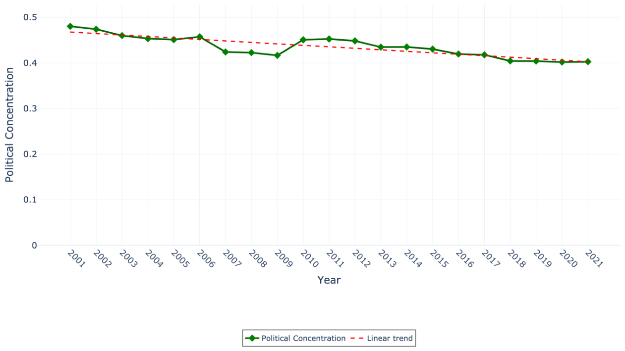
Figure 2.
Spatial Distribution of Political Concentration Across Mexican Municipalities
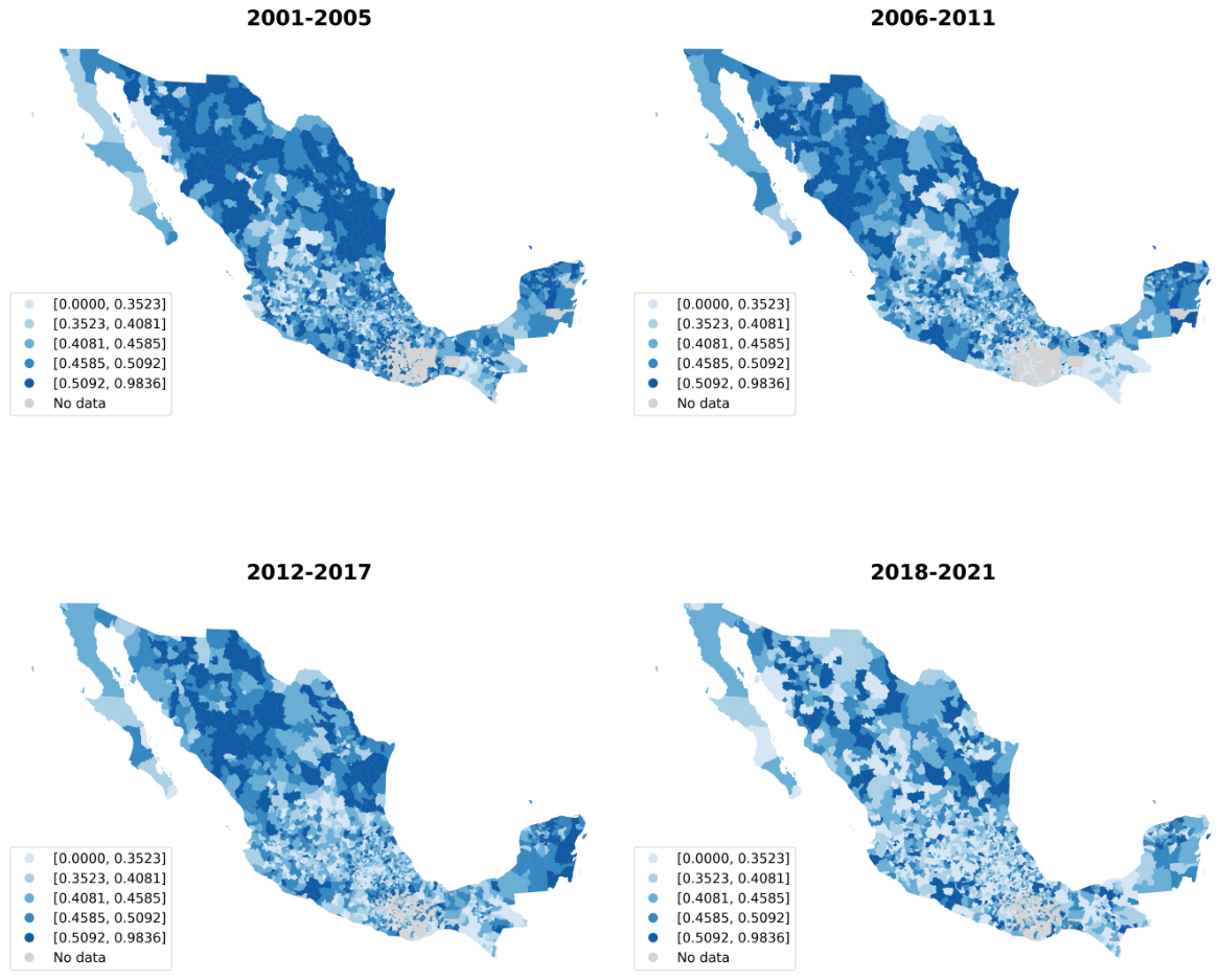
Figure 3.
Structure of Unconditional Transfers to Mexican Municipalities by Government Level
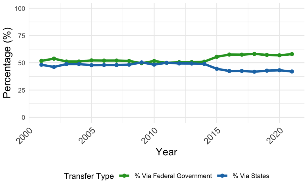
Figure 4.
National and Regional Political Alignment Trends in Mexican Municipalities (2001–2021)
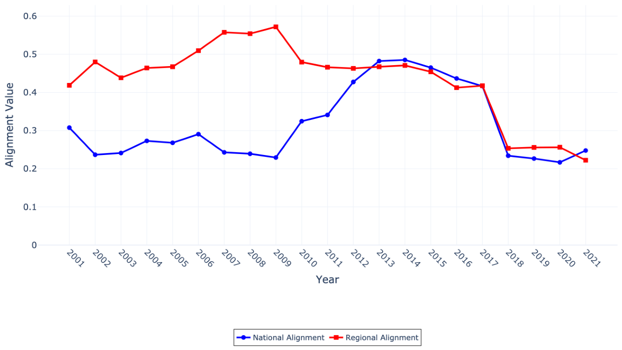
Figure 5.
Spatial Distribution of National Political Alignment Across Mexican Municipalities
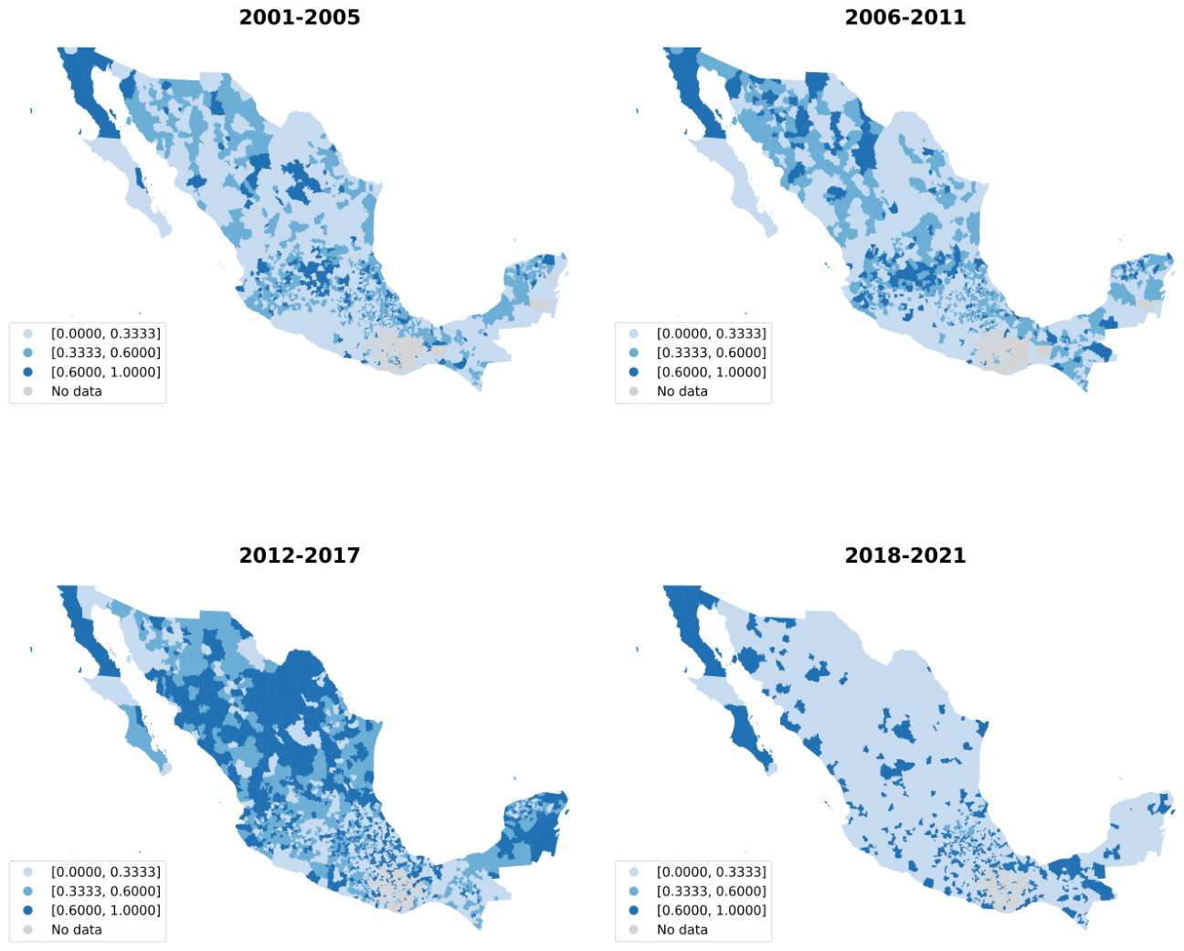
Figure 6.
Spatial Distribution of Regional Political Alignment Across Mexican Municipalities
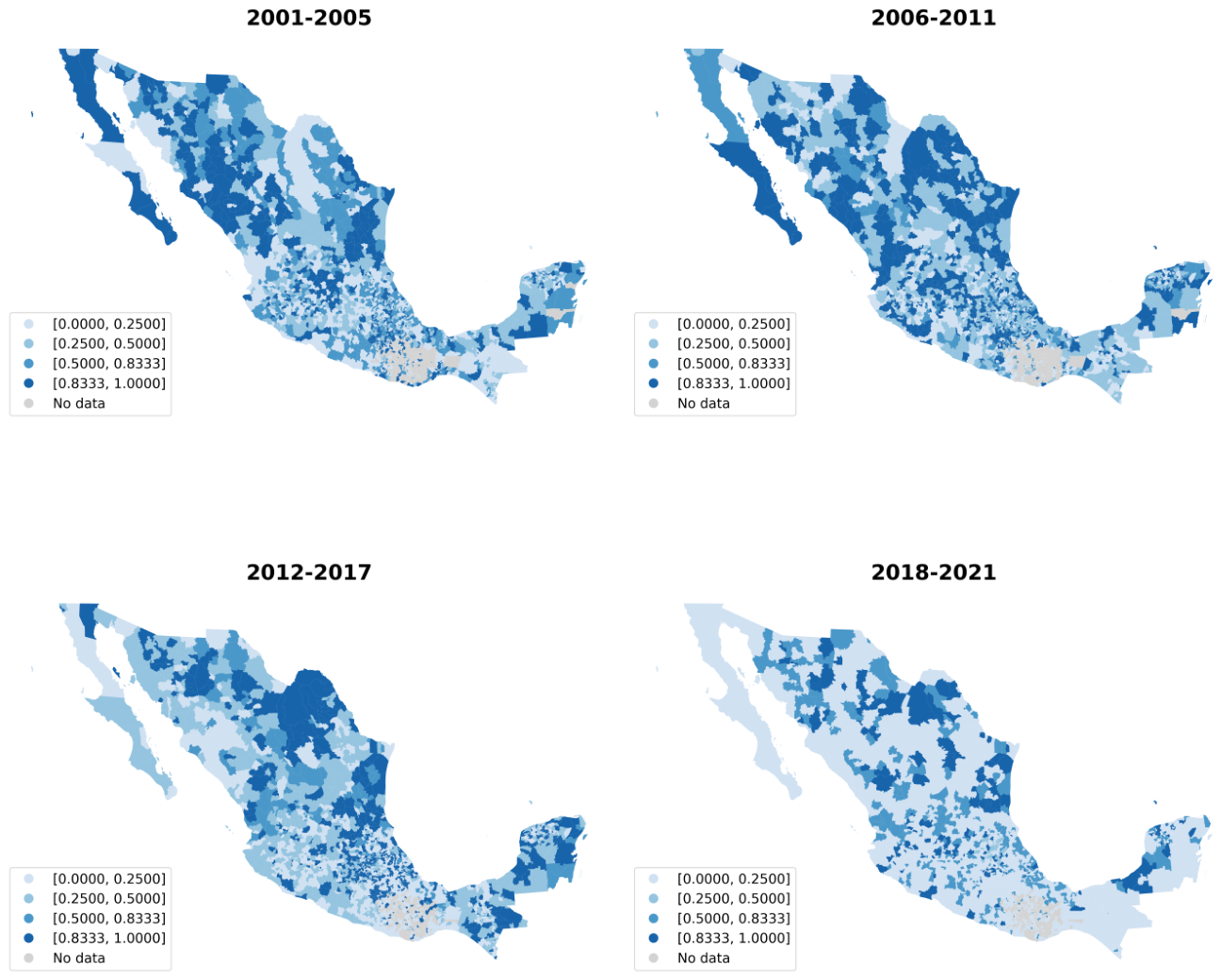
Figure 7.
Temporal Evolution of Political Alignment Categories in Mexican Municipalities
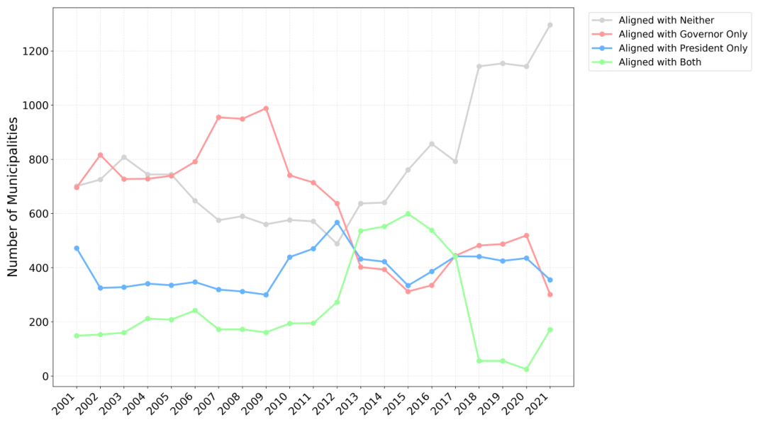
Figure 8.
Predominant Political Alignment Patterns Across Mexican Municipalities (2001–2021)
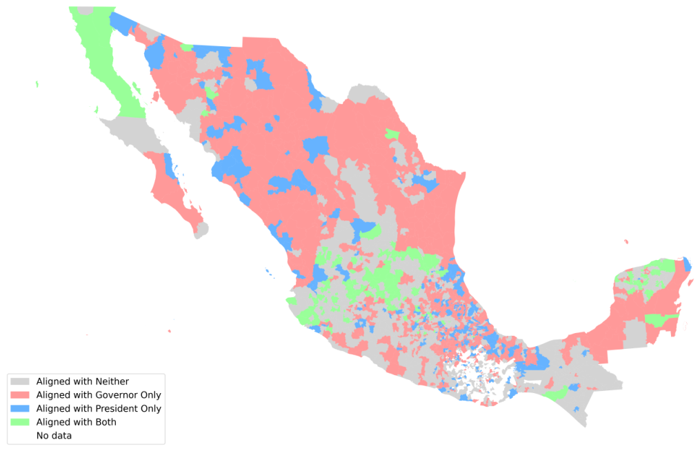
Table 1.
Municipal Political Alignment Patterns (Percentages)
| Period | |||||
|---|---|---|---|---|---|
| Alignment | Overall | 2001– | 2006– | 2012– | 2018– |
| (N) | 2005 | 2011 | 2017 | 2021 | |
| Neither | 37.7 (16,152) | 36.8 | 29.4 | 34.2 | 55.8 |
| Governor Only | 30.7 (13,156) | 36.7 | 42.9 | 20.6 | 21.1 |
| President Only | 19.2 (8,227) | 17.8 | 18.3 | 21.1 | 19.5 |
| Both | 12.3 (5,265) | 8.7 | 9.5 | 24.1 | 3.6 |
Table 2.
Two-Regime Spatial Model Results (Political Concentration, Matrix )
| Political Concentration Threshold | ||||
|---|---|---|---|---|
| Variable | Median (q=50) | q=60 | q=70 | q=80 |
| (Weak Concentration) | 0.23*** | 0.23*** | 0.23*** | 0.23*** |
| [12.66] | [11.06] | [9.56] | [7.25] | |
| (Strong Concentration) | 0.14*** | 0.16*** | 0.17*** | 0.18*** |
| [6.86] | [8.77] | [10.41] | [12.50] | |
| Difference in Spatial Parameters | ||||
| Difference () | 0.09*** | 0.07** | 0.07** | 0.05 |
| t-statistic | [3.04] | [2.35] | [2.12] | [1.28] |
| Covariates | ✓ | ✓ | ✓ | ✓ |
| W*Covariates | ✓ | ✓ | ✓ | ✓ |
| Spatial FE | ✓ | ✓ | ✓ | ✓ |
| Time FE | ✓ | ✓ | ✓ | ✓ |
| Observations | 18,333 | 18,333 | 18,333 | 18,333 |
| R-squared | 0.39 | 0.39 | 0.39 | 0.39 |
| Log-Likelihood | −25,512 | −25,513 | −25,514 | −25,517 |
Note: T-statistics reported in brackets. Significance levels: *** , ** , * . Regimes defined by Equation (14). Finding supports the swing voter hypothesis.
Table 3.
Robustness Check: Consistency of Regime Heterogeneity across Thresholds
| Ranking | Threshold Definition | Predominant Sign | Significant Count | Consistency |
|---|---|---|---|---|
| (Cut-off Percentile) | () | (Total Matrices = 9) | (% Frequency) | |
| 1 | Median () | Positive (+) | 5 | 55.6% |
| 2 | 60th Percentile () | Mixed (predominantly +) | 3 | 33.3% |
| 3 | 70th Percentile () | Mixed (predominantly +) | 3 | 33.3% |
| 4 | 80th Percentile () | Positive (+) | 2 | 22.2% |
Note: Based on estimations using matrices Q1, K1–K5, K10, K15, and Q2. Positive sign supports swing voter hypothesis. At and , the K4 matrix produces significant differences with the opposite sign.
Table 4.
Sensitivity of Political Heterogeneity by Spatial Matrix Specification
| Matrix | Total Significant | Intensity | Dominant Pattern |
|---|---|---|---|
| Specification | Differences | Level | (Key Driver) |
| Q2 | 4 (100%) | Very High | Significant at all thresholds, all positive. |
| K15 (Baseline) | 3 (75%) | High | Significant at Median, 60th, 70th. |
| K4 | 2 (50%) | Medium | Significant at 60th and 70th with negative sign. |
| Q, K3, K5, K10 | 1 (25%) | Low | Single threshold each (Q at 80th, others at Median). |
| K1, K2 | 0 (0%) | Null | No regime heterogeneity detected. |
Note: Total Significant Differences refers to the number of thresholds (out of 4) where was statistically significant.
Table 5.
Two-Regime Spatial Model Results (Vertical Alignment, Matrix )
| Alignment Type | ||
|---|---|---|
| Variable | National Alignment | Regional Alignment |
| (Not Aligned) | 0.135*** | 0.137*** |
| [6.49] | [6.62] | |
| (Aligned) | 0.197*** | 0.199*** |
| [11.38] | [11.17] | |
| Difference in Spatial Parameters | ||
| Difference () | −0.062* | −0.062* |
| t-statistic | [−2.11] | [−2.10] |
| Covariates | ✓ | ✓ |
| W*Covariates | ✓ | ✓ |
| Spatial FE | ✓ | ✓ |
| Time FE | ✓ | ✓ |
| Observations | 17,997 | 17,997 |
| R-squared | 0.388 | 0.388 |
| Log-Likelihood | −25,122.8 | −25,122 |
Note: T-statistics reported in brackets. Significance levels: *** , ** , * . Finding supports the core voter hypothesis.
Table 6.
Robustness Check: Consistency of Alignment Regimes
| Alignment Type | Comparison | Predominant Sign | Significant Count | Consistency |
|---|---|---|---|---|
| (Regime 1 vs 2) | () | (Total Matrices = 9) | (% Frequency) | |
| National (President) | Not Aligned vs Aligned | Negative (−) | 6 | 66.7% |
| Regional (Governor) | Not Aligned vs Aligned | Mixed | 2 | 22.2% |
Note: Negative sign supports core voter hypothesis.
Table 7.
Sensitivity Analysis: Significant Cases by Matrix Intensity
| National Alignment | Regional Alignment | |||
|---|---|---|---|---|
| Matrix Group | Intensity | Significant Cases | Intensity | Significant Cases |
| (Specification) | Level | (Count / Total) | Level | (Count / Total) |
| Global / Dense () | Very High | 1/2 (50%) | Very High | 1/2 (50%) |
| Broad Local () | High | 2/2 (100%) | High | 1/2 (50%) |
| Medium Local () | Medium | 1/1 (100%) | Medium | 0/1 (0%) |
| Sparse Local (–) | Low | 2/4 (50%) | Low | 0/4 (0%) |
| Total Consistency | – | 6/9 (66.7%) | – | 2/9 (22.2%) |
Note: Shows the proportion of matrices in each group where the regime difference was statistically significant ().
Table 8.
Four-Regime Spatial Model Results (National Alignment, )
| Political Concentration Threshold | ||||
|---|---|---|---|---|
| Variable | Median (q=50) | q=60 | q=70 | q=80 |
| (Low Conc, No Nat Align) | 0.144*** | 0.150*** | 0.141*** | 0.107*** |
| [7.83] | [7.57] | [6.50] | [4.46] | |
| (Low Conc, Nat Align) | 0.239*** | 0.183*** | 0.172*** | 0.163*** |
| [8.80] | [6.08] | [5.12] | [4.37] | |
| (High Conc, No Nat Align) | 0.110*** | 0.106*** | 0.133*** | 0.171*** |
| [2.73] | [3.20] | [4.75] | [6.94] | |
| (High Conc, Nat Align) | 0.421*** | 0.445*** | 0.387*** | 0.368*** |
| [8.02] | [11.13] | [11.05] | [11.61] | |
| Differences in Spatial Parameters | ||||
| Regime 1 vs Regime 2 () | −0.095*** | −0.033 | −0.031 | −0.056 |
| [−2.71] | [−0.87] | [−0.74] | [−1.21] | |
| Regime 1 vs Regime 3 () | 0.033 | 0.044 | 0.008 | −0.064* |
| [0.73] | [1.08] | [0.21] | [−1.73] | |
| Regime 1 vs Regime 4 () | −0.277*** | −0.295*** | −0.245*** | −0.261*** |
| [−4.88] | [−6.40] | [−5.76] | [−6.30] | |
| Regime 2 vs Regime 3 () | 0.128** | 0.077* | 0.039 | −0.007 |
| [2.56] | [1.67] | [0.87] | [−0.16] | |
| Regime 2 vs Regime 4 () | −0.182*** | −0.262*** | −0.214*** | −0.204*** |
| [−2.99] | [−5.06] | [−4.26] | [−4.03] | |
| Regime 3 vs Regime 4 () | −0.310*** | −0.339*** | −0.253*** | −0.197*** |
| [−4.64] | [−6.38] | [−5.46] | [−4.71] | |
| Covariates | ✓ | ✓ | ✓ | ✓ |
| W*Covariates | ✓ | ✓ | ✓ | ✓ |
| Spatial FE | ✓ | ✓ | ✓ | ✓ |
| Time FE | ✓ | ✓ | ✓ | ✓ |
| Observations | 17,997 | 17,997 | 17,997 | 17,997 |
| R-squared | 0.387 | 0.388 | 0.387 | 0.387 |
| Log-Likelihood | −25,156.0 | −25,146.6 | −25,152.2 | −25,151.6 |
Note: T-statistics reported in brackets. Significance levels: *** , ** , * . Finding supports core voter hypothesis.
Table 9.
Robustness Check: Frequency and Consistency of National Regime Differences
| Ranking | Comparison | Predominant Sign | Significant Count | Consistency |
|---|---|---|---|---|
| (Pair of Regimes) | (Difference Direction) | (Total = 36) | (% Frequency) | |
| 1 | Regime 1 vs Regime 4 | Negative (−) | 20 | 55.6% |
| 2 | Regime 3 vs Regime 4 | Negative (−) | 14 | 38.9% |
| 3 | Regime 2 vs Regime 4 | Negative (−) | 11 | 30.6% |
| 4 | Regime 2 vs Regime 3 | Mixed (+/−) | 7 | 19.4% |
| 5 | Regime 1 vs Regime 3 | Negative (−) | 7 | 19.4% |
| 6 | Regime 1 vs Regime 2 | Negative (−) | 5 | 13.9% |
Note: Results based on 216 pairwise comparisons. Negative sign indicates , supporting core voter when comparing weaker (A) vs stronger (B) regimes.
Table 10.
Sensitivity of National Heterogeneity by Spatial Matrix Specification
| Matrix | Total Significant | Intensity | Dominant Pattern |
|---|---|---|---|
| Specification | Differences | Level | (Key Driver) |
| Q2 | 15 | Very High | Strong distinction of Regimes 3 & 4 vs others. |
| K15 | 14 | Very High | Regime 4 is significantly higher than R1/R2/R3. |
| K10 | 11 | High | Consistent differences driven by Regime 4. |
| K5 | 10 | Medium | Regime 4 consistently distinct. |
| K2 | 5 | Low | Scattered differences (mostly 1 vs 4). |
| K3 | 4 | Low | Weak detection of heterogeneity. |
| Q1 | 3 | Low | Only significant at extreme percentiles. |
| K4 | 2 | Very Low | Anomalous positive difference (1 vs 3). |
| K1 | 0 | Null | No regime heterogeneity detected. |
Table 11.
Four-Regime Spatial Model Results (Regional Alignment, )
| Political Concentration Threshold | ||||
|---|---|---|---|---|
| Variable | Median (q=50) | q=60 | q=70 | q=80 |
| (Low Conc, No Reg Align) | 0.167*** | 0.131*** | 0.123*** | 0.102*** |
| [8.50] | [6.24] | [5.41] | [4.05] | |
| (Low Conc, Reg Align) | 0.181*** | 0.203*** | 0.197*** | 0.160*** |
| [7.49] | [7.62] | [6.52] | [4.69] | |
| (High Conc, No Reg Align) | 0.433*** | 0.457*** | 0.376*** | 0.356*** |
| [9.04] | [11.99] | [11.78] | [12.76] | |
| (High Conc, Reg Align) | 0.080* | 0.069* | 0.107*** | 0.143*** |
| [1.82] | [1.95] | [3.51] | [5.19] | |
| Differences in Spatial Parameters | ||||
| Regime 1 vs Regime 2 () | −0.014 | −0.072** | −0.074 | −0.058 |
| [−0.41] | [−1.99] | [−1.86] | [−1.31] | |
| Regime 1 vs Regime 3 () | −0.266*** | −0.326*** | −0.253*** | −0.255*** |
| [−4.97] | [−7.17] | [−6.15] | [−6.41] | |
| Regime 1 vs Regime 4 () | 0.088 | 0.062 | 0.016 | −0.041 |
| [1.78] | [1.47] | [0.40] | [−1.06] | |
| Regime 2 vs Regime 3 () | −0.252*** | −0.255*** | −0.179*** | −0.197*** |
| [−4.59] | [−5.31] | [−3.95] | [−4.35] | |
| Regime 2 vs Regime 4 () | 0.101 | 0.134*** | 0.090** | 0.017 |
| [1.95] | [2.89] | [1.98] | [0.37] | |
| Regime 3 vs Regime 4 () | 0.353*** | 0.388*** | 0.269*** | 0.214*** |
| [5.37] | [7.25] | [5.84] | [5.19] | |
| Covariates | ✓ | ✓ | ✓ | ✓ |
| W*Covariates | ✓ | ✓ | ✓ | ✓ |
| Spatial FE | ✓ | ✓ | ✓ | ✓ |
| Time FE | ✓ | ✓ | ✓ | ✓ |
| Observations | 17,997 | 17,997 | 17,997 | 17,997 |
| R-squared | 0.387 | 0.388 | 0.387 | 0.387 |
| Log-Likelihood | −25,155.5 | −25,137.6 | −25,148.6 | −25,148.9 |
Note: T-statistics reported in brackets. Significance levels: *** , ** , * . Finding indicates that high concentration without regional alignment exhibits stronger mimicking than high concentration with regional alignment.
Table 12.
Robustness Check: Frequency and Consistency of Regional Regime Differences
| Ranking | Comparison | Predominant Sign | Significant Count | Consistency |
|---|---|---|---|---|
| (Pair of Regimes) | (Difference Direction) | (Total = 36) | (% Frequency) | |
| 1 | Regime 1 vs Regime 3 | Negative (−) | 22 | 61.1% |
| 2 | Regime 2 vs Regime 3 | Negative (−) | 21 | 58.3% |
| 3 | Regime 3 vs Regime 4 | Positive (+) | 21 | 58.3% |
| 4 | Regime 2 vs Regime 4 | Mixed | 6 | 16.7% |
| 5 | Regime 1 vs Regime 4 | Mixed | 5 | 13.9% |
| 6 | Regime 1 vs Regime 2 | Negative (−) | 3 | 8.3% |
Note: Results based on 216 pairwise comparisons. Positive sign for 3 vs 4 indicates : high concentration without regional alignment mimics more than with alignment.
Table 13.
Sensitivity of Regional Heterogeneity by Spatial Matrix Specification
| Matrix | Total Significant | Intensity | Dominant Pattern |
|---|---|---|---|
| Specification | Differences | Level | (Key Driver) |
| K15 | 15 | Very High | Regime 3 is the structural outlier (Highest ). |
| Q2 | 15 | Very High | Consistent hierarchy with R3 at top. |
| K10 | 14 | Very High | Strong positive difference for 3 vs 4. |
| K5 | 10 | Medium | Consistent detection of R3 heterogeneity. |
| Q1 | 9 | High | Significant differences in R3 vs R4. |
| K1, K2 | <5 | Low | Weak detection in sparse matrices. |
Table 17.
Difference-in-Differences Results (PCI × Vertical Alignment, )
| National Alignment | Regional Alignment | |||||||
|---|---|---|---|---|---|---|---|---|
| Median | q=60 | q=70 | q=80 | Median | q=60 | q=70 | q=80 | |
| 0.215** | 0.305*** | 0.222*** | 0.141* | −0.272*** | −0.343*** | −0.460*** | −0.367*** | |
| t-statistic | [2.92] | [4.83] | [3.70] | [2.35] | [−4.71] | [−5.89] | [−7.41] | [−5.10] |
| Interpretation | PCI effect stronger among non-aligned | PCI effect stronger among aligned | ||||||
Note: T-statistics in brackets. Significance levels: *** , ** , * . as defined in Equation (22).
Table 18.
Robustness Check: Consistency of DiD across Matrix Specifications
| National Alignment | Regional Alignment | |||||
|---|---|---|---|---|---|---|
| Threshold | Sign | Sig. Count | Consistency | Sign | Sig. Count | Consistency |
| 80th | (+) | 4/9 | 44.4% | (−) | 6/9 | 66.7% |
| 70th | (+) | 2/9 | 22.2% | (−) | 6/9 | 66.7% |
| 60th | (+) | 2/9 | 22.2% | (−) | 5/9 | 55.6% |
| Median | (+) | 2/9 | 22.2% | (−) | 2/9 | 22.2% |
Note: Based on estimations using matrices Q1, K1–K5, K10, K15, and Q2.
Table 19.
Summary of Evidence for Swing Voter versus Core Voter Hypotheses
| Specification | Key Finding | Swing Voter | Core Voter | Interpretation |
|---|---|---|---|---|
| PCI (2 regimes) | ✓ | Weak mimics more | ||
| NA (2 regimes) | ✓ | Aligned mimics more | ||
| RA (2 regimes) | ✓ | Aligned mimics more | ||
| PCI × NA (4 regimes) | ✓ | Strongest mimics most | ||
| PCI × RA (4 regimes) | RA reverses PCI effect | |||
| NA × RA (4 regimes) | ✓ | Isolated mimics most |
Disclaimer/Publisher’s Note: The statements, opinions and data contained in all publications are solely those of the individual author(s) and contributor(s) and not of MDPI and/or the editor(s). MDPI and/or the editor(s) disclaim responsibility for any injury to people or property resulting from any ideas, methods, instructions or products referred to in the content. |
© 2026 by the authors. Licensee MDPI, Basel, Switzerland. This article is an open access article distributed under the terms and conditions of the Creative Commons Attribution (CC BY) license (http://creativecommons.org/licenses/by/4.0/).
Copyright: This open access article is published under a Creative Commons CC BY 4.0 license, which permit the free download, distribution, and reuse, provided that the author and preprint are cited in any reuse.