
Submitted:
19 October 2026
Posted:
20 October 2026
You are already at the latest version
Abstract
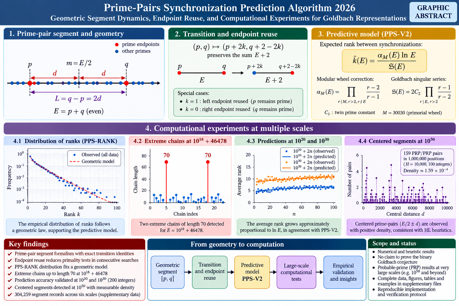
We introduce a prime-pair segment formalism for the binary Goldbach problem and an algorithmic framework for propagating verified or probable-prime decompositions between consecutive even integers. A segment [p,q] is associated with an even target E=p+q, center m=E/2, half-length d=m−p, and full length L=q−p=2d. A general transition (p,q)↦(p+2k,q+2−2k) preserves the sum E+2, with d↦d+1−2k. The special cases k=1 and k=0 preserve one endpoint and permit computational reuse of an existing primality result when the other endpoint is prime. We describe an auditable implementation with exact enumeration for moderate integers, window-limited searches for larger integers, and explicitly conditional probable-prime results near 10^2000.A supplementary dataset contains 304,259 recorded segment rows for 98 sampled even integers across six base scales. We emphasize that endpoint propagation is an exact identity but not an unconditional primality predictor. We cite twelve separately supplied figures and twelve tables, computational controls, failure modes, and a reproducibility agenda. No claim is made to prove the binary Goldbach conjecture or to exhaustively enumerate representations for enormous targets.
Keywords:
Goldbach conjecture
; prime pairs
; synchronization
; integer segments
; computational number theory
; primality testing
; predictive search
; prime gaps
1. Introduction
The binary Goldbach conjecture asserts that every even integer greater than two is a sum of two primes. The classical Hardy–Littlewood framework anticipates the density of representations while distinguishing asymptotic heuristics from proofs [1]. Vinogradov’s work on three primes and Helfgott’s subsequent unconditional ternary theorem establish a related but distinct result [2,4,5,6]. Chen’s theorem supplies a prime plus an almost-prime for sufficiently large even targets, but does not remove the parity obstacle for binary Goldbach [3].
Extensive computational verification provides valuable finite evidence, notably the work of Oliveira e Silva, Herzog and Pardi [7], while Helfgott and Platt illustrate rigorous numerical certification in the ternary setting [8]. Related contributions on additive prime decompositions and exceptional sets underscore the need to separate analytical theorems from numerical experimentation [9,10,11]. Our approach is deliberately narrower: it asks whether the geometry of a known decomposition can organize subsequent searches and avoid redundant primality tests.
The proposed method is not a substitute for the circle method, whose analytic background is surveyed in standard accounts [12,13]. Instead, it defines a data structure, transition map and evaluation protocol for a specific computational objective: identifying prime endpoints efficiently and reporting precisely what has and has not been proved.
2. Mathematical Definition of a Prime-Pair Segment
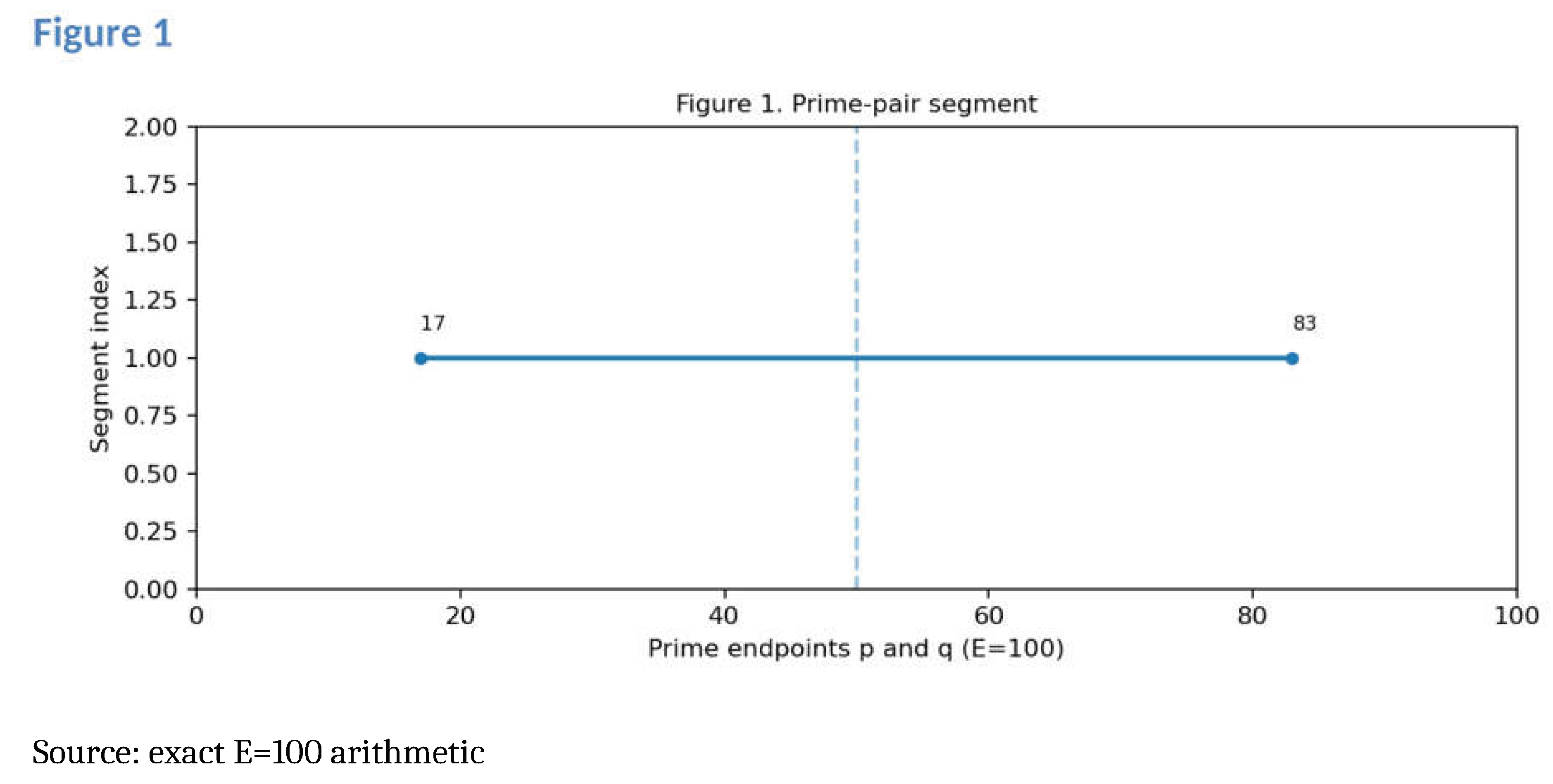
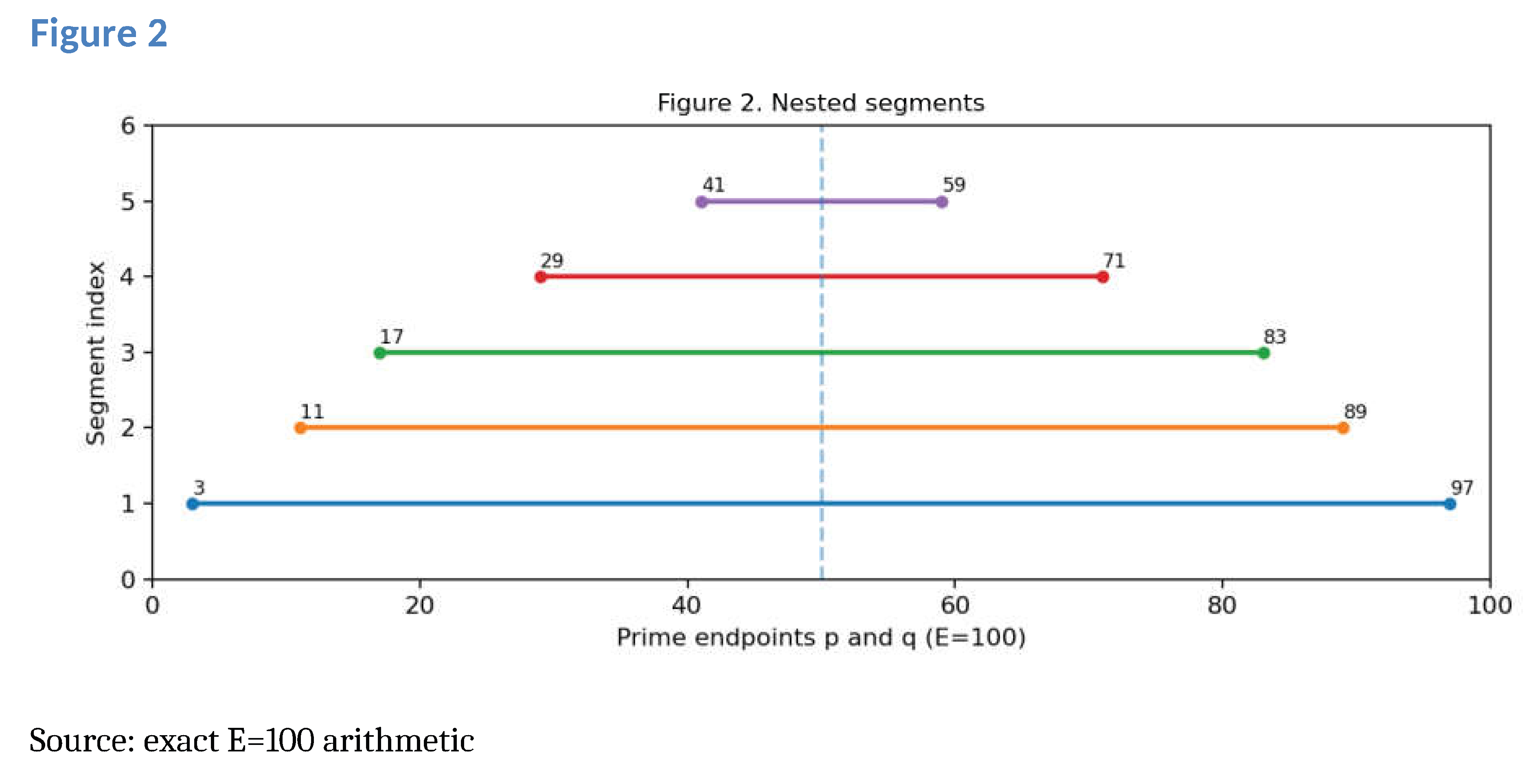
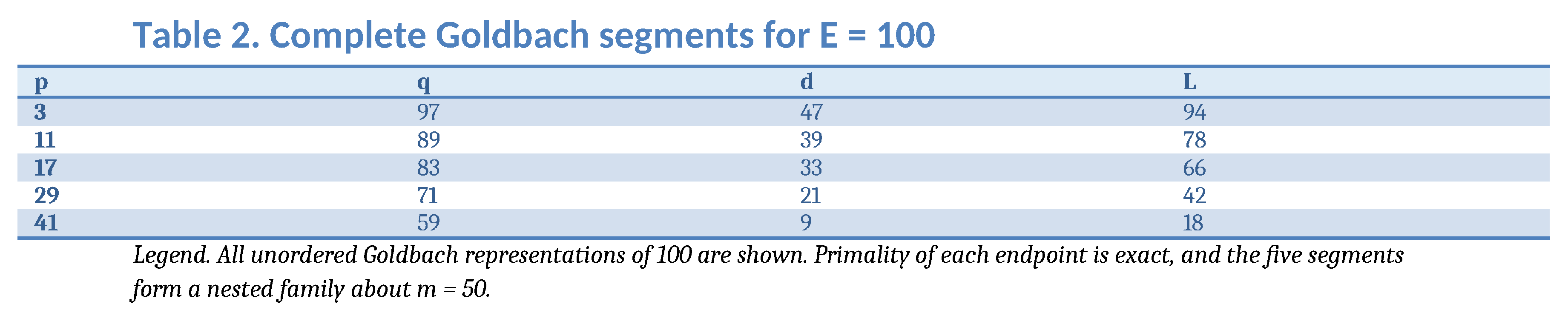
Figure 1 defines a prime-pair segment and its midpoint, while Figure 2 illustrates nested symmetric segments for a fixed even integer. Figure 7 explains the central distance and segment length, and Figure 8 schematically illustrates the distribution of segments around a common midpoint. Table 1 summarizes the mathematical definitions; Table 2 provides the five exact decompositions of E = 100. These displays distinguish a geometric interval from the separate requirement that both endpoints be prime.
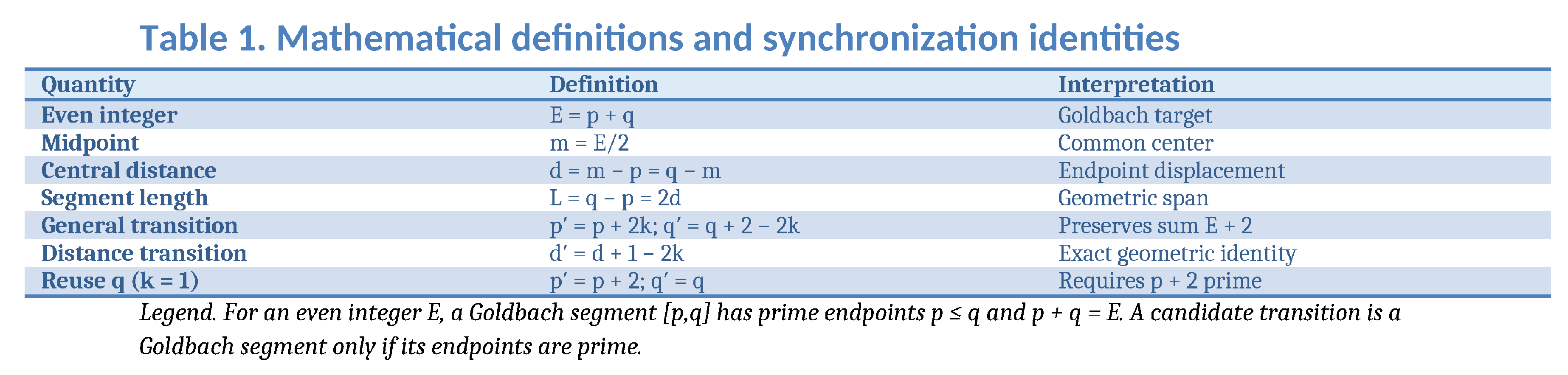
The segment convention used here is [p,q] with p ≤ q and p + q = E. The Euclidean length q − p is not E; rather, it equals 2d. This distinction matters for reproducibility, because the integer E labels the representation and its midpoint, whereas L = q − p measures the span of its endpoints.
Let E≥4 be even and let p≤q be primes with p+q=E. Define the Goldbach prime-pair segment [p,q] as the closed integer interval with prime endpoints p and q, associated with the sum constraint. The midpoint is m=E/2, the central displacement is d=m−p=q−m, and the length is L=q−p=2d. This is an interval, not an assertion that all its interior integers are prime. The designation “segment” refers only to its two prime endpoints and their geometric relationship.
For fixed E, all admissible segments share the same midpoint; their lengths encode their positions in the representation spectrum. The smallest p corresponds to the largest d, whereas a centrally close pair has a small d. The degenerate case p=q can occur when E=2p; then d=L=0. For even E>4 and odd-prime endpoints, p and q are odd and d is integral, but the parity of d depends on the parity of m.
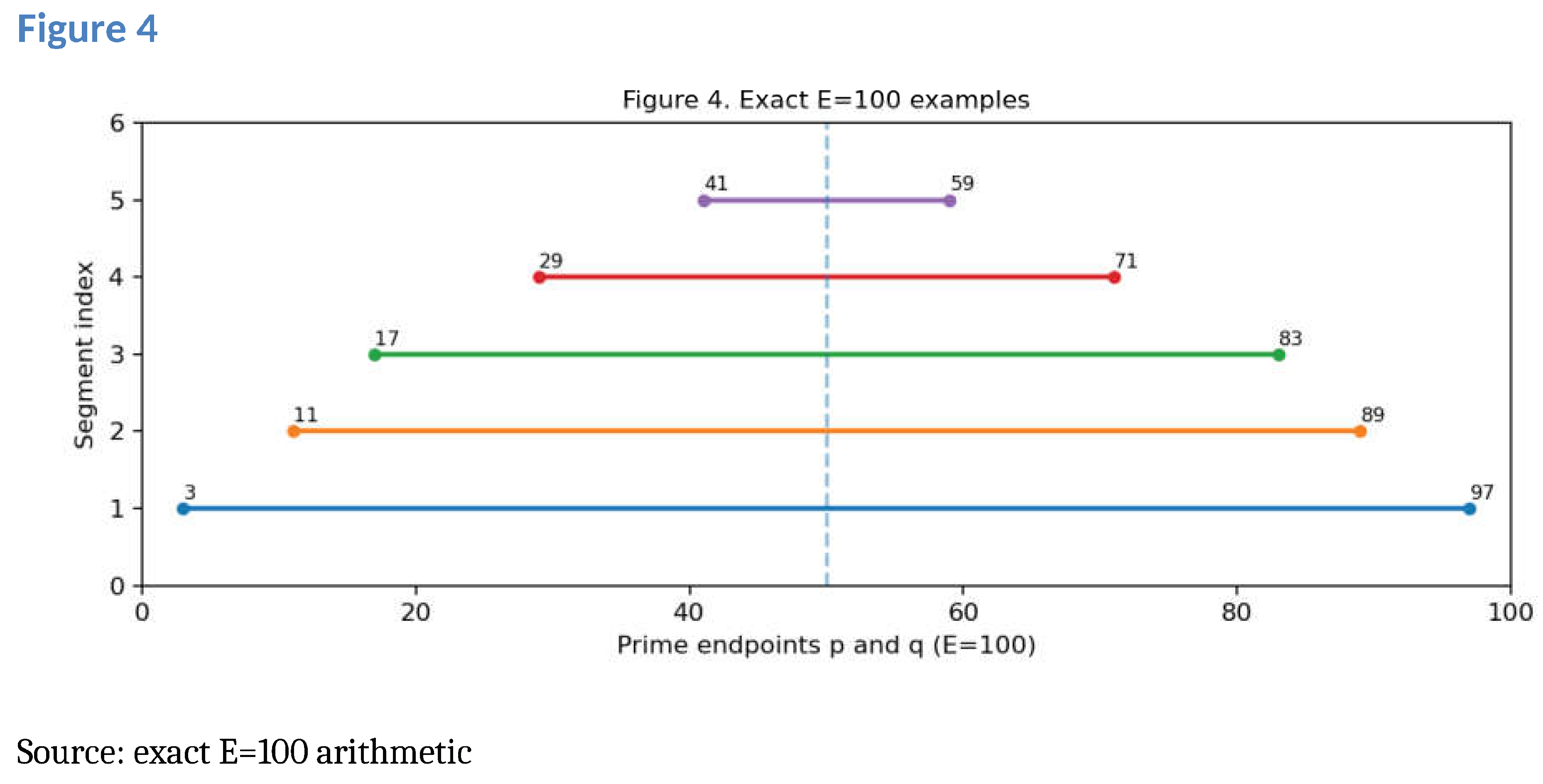
For E=100, the exact decompositions are (3,97), (11,89), (17,83), (29,71) and (41,59). These five examples provide an entirely auditable model for Figures 1 and 2 and Table 2. All five endpoints can be verified by trial division.
3. Exact Synchronization and the Prediction Map
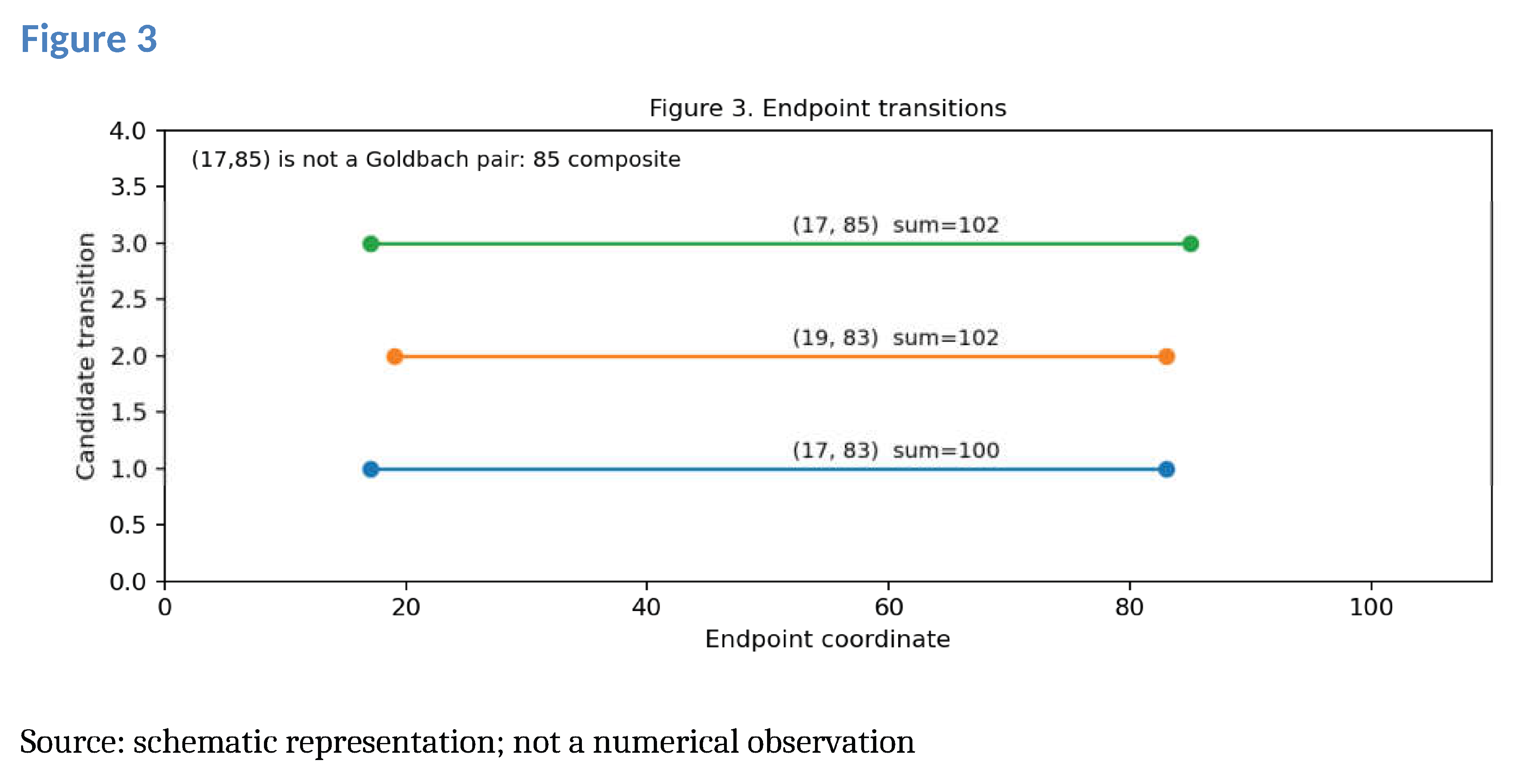
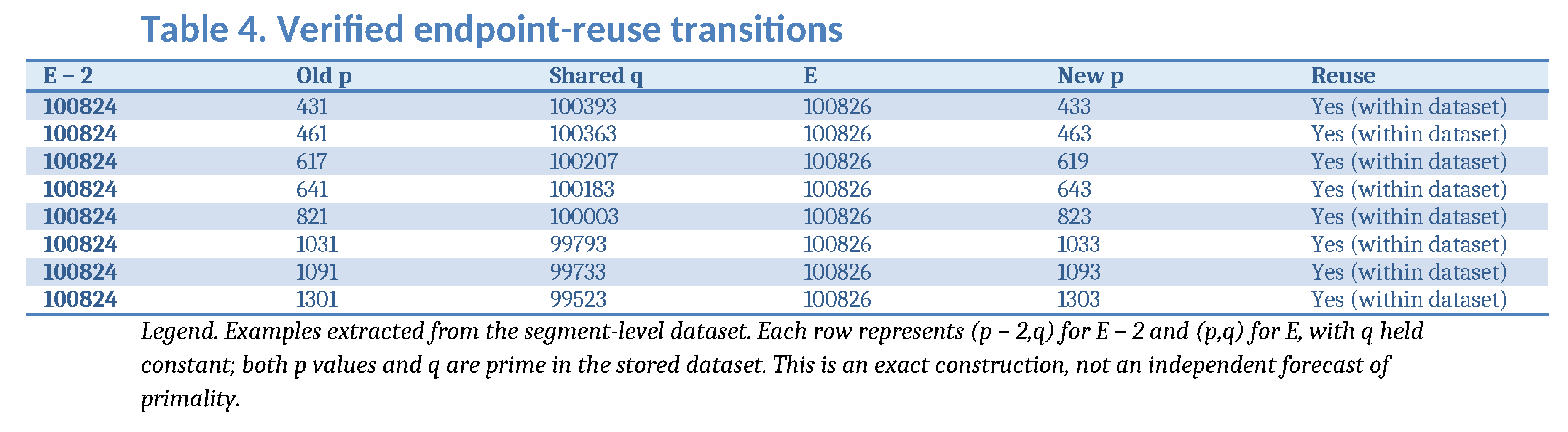
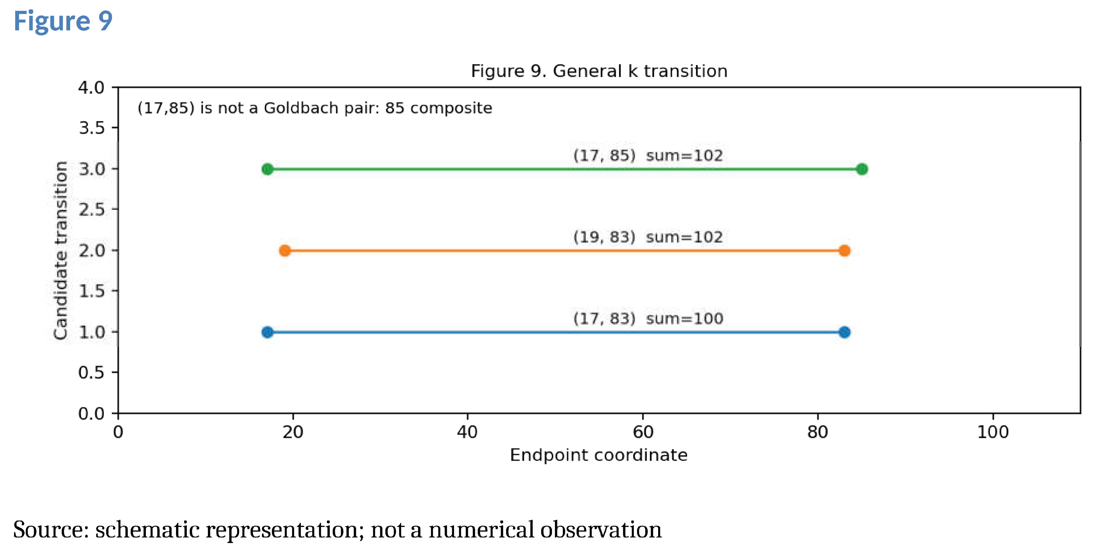
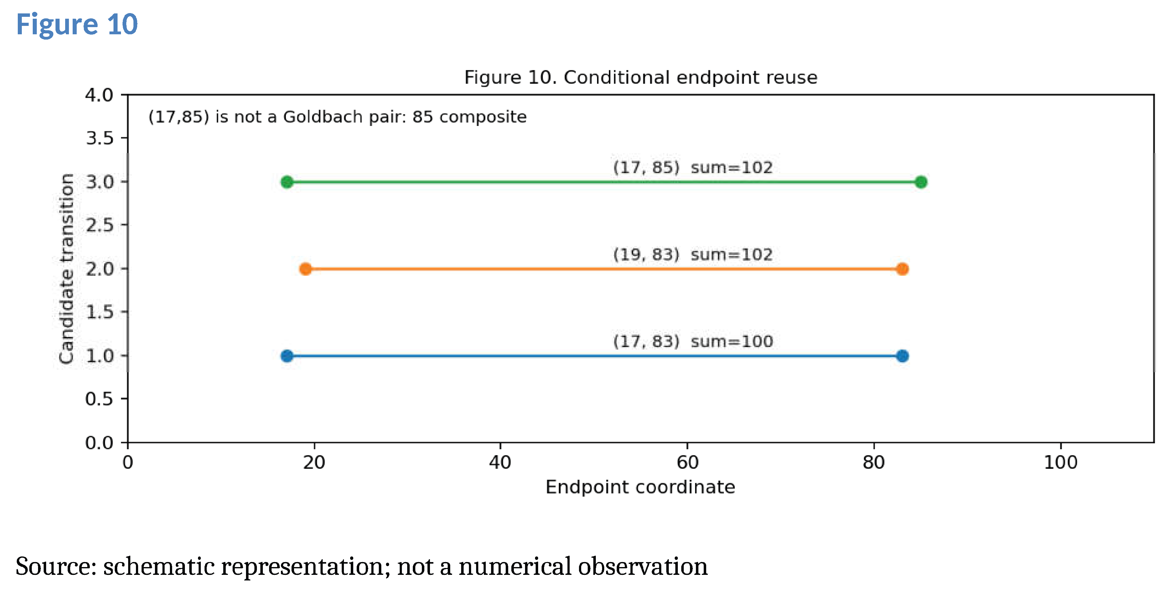
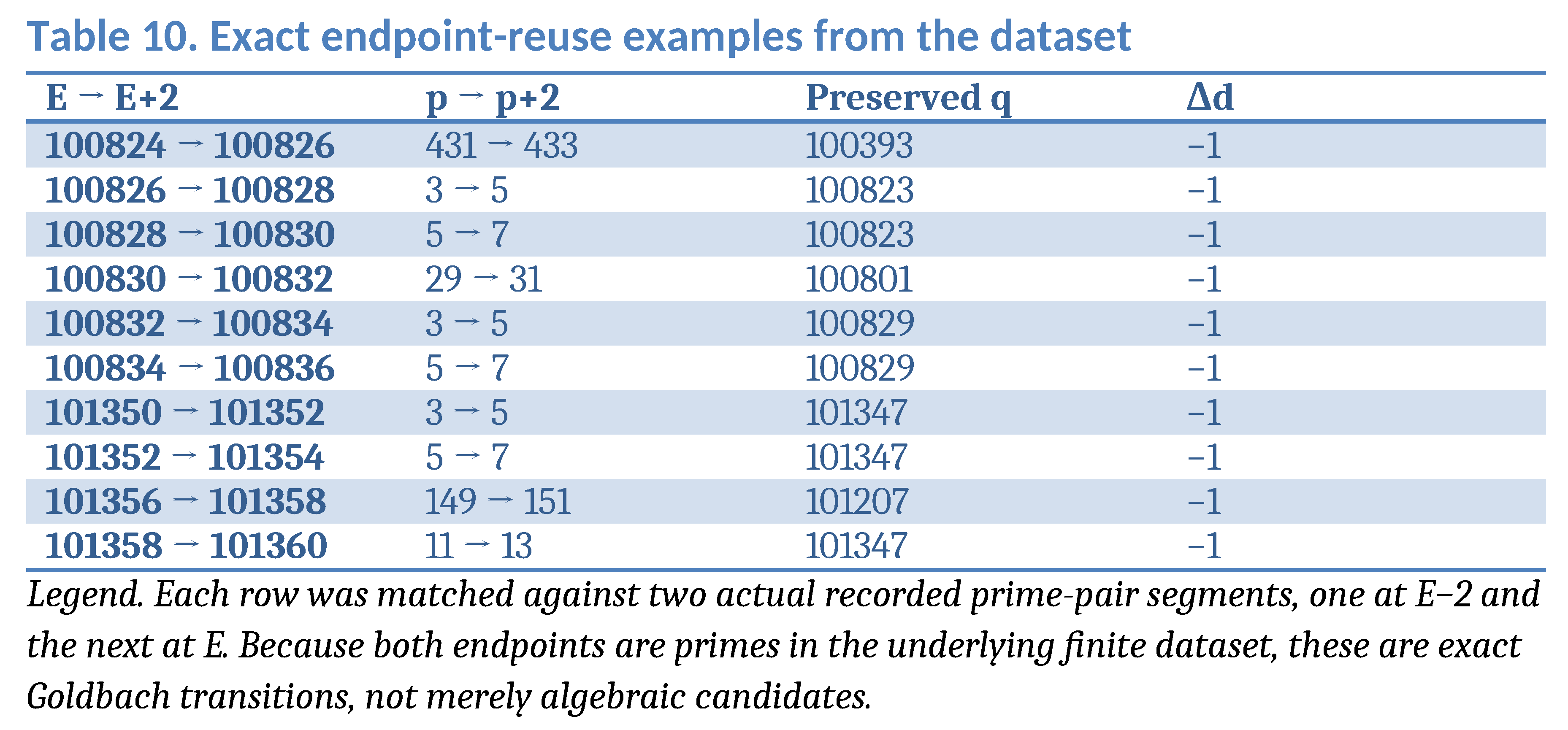
Figure 3 illustrates both endpoint-preserving transitions from E to E+2. Figure 9 gives the general k-parameter transformation and its two elementary cases. Figure 10 depicts conditional propagation across successive even integers. Table 4 records verified finite endpoint-reuse transitions, while Table 10 lists further exact examples. None of these diagrams establishes primality of an untested endpoint. Table 11 contrasts exploratory large-number candidates and the corresponding limits of primality certification.
The identities are unconditional algebraic statements. The additional assertion that (p′,q′) is a Goldbach pair is conditional on both endpoints being prime. For a probable-prime anchor, reuse propagates only the previous probable-prime status; it does not upgrade the evidence to a proof.
Suppose E=p+q with both endpoints prime. For an integer k, define p′=p+2k and q′=q+2−2k. Direct addition yields p′+q′=E+2. Because m′=m+1, the central displacement becomes d′=m′−p′=d+1−2k. These equalities are algebraic identities for any integer k, whether or not the new endpoints are prime.
For k=1, q′=q and p′=p+2. A valid representation of E+2 follows exactly when p+2 is prime. For k=0, p′=p and q′=q+2; this is valid exactly when q+2 is prime. In both cases one endpoint is reused, so an existing certificate or accepted probable-prime result for that endpoint can be reused without recomputation. In contrast, the identity itself cannot certify the changed endpoint.
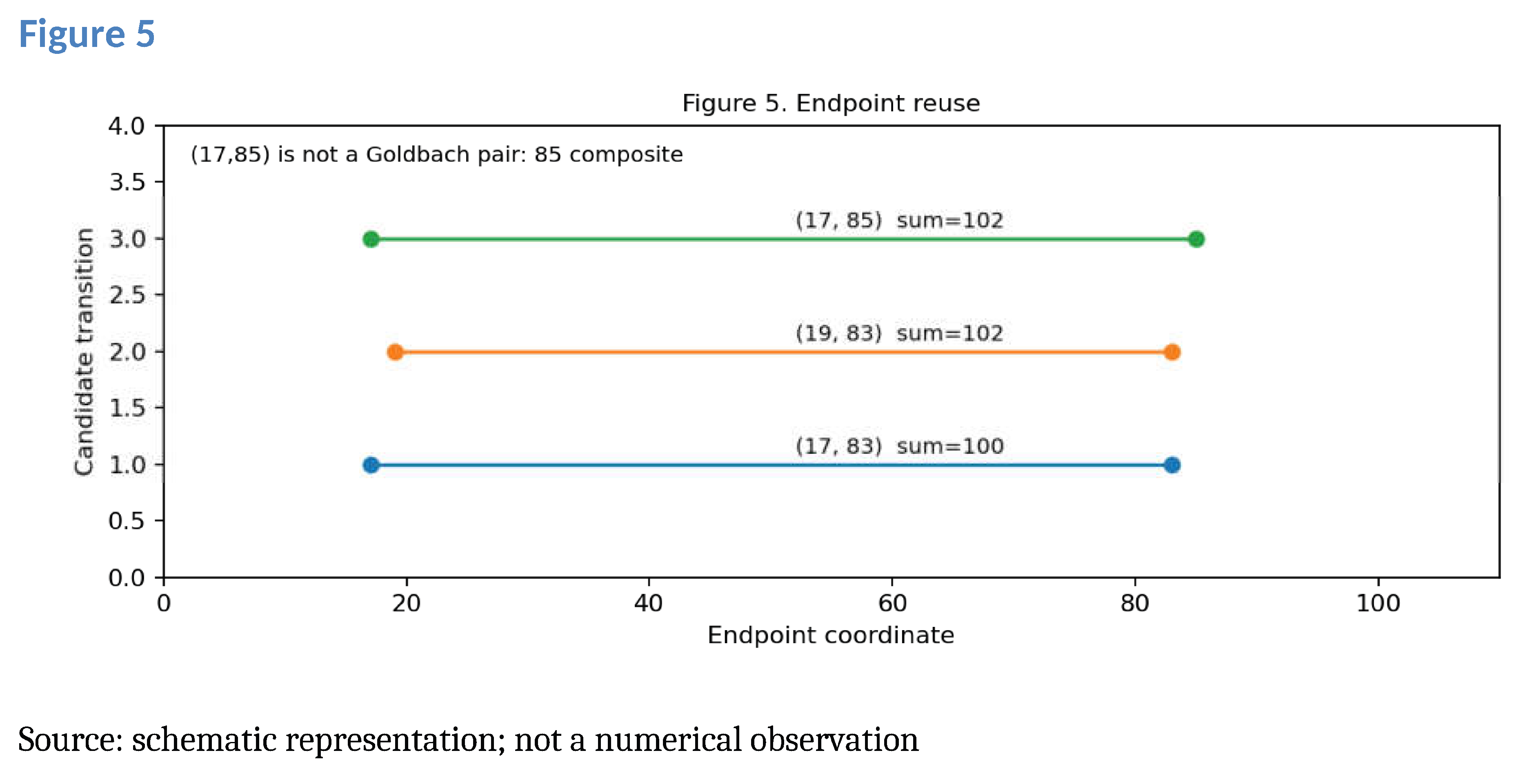
For example, 100=17+83 and 102=19+83. The first endpoint increases by two while the second remains the same. This exact finite example shows the mechanism without reliance on a heuristic model. Figure 3 illustrates the two elementary d-updates. Figure 4 instead depicts the complete prime-pair structure of E=100, an independent finite control.
4. Relationship to Prime Tuples and Prime Gaps
The k=1 continuation requires both p and p+2 to be prime; hence it is a twin-prime condition on the moving endpoint. The k=0 continuation requires q and q+2 to be prime. Consequently, the method is related to prime-pair and prime-tuple phenomena rather than to a new implication of Goldbach itself. Work on small and bounded gaps by Goldston, Pintz and Yıldırım [17], Zhang [18], Maynard [19] and Polymath [20] provides relevant theoretical context but does not guarantee an endpoint-preserving continuation for every even E.
Prime-gap models and short-interval heuristics, including those of Gallagher [21], Cramér [22] and Granville [23], motivate statistical baseline comparisons. They should not be used as proofs that a proposed segment is prime. Estimates for the distribution of primes [24,25] help frame search-window selection, whereas sieve methods [14,15,16,26] explain how modular filters can eliminate many composite candidates cheaply.
A particularly important failure mode is the following: the existence of a Goldbach representation for E does not imply that either endpoint can be increased by two while remaining prime. The transition mechanism may fail even when E+2 has many unrelated Goldbach representations. We therefore distinguish endpoint persistence, fresh-anchor discovery and full enumeration.
5. Algorithm and Computational Protocol
5.1. Candidate Generation
For each selected even target E, enumerate candidate primes p≤min(E/2,H), where H is a declared search bound. Set q=E−p. Apply inexpensive modular filters to q before a strong primality test. For each successful candidate, record E,p,q,m,d,L, the bound H, the primality status of each endpoint, and the computational evidence. If H=E/2 and every eligible p is considered, the result is exhaustive; otherwise it is a window-limited list.
When E is very large, H may be a few thousand or hundred thousand, making the search feasible without implying anything about the remaining vast interval. A prime p can be tested exactly by deterministic methods at small sizes; a positive probable-prime test for a 2000-digit q must be labeled PRP unless a primality proof is supplied.
5.2. Prediction-First Transition
Given the list of representations at E, construct the k=1 proposals (p+2,q) and optionally k=0 proposals (p,q+2). Check only the moving endpoint. Deduplicate identical proposals and record whether a result was obtained by reuse or by a fresh search. A fair efficiency benchmark must compare total wall-clock time, modular operations and strong primality calls against a conventional search using the same sieve, search bound and success criterion.
Probabilistic primality methods originate in foundational work by Miller [27] and Rabin [28]; Lucas-based probable-prime tests are discussed by Baillie and Wagstaff [29]. For applications demanding rigorous proof, polynomial-time primality theory provides an important distinction between decision procedures and practical certificates [30].
5.3. Explicit Pseudocode
INPUT: even E, bound H, known representations R(E−2). STEP 1: for each (p,q) in R(E−2), test p+2 and, if prime, emit (p+2,q). STEP 2: optionally test q+2 and, if prime, emit (p,q+2). STEP 3: if more coverage is needed, sieve and test p≤H with q=E−p. STEP 4: verify p+q=E and the status of both endpoints. STEP 5: write a record with provenance and a label of EXACT, CERTIFIED, PRP or REJECTED. OUTPUT: deduplicated records, work counters and search-coverage statement.
6. Experimental Data and Sampling Design
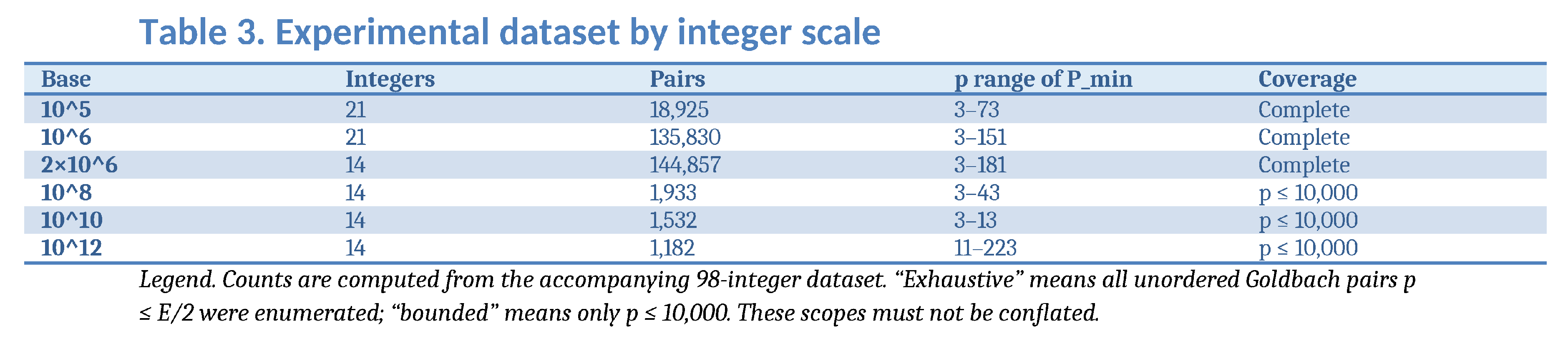
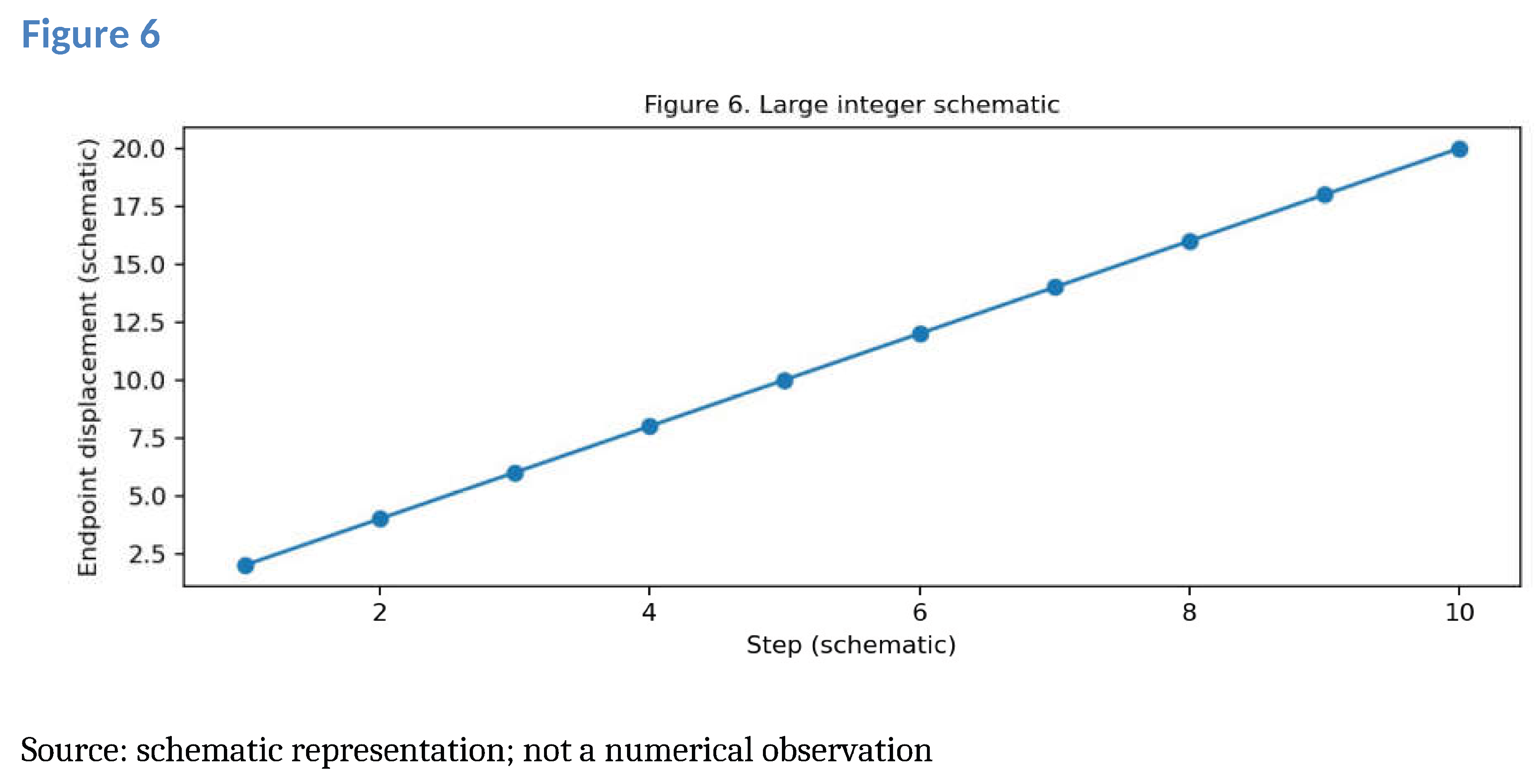
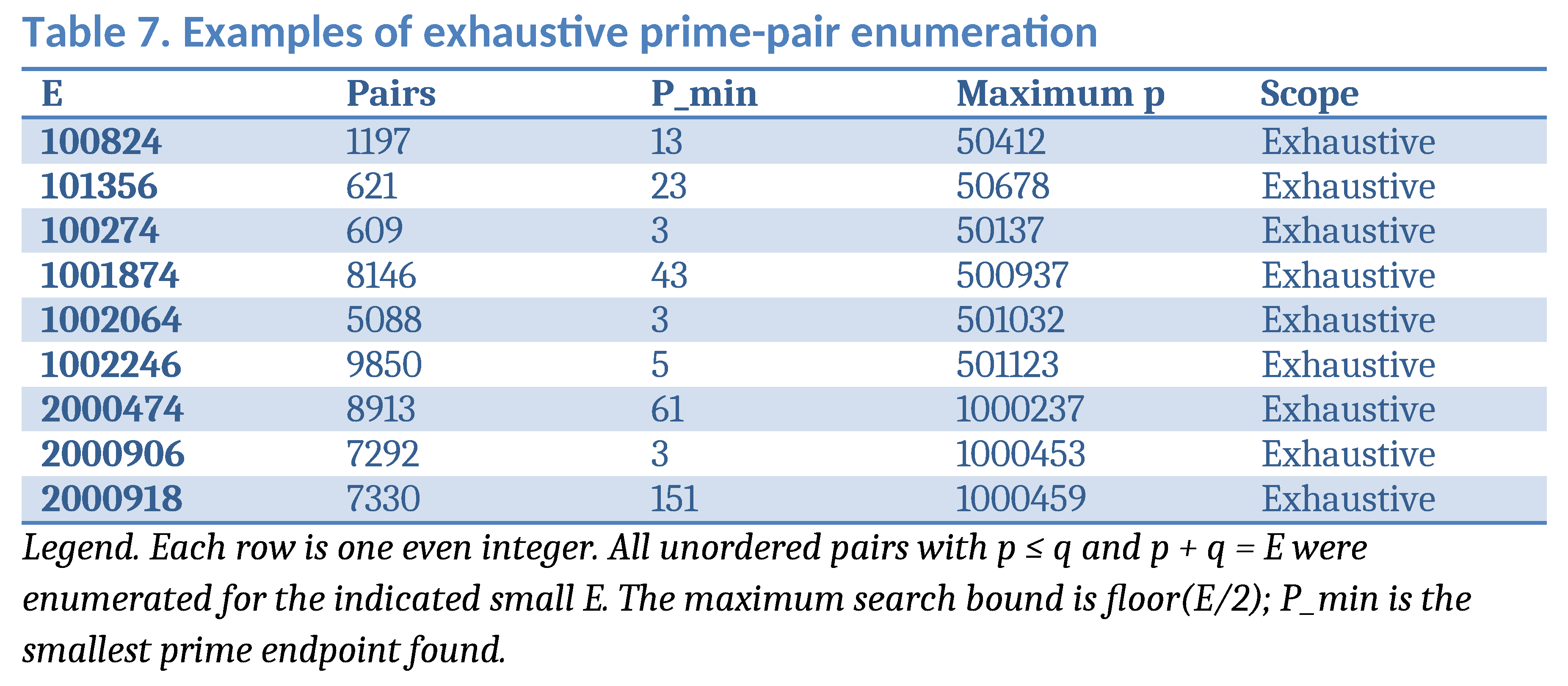
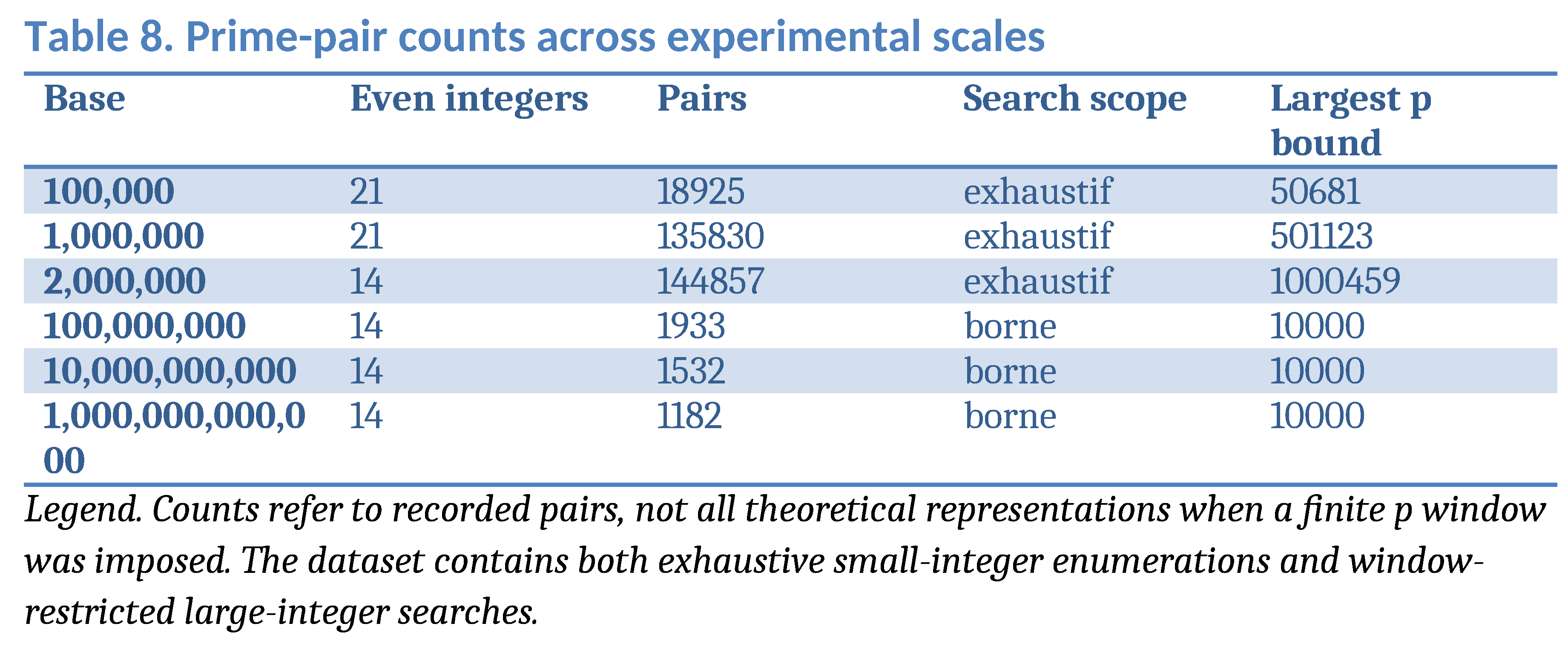
Table 3 summarizes the experimental dataset by integer scale, and Table 8 compares recorded prime-pair counts across scales. Table 7 identifies examples designated as exhaustive, subject to independent audit. Figure 5 illustrates a schematic E-to-E+2 transition, whereas Figure 6 depicts a symbolic large-integer segment; neither is a count-by-scale chart. Numerical comparisons are descriptive because search windows differ.
An apparent decline in the number of segments at larger E can result from restricting the smaller endpoint p rather than from a decline in Goldbach representations. All reported rates therefore require a denominator describing the candidate range and the sampling rule.
The accompanying Supplementary File S1 contains 304,259 recorded segment rows for 98 sampled even targets across six base scales. The target families were constructed as E=B+c+2n using reproducible offsets. The three smaller base scales were marked exhaustive in the source file; the three larger scales were bounded to p≤10^4. In the absence of a fully independent re-execution of every record in this manuscript preparation, the dataset is presented as a computational record whose finite arithmetic, primality, coverage and reuse fields were independently rechecked as detailed in the final audit statement; this remains a finite computational result, not a universal theorem.
The total is not a count of independent even integers: several hundred thousand segment rows arise from only 98 sampled targets. The data are also not a random sample of all even integers, and the endpoint-reuse rate is conditional on the chosen search window. The selection protocol must therefore be fixed before using the data to claim predictive performance.
7. Verified Elementary Examples and Segment Geometry
Figure 4 illustrates the five exact segments for E=100; Figure 7 defines their central distances and lengths, and Figure 8 gives a schematic nested-segment representation for fixed E. Table 2 provides an independently checkable benchmark, while Table 7 describes the coverage of selected enumerations. Schematic arcs must not be interpreted as empirical density estimates.
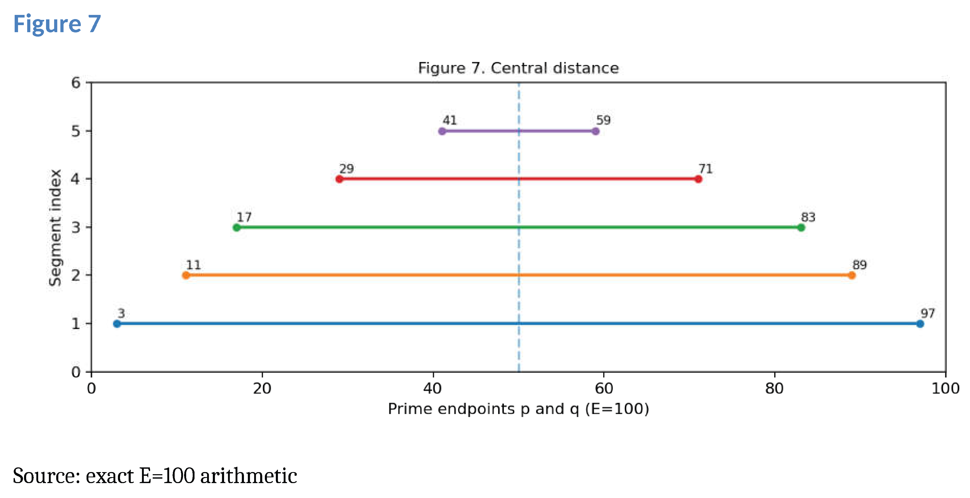
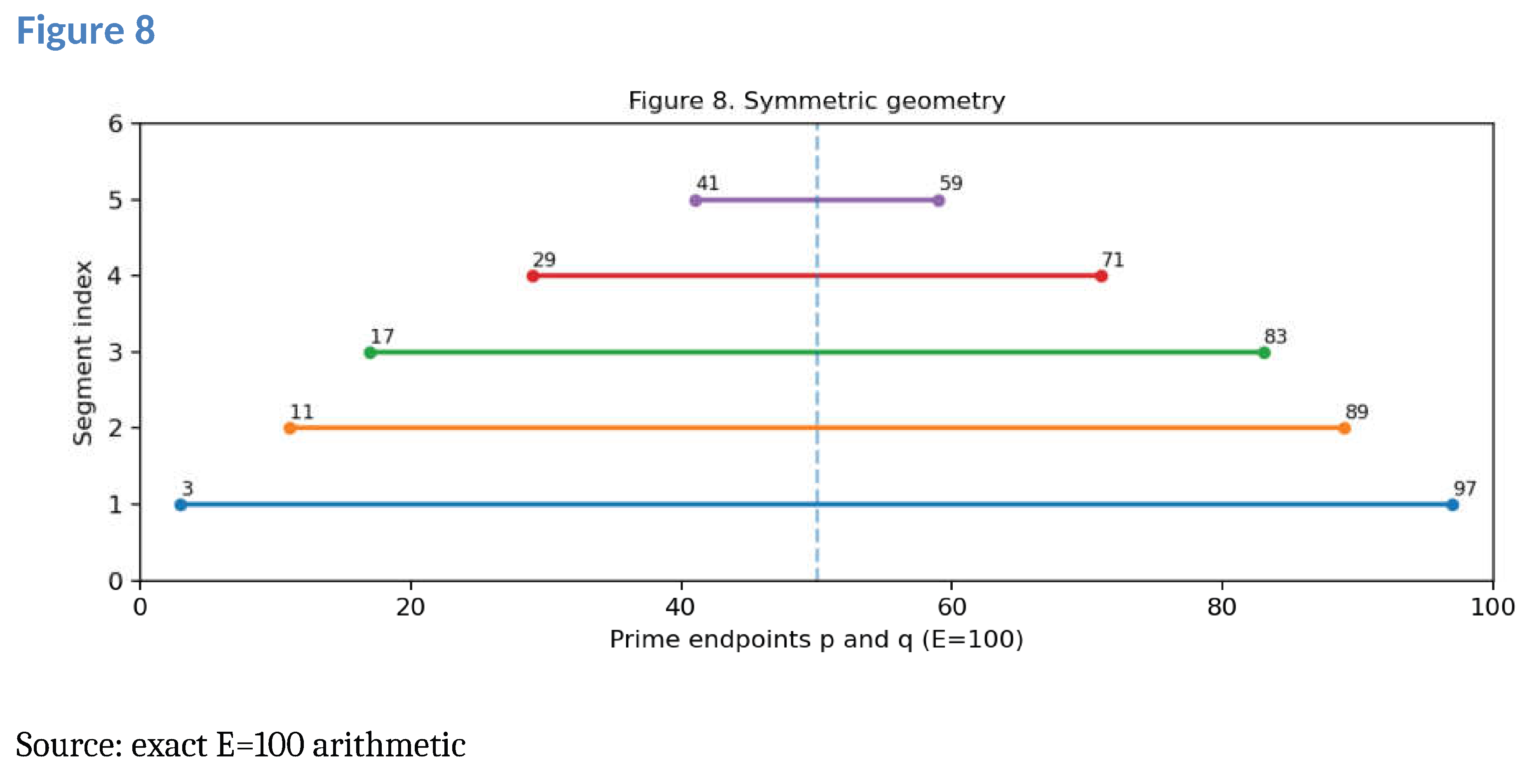
The E=100 example offers an unambiguous validation of the segment definition. Each of the five listed pairs has a prime smaller endpoint, a prime larger endpoint and sum exactly 100. The central displacement and length can be checked directly. For example, (41,59) gives m=50, d=9 and L=18; (3,97) gives d=47 and L=94. Thus increasing the peripheral distance increases segment length linearly.
Table 2 deliberately uses a small target to separate the mathematical construction from the complexities of high-precision primality testing. These rows are exact and do not depend on the large supplementary dataset. Figures 7 and 8, by contrast, are explanatory geometric schematics, not empirical endpoint-distribution plots.
8. Synchronization Chains, Ruptures, and Fresh Anchors
Figure 10 shows how repeated reuse of a fixed endpoint can form a finite chain as E advances by steps of two. Figure 9 gives the algebraic update underlying each step. A chain breaks whenever the moving endpoint becomes composite; a fresh anchor must then be sought, and the failure of one chain does not imply failure of Goldbach for the new target.
A synchronization chain is a sequence of consecutive even targets in which a designated prime endpoint is retained and the other endpoint is updated by two. A chain of length r under the k=1 rule has moving endpoints p,p+2,…,p+2r, all prime, with the fixed complement q. Since three consecutive odd numbers separated by two cannot all be prime unless one is 3, sustained q-preserving chains are severely constrained. Indeed, any three values p,p+2,p+4 include a multiple of 3; if all three are prime, the multiple must equal 3, forcing p=3. Hence a chain of three moving prime endpoints can only be 3,5,7. This elementary obstruction is critical when interpreting synchronization “persistence”.
An analogous restriction applies to the k=0 rule. Therefore the endpoint-preserving mechanism is useful as a short local shortcut, not as a source of indefinite propagation. A fresh anchor is required when all proposed continuations fail. This does not imply that Goldbach fails for the next target; it only indicates failure of a specific transition operator.
The data permit counts of candidate reuses between adjacent sampled targets, but any apparent rate depends on the available set of source representations and the chosen p-window. Table 9 summarizes observed fixed-q reuse, and Table 10 lists exact reuse examples; neither establishes a universal transition probability. Table 11 contrasts exploratory large-number candidates and the corresponding limits of primality certification.
9. Prediction Versus Search: What Can Be Measured?
Figure 9 provides the exact candidate-generation rule, whereas Figure 10 illustrates the distinct question of whether that rule reduces actual work. The relevant performance metric is the total number and cost of primality tests, including anchor discovery, rather than the percentage of targets admitting at least one endpoint-reuse transition.
A prediction should be evaluated prospectively. Before computing the representations of E+2, the algorithm receives only the verified or PRP-tagged representations of E and its fixed configuration. It then proposes candidate pairs and records whether they succeed. The success metric is not merely whether the sum identity holds—this is guaranteed algebraically—but whether the moving endpoint is prime and how much work is saved compared with a baseline.
Three distinct metrics are necessary: (i) transition success, the fraction of adjacent even targets with at least one valid endpoint-reuse continuation; (ii) minimal-p recovery, the fraction for which a predicted pair achieves the true P_min(E+2), when P_min has actually been established by exhaustive ascending search; and (iii) speedup, the ratio of computational work with and without reuse. These measures answer different questions and must not be conflated.
For k=1, a positive primality test on p+2 can replace a fresh strong test on q, which may be expensive at 1000–2000 digits. Nevertheless, this saving can be offset by the cost of maintaining a large pool of source representations or by frequent re-anchoring. A sound benchmark must account for these overheads. Figure 10 shows conditional propagation of a fixed endpoint through successive even targets; Table 9 provides the observed reuse information and Table 8 the unequal experimental scale counts.
10. Large-Integer Exploratory Cases up to 2000 Digits
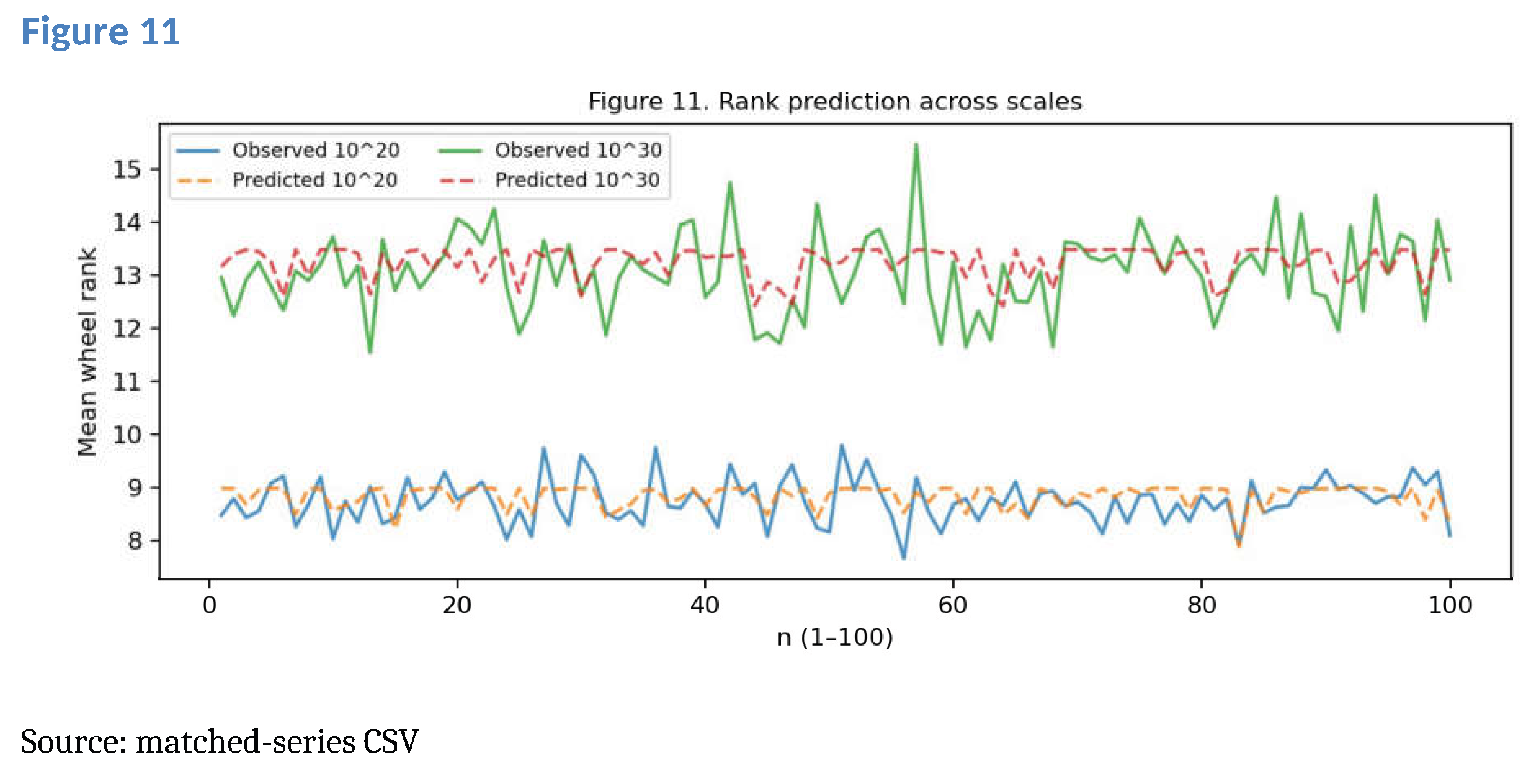
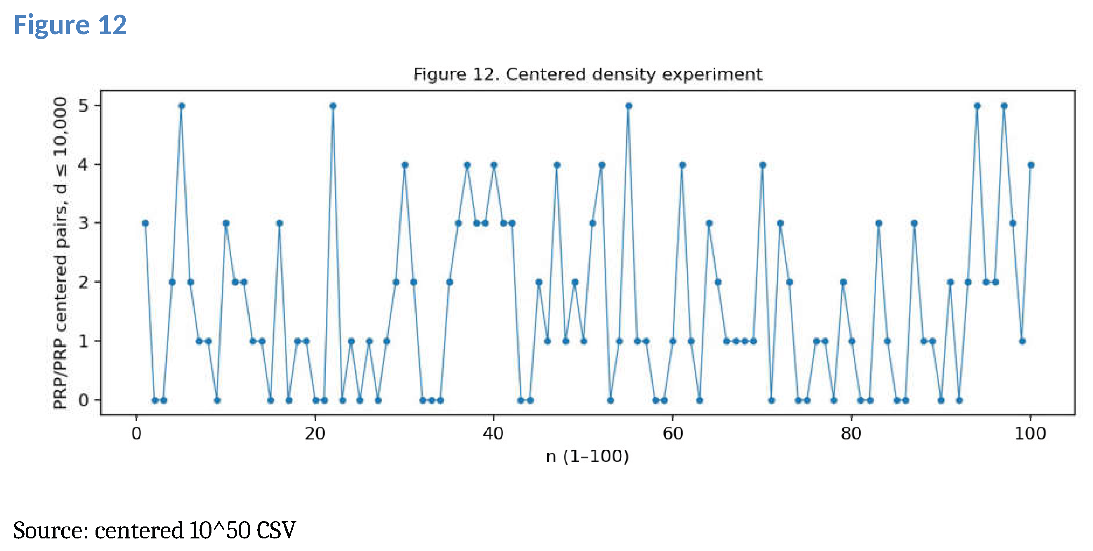
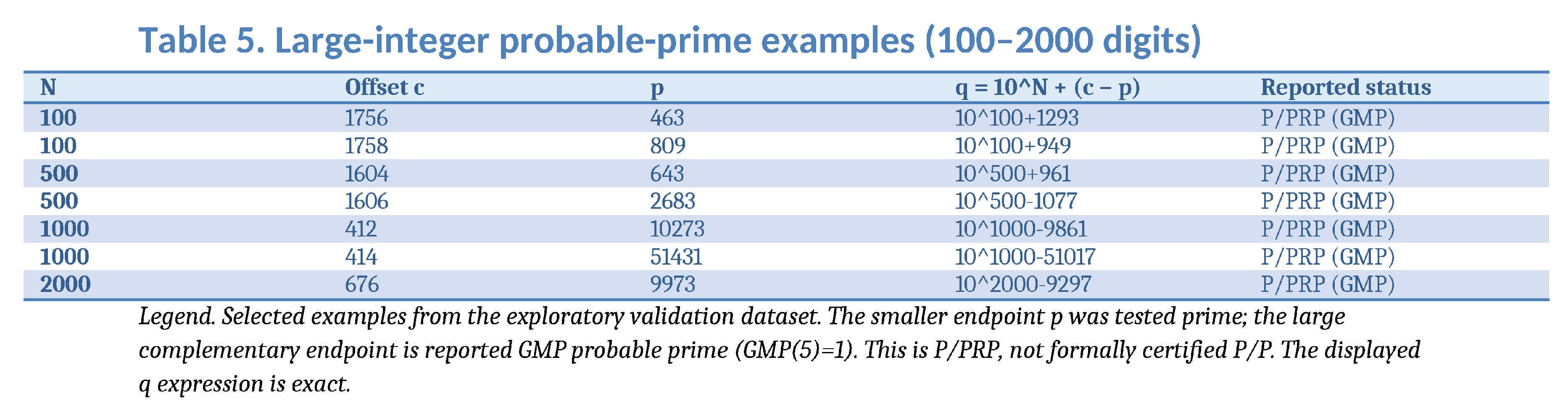
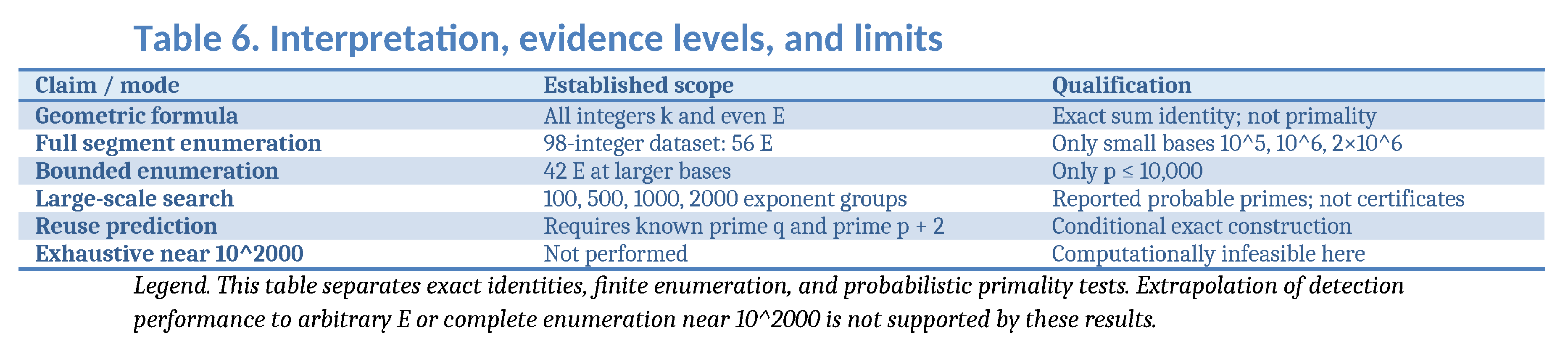
Figure 11 in the revised supplementary artwork compares the recorded matched-series observations and predictions at 10^20 and 10^30. The earlier schematic example near 10^12 is superseded in the revised figure file. Figure 12 illustrates a symbolic segment near 10^2000. Tables 5 and 11 summarize reported large-number probable-prime candidates, and Table 6 distinguishes evidence levels. Neither figure certifies primality.
For large symbolic targets of the form E = 10^N + c, the exact identity p + (10^N + c − p) = E is immediate. The nontrivial computational step is testing the second summand. The cost of that step grows with N, whereas checking whether a previously verified small p can be advanced by two is comparatively inexpensive.
A separate exploratory file reports sixteen candidate representations for target exponents N=100,500,1000 and 2000, with five candidates at each of the first three scales and one at the last. Each row records the small prime p, a symbolic large complement q=10^N+a, and a positive GMP probable-prime indicator. A later record reports positive Baillie–PSW-style checks for the same sixteen complements. These are reported computational outcomes; the current article does not supply independent primality certificates for the large q values. Table 5 records the large-integer candidates and their reported probable-prime status.
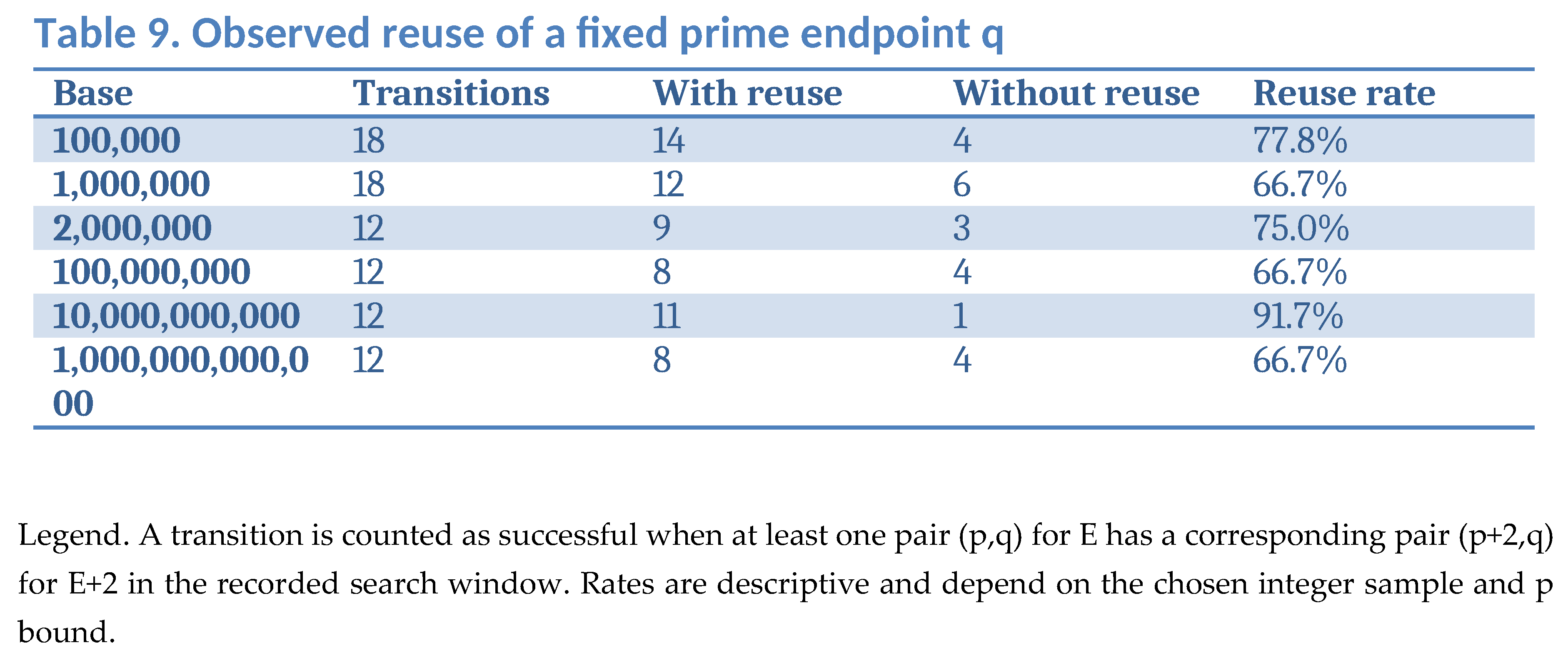
Legend. A transition is counted as successful when at least one pair (p,q) for E has a corresponding pair (p+2,q) for E+2 in the recorded search window. Rates are descriptive and depend on the chosen integer sample and p bound.
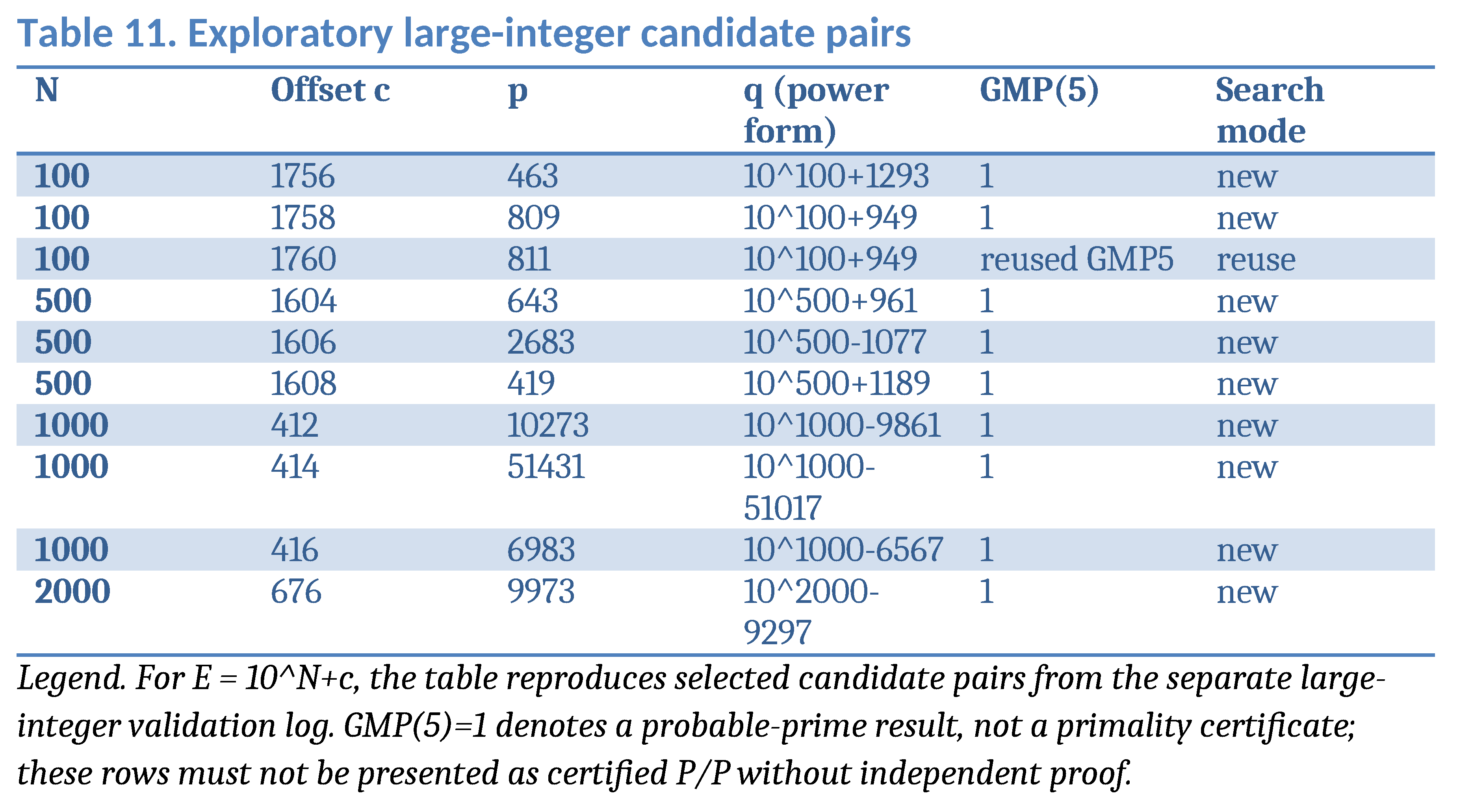
One illustrative target is E=10^2000+676, with p=9973 and q=10^2000−9297. The sum identity is exact. The designation P/PRP is retained because a probable-prime result is not a formal proof of primality. Similarly, an apparent endpoint-reuse transition between two large targets preserves the previously established PRP status but does not upgrade it to a certified prime.
As a practical matter, finding one candidate pair near 10^2000 is different from enumerating every segment: exhaustive enumeration would require examining prime p up to E/2, which is infeasible at this scale. Figure 12 visualizes the symbolic scale of the reported candidate, while Tables 5 and 11 record its exploratory P/PRP status and Table 12 describes the associated computational limitations.
11. Sieve Design and Arithmetic Constraints
Before applying an expensive primality test to q=E−p, the algorithm should eliminate candidates divisible by small primes r. The modular condition q≡0 (mod r) is equivalent to p≡E (mod r). Except when q=r itself, such a candidate is composite. This rule is exact and supports a wheel sieve, residue-lane partitioning and batch modular arithmetic. Standard sieve literature [14,15,16] explains both the efficiency and the limits of such filtering.
It is important to avoid over-interpreting sieve survivors. A large q that has no small prime factor may still be composite, including a product of two large primes. Chen’s result [3] and the general parity barrier illustrate why sieving alone does not separate primes from semiprimes in a way sufficient to prove binary Goldbach. Our pipeline therefore distinguishes SIEVE-SURVIVOR, PRP and CERTIFIED statuses.
The algorithm also records the full modular prefilter policy, its upper bound, the number of candidates entering each stage, and the test implementation. Without such metadata, reported speedups are not reproducible and can be distorted by changes in sieve depth.
12. A Falsifiable Statistical Prediction Model
The geometric map d′=d+1−2k is deterministic and contains no probabilistic information about primality. A genuine prediction model must specify how k is selected before examining the primality of the resulting endpoints. One candidate design is a score based on residue admissibility, distance from the midpoint, local prime density and previous transition outcomes. Scores should be trained on one subset of target families and evaluated on disjoint exponents or offsets.
A baseline model can rank p in ascending order and apply the same modular sieve; a second baseline can sample admissible p uniformly within the window. The proposed synchronization model should be compared against both. The primary endpoint is a reduction in strong primality tests or runtime at a fixed probability of finding a representation. Calibration curves, bootstrap uncertainty intervals and held-out test sets would be more informative than a single apparent success percentage.
For a fixed prime q, the k=1 transition succeeds precisely when p+2 is prime. Thus the elementary predictor is a twin-prime detector at the moving endpoint. Its success rate depends on the sampling protocol and local congruence structure; it cannot be assumed to remain constant as E grows. This dependence provides a testable hypothesis rather than a proof.
13. Limitations, Threats to Validity, and Proof Status
Tables 6 and 12 distinguish evidence levels, mathematical guarantees, and computational limits. First, the 304,259-row dataset is a collection of recorded computational results, not an independently certified census. Its small-base exhaustivity flags were checked by a clean rerun using independent prime enumeration; further cross-platform replication is desirable. Second, the sample includes unequal numbers of targets and unequal search windows across base scales, so raw counts are not directly comparable as rates. Third, endpoint-reuse indicators may depend on whether the preceding target was included in the same sampled block.
Fourth, the exploratory 100–2000-digit examples are P/PRP where q has not been accompanied by a formal primality certificate. The report of a BPSW positive result is strong computational evidence but not a mathematical proof. Fifth, the two elementary endpoint-preserving rules are sharply limited by the arithmetic of primes separated by two; they should not be extrapolated into long unrestricted chains.
Finally, neither the segment formalism nor the transition identity resolves the existence question for arbitrary even integers. The binary Goldbach conjecture remains open. A proof would require a new uniform existence argument, not merely the observation that already-known representations can sometimes be transformed into neighboring ones.
14. Reproducibility and Data Availability
The supplementary file S1 contains the recorded prime-pair segments and is cited throughout as the underlying dataset. Tables 3, 7 and 8 describe dataset scope and enumeration counts, while Table 2 supplies an exact small-integer control. Figures 1–10 are geometric or transition illustrations; Figure 11 presents the matched-series 10^20/10^30 comparison, and Figure 12 concerns a reported large-number candidate. Any quantitative plot should be regenerated directly from the published machine-readable files. New bounded-window experiments and rank analyses are reported in Section 17 and supplementary data S2–S5.
Supplementary File S1 is provided as a CSV file suitable for Microsoft Excel. Its 304,259 rows include the base, block identifier, rank, offset c, even target E, endpoints p and q, central distance, segment length, endpoint-reuse flag, declared coverage status and upper bound on p. The dataset should be archived alongside the code, software versions, random seed and full test logs. A supplementary validation CSV reports the sixteen large-number candidates with symbolic q expressions and probable-primality indicators.
For each row, a minimal independent audit checks that E is even, p≤q, p+q=E, d=E/2−p, and L=q−p=2d. For targets within deterministic primality ranges, both endpoints should be rechecked with an independent exact test. For enormous targets, positive PRP reports should be retained as PRP unless a certificate is available. The supplementary data are not a substitute for such an audit.
The separately prepared figures include exact finite examples, conceptual diagrams, and symbolic large-number illustrations. Figure 11 uses the recorded matched-series CSV; its quantitative interpretation remains subject to independent verification of the underlying probable-prime computations. All schematic figures must be labeled as such. Figures 1–12 and Tables 1–12 are cited in the text and supplied together as Supplementary File S6, rather than appended to the main text.
15. Discussion and Future Work
Figures 1, 2, 4, 7 and 8 explain the centered-segment geometry; Figures 3, 5, 9 and 10 depict conditional endpoint propagation; Figures 6 and 12 illustrate symbolic large-integer cases; and Figure 11 presents the recorded matched-series comparison at 10^20 and 10^30. Tables 1–2 define the framework and finite control; Tables 3, 7 and 8 describe dataset coverage; Tables 4, 9 and 10 concern endpoint reuse; and Tables 5, 6, 11 and 12 describe large-number candidates, evidence levels and limitations. None of these displays proves binary Goldbach.
The segment representation organizes Goldbach decompositions into a common geometric coordinate system and makes explicit how candidate pairs move when the target increases by two. Its chief algorithmic attraction is the possibility of reusing one already tested endpoint. This is a practical computational shortcut, not a new primality theorem. The method’s effectiveness is expected to depend on the density of admissible endpoints, the cost of large-number tests and the frequency of re-anchoring.
Further work should first implement a fully reproducible deterministic census at manageable E, then run blinded comparisons on matched target sets with identical search windows and modular filters. For large N, experiments should report the proportion of candidates passing the sieve, the number of PRP tests, the time per test, the reuse success rate and the frequency of new anchors. A clear stopping rule is essential to prevent misleading comparisons when the cost per candidate rises.
One promising extension is to generalize beyond k=0 and k=1 while penalizing changes that require two new expensive primality tests. Such a model can rank k by local arithmetic constraints and test the best candidates first. It remains necessary to measure whether the ranking performs better than ordinary sieved enumeration. This would turn a geometric identity into a quantitatively testable search strategy.
16. Conclusions
We have defined Goldbach prime-pair segments, established an exact synchronization map for neighboring even targets and identified the conditions under which an endpoint can be reused. The map is scale independent as an algebraic identity; its computational benefit is conditional on primality of the updated endpoint. A supplementary dataset of 304,259 recorded segments and a separate exploratory series up to exponent 2000 provide a basis for further experiments, subject to the stated validation limits.
The immediate scientific contribution is therefore a transparent computational framework with explicit status labels, finite examples and falsifiable benchmarking criteria. We do not claim exhaustive coverage of very large integers, a universally successful prediction rule or a proof of the binary Goldbach conjecture.
17. Extended Experiments: Wheel-Rank Prediction and Central Segment Density (19 October 2026)
The original segment geometry, exact endpoint-transition map, dataset, references and Appendices A–C are retained. The following experiments extend—not replace—the original results. Supplementary Tables 1–12 retain their original numbering; the new results are supplied as Supplementary Data S2–S5 and discussed here to avoid renumbering the twelve original tables.
17.1. Rank Gaps Between Consecutive Goldbach Segments
For a fixed even E, order the recorded pairs (p_i,E−p_i) by increasing p_i. Their segment lengths are x_i=E−2p_i, hence x_i−x_(i+1)=2(p_(i+1)−p_i) exactly. A wheel of modulus M=30030 removes candidate complements divisible by 2, 3, 5, 7, 11 or 13. Define k_i as the number of wheel-admissible candidate positions from one successful pair to the next, under the recorded enumeration convention. The rank is not a deterministic prediction of the next prime pair.
For the thirteen earlier E targets around 10^9–10^12, the rank distributions were compared with a geometric model. The finite goodness-of-fit tests did not reject that baseline at the 5% threshold; this is not a proof of independence, nor a universal law. The fitted mean-rank scaling is approximately logarithmic in E, with E-dependent local factors.
17.2. Extreme Gaps at E=10^18+46478
Within the bounded p≤10^6 search, 5,081 pairs were recorded and 5,080 between-pair intervals measured. The observed mean rank was approximately 7.958 and the maximum rank 70. Two rank-70 chains connect p=130411 to 131899 and p=330241 to 332069, respectively; the corresponding exact changes in segment length are 2,976 and 3,656. Their identical wheel ranks but different geometric lengths show that rank and Euclidean segment displacement must be reported separately. The complement primality at this size was checked computationally; the experiment is finite and does not establish a global extremum.
17.3. Two Matched Series at 10^20 and 10^30
For E_n=10^20+2n (1≤n≤100) with the same p≤100000 bound and wheel M=30030, the source records 42,305 probable-prime pair detections; the mean of the 100 observed per-target rank means is 8.7508, versus 8.8389 predicted. The per-target absolute mean error is 0.3000. These 200 matched targets form a useful scaling comparison, not an independent primality certification.
For E_n=10^30+2n (1≤n≤100) with the same p≤100000 bound and wheel M=30030, the source records 28,346 probable-prime pair detections; the mean of the 100 observed per-target rank means is 13.0530, versus 13.2593 predicted. The per-target absolute mean error is 0.5532. These 200 matched targets form a useful scaling comparison, not an independent primality certification.
17.4. Centered Pairs at 10^50
For E_n=10^50+2n (1≤n≤100), m_n=E_n/2 and candidate half-length 1≤d≤10000, the file records 159 probable-prime pairs across 1,000,000 tested offsets and 71 targets with at least one detection. The empirical raw frequency is 0.000159 per offset; this is a finite-window frequency, not an unconditional density theorem. For n=1, the first recorded half-length is d=1352. The identity p=m−d, q=m+d ensures the midpoint is exactly E/2 for every representation.
17.5. Singular-Series Baseline and Its Limits
Let S(E)=2 C_2 ∏_(r|E,r>2) (r−1)/(r−2), where C_2=∏_(r>2)(1−1/(r−1)^2). This classical Hardy–Littlewood singular series suggests the heuristic central expectation R(E,H)≈H S(E)/log(E/2)^2 for H much smaller than E. This estimate is not a proven uniform lower bound for polylogarithmic H. The previous wheel model estimates mean rank by alpha_M(E) log(E)/S(E), with alpha_M(E)=∏_(r|M,r>2,r∤E)(r−2)/(r−1), and is conditional on the wheel convention and prime-candidate sampling. A position-varying hazard may be written s_j≈min(1,S(E)/(alpha_M(E)log(E−a_j))) and P(k≤h)≈1−∏_(j=1)^h(1−s_j). Its product form assumes conditional independence and must be validated on held-out targets; it is not an exact identity.
17.6. Mathematical Status and Falsifiability
The midpoint and segment-difference identities are exact. The experimental pair counts and rank summaries are finite computational records. For 20-, 30- and 50-digit complements, probable-prime labels must not be silently promoted to formally certified primes. Failure to find a centered pair with d≤H is not a counterexample to Goldbach. A proof would require a uniform positivity result R(E,H(E))>0 for every sufficiently large even E, with a rigorously admissible window H(E)<E/2. Future tests should pre-register training/holdout splits, compare calibration and tail errors, and publish exact primality certificates when possible.
Extended data files: S2, thirteen-target geometric residual audit; S3, E=10^18+46478 segment and extreme-chain files; S4, 200 matched targets at 10^20 and 10^30; S5, 100 centered targets at 10^50. Figures 1–12 and Tables 1–12 are combined in Supplementary File S6 (Supplementary_Figures_and_Tables_1_to_12.docx). Figure 11 in S6 uses recorded matched-series data rather than the former schematic illustration. Worked examples are provided separately in Supplementary File S7.
Supplementary Materials
The following supporting information can be downloaded at the website of this paper posted on Preprints.org
Author Contributions
Conceptualization, methodology and investigation, B.B.; manuscript preparation and data visualization, assisted computational drafting. All computational claims require final author verification before submission.
Funding
No external funding was reported for this study.
Institutional Review Board Statement
Not applicable.
Informed Consent Statement
Not applicable.
Data Availability Statement
Supplementary File S1 (304,259 recorded segment rows) and associated experimental files accompany the manuscript.
Conflicts of Interest
The author declares no conflict of interest.
Appendix A. Exact Geometry and Complete Synchronization Parametrization
Appendix A.1. Definition and Bijection
Let E ≥ 4 be an even integer, and write m = E/2. Define G(E) = {(p,q): p and q are prime, 2 ≤ p ≤ q, p + q = E}. Every pair in G(E) corresponds uniquely to an integer d ≥ 0 satisfying p = m − d and q = m + d. Conversely, every integer d ≥ 0 for which m − d and m + d are primes and m − d ≥ 2 yields one pair in G(E). Thus G(E) is in bijection with the set D(E) = {d ∈ Z: 0 ≤ d ≤ m − 2, m − d and m + d prime}. The geometric segment is the closed interval [m − d, m + d], whose length is exactly 2d.
Appendix A.2. Theorem: Complete Algebraic Transition
Theorem A1. Let E be even, (p,q) ∈ G(E), and E′ = E + 2. Every integer pair (p′,q′) satisfying p′ + q′ = E′ and p′ ≡ p (mod 2) has a unique integer k such that p′ = p + 2k and q′ = q + 2 − 2k. Its centered displacement satisfies d′ = d + 1 − 2k, where d = E/2 − p and d′ = E′/2 − p′. Conversely, each k ∈ Z yields the sum identity; it yields a Goldbach segment precisely if p′ and q′ are prime and 2 ≤ p′ ≤ q′.
Proof. The parity hypothesis gives k = (p′ − p)/2 ∈ Z, uniquely. Substituting p′ into p′ + q′ = p + q + 2 gives q′ = q + 2 − 2k. Since E′/2 = E/2 + 1, d′ = (E/2 + 1) − (p + 2k) = d + 1 − 2k. The converse follows by addition. The prime and ordering requirements are separate and cannot be inferred from the sum identity. QED.
Remark. For odd-prime pairs at even E > 4, the parity hypothesis is automatic. The exceptional pair involving 2 occurs only at E = 4 (2 + 2); it must be treated explicitly when applying parity-restricted transitions. The parametrization is complete for ordered odd-prime endpoint pairs, but it is not itself a primality prediction.
Appendix A.3. Two Endpoint-Preserving Corollaries
Corollary A1. Under k = 1, q′ = q and p′ = p + 2; a valid continuation exists if and only if p + 2 is prime. Under k = 0, p′ = p and q′ = q + 2; a valid continuation exists if and only if q + 2 is prime. The respective displacement changes are d′ = d − 1 and d′ = d + 1, subject to the ordering convention. Proof: substitute k = 1 or k = 0 into Theorem A1 and apply the primality condition. QED.
Appendix B. Arithmetic Obstructions, Exact Counts, and Algorithmic Correctness
Appendix B.1. Local Congruence Obstruction
Lemma A2. Let r be prime, E even, and p prime with q = E − p > r. If p ≡ E (mod r), then q is composite. Proof. The congruence gives r | q. Because q > r, q has a nontrivial divisor r and is composite. QED. This provides a rigorous exclusion rule for the sieve. The exception q = r is essential.
Appendix B.2. Maximum Length of an Endpoint-Preserving Chain
Proposition A2. Suppose q is held fixed and p, p + 2, …, p + 2t are all primes, where p is odd and t ≥ 2. Then p = 3 and t = 2; the moving endpoints are exactly 3, 5, 7. In particular, no fixed-q synchronization chain can contain four successive even targets. Proof. Among p, p + 2, p + 4 exactly one is divisible by 3. If all three are prime, that term must be 3. Since p ≥ 3, necessarily p = 3. The next value p + 6 = 9 is composite. QED. The same argument applies when p is fixed and q increases by two.
Corollary A2. No iteration of the elementary k = 0 or k = 1 endpoint-preserving rule alone can prove Goldbach by indefinite propagation. It must be supplemented by a new-anchor existence mechanism. This is an exact structural limitation, not an observed statistical dispersion.
Appendix B.3. Exact Finite Representation Count
Define 1_P(n) to equal 1 if n is prime and 0 otherwise. The number of unordered Goldbach representations of E is R(E) = Σ_{2 ≤ p ≤ E/2} 1_P(p)1_P(E − p), with the sum over integers p. Equivalently, R(E) = |D(E)|. Goldbach for E is equivalent to R(E) ≥ 1. A complete finite census at E evaluates this sum using an exact primality test for every candidate p (or an equivalent complete sieve); a search restricted to p ≤ H < E/2 evaluates only R(E;H) and cannot certify R(E) exactly.
Appendix B.4. Soundness and Completeness of the Algorithm
Theorem A3 (soundness). If the algorithm emits (p,q) only after verifying p + q = E and obtaining valid primality proofs for both endpoints, every emitted CERTIFIED pair belongs to G(E). Proof. This is immediate from the definition of G(E). QED. A PRP-tagged output does not satisfy the premise and must not be counted as a certified theorem.
Theorem A4 (bounded completeness). Suppose the algorithm enumerates every prime p ≤ H with p ≤ E/2 and applies an exact test to q = E − p without erroneous exclusions. Then its certified output equals G_H(E) = {(p,q) ∈ G(E): p ≤ H}. Proof. Soundness gives one inclusion. For the other, each (p,q) ∈ G_H(E) has p in the enumeration; the exact q test accepts it, so it is emitted. QED. Full completeness holds only when H ≥ E/2.
Appendix C. Exact Reduction Toward the Binary Goldbach Existence Problem
Appendix C.1. Positivity Is the Unresolved Mathematical Target
For even E ≥ 4, let R(E) = Σ_{2 ≤ p ≤ E/2} 1_P(p)1_P(E − p). The binary Goldbach conjecture is equivalent to the statement R(E) > 0 for every even E ≥ 4. A uniform estimate R(E) ≥ 1 for all sufficiently large even E, together with exact verification of the finitely many smaller cases, would prove the conjecture. This equivalence is a reduction of the goal, not progress toward proving the required lower bound.
Appendix C.2. Chen-Supported Liouville Separation: An Exact Identity
Define the Liouville function λ(n) = (−1)^{Ω(n)}, where Ω(n) counts prime factors with multiplicity. Let P2 denote integers with exactly two prime factors counted with multiplicity. For a fixed even E, choose any nonnegative weight w_E(p) supported on primes p with q = E − p belonging to P ∪ P2, and count each unordered candidate at most once (p ≤ E/2). Define C(E) = Σ_p w_E(p) and L(E) = Σ_p w_E(p) λ(E − p). Then (C(E) − L(E))/2 = Σ_{p: E−p prime} w_E(p), because λ(q) = −1 for primes and λ(q) = +1 for q ∈ P2. This is an exact weighted prime-selection identity under the stated support condition.
Proof. Split the support into the disjoint sets q ∈ P and q ∈ P2. On the first set 1 − λ(q) = 2, and on the second set 1 − λ(q) = 0. Therefore (C − L)/2 = Σ_p w_E(p)(1 − λ(E − p))/2 = Σ_{q prime} w_E(p). QED.
Appendix C.3. Conditional Uniform-Positivity Theorem
Theorem A5 (conditional). Suppose there exists E0 such that, for every even E ≥ E0, one can construct nonnegative weights w_E supported as above for which C(E) − L(E) > 0. Suppose additionally that all even E with 4 ≤ E < E0 have a verified Goldbach representation. Then the binary Goldbach conjecture follows. Proof. By the identity in A3.2, C(E) − L(E) > 0 implies the existence of at least one prime q = E − p with w_E(p) > 0; the support requires p prime. Smaller cases are handled by the finite verification. QED.
The missing step is precisely the uniform strict inequality C(E) − L(E) > 0, with effective control of the parity-sensitive Liouville term. Chen-type support alone does not establish it. The synchronization identities in Appendix A do not supply it either. Any future proof must establish a new uniform non-cancellation or non-avoidance estimate, not infer it from finite experiments or from the fact that an algebraic transition preserves sums.
Appendix C.4. Relation to Windowed Prediction
For a search window H(E), define R(E;H) = Σ_{2 ≤ p ≤ min(H(E),E/2)} 1_P(p)1_P(E − p). The condition R(E;H) > 0 is equivalent to the existence of a Goldbach pair with smaller prime endpoint at most H(E). A theorem proving this positivity uniformly would be stronger than mere numerical success of the algorithm. No unconditional uniform positivity theorem at the logarithmic windows considered in this research is established here. The synchronization score may prioritize candidates but cannot substitute for this missing analytic estimate.
Mathematical status summary: Appendix A and Appendix B contain exact elementary identities and finite correctness statements; Appendix C.2 is an exact identity under explicit Chen-type support; Theorem A5 is conditional; the uniform positive lower bound needed for a proof remains open. These distinctions must be preserved in all subsequent revisions.
References
- Hardy, G.H.; Littlewood, J.E. Some problems of “Partitio Numerorum”; III: On the expression of a number as a sum of primes. Acta Math. 1923, 44, 1–70. [Google Scholar] [CrossRef]
- Vinogradov, I.M. Representation of an odd number as a sum of three primes. Dokl. Akad. Nauk SSSR 1937, 15, 291–294. [Google Scholar]
- Chen, J.R. On the representation of a large even integer as the sum of a prime and the product of at most two primes. Sci. Sin. 1973, 16, 157–176. [Google Scholar]
- Helfgott, H.A. The ternary Goldbach conjecture is true. arXiv 2013, arXiv:1312.7748. [Google Scholar]
- Helfgott, H.A. Major arcs for Goldbach’s problem. arXiv 2013, arXiv:1305.2897. [Google Scholar]
- Helfgott, H.A. Minor arcs for Goldbach’s problem. arXiv 2012, arXiv:1205.5252. [Google Scholar]
- Oliveira e Silva, T.; Herzog, S.; Pardi, S. Empirical verification of the even Goldbach conjecture and computation of prime gaps up to 4 × 10^18. Math. Comput. 2014, 83, 2033–2060. [Google Scholar]
- Helfgott, H.A.; Platt, D.J. Numerical verification of the ternary Goldbach conjecture up to 8.875 × 10^30. Exp. Math. 2013, 22, 406–409. [Google Scholar]
- Ramaré, O. On Šnirel’man’s constant. Ann. Sc. Norm. Super. Pisa Cl. Sci. 1995, 22, 645–706. [Google Scholar]
- Deshouillers, J.-M.; Effinger, G.; te Riele, H.; Zinoviev, D. A complete Vinogradov 3-primes theorem under the Riemann hypothesis. Electron. Res. Announc. Am. Math. Soc. 1997, 3, 99–104. [Google Scholar] [CrossRef]
- Montgomery, H.L.; Vaughan, R.C. The exceptional set in Goldbach’s problem. Acta Arith. 1975, 27, 353–370. [Google Scholar] [CrossRef]
- Vaughan, R.C. The Hardy–Littlewood Method, 2nd ed.; Cambridge University Press: Cambridge, UK, 1997. [Google Scholar]
- Iwaniec, H.; Kowalski, E. Analytic Number Theory; American Mathematical Society: Providence, RI, USA, 2004; Volume 53. [Google Scholar]
- Halberstam, H.; Richert, H.-E. Sieve Methods; Academic Press: London, UK, 1974. [Google Scholar]
- Greaves, G. Sieves in Number Theory; Springer: Berlin/Heidelberg, Germany, 2001. [Google Scholar]
- Bombieri, E. On the large sieve. Mathematika 1965, 12, 201–225. [Google Scholar] [CrossRef]
- Goldston, D.A.; Pintz, J.; Yıldırım, C.Y. Primes in tuples I. Ann. Math. 2009, 170, 819–862. [Google Scholar] [CrossRef]
- Zhang, Y. Bounded gaps between primes. Ann. Math. 2014, 179, 1121–1174. [Google Scholar] [CrossRef]
- Maynard, J. Small gaps between primes. Ann. Math. 2015, 181, 383–413. [Google Scholar] [CrossRef]
- Polymath, D.H.J. Variants of the Selberg sieve, and bounded intervals containing many primes. Res. Math. Sci. 2014, 1, 12. [Google Scholar] [CrossRef]
- Gallagher, P.X. On the distribution of primes in short intervals. Mathematika 1976, 23, 4–9. [Google Scholar] [CrossRef]
- Cramér, H. On the order of magnitude of the difference between consecutive prime numbers. Acta Arith. 1936, 2, 23–46. [Google Scholar] [CrossRef]
- Granville, A. Harald Cramér and the distribution of prime numbers. Scand. Actuar. J. 1995, 1995, 12–28. [Google Scholar] [CrossRef]
- Dusart, P. Estimates of some functions over primes without R.H. arXiv 2010, arXiv:1002.0442. [Google Scholar]
- Rosser, J.B.; Schoenfeld, L. Approximate formulas for some functions of prime numbers. Ill. J. Math. 1962, 6, 64–94. [Google Scholar] [CrossRef]
- Pomerance, C. A tale of two sieves. Not. Am. Math. Soc. 1996, 43, 1473–1485. [Google Scholar]
- Miller, G.L. Riemann’s hypothesis and tests for primality. J. Comput. Syst. Sci. 1976, 13, 300–317. [Google Scholar] [CrossRef]
- Rabin, M.O. Probabilistic algorithm for testing primality. J. Number Theory 1980, 12, 128–138. [Google Scholar] [CrossRef]
- Baillie, R.; Wagstaff, S.S., Jr. Lucas pseudoprimes. Math. Comput. 1980, 35, 1391–1417. [Google Scholar] [CrossRef] [PubMed]
- Agrawal, M.; Kayal, N.; Saxena, N. PRIMES is in P. Ann. Math. 2004, 160, 781–793. [Google Scholar] [CrossRef]

Table 12.
Scope, mathematical guarantees, and limitations.
| Claim or result | Evidence level | Qualification |
|---|---|---|
| p+q=E; m=E/w; d=m−p | Exact identity | Any even E and integer candidate endpoints |
| p′=p=2k;q′=q+2−2k | Exact sum-preserving transformation | Both new endpoints must separately be prime |
| d′=d+1−2k | Exact geometric identity | Follows from m′=m+1 |
| k=1: q′=1 | Conditional exact reuse | Requires p+2 prime; q retains its prior status |
| Small E complete enumeration | Finite exact computation | Only within reported exhaustive ranges |
| Large E GMP/BPSW positives | Probable-prime evidence | Not formal certificates |
| All segments near 10^2000 | Not established | Full enumeration computationally infeasible |
Legend. The algorithm preserves the sum and predicts candidate geometry exactly. Primality is an independent requirement. Observed transition frequencies are sample-dependent; they do not imply an unconditional proof of Goldbach’s conjecture.
Disclaimer/Publisher’s Note: The statements, opinions and data contained in all publications are solely those of the individual author(s) and contributor(s) and not of MDPI and/or the editor(s). MDPI and/or the editor(s) disclaim responsibility for any injury to people or property resulting from any ideas, methods, instructions or products referred to in the content. |
© 2026 by the authors. Licensee MDPI, Basel, Switzerland. This article is an open access article distributed under the terms and conditions of the Creative Commons Attribution (CC BY) license (http://creativecommons.org/licenses/by/4.0/).
Copyright: This open access article is published under a Creative Commons CC BY 4.0 license, which permit the free download, distribution, and reuse, provided that the author and preprint are cited in any reuse.