Modeling Maximum Extreme Values by New Different Continuous Distributions Derived from the Median Based Unit Rayleigh Distribution

Iman M. Attia

doi:10.20944/preprints202610.1883.v1

Submitted:

19 October 2026

Posted:

20 October 2026

You are already at the latest version

Abstract

The maximum extreme value is defined as the largest order statistic. It has many applications in real-world data as a measure of maximum rainfall, floods, and extremely high temperatures. Modeling these data is important to reduce the effect of disasters that may cause loss of lives and money. In this paper the author developed different distributions by applying different transformation on the variable that follows Median Based Unit Rayleigh (MBUR) distribution which is defined on the unit interval. The author explains the derivation for each distribution, illustrates the PDF, CDF, and the hazard rate function with illustrated figures. For each distribution the quantile function is also expounded. The moments are thoroughly discussed. The asymptotic limiting distribution is clarified for each distribution. According to the transformation deployed on the MBUR, two asymptotic limiting distribution were achieved, the Gumbel and the Frechet distribution. The MBUR has a Weibull asymptotic limiting distribution, which is type III of the Generalized Extreme distribution.

Keywords:

negative log squared‐MBUR

;

Frechet derived MBUR

;

negative double log parameterized MBUR

Subject:

Computer Science and Mathematics - Probability and Statistics

Introduction

Extreme Value Theory, as its name indicates, serves as a framework for modeling the extreme values, including both maximum and minimum, of random samples derived from random variables. This theory is particularly beneficial for analyzing rare events with no assumptions regarding the underlying distribution. It employs asymptotic arguments and approximations, akin to the application of the Central Limit Theorem in relation to means. In contrast to the Central Limit Theorem, which emphasizes the behavior of arithmetic averages, Extreme Value Theory focuses on the behavior of the maximum (or minimum) of these random variables as the sample size (n) approaches infinity. Additionally, it investigates the behavior of the distribution of a random variable conditioned to exceed a specified high threshold (t). In this analysis, observations below the threshold are excluded, allowing for a detailed examination of the limiting distributions of the remaining extreme observations, represented through the Peak Over Threshold method. There exist analogous limiting distributions within Extreme Value Theory, comparable to the normal distributions identified in the Central Limit Theorem. In practical applications where it is essential to concentrate on the behavior of values in the rare instances when they surpass the threshold (x > t), these limiting distributions may be utilized as models for x, thereby providing valuable insights into extreme events.

Let X₁ , X₂, …, X_n be a sequence of independent and identically distributed (i.i.d.) random variables drawn from a continuous cumulative distribution function, F(x). The sample maximum is defined M_n = max(X₁ , X₂, …, X_n). The exact distribution of M_n is given by P(M_n ≤ x) = [F(x)]ⁿ as n → ∞ . This distribution becomes degenerate if left unscaled. Studying the non-degenerate asymptotic limiting distribution requires a linear normalization defined by a scale sequence a_nand a location sequence b_n such that:

\lim_{n \to \infty} F^{n} (a_{n} x + b_{n}) = G (x)

, where G(x) is a non-degenerate distribution function. If such sequences exist, F(x) is said to belong to the Max-Domain of Attraction of (G), denoted as F ∈ D(G). By the Fisher-Tippett-Gnedenko theorem, G(x) must belong to the Generalized Extreme Value (GEV) family, taking either a Gumbel or Fréchet archetype for infinite upper-tail supports. (Fisher & Tippett, 1928)

The derivation of the normalizing sequences a_n and b_n is heavily dictated by the distribution's upper endpoint, defined as x^* = sup{x:F(x) < 1} , and the mathematical structure of its upper tail.(Kotz & Nadarajah, 2000), (De Haan & Ferreira, 2006)

Case A: Support on the Entire Real Line (−∞,+∞)

When a distribution has support spanning (−∞,+∞), its upper endpoint is infinite x^* = ∞ If the probability density function (PDF) decays at an exponential rate—such as in the Normal or Logistic distributions—the tail is considered "light". Domain of Attraction: These distributions belong to the Gumbel Domain of Attraction (D(G₀)).The sequences are typically derived using the inverse tail-quantile function. Specifically, b_n is established via b_n = 1−; in other words,

b_{n} = F^{- 1} (1 - \frac{1}{n + 1})

, while a_n acts as an auxiliary scale function evaluated at b_n, defined by

a_{n} = \frac{1 - F (b_{n})}{f (b_{n})} = \frac{1}{nf (b_{n})}

Case B: Semi-Infinite Support on (0,+∞)

For distributions restricted to the positive semi-infinite real line(0,+∞) with an infinite upper endpoint x^* = ∞, the limiting behavior branches into two distinct categories based on regular variation at infinity:

Heavy-Tailed Distributions (Fréchet Domain): If the tail decays polynomially (e.g., Pareto, Cauchy distributions), the tail is "heavy" or "fat". The survival function 1 - F(x) is regularly varying with a negative tail index −α where α > 0. These distributions fall into the Fréchet Domain of Attraction (D(G₁)). The normalization simplifies because we can set b_n = 0, and the scale sequence scales polynomially: $a_{n} = F^{- 1} (1 - \frac{1}{n + 1}) \propto n^{\frac{1}{α}}$

Medium-Tailed Distributions (Gumbel Domain): If the tail decays faster than any power law but slower than a pure exponential form (e.g., Lognormal or Gamma distributions), the support is (0,+∞), yet it converges asymptotically to a Gumbel distribution. In this sub-case, von Mises' transformation criteria must be applied to isolate the auxiliary scaling function a_n preserving $b_{n} = F^{- 1} (1 - \frac{1}{n + 1})$ .

Case C: Bounded Support from the Upper End (−∞, x^*)

When a distribution has a hard upper ceiling, its upper endpoint is finite x^* < ∞. If the probability density function (PDF) approaches this upper limit according to a power-law scaling—such as in the Uniform or Beta distributions—the tail is considered "bounded". These distributions belong to the Weibull Domain of Attraction (D(G_γ)). where the GEV shape parameter ξ = γ < 0 , or classically denoted as (D Ψ_α), and α > 0.The normalization sequences can be established in two standard ways depending on the unified GEV framework or the classical type-specific limits:

Unified GEV Representation: To mirror Case A directly, b_n is established via $b_{n} = 1 - \frac{1}{n + 1}$ in other words, $b_{n} = F^{- 1} (1 - \frac{1}{n + 1})$ , while a_n acts as an auxiliary scale function evaluated at b_n, defined by $a_{n} = \frac{1 - F (b_{n})}{f (b_{n})} = \frac{1}{nf (b_{n})}$ .
Classical Type III Representation: Because the distribution has a known maximum barrier x^* , the location sequence is frequently pinned directly to the absolute boundary, b_n = x^* , while the scaling sequence a_n tracks the shrinking distance from the high quantile to that boundary ceiling: $a_{n} = 1 - F^{- 1} (1 - \frac{1}{n + 1})$ .

The linear transformation y = a_n x + b_n is used to keep the distribution stable as n → ∞

P (\frac{M_{n} - b_{n}}{a_{n}} \leq x) = {[F (a_{n} x + b_{n})]}^{n}

If the normalizing constants of a newly proposed distribution lead to a non-degenerative limit (like the Gumbel distribution), it proves that the distribution belongs to the Gumbel Maximum Domain of Attraction (MDA).(Haan, 1976)

If it converges to a constant instead of a distribution (meaning it becomes degenerate), it cannot be used for Extreme Value Theory (EVT) modeling. Therefore, proving it converges to the Gumbel distribution is a foundational validation.

The question raised here: If the ultimate limit is just the standard Gumbel distribution anyway, what value does the new "parent" distribution actually bring?

The value does not lie in the infinite limit n → ∞ but rather in how the distribution behaves when moving toward that limit (n is finite). This can be explained in the following points:

1.Superior Penultimate Behavior (Finite n Precision)

In the real world, sample size is never infinite it is a finite dataset. The Problem with Gumbel, for example: The standard Gumbel distribution assumes a very specific, rigid rate of convergence. For many distributions (like the Normal or Log-Normal), the convergence to the Gumbel limit is notoriously slow; fitting a Gumbel distribution directly to finite data, the risk estimates will be heavily biased. The Value of New Distributions: A new distribution often contains extra parameters (shape or skewness parameters) that allow it to fit the penultimate (near-extreme) behavior of the data perfectly. It acts as a bridge, accurately capturing data behavior at finite sample sizes while remaining mathematically guaranteed to safely transition into a Gumbel distribution at true infinity.

2.Physical and Structural Interpretation

Standard extreme value distributions are purely statistical empirical models—they don't understand physics, economics, or engineering. New parent distributions are often derived from the physical mechanisms of the system itself. For example: In reliability engineering, a new distribution might be derived based on how a component degrades over time under fluctuating stress. Knowing that this physically backed distribution mathematically converges to a Gumbel distribution means engineers can trust it for extreme safety bounds, while still using its parameters to understand the physical day-to-day wear and tear.

3.Resolving the "Tail Heaviness" Ambiguity

The Gumbel domain is incredibly diverse. It includes light-tailed distributions (like the Exponential), medium-tailed distributions (like the Normal), and even distributions with log-exponential tails (like the Log-Normal). A new distribution allows researchers to model complex, hybrid tail structures that look heavy-tailed in the medium run but are ultimately light-tailed at the extreme edge. It prevents overestimating risks (which happens if a Fréchet distribution is falsely chosen) or underestimating risks (which happens if forcing a standard Exponential tail).

Proving a new distribution has a Gumbel limit is a safety check—it guarantees that the distribution behaves logically under extreme conditions. The benefit of using it over a generic Gumbel model is that it fits the realistic, non-infinite data you actually possess much better, leading to vastly more accurate real-world engineering or financial forecasts.

Direct Comparison: Direct Gumbel vs. New Parent Distribution

Feature	Direct Gumbel Fitting	New Parent Distribution (Gumbel MDA)
Data Requirement	Requires a massive dataset of block maximums.	Can be fitted to the entire dataset, preserving sample size.
Finite-Sample Accuracy	Poor if the convergence rate of the underlying process is slow.	High, because it captures the specific shape of the non-extreme data.
Parameter Flexibility	Rigid (only location and scale).	Flexible (can include shape, skewness, or hurdle parameters).
Physical Meaning	Purely statistical; describes only the absolute worst-case scenario.	Can map physical traits (e.g., crack propagation, rainfall intensity).

The Generalized Extreme Value (GEV) Distribution

The foundational formula that combines all three classic extreme value distributions (Gumbel, Fréchet, and Weibull) into a single mathematical framework is the Generalized Extreme Value (GEV) distribution.(Beirlant et al., 2004)

The Cumulative Distribution Function (CDF) of the GEV is expressed as:

H_{ξ} (x) = \exp (- {(1 + ξ (\frac{x - μ}{σ}))}^{\frac{- 1}{ξ}})

This formula is valid for the domain

1 + ξ (\frac{x - μ}{σ}) > 0

where:

μ is the location parameter, σ is the scale parameter, and ξ is the shape parameter (Extreme Value Index). It unifies the three distributions based on ξ :

ξ > 0 : Fréchet Distribution (Heavy-tailed). The tail decays polynomially (e.g., Pareto, Log-Normal, Cauchy).
ξ < 0 : Reversed Weibull Distribution (Bounded tail). The distribution has a strict finite upper bound (e.g., Uniform, Beta).
ξ = 0 : Gumbel Distribution (Light-tailed). The tail decays exponentially (e.g., Exponential, Normal, Gamma).

Any continuous distribution's largest order statistic can be mathematically mapped to one of these three target families by using the normalization sequences a_n and b_n by setting the baseline CDF equal to a function of the sample expectation, like n/(n + 1).

Mood, Graybill, and Boes, (Mood et al., 1974) used a universal method to find the centering normalizing constant b_n . Because the Probability Integral Transform dictates that plugging any continuous random variable into its own CDF yields a standard Uniform distribution F(x)~U(0,1), and the expected value of a standard uniform maximum is n/(n+1), the authors used n/(n+1) as a universal target percentile to find b_n for any population distribution.

Steps to find the asymptotic limiting distribution of the extreme value

Step 1: Find the Centering Sequence b_n.

Map the sample maximum via probability integral transform to evaluate the tail quantile. Set the population or parent CDF equal to the expected value of the standard uniform maximum to isolate the b_n. For heavy-tailed distributions, b_n grows very slowly at a polynomial rate. For the light-tailed distribution, b_n grows at a much faster exponential rate.

Step 2: Determine the Scaling Sequence a_n.

For heavy-tailed distributions, the extreme values stretch out proportionally to the centering constant itself. Therefore, the scaling factor matches the growth rate of the center. This rule can be applied for some light-tailed distribution as will be shown in section 2.

Step 3: Substitute linear transformation into the Population or the parent CDF.

Substitute the linear transformation into the parent CDF with the calculated a_n and b_n

Step 4: Evaluate the Asymptotic Limit.

Examine the weak convergence of the linearly transformed parent distribution as (n) approaches infinity. To find the limiting distribution of the maximum, raise this transformed CDF to the power of (n) and take the limit as n → ∞.

If the distribution has a heavy, power-law tail, its maximum values don't cluster tightly together as they do in the light-tailed distributions; the polynomial scaling sequence a_n accommodates massive, volatile jumps, which naturally transforms the limit into a Fréchet distribution instead of a Gumbel.

Necessary and Sufficient Conditions (Domains of Attraction)

For a continuous cumulative distribution function F(x) with an upper endpoint x^* = sup{x:F(x) < 1}the necessary and sufficient conditions for F to belong to the Maximum Domain of Attraction (MDA) of the Gumbel and Fréchet distributions are outlined below.(Leadbetter et al., 1983)

Fréchet Distribution (Type II):

The Fréchet distribution applies to heavy-tailed distributions with an infinite upper endpoint x_F = ∞ . F belongs to the MDA of the Fréchet distribution if and only if x_F = ∞ and the tail 1 - F(x) is regularly varying at infinity with a negative index α where α > 0

Mathematical Expression:

\lim_{t \to \infty} \frac{1 - F (tx)}{1 - F (t)} = x^{- α} for all x > 0

Gumbel Distribution (Type I):

The Gumbel distribution applies to light-tailed distributions (e.g., Normal, Exponential, Gamma) where the tail decreases exponentially fast. The upper endpoint F_x can be finite or infinite. F belongs to the MDA of the Gumbel distribution if and only if there exists a positive auxiliary function g(t) such that for all real x:

Mathematical Expression:

\lim_{t \to F_{x}} \frac{1 - F (t + xg (t))}{1 - F (t)} = e^{- x} for all x > 0

The Type III Extreme Value Distribution (reversed Weibull):

It applies to distributions where the random variable is strictly bounded from above by a finite maximum endpoint F_x < ∞(e.g., Uniform, Beta distributions).F belongs to the Maximum Domain of Attraction (MDA) of the Weibull distribution if and only if its upper endpoint F_x is finite, and the tail 1 − F(x_F − 1/x) is regularly varying at infinity.

Mathematical Expression: For all x > 0 and some shape parameter α > 0

\lim_{t ↓ 0} \frac{1 - F (x_{F} - tx)}{1 - F (x_{F} - t)} = x^{α} for all x > 0

In all three of these mathematical limits, (t) represents a threshold or a shifting reference point that moves toward the absolute upper edge (the endpoint) of the parent distribution, t acts as a "cutoff gate" that slides further and further out into the tail of the data. Pushing t toward the maximum possible value, the data manage to sneak past it.(Resnick, 1987), (Beirlant et al., 2004)

Here is exactly what (t) is doing in each specific condition:

In the Fréchet Condition (Heavy Tails): (t) is a very large value approaching infinity. [1 − F(t)] is the probability of exceeding the high threshold (t). [1 − F(tx)]is the probability of exceeding a value that is (x) times larger than that threshold. What (t) tests? As (t) scales out to infinity, the ratio determines how fast the remaining probability drops when scaling the threshold up. For heavy tails, this ratio stabilizes to a power law x^−α, meaning even at massive scales, the tail structure looks identical (it is scale-invariant).(Reiss & Thomas, 2007)

In the Weibull Condition (Bounded Tails): (t) is a tiny distance approaching zero ( t ↓ 0 means (t) drops down to 0 from the positive side). Since the distribution has a hard ceiling at x_F, looking out toward infinity is impossible. Instead, looking at the distance remaining to the ceiling, (x_F − t) is a threshold sitting just an inch below the absolute maximum. x_F − tx is an even closer threshold sitting just a fraction of an inch (tx) below the maximum. What t test? As (t) shrinks to zero, we are zooming in on the microscopic gap right before the wall x_F . The limit checks how the data piles up or thins out as you squeeze closer to that final upper boundary.(Resnick, 1971)

In the Gumbel Condition (Light Tails): (t) is a variable moving toward the upper endpoint x_F_, which could be infinity, like the Normal distribution, or finite. Light-tailed distributions decay exponentially fast. Slide the threshold (t) out to the right; the probability drops off a cliff. To keep the math from collapsing into 0/0, this is accomplished by adjusting the magnifying glass using an auxiliary scaling function, (g(t)). Instead of multiplying (t) (like Fréchet), adding a step: t + xg(t) is employed. What (t) tests? It measures the probability of surviving an extra step (x) beyond the current high threshold (t). Because light tails decay exponentially, that survival probability always scales down to an exponential curve e^−x no matter how far out (t) goes.(Resnick, 2007)

This paper is structured as follow: In section 1, the author discusses the transformation of the unit MBUR distribution to the negative log square MBUR (NLS-MBUR) distribution defined on the interval (0,∞). In section 2, the author elaborates on the negative log transformation of NLS-MBUR to obtain the negative log NLS-MBUR (NL-NLS-MBUR). In section 3, the author explains the negative double log parameterization of the MBUR to obtain a distribution with asymptotic limiting behavior of Gumbel distribution. In section, the author develops the Frechet derived MBUR. For each distribution, the author illustrates the PDF, CDF, Hazard rate functions and the quantile function. Moreover, the authors derived the r^th raw moments. The author describes the asymptotic limiting behavior for each distribution as n approaches infinity. In section 5, the author illustrates the asymptotic limiting distribution of the MBUR itself. In conclusion, the author comprehends the work of the paper.

Section 1: the negative log square MBUR distribution (NLS-MBUR) distribution

The new distribution derived from MBUR introduced by iman 2025 (Attia, 2025) whose PDF is:

f_{Y} (y) = \frac{6}{α^{2}} [1 - y^{\frac{1}{α^{2}}}] y^{\frac{2}{α^{2}} - 1}

Apply the following transformation on the variable and the parameter:

let x = - \ln y^{2} so y = e^{\frac{- x}{2}} dy = \frac{- 1}{2} e^{\frac{- x}{2}}; let k = \frac{1}{α^{2}}

The new PDF, CDF and Hazard rate are:

f_{X} (x) = 3 k e^{- kx} [1 - e^{- \frac{k}{2} x}], x > 0 and k > 0

F_{X} (x) = 1 - 3 e^{- kx} + 2 e^{- \frac{3 k}{2} x}

HR = \frac{f_{X} (x)}{1 - F_{X} (x)} = \frac{3 k e^{- kx} [1 - e^{- \frac{k}{2} x}]}{3 e^{- kx} - 2 e^{- \frac{3 k}{2} x}} = \frac{3 k e^{- kx} [1 - e^{- \frac{k}{2} x}]}{3 e^{- kx} (1 - \frac{2}{3} e^{- \frac{k}{2} x})}

as x \to + \infty, e^{- \frac{k}{2} x} ≅ 0

HR ≅ k, constant

Figure 1, Figure 2 and Figure 3 depict the PDF, CDF, and HR functions for NLS-MBUR distribution. It is highly right sided skewed distribution with long right tail. The hazard rate is initially increased and then it attains a constant value (k) as (x) approaches infinity

Theorem 1 : The quantile function is given by

x = \frac{- 2}{k} \ln c

, where

c = \{- . 5 (\cos [\frac{\cos^{- 1} (1 - 2 w)}{3}] - \sqrt{3} \sin [\frac{\cos^{- 1} (1 - 2 w)}{3}]) + . 5\}

Proof:

F_{X} (x) = 1 - 3 e^{- kx} + 2 e^{- \frac{3 k}{2} x}

, this CDF can be written as

u = 1 - 3 e^{- kx} + 2 e^{- \frac{3 k}{2} x} \to 1 - u = 3 e^{- kx} - 2 e^{- \frac{3 k}{2} x}

let us call 1 − u = w

w = 3 {(e^{- \frac{k}{2} x})}^{2} - 2 {(e^{- \frac{k}{2} x})}^{3}

, this third degree polynomial has the following root

e^{- \frac{k}{2} x} = \{- . 5 (\cos [\frac{\cos^{- 1} (1 - 2 [1 - u])}{3}] - \sqrt{3} \sin [\frac{\cos^{- 1} (1 - 2 [1 - u])}{3}]) + . 5\}

- \frac{k}{2} x = \ln \{- . 5 (\cos [\frac{\cos^{- 1} (1 - 2 [1 - u])}{3}] - \sqrt{3} \sin [\frac{\cos^{- 1} (1 - 2 [1 - u])}{3}]) + . 5\}

x = \frac{- 2}{k} \ln \{- . 5 (\cos [\frac{\cos^{- 1} (1 - 2 [1 - u])}{3}] - \sqrt{3} \sin [\frac{\cos^{- 1} (1 - 2 [1 - u])}{3}]) + . 5\}

Theorem 2 : the rth raw moment is given by

3 k \frac{Γ (r + 1)}{k^{r + 1}} \{1 - {(\frac{2}{3})}^{r + 1}\}

Proof:

E (x^{r}) = \int_{0}^{\infty} x^{r} 3 k e^{- kx} [1 - e^{- \frac{k}{2} x}] dx = 3 k \frac{Γ (r + 1)}{k^{r + 1}} \{1 - {(\frac{2}{3})}^{r + 1}\}

E (x^{r}) = 3 k \int_{0}^{\infty} x^{r} e^{- kx} dx - \int_{0}^{\infty} x^{r} e^{- \frac{3 k}{2} x} dx

E (x^{r}) = 3 k \frac{Γ (r + 1)}{k^{(r + 1)}} - 3 k \frac{Γ (r + 1)}{{(\frac{3 k}{2})}^{(r + 1)}} = 3 k \frac{Γ (r + 1)}{k^{(r + 1)}} \{1 - {(\frac{2}{3})}^{r + 1}\}

Theorem 3 : the asymptotic limiting distribution of the extreme value as n → + ∞ gives Gumbel distribution.

Proof:

Step 1: map the expected value of the largest order statistics from uniform distribution to the CDF of the new distribution to isolate the b_n location factor

\frac{n}{n + 1} = 1 - 3 e^{- k b_{n}} + 2 e^{- \frac{3 k}{2} b_{n}}

1 - \frac{n}{n + 1} = 3 e^{- k b_{n}} - 2 e^{- \frac{3 k}{2} b_{n}}

\frac{1}{n + 1} = 3 e^{- k b_{n}} (1 - \frac{2}{3} e^{- \frac{k}{2} b_{n}})

b_{n} \to + \infty, e^{- \frac{k}{2} b_{n}} ≅ 0 & (1 - \frac{2}{3} e^{- \frac{k}{2} b_{n}}) ≅ 1

\frac{1}{n + 1} = 3 e^{- k b_{n}} \to \frac{1}{3 (n + 1)} = e^{- k b_{n}} \to - \ln 3 (n + 1) = - k b_{n} \to

\ln 3 (n + 1) = k b_{n} \to \frac{\ln 3 (n + 1)}{k} = b_{n}

b_{n} = \frac{\ln 3 (n + 1)}{k} and a_{n} = \frac{1}{k}

Step 2: substitute b_n and a_n in the linear transformation and the CDF of the parent distribution.

v = a_n x + b_n

v = \frac{1}{k} x + \frac{\ln 3 (n + 1)}{k}

F_{X} (a_{n} x + b_{n}) = 1 - 3 e^{- k (\frac{1}{k} x + \frac{\ln 3 (n + 1)}{k})} (1 - \frac{2}{3} e^{- \frac{k}{2} b_{n}}) = 1 - 3 e^{- (x + \ln 3 (n + 1))}

= 1 - 3 e^{- x} e^{- \ln 3 (n + 1)} = 1 - \frac{e^{- x}}{(n + 1)}

Step 3: raise the CDF to the power n and take the limit when n approaches infinity

\lim_{n \to \infty} {[F_{X} (a_{n} x + b_{n})]}^{n} = {[1 - \frac{e^{- x}}{(n + 1)}]}^{n} = e^{{- e}^{- x}}

So the asymptotic limiting distribution gives Gumbel distribution.

Section 2: negative log NLS-MBUR (NL-NLS-MBUR) distribution

Another transformation can be applied on this new PDF

z = −lnx so x = e^−z and dx = −e^−z dz

f_{Z} (z) = 3 k e^{- k (e^{- z} + z)} [1 - e^{- \frac{k}{2} e^{- z}}], - \infty < z < \infty & k > 0

F_{Z} (z) = 3 e^{- k e^{- z}} - 2 e^{- \frac{3 k}{2} e^{- z}} = 3 e^{- k e^{- z}} (1 - \frac{2}{3} e^{- \frac{k}{2} e^{- z}})

Hr = \frac{f (x)}{1 - F (x)} = \frac{3 k e^{- k (e^{- z} + z)} [1 - e^{- \frac{k}{2} e^{- z}}]}{1 - 3 e^{- k e^{- z}} + 2 e^{- \frac{3 k}{2} e^{- z}}}

Figure 4, Figure 5 and Figure 6 illustrate the PDF, CDF and HR functions for the negative log NSL-MBUR distribution at parameter values less than one.

Figure 7, Figure 8 and Figure 9 illustrate the PDF, CDF and HR functions for the negative log NSL-MBUR distribution at parameter values less than one (0.3) and values greater than one (1.2, 3.4), to compare the behavior of the functions at these values.

Theorem 4: the quantile function is given by

z = - \ln \{\frac{- 2}{k} \ln c\}

, where c

c = \{- . 5 (\cos [\frac{\cos^{- 1} (1 - 2 u)}{3}] - \sqrt{3} \sin [\frac{\cos^{- 1} (1 - 2 u)}{3}]) + . 5\}

And u is the CDF of the new distribution

Proof:

F_{Z} (z) = 3 e^{- k e^{- z}} - 2 e^{- \frac{3 k}{2} e^{- z}}

can be written as

u = 3 {(e^{- \frac{k}{2} e^{- z}})}^{2} - 2 {(e^{- \frac{k}{2} e^{- z}})}^{3}

, this third degree polynomial has the following root

e^{- \frac{k}{2} e^{- z}} = \{- . 5 (\cos [\frac{\cos^{- 1} (1 - 2 u)}{3}] - \sqrt{3} \sin [\frac{\cos^{- 1} (1 - 2 u)}{3}]) + . 5\} = c

- \frac{k}{2} e^{- z} = \ln c \to e^{- z} = \frac{- 2}{k} \ln c \to z = - \ln \{\frac{- 2}{k} \ln c\}

Theorem 5: the r^th raw moment is given by the differentiating the Moment generating function (MGF).

μ_{r}^{'} = {\frac{d^{r}}{d t^{r}} M_{Z} (t)|}_{t = 0} = \frac{d^{r}}{d t^{r}} {3 k (\frac{Γ (k - t)}{{(k)}^{k - t}} - \frac{Γ (k - t)}{{(\frac{3}{2} k)}^{k - t}})|}_{t = 0}

Proof: first derive the moment generating function, M_Z(t) , then differentiate it with respect to t, and lastly substitute t with 0.

f_{Z} (z) = 3 k e^{- k (e^{- z} + z)} [1 - e^{- \frac{k}{2} e^{- z}}], - \infty < z < \infty & k > 0

E (e^{tz}) = 3 k \int_{- \infty}^{\infty} e^{tz} e^{- k (e^{- z} + z)} [1 - e^{- \frac{k}{2} e^{- z}}] dz

Let

u = e^{- z} \to z = - \ln u \to dz = \frac{- 1}{u} du u > 0

f_{Z} (z) = 3 k {[e^{- (e^{- z})}]}^{k} {[e^{- z}]}^{k} [1 - {(e^{- e^{- z}})}^{\frac{k}{2}}]

E (e^{tz}) = 3 k \int_{- \infty}^{\infty} {(e^{z})}^{t} {[e^{- (e^{- z})}]}^{k} {[e^{- z}]}^{k} [1 - {(e^{- e^{- z}})}^{\frac{k}{2}}] dz

E (e^{tz}) = 3 k \int_{- \infty}^{\infty} {(e^{- \ln u})}^{t} {[e^{- (e^{- z})}]}^{k} {[e^{- z}]}^{k} [1 - {(e^{- e^{- z}})}^{\frac{k}{2}}] dz

= 3 k \int_{0}^{\infty} {(u^{- 1})}^{t} {[e^{- (u)}]}^{k} {[u]}^{k} [1 - {(e^{- u})}^{\frac{k}{2}}] u^{- 1} du

= 3 k \int_{0}^{\infty} u^{k - t - 1} e^{- ku} [1 - e^{- \frac{k}{2} u}] du

M_{Z} (t) = 3 k (\frac{Γ (k - t)}{{(k)}^{k - t}} - \frac{Γ (k - t)}{{(\frac{3}{2} k)}^{k - t}})

The r^th row moment is given by

μ_{r}^{'} = {\frac{d^{r}}{d t^{r}} M_{Z} (t)|}_{t = 0} = \frac{d^{r}}{d t^{r}} {3 k (\frac{Γ (k - t)}{{(k)}^{k - t}} - \frac{Γ (k - t)}{{(\frac{3}{2} k)}^{k - t}})|}_{t = 0}

= \frac{d}{dt} 3 k [f (t) - g (t)]

\frac{d}{dt} [f (t)] = \frac{Γ (k - t) ψ (k - t) (- 1) {(k)}^{k - t} - {(k)}^{k - t} (- 1) Γ (k - t)}{{(k)}^{2 (k - t)}}

\frac{d}{dt} [f (t)] = \frac{Γ (k - t) {(k)}^{k - t} [1 - ψ (k - t)]}{{(k)}^{2 (k - t)}} = Γ (k - t) {(k)}^{- (k - t)} [1 - ψ (k - t)]

\frac{d}{dt} [g (t)] = \frac{Γ (k - t) {(\frac{3}{2} k)}^{k - t} [1 - ψ (k - t)]}{{(\frac{3}{2} k)}^{2 (k - t)}} = Γ (k - t) {(\frac{3}{2} k)}^{- (k - t)} [1 - ψ (k - t)]

\frac{d}{dt} 3 k [f (t) - g (t)] = 3 k \frac{Γ (k - t)}{{(k)}^{k - t}} [1 - ψ (k - t)] (1 - {(\frac{2}{3})}^{k - t})

μ_{1}^{'} = 3 k \frac{Γ (k)}{{(k)}^{k}} [1 - ψ (k)] (1 - {(\frac{2}{3})}^{k})

μ_{2}^{'} = 3 k \frac{Γ (k)}{{(k)}^{k}} (1 - 2 ψ (k) + [ψ (k) {(\frac{2}{3})}^{k}] + {[ψ (k)]}^{2} - {[ψ (k)]}^{2} {(\frac{2}{3})}^{k} + ψ^{'} (k) - ψ^{'} (k) {(\frac{2}{3})}^{k})

μ_{3}^{'} = 3 k \frac{Γ (k)}{{(k)}^{k}} (3 ψ^{'} (k) - 3 ψ (k) ψ^{'} (k) + 3 ψ (k) ψ^{'} (k) {(\frac{2}{3})}^{k} - 3 ψ (k) + 3 {[ψ (k)]}^{2} - ψ^{″} (k) + ψ^{″} (k) {(\frac{2}{3})}^{k} - {[ψ (k)]}^{2} {(\frac{2}{3})}^{k} - {[ψ (k)]}^{3} + {[ψ (k)]}^{3} {(\frac{2}{3})}^{k})

μ_{4}^{'} = 3 k \frac{Γ (k)}{{(k)}^{k}} (- 3 ψ (k) + 6 {[ψ (k)]}^{2} - 3 {[ψ (k)]}^{2} ψ (k) - {[ψ (k)]}^{3} + {[ψ (k)]}^{4} + 6 ψ^{'} (k)

+ 3 {[ψ^{'} (k)]}^{2} - 4 ψ^{″} (k) + ψ^{‴} (k) - 12 ψ (k) ψ^{'} (k) + 4 ψ (k) ψ^{″} (k) + 6 3 {[ψ (k)]}^{2} ψ^{'} (k)

+ {[ψ (k)]}^{3} {(\frac{2}{3})}^{k} - {[ψ (k)]}^{4} {(\frac{2}{3})}^{k} + 2 ψ (k) ψ^{'} (k) {(\frac{2}{3})}^{k} - 4 ψ (k) ψ^{″} (k) {(\frac{2}{3})}^{k}

- 6 {[ψ (k)]}^{2} ψ^{'} (k) {(\frac{2}{3})}^{k} - 3 {[ψ^{'} (k)]}^{2} {(\frac{2}{3})}^{k} - ψ^{‴} (k) {(\frac{2}{3})}^{k})

Theorem 6: asymptotic limiting distribution for this new distribution gives Gumbel as n approaches infinity

Proof: follow the same steps as before

Step 1: map the expected value of the large order statistics from uniform distribution to the CDF of the new distribution and isolate the b_n

e^{{- b}_{n}}

\frac{n}{n + 1} = 3 e^{- k e^{{- b}_{n}}} (1 - \frac{2}{3} e^{- \frac{k}{2} e^{{- b}_{n}}})

as z \to \infty, e^{- \frac{k}{2} e^{{- b}_{n}}} ≅ 1

F_{Z} (z) = 3 e^{- k e^{{- b}_{n}}} - 2 e^{- \frac{3 k}{2} e^{{- b}_{n}}} = 3 e^{- k e^{{- b}_{n}}} (\frac{1}{3}) = e^{- k e^{{- b}_{n}}}

\frac{n}{n + 1} = e^{- k e^{{- b}_{n}}} \to \frac{n + 1}{n} = e^{k e^{{- b}_{n}}}

\ln (1 + \frac{1}{n}) = k e^{{- b}_{n}} but \ln (1 + \frac{1}{n}) ≅ \frac{1}{n}

\frac{1}{n} = k e^{{- b}_{n}} \to e^{{- b}_{n}} = \frac{1}{nk} \to e^{b_{n}} = nk \to z = b_{n} = \ln (nk) & a_{n} = \ln (nk)

F_{Z} (z) = e^{- k e^{- (z \ln (nk) + \ln (nk))}} = e^{- k e^{- ((z + 1) \ln (nk))}}

F_{Z} (z) = e^{- k e^{- (\ln (nk))} e^{- (z + 1)}} = e^{- k \frac{1}{nk} e^{- (z + 1)}}

F_{Z} (z) = e^{- \frac{1}{n} e^{- (z + 1)}}

\lim_{n \to \infty} {[F_{Z} (z)]}^{n} = {[e^{- \frac{1}{n} e^{- (z + 1)}}]}^{n} = e^{- n \frac{1}{n} e^{- (z + 1)}} = e^{- e^{- (z + 1)}}

Let z+1=w so

\lim_{n \to \infty} {[F_{Z} (z)]}^{n} = e^{- e^{- w}}

The asymptotic limiting distribution is Gumbel.

Section 3: negative double log parameterized MBUR distribution

Applying the following transformation on the MBUR:

f_{Y} (y) = \frac{6}{α^{2}} [1 - y^{\frac{1}{α^{2}}}] y^{\frac{2}{α^{2}} - 1}

let x = - \ln (- \ln y^{\frac{1}{θ}}) so y = e^{- θ e^{- x}} dy = e^{- θ e^{- x}} θ e^{- x}; let θ = \frac{1}{α^{2}}

The new PDF, CDF and HR are:

f_{X} (x) = 6 θ^{2} e^{- x} e^{- 2 θ^{2} e^{- x}} [1 - e^{- θ^{2} e^{- x}}]

F_{X} (x) = 3 e^{- 2 θ^{2} e^{- x}} - 2 e^{- 3 θ^{2} e^{- x}}, - \infty < x < \infty, θ > 0

HR = \frac{6 θ^{2} e^{- x} e^{- 2 θ^{2} e^{- x}} [1 - e^{- θ^{2} e^{- x}}]}{1 - 3 e^{- 2 θ^{2} e^{- x}} + 2 e^{- 3 θ^{2} e^{- x}}}

Theorem 7 : the quantile function is given by

- \ln (\frac{- 1}{θ^{2}} \ln c)

where c is

c = \{- . 5 (\cos [\frac{\cos^{- 1} (1 - 2 w)}{3}] - \sqrt{3} \sin [\frac{\cos^{- 1} (1 - 2 w)}{3}]) + . 5\}

Proof

F_{X} (x) = 3 e^{- 2 θ^{2} e^{- x}} - 2 e^{- 3 θ^{2} e^{- x}}

can be rewritten as

u = 3 {(e^{- θ^{2} e^{- x}})}^{2} - 2 {(e^{- θ^{2} e^{- x}})}^{3}

this third degree polynomial has the following root

e^{- θ^{2} e^{- x}} = \{- . 5 (\cos [\frac{\cos^{- 1} (1 - 2 w)}{3}] - \sqrt{3} \sin [\frac{\cos^{- 1} (1 - 2 w)}{3}]) + . 5\} = c

- θ^{2} e^{- x} = \ln c \to e^{- x} = \frac{- 1}{θ^{2}} \ln c \to x = - \ln (\frac{- 1}{θ^{2}} \ln c)

Figure 10, Figure 11 and Figure 12 illustrate the PDF, CDF, hazard rate function for the negative double log parameterized MBUR distribution.

Theorem 8: the r^th raw moment is given by differentiating the moment generating function (MGF)

μ_{r}^{'} = \frac{d^{r}}{d t^{r}} {M_{X} (t)|}_{t = 0} = \frac{d^{r}}{d t^{r}} [θ^{2 t} Γ (1 - t) \{3 {(2)}^{t} - 2 {(3)}^{t}\}]

Proof:

E (e^{tx}) = 6 θ^{2} \int_{- \infty}^{\infty} e^{tx} e^{- x} e^{- 2 θ^{2} e^{- x}} [1 - e^{- θ^{2} e^{- x}}] dx

Let

e^{- x} = y \to - \ln y = x \to dx = \frac{- 1}{y} dy

= 6 θ^{2} \int_{0}^{\infty} {(e^{- \ln y})}^{t} y e^{- 2 θ^{2} y} [1 - e^{- θ^{2} y}] \frac{1}{y} dy

= 6 θ^{2} \int_{0}^{\infty} y^{- t} e^{- 2 θ^{2} y} [1 - e^{- θ^{2} y}] dy = 6 θ^{2} \int_{0}^{\infty} y^{- t} e^{- 2 θ^{2} y} dy - 6 θ^{2} \int_{0}^{\infty} {y^{- t} e}^{- {3 θ}^{2} y} dy

M_{X} (t) = 6 θ^{2} \frac{Γ (1 - t)}{{(2 θ^{2})}^{1 - t}} - 6 θ^{2} \frac{Γ (1 - t)}{{(3 θ^{2})}^{1 - t}} = 3 {(2 θ^{2})}^{t} Γ (1 - t) - 2 {(3 θ^{2})}^{t} Γ (1 - t)

M_X(t) = θ^2t Γ(1 − t) {3 (2)^t − 2 (3)^t}

μ_{r}^{'} = \frac{d^{r}}{d t^{r}} {M_{X} (t)|}_{t = 0}

μ_{1}^{'} = 2 t θ^{2 t - 1} Γ (1 - t) \{3 {(2)}^{t} - 2 {(3)}^{t}\} + θ^{2 t} Γ (1 - t) ψ (1 - t) (- 1) \{3 {(2)}^{t} - 2 {(3)}^{t}\} +

θ^2t Γ(1 − t) {3t (2)^t⁻¹ − 2 t (3)^t⁻¹}

μ_{1}^{'} = - ψ (1) = 0.5772

μ_{2}^{'} = \frac{d^{2}}{d t^{2}} {M_{X} (t)|}_{t = 0} = \frac{2}{θ} + {[ψ (1)]}^{2} + ψ^{'} (1) + \frac{5}{6}

μ_{3}^{'} = \frac{d^{3}}{d t^{3}} {M_{X} (t)|}_{t = 0} = \frac{- 6 ψ (1)}{θ} - \frac{2}{θ^{2}} - \frac{5}{2} ψ (1) - ψ (1) ψ^{'} (1) + ψ^{″} (1) - {[ψ (1)]}^{3} - \frac{19}{18}

μ_{4}^{'} = \frac{d^{4}}{d t^{4}} {M_{X} (t)|}_{t = 0} =

= \frac{1}{θ} [8 {[ψ (1)]}^{2} - 6 ψ^{'} (1) + 14] + \frac{1}{θ^{2}} [2 ψ (1) + 8] + \frac{56}{9} ψ (1) + \frac{4}{3} ψ^{'} (1) + 10 {[ψ (1)]}^{2}

+ {[ψ (1)]}^{4} + 4 {[ψ (1)]}^{2} ψ^{'} (1) - ψ^{‴} (1) + \frac{61}{18}

The variance is given by the following formula:

σ^{2} = μ_{2}^{'} - {(μ_{1}^{'})}^{2} = \frac{2}{θ} + {[ψ (1)]}^{2} + ψ^{'} (1) + \frac{5}{6} - {[- ψ (1)]}^{2} = \frac{2}{θ} + ψ^{'} (1) + \frac{5}{6}

Theorem 9: The asymptotic limiting distribution is Gumbel as n approaches infinity

Proof: follow the same steps as previously described:

\frac{n}{n + 1} = 3 e^{- 2 θ^{2} e^{- b_{n}}} - 2 e^{- 3 θ^{2} e^{- b_{n}}} = 3 e^{- 2 θ^{2} e^{- b_{n}}} (1 - \frac{2}{3} e^{- θ^{2} e^{- b_{n}}})

as x \to \infty, e^{- θ^{2} e^{- b_{n}}} ≅ 1

F_{X} (x) = 3 e^{- 2 θ^{2} e^{- b_{n}}} (1 - \frac{2}{3}) = 3 e^{- 2 θ^{2} e^{- b_{n}}} (\frac{1}{3}) = e^{- 2 θ^{2} e^{- b_{n}}}

\frac{n}{n + 1} = e^{- 2 θ^{2} e^{- b_{n}}} \to \frac{n + 1}{n} = e^{2 θ^{2} e^{- b_{n}}} \to \ln (1 + \frac{1}{n}) = 2 θ^{2} e^{- b_{n}} \to \frac{1}{n} = 2 θ^{2} e^{- b_{n}}

\to \frac{1}{2 θ^{2} n} = e^{- b_{n}} \to 2 θ^{2} n = e^{b_{n}} \to b_{n} = \ln 2 θ^{2} n, let a_{n} = 1

F_{X} (x) = e^{- 2 θ^{2} e^{- (x + \ln (2 θ^{2} n))}} = e^{- 2 θ^{2} e^{- \ln (2 θ^{2} n)} e^{- x}} = e^{- 2 θ^{2} \frac{1}{2 θ^{2} n} e^{- x}} = e^{- \frac{1}{n} e^{- x}}

\lim_{n \to \infty} {[F_{X} (x)]}^{n} = {[e^{- \frac{1}{n} e^{- x}}]}^{n} = e^{- n \frac{1}{n} e^{- x}} = e^{- e^{- x}}

The asymptotic limiting distribution is Gumbel

Section 4: Frechet derived MBUR distribution

Applying the following transformation on the PDF of the MBUR yields the Frechet derived MBUR

f_{Y} (y) = \frac{6}{α^{2}} [1 - y^{\frac{1}{α^{2}}}] y^{\frac{2}{α^{2}} - 1}

let x = {(- \ln y)}^{\frac{- 1}{θ}} so y = e^{- x^{- θ}} dy = e^{- x^{- θ}} θ x^{- θ - 1}; let ψ = \frac{1}{α^{2}}

The PDF, CDF and Hazard functions are:

f_{X} (x) = 6 ψθ x^{- θ - 1} e^{- {2 ψx}^{- θ}} [1 - e^{- {ψx}^{- θ}}]

F_{X} (x) = 3 e^{- {2 ψx}^{- θ}} - 2 e^{- {3 ψx}^{- θ}}, x > 0, θ, ψ > 0

HR = \frac{6 ψθ x^{- θ - 1} e^{- {2 ψx}^{- θ}} [1 - e^{- {ψx}^{- θ}}]}{1 - 3 e^{- {2 ψx}^{- θ}} + 2 e^{- {3 ψx}^{- θ}}}

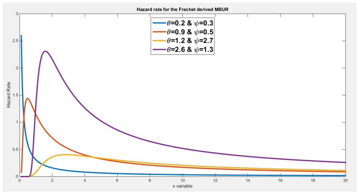
Figure 13, Figure 14 and Figure 15 show the PDF, CDF, and hazard function of the distribution at different parameter values. The distribution is highly skewed with long right tail.

Theorem 10: the quantile function can be expressed as

{(\frac{- 1}{ψ} \ln c)}^{\frac{- 1}{θ}}

Proof:

F_{X} (x) = 3 e^{- {2 ψx}^{- θ}} - 2 e^{- {3 ψx}^{- θ}}

can be rewritten as

u = 3 e^{- {2 ψx}^{- θ}} - 2 e^{- {3 ψx}^{- θ}} = 3 {(e^{- {ψx}^{- θ}})}^{2} - 2 {(e^{- {ψx}^{- θ}})}^{3}

, this third degree polynomial has the following root:

e^{- {ψx}^{- θ}} = \{- . 5 (\cos [\frac{\cos^{- 1} (1 - 2 u)}{3}] - \sqrt{3} \sin [\frac{\cos^{- 1} (1 - 2 u)}{3}]) + . 5\} = c

- {ψx}^{- θ} = \ln c \to x^{- θ} = \frac{- 1}{ψ} \ln c \to x = {(\frac{- 1}{ψ} \ln c)}^{\frac{- 1}{θ}}

Theorem 11: The r^th raw moment is given by

μ_{r}^{'} = 3 {(2 ψ)}^{\frac{- r}{θ}} Γ (1 - \frac{r}{θ}) - 2 {(3 ψ)}^{\frac{- r}{θ}} Γ (1 - \frac{r}{θ}), (1 - \frac{r}{θ}) > 0

Proof

E (x^{r}) = 6 ψθ \int_{0}^{\infty} x^{r} x^{- θ - 1} e^{- {2 ψx}^{- θ}} [1 - e^{- {ψx}^{- θ}}] dx

Let

{y = x}^{- θ} \to x = y^{\frac{- 1}{θ}} \to dx = \frac{- 1}{θ} {(y)}^{\frac{- 1}{θ} - 1} dy

= 6 ψθ \int_{0}^{\infty} {(y^{\frac{- 1}{θ}})}^{r} {(y^{\frac{- 1}{θ}})}^{- θ - 1} e^{- {2 ψ (y^{\frac{- 1}{θ}})}^{- θ}} [1 - e^{- {ψ (y^{\frac{- 1}{θ}})}^{- θ}}] (\frac{1}{θ} {(y)}^{\frac{- 1}{θ} - 1} dy)

= 6 ψ \int_{0}^{\infty} y^{\frac{- r}{θ}} e^{- 2 ψy} [1 - e^{- ψy}] dy

= 6 ψ \int_{0}^{\infty} y^{\frac{- r}{θ}} e^{- 2 ψy} dy - 6 ψ \int_{0}^{\infty} y^{\frac{- r}{θ}} e^{- 3 ψy} dy

= 6 ψ \frac{Γ (1 - \frac{r}{θ})}{{(2 ψ)}^{1 - \frac{r}{θ}}} - 6 ψ \frac{Γ (1 - \frac{r}{θ})}{{(2 ψ)}^{1 - \frac{r}{θ}}} = 3 {(2 ψ)}^{\frac{- r}{θ}} Γ (1 - \frac{r}{θ}) - 2 {(3 ψ)}^{\frac{- r}{θ}} Γ (1 - \frac{r}{θ})

Where

1 - \frac{r}{θ} > 0 \to 1 > \frac{r}{θ} \to θ > r

Theorem 12: The asymptotic limiting distribution is Frechet as (n) approaches infinity.

Proof: follow the previous steps to get the normalizing constants, then substitute in the CDF of the new distribution, raise to the power of n and evaluate the limit as n approaches infinity.

\frac{n}{n + 1} = 3 e^{- {2 ψ (b_{n})}^{- θ}} - 2 e^{- {3 ψ (b_{n})}^{- θ}} = 3 e^{- {2 ψ (b_{n})}^{- θ}} (1 - \frac{2}{3} e^{- {ψ (b_{n})}^{- θ}})

as (b_{n}) \to \infty, e^{- {ψ (b_{n})}^{- θ}} ≅ 1

F_{X} (x) = 3 e^{- {2 ψ (b_{n})}^{- θ}} (1 - \frac{2}{3}) = 3 e^{- {2 ψ (b_{n})}^{- θ}} (\frac{1}{3}) = e^{- {2 ψ (b_{n})}^{- θ}}

\frac{n}{n + 1} = e^{- {2 ψ (b_{n})}^{- θ}} \to \frac{n + 1}{n} = e^{{2 ψ (b_{n})}^{- θ}} \to \ln (1 + \frac{1}{n}) = {2 ψ (b_{n})}^{- θ} \to \frac{1}{n} = {2 ψ (b_{n})}^{- θ}

\to \frac{1}{2 ψn} = {(b_{n})}^{- θ} \to 2 ψn = {(b_{n})}^{θ} \to b_{n} = {(2 ψn)}^{\frac{1}{θ}} = let a_{n} = {(2 ψn)}^{\frac{1}{θ}}

F_{X} (x) = e^{- {2 ψ ({(2 ψn)}^{\frac{1}{θ}} x + {(2 ψn)}^{\frac{1}{θ}})}^{- θ}} = e^{- {2 ψ ({(2 ψn)}^{\frac{1}{θ}} (x + 1))}^{- θ}}

= e^{- 2 ψ {(2 ψn)}^{- 1} {(x + 1)}^{- θ}} = e^{- {(n)}^{- 1} {(x + 1)}^{- θ}}

\lim_{n \to \infty} {[F_{X} (x)]}^{n} = {[e^{- \frac{1}{n} {(x + 1)}^{- θ}}]}^{n} = e^{- n \frac{1}{n} {(x + 1)}^{- θ}} = e^{- {(x + 1)}^{- θ}}

Let us call x+1=v

\lim_{n \to \infty} {[F_{X} (x)]}^{n} = e^{- v^{- θ}}

The asymptotic limiting distribution is Frechet.

So according to the transformation applied on the MBUR, two different types of the extreme value distributions can be obtained as illustrated above, the Gumbel and the Frechet. Moreover, according to the steps, either two step or one steps, as illustrated in section 2 and 3, the Gumbel asymptotic limiting distribution can be attained.

Section 5: The asymptotic limiting distribution of the MBUR distribution is Weibull distribution

There are two approaches to prove this limit.

First approach: y follows the MBUR with the following CDF

F_{Y} (y) = 3 y^{\frac{2}{α^{2}}} - 2 y^{\frac{3}{α^{2}}}

, which can be rewritten as

F_{Y} (y) = 3 y^{\frac{2}{α^{2}}} (1 - \frac{2}{3} y^{\frac{1}{α^{2}}})

.

At the upper boundary, y = 1

F_{Y} (y) = 3 y^{\frac{2}{α^{2}}} (1 - \frac{2}{3}) = 3 y^{\frac{2}{α^{2}}} (\frac{1}{3}) = y^{\frac{2}{α^{2}}}

Multiply both sides by

(\frac{- 1}{n})

\frac{{- F}_{Y} (y)}{n} = - \frac{y^{\frac{2}{α^{2}}}}{n}

Add (1) to both sides

1 - \frac{F_{Y} (y)}{n} = 1 - \frac{y^{\frac{2}{α^{2}}}}{n}

Take the power of both sides, raised to n:

{[1 - \frac{F_{Y} (y)}{n}]}^{n} = {[1 - \frac{y^{\frac{2}{α^{2}}}}{n}]}^{n}

Take the limit of both sides

\lim_{n \to \infty} {[1 - \frac{F_{Y} (y)}{n}]}^{n} = \lim_{n \to \infty} {[1 - \frac{y^{\frac{2}{α^{2}}}}{n}]}^{n}

e^{- [F_{Y} (y)]} = e^{y^{- \frac{2}{α^{2}}}}

Second approach : As the distribution is defined on the unit interval so b_n = 1 ( upper boundary). The a_n represents the gap which scales dynamically as (1 − b_n). Let us define (t) as the distance from the [y _(n)] to upper boundary as y _(n) = 1 − t

Take the Tayler series expansion of the CDF at the boundary, y=1

F_{Y} (1) = 1, F_{Y}^{'} (1) = 0, F_{Y}^{″} (1) = \frac{- 6}{α^{4}}

F (y_{(n)}) = F_{Y} (1) + F_{Y}^{'} (1) y_{(n)} + \frac{F_{Y}^{″} (1)}{2} y_{(n)}^{2}

F (1 - t) = F_{Y} (1) + F_{Y}^{'} (1) t + \frac{F_{Y}^{″} (1)}{2} t^{2}

F (1 - t) = 1 - \frac{6}{2 α^{4}} t^{2}

Map MBUR CDF at y _(n) , expressed in Tayler series expansion, to the expected value of largest order statistics drawn from the uniform distribution

1 - \frac{1}{n + 1} = F (1 - t) = 1 - \frac{6}{2 α^{4}} t^{2}

\frac{1}{n + 1} = \frac{6}{2 α^{4}} t^{2} = \frac{3}{α^{4}} t^{2}

t^{2} = \frac{α^{4}}{3 (n + 1)} \to t = \frac{α^{2}}{\sqrt{3 (n + 1)}}

b_{n} = 1 and a_{n} = \frac{α^{2}}{\sqrt{3 (n + 1)}}

The linear transformation is

y_{(n)} = \frac{α^{2}}{\sqrt{3 (n + 1)}} y + 1

, the distance from the y_(n) to the ceiling boundary which is 1 is

t = 1 - y_{(n)} = 1 - (\frac{α^{2}}{\sqrt{3 (n + 1)}} y + 1)

.

So the distance (t) is

t = (\frac{α^{2}}{\sqrt{3 (n + 1)}} y)

, square this distance and substitute it in the Tayler series expansion

F (y_{(n)}) = F (a_{n} y + b_{n}) = 1 - (\frac{3}{α^{4}}) [\frac{α^{4}}{3 (n + 1)}] y^{2} = 1 - \frac{y^{2}}{n + 1}

\lim_{n \to \infty} {[F (y_{(n)})]}^{n} = \lim_{n \to \infty} {(1 - \frac{y^{2}}{n + 1})}^{n} = e^{- y^{2}}

The limiting distribution is Weibull, type III of extreme value distribution.

Conclusions

Median based unit Rayleigh (MBUR) is a distribution defined on the unit interval. Its asymptotic limiting behavior is The Weibull distribution, type III generalized value distribution. From this MBUR, new distributions can be derived depending on the transformation implemented on it. In two successive steps of transformation, Gumbel distribution can be obtained. First applying the negative log squared transformation on the MBUR random variable, then another negative log transformation on the new PDF derived from the first transformation. Moreover, one step transformation, by applying negative double transformation with parametrization of the variable can yield the Gumbel distribution as an asymptotic limiting distribution as n approaches infinity. Lastly, Frechet asymptotic limiting distribution is the result achieved after applying the appropriate one step transformation on the MBUR random variable as explicated in section 4. Each of these transformation gives a new distribution with different supports and properties like the PDF, CDF, hazard rate, quantile functions and r^th raw moments.

Funding

No funding resource. No funding roles in the design of the study and collection, analysis, and interpretation of data and in writing the manuscript are declared

Ethics approval and consent to participate

Not applicable.

Consent for publication

Not applicable

Availability of data and material

Not applicable. Data sharing not applicable to this article as no datasets were generated or analyzed during the current study.

Competing interests

The author declares no competing interests of any type.

Authors’ contribution

AI (Attia Iman) carried the conceptualization by formulating the goals, aims of the research article, formal analysis by applying the statistical, mathematical and computational techniques to synthesize and analyze the hypothetical data, carried the methodology by creating the model, software programming and implementation, supervision, writing, drafting, editing, preparation, and creation of the presenting work.

Acknowledgement

Not applicable

References

Attia, I. M. (2025). The new generalized odd Median Based Unit Rayleigh. Frontiers in Applied Mathematics and Statistics, 11, 1648127. [CrossRef]
Beirlant, J., Goegebeur, Y., Teugels, J., & Segers, J. (2004). Statistics of Extremes: Theory and Applications (1st ed.). Wiley. [CrossRef]
De Haan, L., & Ferreira, A. (2006). Extreme Value Theory: An Introduction. Springer New York. [CrossRef]
Fisher, R. A., & Tippett, L. H. C. (1928). Limiting forms of the frequency distribution of the largest or smallest member of a sample. Mathematical Proceedings of the Cambridge Philosophical Society, 24(2), 180–190. [CrossRef]
Haan, L. D. (1976). Sample extremes: An elementary introduction. Statistica Neerlandica, 30(4), 161–172. [CrossRef]
Kotz, S., & Nadarajah, S. (2000). Extreme Value Distributions: Theory and Applications. PUBLISHED BY IMPERIAL COLLEGE PRESS AND DISTRIBUTED BY WORLD SCIENTIFIC PUBLISHING CO. [CrossRef]
Leadbetter, M. R., Lindgren, G., & Rootzén, H. (1983). Extremes and Related Properties of Random Sequences and Processes. Springer New York. [CrossRef]
Mood, A. M., Graybill, F. A., & Boes, D. C. (1974). Introduction to the Theory of Statistics. (3rd edition). McGraw-Hill, New York.
Reiss, R.-D., & Thomas, M. (2007). Statistical Analysis of Extreme Values: With Applications to Insurance, Finance, Hydrology and Other Fields. Birkhäuser Basel. [CrossRef]
Resnick, S. I. (1971). Tail equivalence and its applications. Journal of Applied Probability, 8(1), 136–156. [CrossRef]
Resnick, S. I. (1987). Extreme Values, Regular Variation and Point Processes. Springer New York. [CrossRef]
Resnick, S. I. (2007). Heavy-Tail Phenomena: Probabilistic and Statistical Modeling. Springer New York. [CrossRef]

Figure 1. shows the PDF of the NLS-MBUR distribution. It is highly right skewed with long right tail.

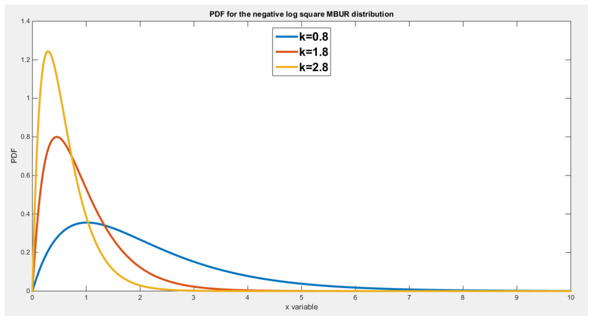
Figure 2. shows the CDF of the NLS-MBUR.

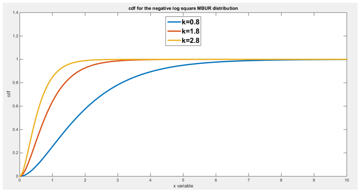
Figure 3. Hazard rate function of the NLS-MBUR distribution. It shows an increasing pattern then almost constant rate which is (k) as (x) approaches infinity.

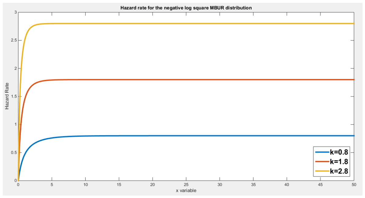
Figure 4. shows the PDF of the negative double NSL-MBUR distribution.

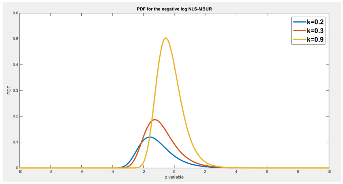
Figure 5. depicts the CDF of the negative double NSL-MBUR distribution.

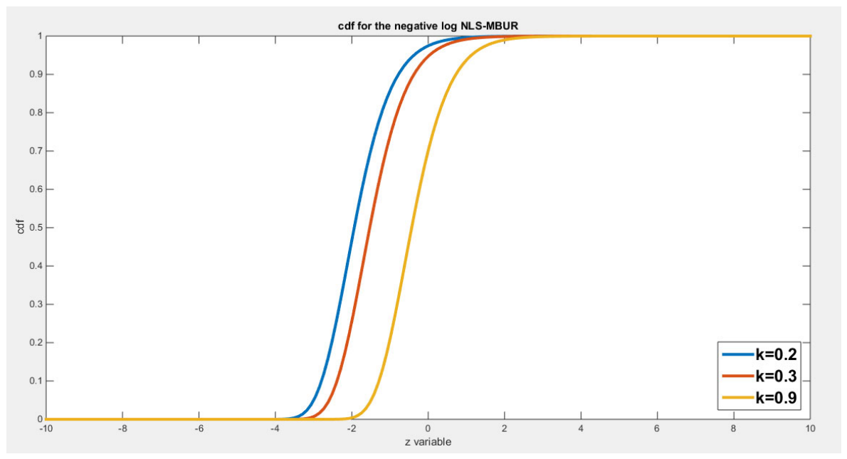
Figure 6. illustrates the Hazard rate function for the distribution. It is constant at zero then increased and drops again to zero.

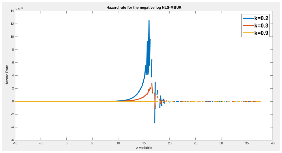
Figure 7. shows the PDF of the distribution.

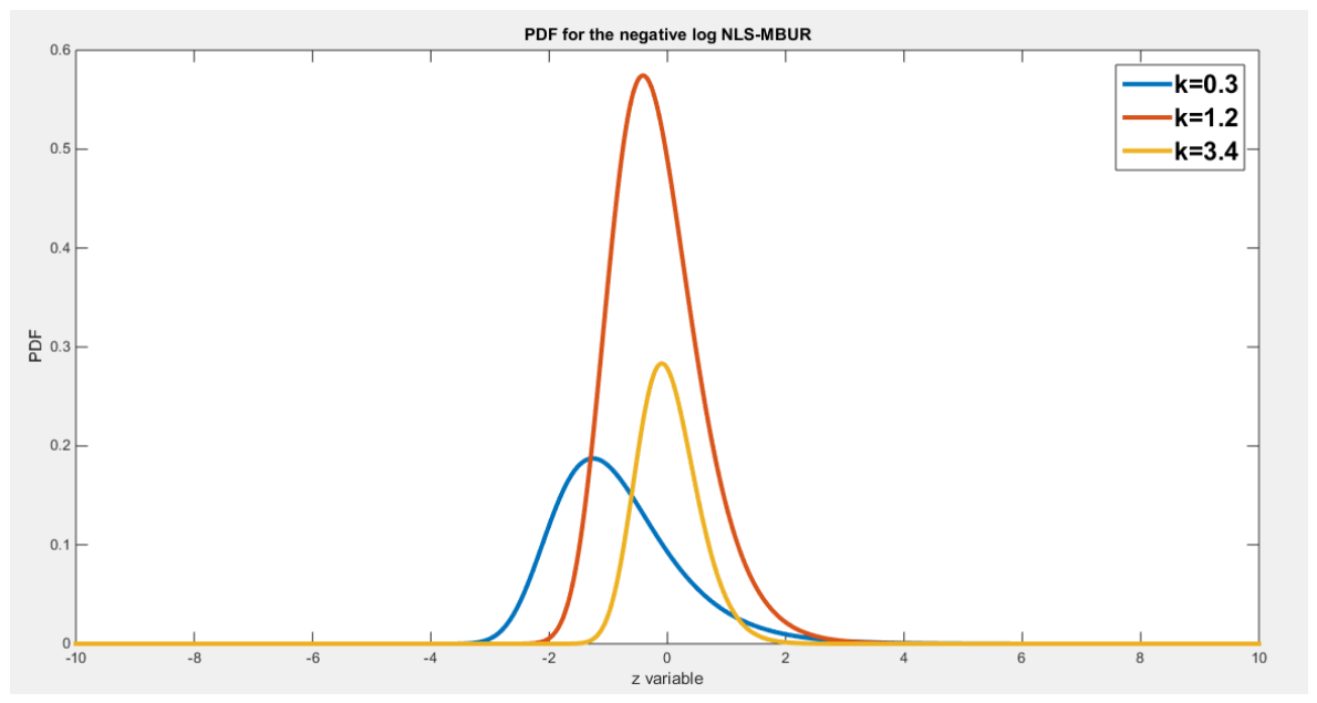
Figure 8. shows the CDF of the distribution.

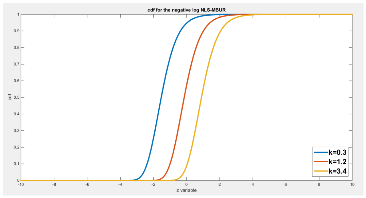
Figure 9. depict the hazard rate function of the distribution, at parameter value less than one the function initially increased to high values then decreased to zero as shown in figure 6. The same pattern is achieved for parameters greater than one, but the difference is the values at which the hazard function reaches the maximum then drop to zero. These values are higher, at parameter values less than one, than those at parameter values greater than one.

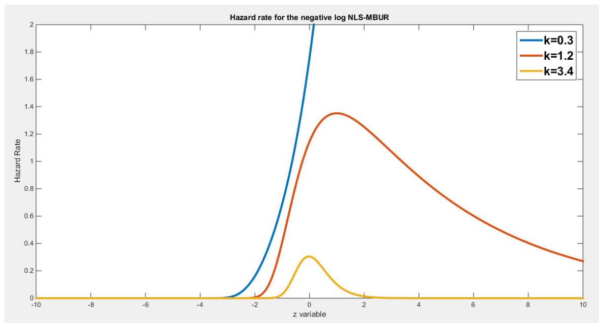
Figure 10. represents the different shapes of the PDF at different parameter values.

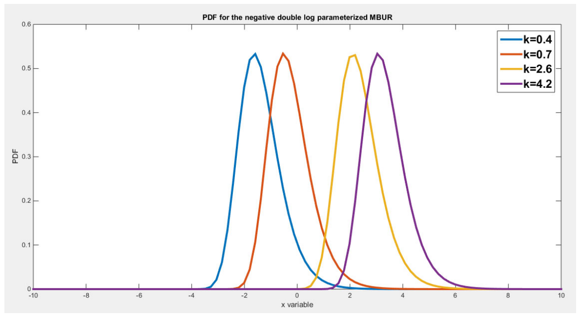
Figure 11. shows the CDF of the distribution at different parameter values.

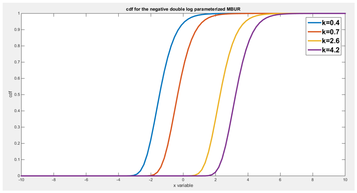
Figure 12. shows the hazard function at different parameter values. As shown in the figure the hazard initially increased from zero to attain a constant level at almost 2 then starts to drop again to zero. Before this drop it may reach some higher values than 2. This pattern of behavior is shown either at parameter values less than one or greater than one.

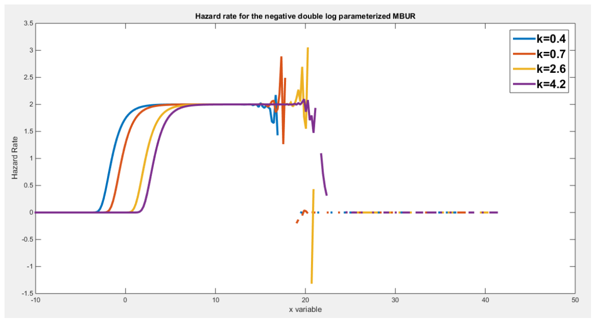
Figure 13. shows the different shapes of the PDF at different parameters values.

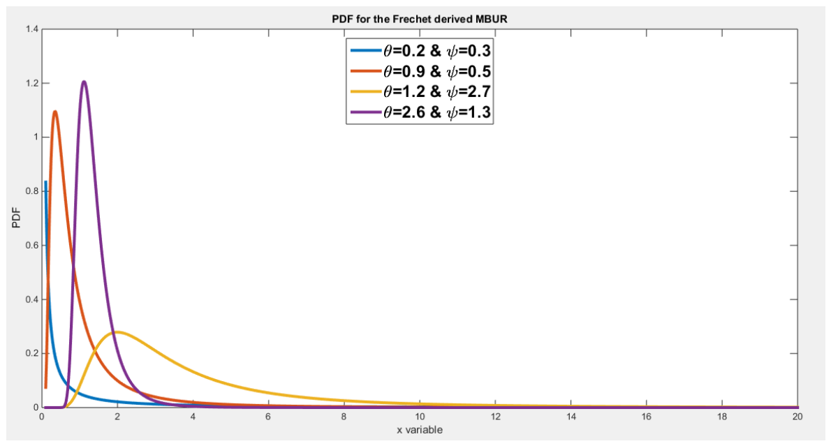
Figure 14. shows the different CDF at different parameter values.

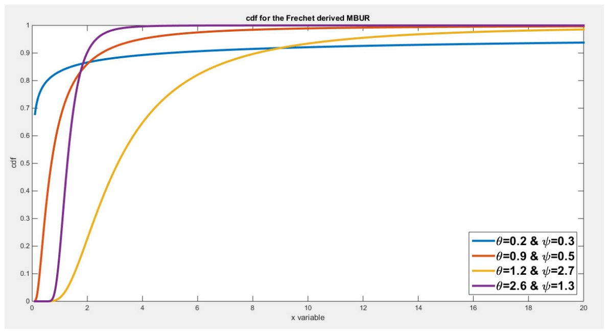
Figure 15. shows the hazard function. At parameter values less than one the hard in decreasing function. While at levels greater than one, it is increasing then decreasing.

Disclaimer/Publisher’s Note: The statements, opinions and data contained in all publications are solely those of the individual author(s) and contributor(s) and not of MDPI and/or the editor(s). MDPI and/or the editor(s) disclaim responsibility for any injury to people or property resulting from any ideas, methods, instructions or products referred to in the content.

© 2026 by the authors. Licensee MDPI, Basel, Switzerland. This article is an open access article distributed under the terms and conditions of the Creative Commons Attribution (CC BY) license (http://creativecommons.org/licenses/by/4.0/).

Copyright: This open access article is published under a Creative Commons CC BY 4.0 license, which permit the free download, distribution, and reuse, provided that the author and preprint are cited in any reuse.