

Submitted:
19 October 2026
Posted:
20 October 2026
You are already at the latest version
Abstract
There is a lack of comparative XAI evaluations for sensor-based quality monitoring (SBQM) appli-cations in the context of construction and demolition waste (CDW) management. Moreover, such studies are generally oriented towards classification architectures and tasks. To address these gaps, we compared the faithfulness, stability and localization of three common post-hoc XAI evaluation methods, namely Grad-CAM, LIME and SHAP. These post-hoc methods were implemented into a multitask-CNN, i.e. CDW-MT-CNN, containing an identical classification and regression head architecture. No single method excels on all aspects: only Grad-CAM is fast and stable enough for near-real-time monitoring (10 ms/instance) but suffers from its large receptive field limitation, impacting its faithfulness and localization. LIME and SHAP are faithful and localize well but have limited stability and their computational overhead (180–600 ms/instance) renders them unsuitable for the near-real-time application. Further research in the directions of correlation studies between explanation and predictive quality, a detailed sensitivity study of the hyperparameters for LIME and SHAP, explainability evaluations of advanced gradient-based methods that mitigate the large receptive field limitation, and a detailed per-image runtime and energy consumption study on representative recycling plant hardware would further contribute to responsible deployment of XAI in SBQM for CDW management.
Keywords:
construction and demolition waste (CDW)
; explainable artificial intelligence (XAI)
; sensor-based quality monitoring
; convolutional neural networks (CNNs)
; multitask learning
1. Introduction
Construction and demolition waste (CDW) is one of the high-impact streams with untapped potential when it comes to the transition towards a circular economy [1,2]. Even though recorded recycling rates for CDW are generally high in Europe [3], a significant share of the material is downcycled [4,5]. To an extent, this is attributed to a lack of trust in the material for high-grade applications stemming from limited data and transparency [6,7,8]. In this context, sensor-based quality monitoring (SBQM) as part of material flow characterization is emerging as a potential key enabler to fill this gap [9]. This approach utilizes (optical) sensors mounted above the material stream, usually transported on a conveyor belt, to capture (image) data of this stream with real-time recording speed that are then forwarded to a data processing and analysis pipeline. Given the high complexity of such material streams and corresponding tasks, AI-based approaches are often embedded in these processing pipelines [9]. The goal of such quality monitoring is to characterize the bulk flow, therewith providing operators, plant managers and downstream users with continuous, detailed and reliable quality information about the material being produced for recycling applications.
In a previous work, we systematically investigated the current state of SBQM for CDW processing compared to other fields and found that most research remains at a proof-of-concept laboratory scale [10]. At the same time, we found that visual image sensing paired with machine learning was a predominant technology being investigated at the time [10]. In a follow-up investigation, we therefore developed a custom, lightweight multitask-CNN architecture for the real-time monitoring of comminuted CDW in the context of full-scale mobile comminution [11]. In this architecture, a single shared backbone feeds two heads that each address a part of the particle size distribution (PSD), which is one of the main quality factors for this material stream: one head classifies the particles to their size class, whereas the other head estimates the particle’s weight.
However, in the context of increasing data transparency, a major difficulty remains. That is, most machine learning models, including the previously-used CNN architecture, are black box, where the quality and validity of individual decisions in principle cannot be inspected. At the same time, taking into account the context of practical implementation in the CDW comminution industry, several stakeholder groups would benefit from the ability to inspect why the model arrived at a given decision. For instance, plant operators require interpretable feedback to recognize drift or other anomalies in the input material stream for timely adjustment of the machine settings. Similarly, quality managers need defensible, traceable evidence that the SBQM system’s output reflects true material properties, an aspect that is also gaining importance for the development of digital material or product passports in the construction sector [12,13]. Recent advances in explainable AI (XAI) may close this gap. As such, this study compares prominent post-hoc XAI methods that extend the previously developed CNN-architecture as add-on explainability modules. This may contribute to (X)AI developments at the intersection of computer science and waste management, where practice-oriented approaches are eminent. Specifically, this study investigates and systematically compares different approaches to address the post-hoc model explainability problem in the context of SBQM of the complex CDW material stream for CNN-based multitask prediction.
1.1. Related Work
The review by Langley et al. [14] highlights the advancement from preliminary object detection towards real-time segmentation models and addresses a common problem preexisting in AI-developments for waste management applications: the simplification of sample material in order to be able to validate the developed models or systems. However, CDW is a complex, multi-material stream characterized by among other things high bulk throughput, large vibrations in the surrounding environment as well as dust, changes in illumination and presence of potential contaminants [15]. In recent years, for SBQM, investigations — including some by the authors of this work — have mainly focused on utilizing greyscale or pointcloud and RGB image data stemming from 3D-laser triangulation and RGB-(line scan) sensors, respectively [16,17,18,19]. In some of these works, preliminary implications on model explainability are considered (e.g. ref. [17]). However, to the authors’ knowledge, thus far no in-depth study on the usability and applicability of these XAI methods as well as considerations for practical implementation are available in this field. Additionally, as practical consideration, Jean-Quartier et al. argue that the sustainability impacts in terms of energy demand stemming from the computational demand are often ignored even though the choice of XAI method has a measurable effect on energy consumption [20].
In the broader field of AI, on the other hand, XAI has matured into a large field with its own surveys and taxonomies [21,22]. For instance, Dib and Capus [23] propose a three-dimensional classification of explanatory approaches along the axes of intrinsic–extrinsic, model-specific–model-agnostic and local–global to clarify the difference between interpretability and explainability. Following their definition, the intrinsic–extrinsic dimension regards the transparency of a model, i.e. explainability (the model’s decision-making) and interpretability (understanding the model’s functioning). In this context, intrinsic refers to a model’s capability of providing this information directly from its internal structure, whereas extrinsic refers to the use of external (i.e. post-hoc) techniques to make this information available. The model-specific–model-agnostic dimension regards the differentiation between approaches implementable for specific architectures only and approaches that can be used for any type of model whatsoever. Lastly, the local–global dimension separates approaches that justify individual predictions (local) from those that also by definition analyze the model’s internal functioning (global).
An important consensus from recent XAI-literature is that explanations should not be judged by visual plausibility, as a plausible-looking heatmap can nonetheless be unfaithful. Instead, several metrics that regard different aspects of model explanations have been developed. Faithfulness can for instance be measured by computing perturbation-based curves. That is, deletion and insertion procedures progressively mask or reveal important regions and record the corresponding change in model output to quantify the faithfulness of an explanation [24,25]. That is, it measures the accuracy of the attribution map reflecting the true importance of input features. Another metric is explanation stability, the quantification of similarity for semantically equivalent inputs through similarity metric computations under controlled perturbations such as Gaussian noise [26]. When assessing explainability methods on the basis of stability, according to the study by Alvarez-Melis and Jaakkola [26], several popular methods are deemed fragile and overly sensitive to perturbations. Similarly important is the localization metric, which quantifies the degree of attributions that concentrate on the object of interest. For this, rank-based overlap metrics used against a reference region are generally applied [27] to minimize sensitivity to region size [28].
In the work by Skliarov et al. [29], commonly-used attribution map explainability methods are compared in terms of fidelity, identity, separability and computational time, indicating the variety of aspects that can be measured when assessing explainability methods. More specifically, they compared local interpretable model-agnostic explanations (LIME) [30], Shapley additive explanations (SHAP) [31], and a set of gradient-based class activation mapping methods (e.g. Grad-CAM [32]) and found that no single method excels across all metrics. The suggestion that method applicability and usability is task- and metric-dependent is further indicated in the work by Nazim et al. [33], where the joint implementation of SHAP, LIME and Grad-CAM is investigated for malware-image classification. These studies however focus solely on classification models, whereas a comparison for regression architectures remains largely unexplored. Correspondingly, Letzgus et al. [34] provide methodological foundations of XAI for regression and show that regression explanations raise distinct challenges around the choice of reference baseline, the sign of attributions and the additivity of contributions across spatial regions. For instance, the calculation procedures of many evaluation metrics are originally based on classification scores, which makes transferring them to a regression head non-trivial. For instance, many calculations of explainability metrics are originally based on classification scores, which makes transferring them to regression heads a non-trivial procedure.
1.2. Aims and Research Questions
Several research gaps can be extracted from the related work. First, we identified that comparative XAI evaluation studies are oriented towards classification architectures and tasks, generally ignoring the regression counterpart. Second, no comparative XAI evaluation for SBQM applications in the context of waste management could be identified in the literature. In line with this, the third research gap is the limited addressing of implications for stakeholders in practice. In the context of SBQM, this particularly regards implications on the suitability of XAI methods to support human oversight of the monitoring system and plant constraints such as latency or energy limits. In this work, we address these gaps for three of the most common post-hoc XAI methods — Grad-CAM, SHAP and LIME — by answering the following two research questions:
RQ1: How do the three post-hoc methods Grad-CAM, LIME and SHAP compare in terms of faithfulness, stability and localization for both regression and classification when applied to a multitask-CNN developed for SBQM of CDW material streams?
RQ2: What practical trade-offs does each method impose under the industrial constraints of real-time SBQM of CDW material streams?
2. Materials and Methods
2.1. Data Set
The data utilized in this study stems from a data set used in our previous work [11] and contains 1470 comminuted CDW particles with size classes ranging from 4 to 63 mm and particle weights ranging from several milligrams to around 150 g. More details on the sampling and classification procedure of this material as well as the laboratory analysis and data acquisition can be found in our previous publication [11].
In the data set, each particle is individually presented against a black background. These images are stored as 224 by 224 pixel PNG files and are accompanied with labels containing the particle weight and size class ground truth. As such, each instance yields four elements that are used in this work: the image tensor, an integer size-fraction class that can be mapped to common class naming terminology, a particle weight floating point label, and a binary particle mask derived from the image itself. Using stratified random sampling on the particle size class, 296 samples were saved separately to be used as test set, containing an imbalance ratio of around 2.5:1. An overview of the distribution of the data set is provided in Table 1.
2.2. The CDW-MT-CNN Model
In our previous publication [11], we introduced a multitask-CNN architecture that is able to simultaneously predict the particle size class and weight of a segmented particle. In this work, we further optimized this architecture to better handle spatial information even in the deeper layers for either head and have slightly better performance being trained and tested on the exact same data sets: 82.3% global accuracy (particle size classification) and 12.8 g RMSE (particle weight regression), compared to the previously achieved 81.7 % global accuracy and 14.3 g RMSE. Additionally, we redesigned the architecture in such a way that this improved performance is achieved for heads with identical architecture, except for the final layer where the output is provided, such that a comparison is based only on the differences related to the distinct tasks. This forms the basis for the experiments conducted in this work: the optimized architecture is elaborated with Grad-CAM, LIME and SHAP implementations to perform a multi-level comparison of these common post-hoc XAI methods (see Figure 1). More details on the experimental procedure are provided in the following sections.
2.3. XAI Methods
2.3.1. Grad-CAM
Grad-CAM, introduced by Selvaraju et al. [32], is a gradient-based, model-specific, local explanation method. The aim of this method is to identify which spatial regions of an input image most strongly support a chosen model output by exploiting the gradients that flow into the convolutional feature maps of the neural network. The activation of deep convolutional layers can then be projected back onto the image as a heatmap of evidence due to the layers’ spatial correspondence retention characteristic.
Typically, feature maps of the last convolutional layer are extracted. For each feature map, a weight equal to the average gradient is computed and then combined as a weighted sum. This weighted-sum representation of all feature maps is then rectified to only retain regions with a positive contribution to the output and upsampled to the input resolution using bilinear interpolation. A single forward and backward pass finally produce the explanation.
This approach makes Grad-CAM an efficient method that yields smooth and interpretable attribution or activation maps. However, the activation region can spill beyond the object’s boundary due to the spatial resolution of the explanation being tied to the resolution of corresponding the deep feature map, which may also cause inaccuracies in case the receptive field is larger than the target object [35]. Additionally, the implementation of Grad-CAM is only possible when access to the network’s internal feature maps and gradients is available. The method is also originally designed for classification, meaning that for explaining a continuous regression target a suitable scalar score must be selected.
2.3.2. LIME
The LIME method was introduced by Ribeiro et al. [30] and is a perturbation-based, model-agnostic, local explanation method that approximates the behavior of a complex model in the immediate neighborhood of a single prediction on the basis of a surrogate model. The coefficients of this surrogate model serve as the explanation, which means that no assumptions about the internal structure of the model need to be made. For image inputs specifically, LIME segments the image into superpixels and generates perturbed versions of the image by deactivating certain superpixels. The model is then queried on each image perturbation to fit a sparse weighted linear model to the resulting input-output pairs, weighted by the sample’s proximity to the original image. To form the attribution map, each superpixel is assigned a certain importance.
Contrary to Grad-CAM, LIME can be used on models where the internal architecture is not accessible, as it requires only to query the model’s outputs. Additionally, the surrogate approach is intuitive and the spatial resolution can be tuned through the choice of superpixel segmentation. However, this also means that a large number of model evaluations is needed, making it less efficient. Additionally, the fidelity of the surrogate is guaranteed only locally and explanations are sensitive to the choice of superpixel segmentation as well as the sampling procedure.
2.3.3. SHAP
The fundamental concept of SHAP, introduced by Lundberg and Lee [31] is a game-theoretic, model-agnostic, local explanation approach: each input feature is treated as a player, the prediction as the payoff and the explanation is represented by the average marginal contribution across all possible coalitions of features (i.e. the Shapley value). As such, the feature contributions sum to the difference between prediction and reference baseline. For image inputs, a kernel-based variation is applied on superpixels due to the high computational demand of Shapley estimations. That is, coalitions of present and absent superpixels are sampled, after which the model is evaluated on corresponding masked images. Similar to LIME, a weighted linear regression recovers the Shapley values and allows to form the attribution map.
SHAP has a strong theoretical foundation with properties of symmetry and additivity as well as the ability to assign signed contributions to corresponding features. However, the approach is computationally intensive because of the need to evaluating the model over many coalitions. Additionally, the quality of the estimate is sensitive to the number and kind of coalitions being evaluated.
2.4. Evaluation Metrics
The metrics of focus in this work were chosen to be consistent with recent XAI-evaluation literature and reproducible through established toolkits, such as Quantus [36]. As such, the metrics of interest are faithfulness [24], stability [26] and localization [28].
Faithfulness is evaluated by deletion and insertion curves, which are computed by progressively removing or revealing pixels against a reference baseline, respectively. This is quantified by the area under curve (AUC), where a low deletion AUC and a high insertion AUC indicate that the explanation as correctly identified influential regions. For Grad-CAM the dense, almost tie-free ordering allows the image to be peeled pixel by pixel outward from the most strongly activating region. For LIME and SHAP the ties among the pixels of a superpixel mean that deletion proceeds one superpixel at a time: with only about thirty importance levels the metric can express no ranking finer than the segmentation, so the AUC is decided by which segments are influential rather than by any sub-segment detail.
To quantify stability, three main metrics were computed for the attribution map of a clean image and the attribution map of a perturbed copy and considered for both the global map (i.e. entire image) and the most important pixels (i.e. top-K): the Spearman () and Kendall () rank correlation, and Pearson linear correlation (). Where and measure if the original ranking matches the perturbation ranking with different sensitivities, measures the linear relationship on important pixels. So, and provide information on the rank-based and on the magnitude-based stability [26,37,38,39]. Images were perturbed with the aim of retaining realistic images while applying visible adjustments. To do so, three types of adjustments were applied: 1) dimming of the illumination (multiplicative factor 0.85), 2) adding a small spatial jitter (2-pixel cyclic shift), and 3) adding additive sensor noise (additive Gaussian with of 0.02).
For localization, again, two statistics are utilized. The relevance rank accuracy (RRA) and the intersection-over-union (IoU) were computed to identify what fraction of the highest-ranked attribution relevances falls inside the particle mask (i.e. ground truth) and to quantify the top-attributed region, respectively. To minimize bias by the relative size of the particle, both metrics are calculated with a threshold K — similar to the stability calculations, which is tied to the mask size, following Arras et al. [28]. For Grad-CAM, the continuous field yields a genuine pixel ranking, so the top-K pixels are the single hottest contiguous region and localization becomes a question of how well that region fits inside the particle. For LIME and SHAP, the attribution is constant within each superpixel, so taking the top-K pixels amounts to selecting whole superpixels in order of their value until K pixels have been gathered. The RRA of a Shapley map is therefore not a smooth overlap but a test of whether the highest-valued superpixels lie inside the particle, and because the simple linear iterative clustering algorithm (SLIC) segments are boundary-aligned, the metric rewards a method that places its largest Shapley mass on particle segments and penalizes one that spends importance on background segments in proportion to their area. This is the way in which a Shapley value is evaluated with respect to localization, namely through the placement, over boundary-aligned segments, of its largest contributions rather than through the fit of a continuous field.
Given the paired and repeated characteristic of the comparisons, statistical significance of the results is assessed using Holm-corrected two-sided Wilcoxon signed-rank tests [40] on each pair for each head and metric and bootstrapping to quantify the uncertainty in the median differences in the form of confidence intervals. So, with this test it is investigated whether the difference of the pairwise comparisons is statistically significant. Note that this does not provide information on the effect magnitude, i.e. the size of the difference, which may still be small. Additionally, the pointwise bootstrap confidence intervals are included as complementary estimates of the median paired difference, but are not directly invertible into the Wilcoxon test results. These confidence intervals were calculated using 10000 resamples of matched instances drawn with replacement.
2.5. Experiments
The settings reported here were set once and applied uniformly so that differences between methods cannot be attributed to differences in tuning. They can be categorized into four groups: 1) the explanation targets, 2) the perturbation and surrogate parameters of the methods, 3) the parameters of the evaluation metrics, and 4) the parameters of the robustness and sensitivity analyses. The optimized CDW-MT-CNN model architecture with identical heads (see Section 2.2), was used for all experiments. A graphical representation of the model can be found in Figure 1.
The explanation target refers to the CNN model’s own prediction. The explained scalar represents the score of the predicted particle size class for the classification head and the score of the predicted particle weight for the regression head, respectively. As the regression output is bounded to the physically meaningful weight range by constraining the activation, attributions were computed against the pre-activation regression score of the model, which is in line with the recommendation of Letzgus et al. [34]. This avoids distorting the gradients and therewith marginal contributions. As indicated in Figure 1, Grad-CAM is attached to the final convolutional layer of either head.
LIME and SHAP operate on a superpixel segmentation produced by the SLIC algorithm, producing a target of thirty segments to balance explanation quality against latency. With LIME, the linear surrogate was fitted using one hundred and fifty perturbed samples. Given the higher computational demands, for SHAP, only sixty coalition samples were used to estimate Shapley values, but the computations utilize the same superpixels as for LIME.
The deletion and insertion curves were computed in twenty steps, removing or revealing equal fractions of the ranked pixels at each sequence. To maximize out-of-distribution (OOD) artifacts, the reference baseline against which pixels were deleted is a set of black pixels as opposed to mean or blurred fills. Since a constant canvas may introduce spurious evidence especially when gradually introducing the pixels during insertion, for the insertion AUC calculations a Gaussian-blurred fill was used instead. This use of perturbation is in line with ref. [24]. For additional validation, however, the mean fill was analyzed, given OOD behaviour that sits between the blurred and black approach. Additionally, for the regression faithfulness evaluation, the curves were min-max normalized to allow comparison with the classification AUCs without distorting the the original distribution pattern.
Stability was evaluated on the basis of three controlled perturbations chosen to mimic realistic acquisition variation rather than adversarial worst cases: a multiplicative dimming of the image to eighty-five per cent of its intensity to emulate lamp drift or dust on the optics, a two-pixel cyclic spatial shift to emulate timing jitter in the line-scan acquisition of the SBQM, and additive Gaussian noise with a standard deviation of 0.02 of the unit intensity range to emulate sensor noise. Each perturbation was applied independently and the attribution map of the perturbed image was compared with that of the original image.
For localization, the particle mask was obtained by thresholding the summed color channels at a small positive value. Both the IoU and the RRA use a number of top-ranked pixels equal to the number of pixels in that mask, so that the metric is comparable across particles of very different sizes.
To test whether the conclusions are an artifact of the naturally imbalanced class distribution, the entire evaluation was repeated under three resampling regimes, namely the original distribution, a balanced distribution with equal representation across the retained fractions, and a left-skewed distribution that over-weights the larger fractions by downsampling the smaller half, so that any regime-dependence of the method ranking would be exposed. Finally, the analysis was run under an explicit per-image latency budget on the order of two minutes, consistent with the empirical upper bound for near-real-time operator feedback in the context of SBQM for CDW processing. This assumption is based on expert discussions that took place during the KIMBA project (C. Varli, personal communication, December 5, 2023) Consequently, the measured run times of the three methods are reported against this latency budget.
3. Results
3.1. Comparability of the Attribution Maps
In Figure 2, the attribution maps for each method on a subset of four particles for classification and regression are presented, respectively. Three observations stand out. The first regards particle size. For the smallest particles, the Grad-CAM activation region is larger than the particle itself and is often displaced from it, spilling into the surrounding background, whereas for the largest particles the activation region covers parts of the particle and can still bleed beyond its contour.
The second observation regards the difference between the methods within a single head. Grad-CAM yields a single smooth, contiguous activation region, which is a direct consequence of its derivation from a low-resolution convolutional feature map. LIME and SHAP instead partition the particle into superpixels and assign each a separate importance, so their maps are piecewise-constant and considerably more fragmented. In the examples, the two often differ in terms of superpixel importance. This is expected given that one fits a local linear surrogate and the other estimates Shapley values from a limited sample of coalitions. The fragmentation of the perturbation-based maps is not in itself a defect, but it does suggest that their apparent precision is partly an artifact of the superpixel grid rather than evidence of finer model reasoning. When comparing all three methods on the classification head, except for the second-largest particle, where SHAP and Grad-CAM assign the same area as most important, the three methods assign different areas with the highest attribution importance. This is different for the regression head, where LIME and SHAP have similar attributions for most of the important regions and Grad-CAM assigns importance to a similar area for the second-smallest (i.e. second row) particle.
Lastly, for all three methods, the attribution maps differ visibly between the two heads for the same particle, which indicates the intended different inference behaviour of the heads despite having an identical architecture as described in Section 2.2.
3.2. Explanation Faithfulness
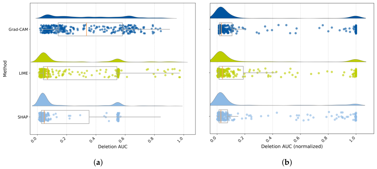
In Figure 3, the AUC distributions for the deletion curves of the classification and regression head are presented for each of the three methods. On the classification head (see Figure 3a), Grad-CAM is the least faithful method, with a median deletion area of around 0.18 — for the deletion AUC, a lower value means higher faithfulness. SHAP is most faithful, with a median deletion AUC of 0.04. The superiority of SHAP in terms of the deletion-AUC is strengthened by the low spread of its distribution, indicating high consistency over the instances. Even though LIME has a low median deletion AUC (0.05), it has the farthest outliers but with clear clusters of instances at around 0.05 and 0.55, leading to an interquartile range (IQR) that is smaller than Grad-CAM’s. For the regression head, the results are slightly different: SHAP is still most faithful with a normalized deletion AUC of 0.023 and with the lowest variance among instances. Grad-CAM now has a smaller IQR compared to LIME and a slightly lower AUC: 0.025 compared to 0.026. Additional validation using the mean perturbation baseline indicates a similar but amplified pattern. These results are documented in Appendix Figure A1.
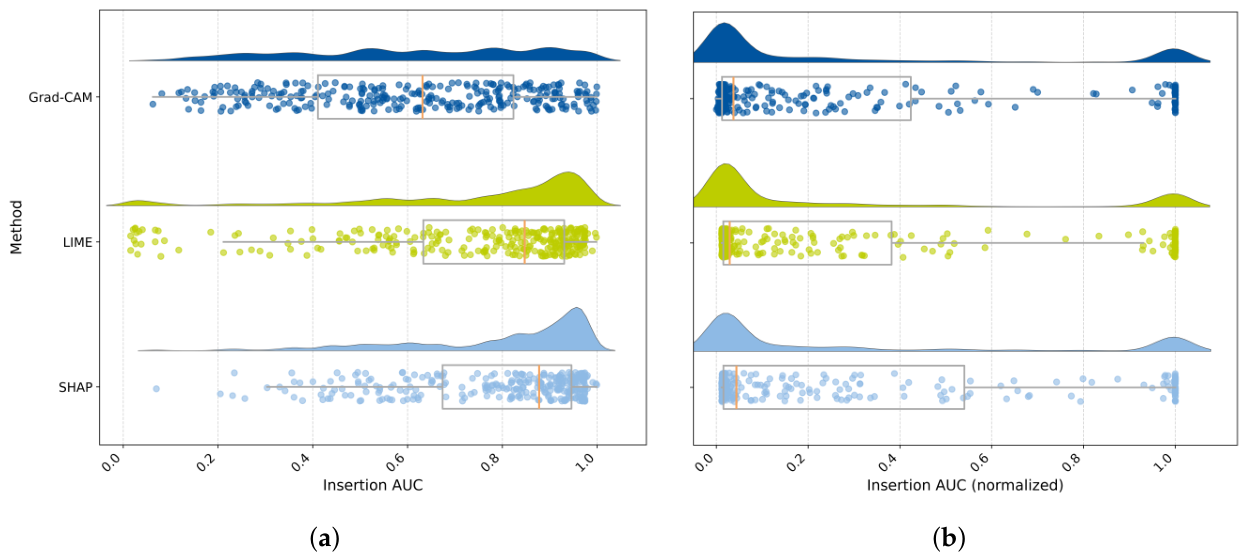
A different trend can be observed for the insertion AUC distributions (see Figure 4) for the classification head. The median insertion AUC is highest for LIME with 0.84 and lowest for Grad-CAM with 0.83, indicating that all three methods have approximately similar results. Interestingly, Grad-CAM has the smallest IQR and a slightly smaller range compared to the other two. On the regression head, all three methods have again similar performance: the normalized median insertion AUCs lie between 0.04 (SHAP) and 0.06 (LIME), and all three models have large variance and IQRs as well as clusters of instances around 0.02 and 1.00. All three median AUC values on the regression head are however low given that insertion AUCs have an ideal value of 1.0. Here, too, validation using mean perturbation provides largely the same rankings and value ranges, with the following exception: validation of the classification insertion AUC indicates SHAP as slightly superior and amplifies the limited faithfulness of Grad-CAM (see Appendix Figure A2).
The large difference between the classification and regression head results indicates the influence of the explanandum on faithfulness. For the current comparison, this may be due to the weight prediction score varying more smoothly and monotonically with the spatial extent and intensity of the particle compared to the classification score. This would translate directly into changes in the output when they are deleted or inserted, being more abrupt for the classification head compared to the regression counterpart.
3.3. Stability Under Realistic Perturbations
Figure 5 presents the median result of each stability evaluation metric for every combination of head, method and perturbation. Each method has high stability in terms of global Pearson and Spearman correlations, with the lowest value (i.e. 0.87) for SHAP on the regression head under noise perturbation. When taking into account the top-K pixels only, high stability remains for Grad-CAM with the median , and always between 0.93 and 1.00 on either head. For SHAP and LIME, the stability degrades in this perspective. Even though remains high on most occasions, with LIME on the regression head as sole exception, and are generally below 0.8 for SHAP and below 0.4 for LIME. Grad-CAMs overall stability is in line with the method’s design, which aggregates entire feature maps weighted by gradients and renders it insensitive to this kind of perturbations.
The low rank-based stability for LIME and SHAP may be caused by a reshuffling of the superpixels’ importance as a consequence of the perturbation. That remains high in general indicates that the overall importance itself remains stable. For an analyst who reads these maps to decide which region of a particle drove a prediction, the rank-based instability in the ranking is the property that matters most in practice, because it is the top-ranked regions that are generally acted upon. The fragility of perturbation-based explanations under input corruption is a phenomenon documented by Alvarez-Melis and Jaakkola [26], and the present results extend that observation to the domain of SBQM of CDW and to both heads of the CDW-MT-CNN model.
3.4. Localization
The RRA and IoU distributions, calculated against the particle mask to evaluate whether attributions concentrate on the particle itself rather than on the background, are presented in Table 2. On both heads, SHAP localizes best, with a median RRA of 0.36 and 0.35 for the classification and regression head, respectively. The result for LIME is also consistent across both heads, with median RRA-values of 0.27 and 0.24, respectively. For the IoU, a similar trend can be distinguished: LIME’s result is stable around 0.15 and SHAP has the best IoU with 0.22 for both heads. For Grad-CAM, all median values are 0.00, which corresponds with the method’s limitations described by [35], namely the assumption of spatial correspondence between features and input, which is not given for the model at hand, where the large receptive field may lead to unpreserved information, creating inaccurate explanations.
In addition, localization is also investigated per particle size class. This is done by plotting the RRA and IoU against particle size class, which results are presented in Figure 6. Localization is poor for the smallest particles, with the RRA and IoU both close to zero, and improves markedly with particle size, reaching values in the region of 0.6 to 0.9 for the largest fractions. This indicates that, for a tiny particle occupying a handful of central pixels, spillovers of attribution are more likely (see also Figure 2 and Figure 2). For a large particle, which occupies a large share of the frame, almost any attribution will land on the particle. This particle-size confound is an important caveat on the localization results and requires that aggregate localization numbers must be read in the light of the size distribution rather than as method constant.
3.5. Robustness and Statistical Significance
To assess the robustness of the results, each evaluation was repeated under three resampling regimes as described in Section 2.5. The results of this robustness test are presented in Table 3. The relative ordering of the XAI methods remains largely stable across the three regimes. For Grad-CAM, the highest fluctuations occur for the deletion AUC under the left-skewed regime on the classification head and the insertion AUC on the regression head. The stability result () however remains unchanged and desirably high. For LIME and SHAP, the deletion and insertion AUC results on both heads are stable, but fluctuations can be seen for the localization (RRA) and the stability results.
Additionally, to establish that the differences described in Section 3.2 to Section 3.4 are systematic rather than incidental, the methods were compared against each other using a paired, repeated-measures significance test, as described in Section 2.5. Since respectively three and six of the values for SHAP on the classification and regression head were undefined, these NaN-values were imputed with their medians to ensure the significance test and bootstrapping could be computed while retaining these observations under an explicit convention. To validate this approach, the results were compared to the results of leaving such pairs out completely, which provides nearly identical values. Figure 7 summarizes the outcome of the pairwise Holm-corrected Wilcoxon tests for each head. A more exhaustive presentation of the results is presented in Appendix Table A1 and includes the corrected p-values as well as the bootstrap lower and upper bounds for the 95% confidence interval. For the classification head, the insertion AUC comparison of LIME and SHAP is not statistically significant and the comparison of Grad-CAM and LIME is statistically significant at the 99% level (pHolm < 0.01). Additionally, the localization (RRA) comparison between LIME and SHAP is significant on the 99% level. Statistical significance on the 99.9% level is achieved for all other comparisons. For the regression head, with the exception of the deletion AUC of Grad-CAM and LIME, which difference is not statistically significant, the other comparison results are significant on the 99.9% level.
3.6. Computational Cost and Practical Trade-Offs
For the computational cost and practical trade-offs, the speed (i.e. time to explain a single input) and the structural properties influencing output resolution and model access of each method were analyzed. Grad-CAM is the fastest by a wide margin, because a single forward and backward pass through the network suffice to produce an explanation even within a strict real-time budget. This occurs in 10 ms on average. LIME is substantially slower with around 600 ms, because the current configuration uses one hundred and fifty forward passes through the model to fit its surrogate. This equals 4 ms per pass. SHAP is slightly faster per unit of information (i.e. 3 ms per pass), but still requires evaluating the model over many — in this case 60 — coalitions. For 60 passes, the average explanation speed is 180 ms. This ordering is in line with the analysis by Jean-Quartier et al. [20], where perturbation- and Shapley-based explanation methods have higher computational demands and consume more energy, compared to gradient-based ones. The order of 10 ms per input instance is considered suitable for near-real-time SBQM of CDW, where a single recorded images may contain hundreds to several thousands of segmentable particles. With a two-minute interval, it would mean around 12000 instances could be explained, whereas SHAP and LIME would only be able to explain several hundred instances.
Beyond explanation speed, two structural trade-offs are considered important for deployment. The first is output resolution. Grad-CAM produces a smooth, low-resolution heat map whose coarseness is intrinsic to its derivation from a deep feature map, whereas LIME and SHAP produce superpixel-level maps whose resolution is set by the segmentation and can in principle be made finer at additional computational cost. For the purpose of communicating to an operator which part of a particle drove a prediction, the coarse Grad-CAM map is usually sufficient if it provides a correct explanation without suffering from limitations related to large receptive fields. Where a finer spatial attribution is needed, the perturbation-based methods offer a tunable, if expensive, alternative. The second is model access. Grad-CAM is model-specific and requires access to the internal feature maps and gradients of the model, which is available here but would not be in a setting where the model is exposed only as a black-box service. LIME and SHAP are model-agnostic and require only the ability to query the model’s outputs, which makes them the only viable option when the internal model structure is inaccessible. An overview of the comparison is presented in Figure 8.
3.7. Limitations and Future Work
In this work, every method was run at fixed settings against the same instances and evaluated through a set of metrics implemented using established definitions. This allows for a systematic comparison between methods. Additionally, the significance of these comparisons was analyzed through Wilcoxon paired significance tests with Holm correction for multiple-comparison and robustness-tested against three class-distribution regimes. The dual-head design of the utilized CDW-MT-CNN is considered a strength in this study, as it isolates the effect of the explanandum while holding the model and the data fixed, thus enabling interpreting head-dependence as a genuine effect rather than a confound.
Nonetheless, several limitations remain. First, less well-known alternatives to Grad-CAM such as Score-CAM that may overcome some of the known limitations by Grad-CAM are not included in the present comparison. The reason for the initial decision to focus on Grad-CAM, LIME and SHAP only is that they are some of the most well-known and commonly used methods. Second, The CDW-MT-CNN model’s performance is not exhaustively analyzed in relation to the explanation-performance metric results. Third, the perturbation magnitudes, superpixel granularity, and sample budgets were fixed at single reasonable values rather than varied, so the sensitivity of the perturbation-based methods to their own hyper-parameters, a known concern for LIME in particular, was not exhaustively characterized.
Several lines of further work follow naturally from the limitations. The most immediate is to pair the explanation-performance analysis with a direct assessment of predictive performance: because ground-truth labels exist for both heads and the model’s predictive performance has already been characterized, a natural next step is to examine whether explanation faithfulness correlates with prediction error, so that explanation quality and predictive quality can be assessed together rather than separately. A second line is to characterize the sensitivity of the perturbation-based methods to their own hyperparameters by adjusting the superpixel granularity, the sample budgets, and the perturbation magnitudes, which would test whether LIME’s and SHAP’s weaknesses here are intrinsic or merely a consequence of the single operating point chosen under the latency budget. This would also allow a more elaborate assessment of explanation speed in consideration of the minimum needed number of passes to require a high-quality and valid explanation for LIME and SHAP. A third line is to broaden the method set to include gradient variants such as Score-CAM and Integrated Gradients and faithfulness controls such as fully retrained-removal benchmarks, which would situate the present three methods within a wider field while retaining the dual-head, domain-specific framing that is this study’s distinctive contribution. A fourth line is to record absolute per-image runtimes and energy consumption on representative ruggedized hardware used in waste recycling plants, turning the relative speed ordering reported here into the latency and energy quantification that a deployment decision ultimately requires.
4. Conclusions
Currently, comparative XAI evaluation studies are oriented towards classification architectures and tasks. Furthermore, there is a lack of comparative XAI evaluations for SBQM applications in the context of (CDW) waste management and, accordingly, implications for stakeholders in practice remain underaddressed. In this work, we therefore compared three post-hoc XAI evaluation methods — Grad-CAM, LIME and SHAP — in terms of faithfulness, stability and localization when applied to an optimized version of our previously-developed multitask-CNN (i.e. CDW-MT-CNN) architecture, containing a classification and regression head.
We found that no single method excels on all considered aspects of XAI, that is faithfulness, stability and localization and that the functioning of the method determines in part the applicability for practical implementation in SBQM. More specifically, Grad-CAM’s attribution maps are highly stable, both in terms of rank and magnitude which renders the method useful even in rough SBQM conditions, e.g. where illumination changes throughout the day, but the method has limited faithfulness and poor localization compared to SHAP and LIME, likely stemming from its limitation regarding large receptive fields. From a practical context, Grad-CAM’s high computational efficiency is beneficial for live monitoring, but the required access to the internal model architecture may pose limitations for its implementation. SHAP and LIME, on the other hand, do not require access to the internal architecture, are more faithful and have better localization performance. The stability is however low due to superpixel shifts and the computational efforts are higher given the required number of iterations. This renders both methods less likely to be of practical use for live implementation, but offline implementation provides explanations that are more accurate than Grad-CAM. The significance testing and the regime-robustness analysis together establish that the differences are mostly systematic rather than incidental and are not artifacts of the class balance.
By grounding the conclusions in faithfulness, stability, and localization metrics, in appropriate significance testing, and in the operational reality of the CDW recycling industry, the work offers new insights into XAI for a dual-head classification-regression multitask architecture from a domain-specific point of view and aims to contribute to the responsible deployment of XAI in sensor-based quality monitoring.
Author Contributions
Conceptualization, L.G.; methodology, L.G. and S.K.; software, L.G. and S.K.; validation, L.G. and S.K.; formal analysis, L.G. and S.K.; investigation, L.G. and S.K.; resources, L.G.; data curation, L.G.; writing—original draft preparation, L.G. and S.K.; writing—review and editing, L.G., S.K. and L.A.; visualization, L.G. and S.K.; supervision, L.G. and L.A.; project administration, L.G.; funding acquisition, –. All authors have read and agreed to the published version of the manuscript.
Funding
Parts of this work were funded by the German Federal Ministry of Education and Research (BMBF), now the German Federal Ministry of Research, Technology and Space (BMFTR), within the program "Digital GreenTech" under the project KIMBA (grant no. 2WDG1693D). Open access funding was provided by the RWTH Aachen University Open Access Publication Fund. The responsibility for the content of this publication lies with the authors.
Data Availability Statement
The datasets presented in this article are not readily available because the data are part of an ongoing study. Requests to access the datasets should be directed to the corresponding author.
Acknowledgments
Parts of this study were undertaken as a collaborative master thesis project between the Department of Anthropogenic Material Cycles at RWTH Aachen University, Germany, and the Faculty of Science at Utrecht University, The Netherlands. The authors would like to extend their appreciation to Prof. dr. Remco Veltkamp (Affiliation: Utrecht University, Faculty of Science) for his oversight and support of Sathya Santhoshi Koka during the master’s thesis and to Daan Kolkman (Affiliation: Utrecht University, Faculty of Science) for the collaboration opportunity.
Conflicts of Interest
The authors declare no conflicts of interest.
Abbreviations
The following abbreviations are used in this manuscript:
| 3D | Three-dimensional |
| AI | Artificial intelligence |
| AUC | Area under curve |
| CDW | Construction and demolition waste |
| CDW-MT-CNN | Construction and demolition waste |
| multitask-convolutional neural network | |
| CNN | Convolutional neural network |
| Grad-CAM | Gradient-weighted class activation mapping |
| IoU | Intersection-over-union |
| IQR | Interquartile range |
| LIME | Local interpretable model-agnostic explanations |
| NaN | Not a number |
| OOD | Out-of-distribution |
| PNG | Portable Network Graphics |
| PSD | Particle size distribution |
| RGB | Red, green and blue |
| RMSE | Root mean square error |
| RRA | Relevance rank accuracy |
| SBQM | Sensor-based quality monitoring |
| Score-CAM | Score-weighted class activation mapping |
| SHAP | Shapley additive explanations |
| SLIC | Simple linear iterative clustering |
| XAI | Explainable artificial intelligence |
Appendix A
Appendix A.1
Figure A1.
Raincloud plots for the mean baseline for perturbation that show the distribution and median deletion AUCs, where lower is better. (a) Raincloud plot for the classification head deletion AUC (b) Raincloud plot for the regression head deletion AUC
Figure A1.
Raincloud plots for the mean baseline for perturbation that show the distribution and median deletion AUCs, where lower is better. (a) Raincloud plot for the classification head deletion AUC (b) Raincloud plot for the regression head deletion AUC
Appendix B
Figure A2.
Raincloud plots for the mean baseline for perturbation that show the distribution and median insertion AUCs, where higher is better. (a) Raincloud plot for the classification head insertion AUC (b) Raincloud plot for the regression head insertion AUC
Figure A2.
Raincloud plots for the mean baseline for perturbation that show the distribution and median insertion AUCs, where higher is better. (a) Raincloud plot for the classification head insertion AUC (b) Raincloud plot for the regression head insertion AUC
Appendix C

Table A1.
Full results of the Holm-corrected Wilcoxon pairwise significance test and bootstrapping results for the 95% confidence interval (with 10000 bootstraps). Abbreviations: AUC = area under curve; CIu = upper bound of the confidence interval of the median difference with bootstrapping; CIl = lower bound of the confidence interval of the median difference with bootstrapping; RRA = relevance rank accuracy; = Kendall rank correlation; *** = significant at 0.001-level; ** = significant at 0.01-level; ns = not significant (p-value ≥ 0.01).
Table A1.
Full results of the Holm-corrected Wilcoxon pairwise significance test and bootstrapping results for the 95% confidence interval (with 10000 bootstraps). Abbreviations: AUC = area under curve; CIu = upper bound of the confidence interval of the median difference with bootstrapping; CIl = lower bound of the confidence interval of the median difference with bootstrapping; RRA = relevance rank accuracy; = Kendall rank correlation; *** = significant at 0.001-level; ** = significant at 0.01-level; ns = not significant (p-value ≥ 0.01).
| Metric (% non-zero) | Holm P-value | Significance | CIl | CIu |
|---|---|---|---|---|
| Grad-CAM vs. LIME | ||||
| Classification | ||||
| deletion AUC (100%) | *** | 0.05 | 0.08 | |
| insertion AUC (100%) | ** | |||
| RRA (87%) | *** | -0.16 | -0.08 | |
| (100%) | *** | 0.65 | 0.72 | |
| Regression | ||||
| deletion AUC (100%) | ns | 0.06 | 0.24 | |
| insertion AUC (96%) | *** | -0.44 | -0.28 | |
| RRA (82%) | *** | -0.18 | -0.12 | |
| (100%) | *** | 0.66 | 0.75 | |
| Grad-CAM vs. SHAP | ||||
| Classification | ||||
| deletion AUC (100%) | *** | 0.08 | 0.10 | |
| insertion AUC (100%) | *** | 0.01 | ||
| RRA (93%) | *** | -0.24 | -0.13 | |
| (100%) | *** | 0.34 | 0.42 | |
| Regression | ||||
| deletion AUC (100%) | *** | 0.65 | 1.12 | |
| insertion AUC (95%) | *** | -0.26 | -0.01 | |
| RRA (79%) | *** | -0.33 | -0.19 | |
| (100%) | *** | 0.35 | 0.46 | |
| LIME vs. SHAP | ||||
| Classification | ||||
| deletion AUC (97%) | *** | |||
| insertion AUC (100%) | ns | |||
| RRA (92%) | ** | -0.02 | 0 | |
| (100%) | *** | -0.34 | -0.24 | |
| Regression | ||||
| deletion AUC (99%) | *** | 0.02 | 0.21 | |
| insertion AUC (96%) | *** | 0.04 | ||
| RRA (88%) | *** | - | 0 | |
| (100%) | *** | -0.28 | -0.20 |
References
- Moschen-Schimek, J.; Kasper, T.; Huber-Humer, M. Critical review of the recovery rates of construction and demolition waste in the European Union – An analysis of influencing factors in selected EU countries. Waste Manag. 2023, 167, 150–164. [Google Scholar] [CrossRef] [PubMed]
- WWF Deutschland. Modell Deutschland Circular Economy: Eine Umfassende Circular Economy für Deutschland 2045: Zum Schutz von Klima und Biodiversität; Technical Report; WWF Deutschland: Gland, Switzerland, 2023. [Google Scholar]
- Eurostat. Treatment of waste by waste category, hazardousness and waste management operations. 2025. [Google Scholar] [CrossRef]
- Pacheco-Torgal, F.; Ding, Y.; Zhao, X.Y. The Circular Economy of EU Construction and Demolition Waste: Persistent Barriers, Digital Innovation, and the Emerging Energy Security Imperative. Sustainability 2026, 18, 4851. [Google Scholar] [CrossRef]
- Di Maria, A.; Eyckmans, J.; Van Acker, K. Downcycling versus recycling of construction and demolition waste: Combining LCA and LCC to support sustainable policy making. Waste Manag. 2018, 75, 3–21. [Google Scholar] [CrossRef] [PubMed]
- Bellini, A.; Bang, S. Barriers for data management as an enabler of circular economy: an exploratory study of the Norwegian AEC-industry. IOP Conf. Ser. Earth Environ. Sci. 2022, 1122, 012047. [Google Scholar] [CrossRef]
- Kirchherr, J.; Piscicelli, L.; Bour, R.; Kostense-Smit, E.; Muller, J.; Huibrechtse-Truijens, A.; Hekkert, M. Barriers to the Circular Economy: Evidence From the European Union (EU). Ecol. Econ. 2018, 150, 264–272. [Google Scholar] [CrossRef]
- Osei-Tutu, S.; Ayarkwa, J.; Osei-Asibey, D.; Nani, G.; Afful, A.E. Barriers impeding circular economy (CE) uptake in the construction industry. Smart Sustain. Built Environ. 2023, 12, 892–918. [Google Scholar] [CrossRef]
- Kroell, N.; Chen, X.; Greiff, K.; Feil, A. Optical sensors and machine learning algorithms in sensor-based material flow characterization for mechanical recycling processes: A systematic literature review. Waste Manag. 2022, 149, 259–290. [Google Scholar] [CrossRef] [PubMed]
- Göbbels, L.; Feil, A.; Raulf, K.; Greiff, K. Current State of the Art and Potential for Construction and Demolition Waste Processing: A Scoping Review of Sensor-Based Quality Monitoring and Control for In- and Online Implementation in Production Processes. Sensors 2025, 25, 4401. [Google Scholar] [CrossRef] [PubMed]
- Göbbels, L.; Raulf, K.; Orbatu, S.; Greiff, K. Advancing Real-Time Sensor-Based Quality Monitoring in Construction and Demolition Waste Processing for the Prediction of Weight-Based Particle Size Distributions. Recycling 2026, 11, 101. [Google Scholar] [CrossRef]
- Çetin, S.; Raghu, D.; Honic, M.; Straub, A.; Gruis, V. Data requirements and availabilities for material passports: A digitally enabled framework for improving the circularity of existing buildings. Sustain. Prod. Consum. 2023, 40, 422–437. [Google Scholar] [CrossRef]
- Ruismäki, W.; Zu Castell-Rüdenhausen, M.; Pohjalainen, E.; Wahlström, M. Stakeholder perspectives on digital product passports for construction products. Clean. Logist. Supply Chain 2025, 17, 100275. [Google Scholar] [CrossRef]
- Langley, A.; Lonergan, M.; Huang, T.; Rahimi Azghadi, M. Analyzing mixed construction and demolition waste in material recovery facilities: Evolution, challenges, and applications of computer vision and deep learning. Resour. Conserv. Recycl. 2025, 217, 108218. [Google Scholar] [CrossRef]
- Müller, A.; Martins, I. Recycling of Building Materials: Generation-Processing-Utilization; Springer Fachmedien Wiesbaden: Wiesbaden, Germany, 2022. [Google Scholar]
- Chang, C.; Di Maio, F.; Bheemireddy, R.; Posthoorn, P.; Gebremariam, A.T.; Rem, P. Enhancing quality inspection efficiency and reliability of unscreened recycled coarse aggregates (RCA) streams using innovative mobile sensor-based technology. Dev. Built Environ. 2025, 21, 100611. [Google Scholar] [CrossRef]
- Kroell, N.; Thor, E.; Göbbels, L.; Schönfelder, P.; Chen, X. Deep learning-based prediction of particle size distributions in construction and demolition waste recycling using convolutional neural networks on 3D laser triangulation data. Constr. Build. Mater. 2025, 466, 140214. [Google Scholar] [CrossRef]
- Li, J.; Fang, H.; Fan, L.; Yang, J.; Ji, T.; Chen, Q. RGB-D fusion models for construction and demolition waste detection. Waste Manag. 2022, 139, 96–104. [Google Scholar] [CrossRef] [PubMed]
- Kronenwett, F.; Maier, G.; Leiss, N.; Gruna, R.; Thome, V.; Längle, T. Sensor-based characterization of construction and demolition waste at high occupancy densities using synthetic training data and deep learning. Waste Manag. Res. J. A Sustain. Circ. Econ. 2024, 42, 788–796. [Google Scholar] [CrossRef] [PubMed]
- Jean-Quartier, C.; Bein, K.; Hejny, L.; Hofer, E.; Holzinger, A.; Jeanquartier, F. The Cost of Understanding—XAI Algorithms towards Sustainable ML in the View of Computational Cost. Computation 2023, 11, 92. [Google Scholar] [CrossRef]
- Adadi, A.; Berrada, M. Peeking Inside the Black-Box: A Survey on Explainable Artificial Intelligence (XAI). IEEE Access 2018, 6, 52138–52160. [Google Scholar] [CrossRef]
- Doshi-Velez, F.; Kim, B. Towards A Rigorous Science of Interpretable Machine Learning, 2017. arXiv [stat.ML. arXiv:1702.08608. [CrossRef]
- Dib, L.; Capus, L. Classifying XAI Methods to Resolve Conceptual Ambiguity. Technologies 2025, 13, 390. [Google Scholar] [CrossRef]
- Petsiuk, V.; Das, A.; Saenko, K. RISE: Randomized Input Sampling for Explanation of Black-box Models, 2018. arXiv [cs.CV. arXiv:1806.07421. [CrossRef]
- Fong, R.C.; Vedaldi, A. Interpretable Explanations of Black Boxes by Meaningful Perturbation. In Proceedings of the 2017 IEEE International Conference on Computer Vision (ICCV), Venice, 2017; pp. 3449–3457. [Google Scholar] [CrossRef]
- Alvarez-Melis, D.; Jaakkola, T.S. On the Robustness of Interpretability Methods, 2018. arXiv [cs.LG. arXiv:1806.08049. [CrossRef]
- Zhang, J.; Bargal, S.A.; Lin, Z.; Brandt, J.; Shen, X.; Sclaroff, S. Top-Down Neural Attention by Excitation Backprop. Int. J. Comput. Vis. 2018, 126, 1084–1102. [Google Scholar] [CrossRef]
- Arras, L.; Osman, A.; Samek, W. CLEVR-XAI: A benchmark dataset for the ground truth evaluation of neural network explanations. Inf. Fusion 2022, 81, 14–40. [Google Scholar] [CrossRef]
- Skliarov, M.; Shawi, R.E.; Dhaoui, C.; Ahmed, N. A comparative evaluation of explainability techniques for image data. Sci. Rep. 2025, 15, 41898. [Google Scholar] [CrossRef] [PubMed]
- Ribeiro, M.T.; Singh, S.; Guestrin, C. Why Should I Trust You?": Explaining the Predictions of Any Classifier. In Proceedings of the 22nd ACM SIGKDD International Conference on Knowledge Discovery and Data Mining, San Francisco California USA, 2016; pp. 1135–1144. [Google Scholar] [CrossRef]
- Lundberg, S.; Lee, S.I. A Unified Approach to Interpreting Model Predictions, 2017. arXiv [cs.AI. arXiv:1705.07874. [CrossRef]
- Selvaraju, R.R.; Cogswell, M.; Das, A.; Vedantam, R.; Parikh, D.; Batra, D. Grad-CAM: Visual Explanations from Deep Networks via Gradient-Based Localization. In Proceedings of the 2017 IEEE International Conference on Computer Vision (ICCV), Venice, 2017; pp. 618–626. [Google Scholar] [CrossRef]
- Nazim, S.; Alam, M.M.; Rizvi, S.S.; Mustapha, J.C.; Hussain, S.S.; Suud, M.M. Advancing malware imagery classification with explainable deep learning: A state-of-the-art approach using SHAP, LIME and Grad-CAM. PLoS ONE 2025, 20, e0318542. [Google Scholar] [CrossRef] [PubMed]
- Letzgus, S.; Wagner, P.; Lederer, J.; Samek, W.; Muller, K.R.; Montavon, G. Toward Explainable Artificial Intelligence for Regression Models: A methodological perspective. IEEE Signal Process. Mag. 2022, 39, 40–58. [Google Scholar] [CrossRef]
- Santos, R.; Pedrosa, J.; Mendonça, A.M.; Campilho, A. Grad-CAM: The impact of large receptive fields and other caveats. Comput. Vis. Image Underst. 2025, 258, 104383. [Google Scholar] [CrossRef]
- Hedström, A.; Weber, L.; Krakowczyk, D.; Bareeva, D.; Motzkus, F.; Samek, W.; Lapuschkin, S.; Höhne, M.M.C. Quantus: An Explainable AI Toolkit for Responsible Evaluation of Neural Network Explanations and Beyond. J. Mach. Learn. Res. 2023, 24, 1–11. [Google Scholar]
- Myers, J.L.; Well, A.D. Research design and statistical analysis, 2nd ed.; Erlbaum: Mahwah, NJ London, 2003. [Google Scholar]
- Arsov, N.; Dukovski, M.; Evkoski, B.; Cvetkovski, S. A Measure of Similarity in Textual Data Using Spearman’s Rank Correlation Coefficient, 2019. Version Number: 1. [CrossRef]
- Xiao, W. Novel Online Algorithms for Nonparametric Correlations with Application to Analyze Sensor Data. In Proceedings of the 2019 IEEE International Conference on Big Data (Big Data), Los Angeles, CA, USA, 2019; pp. 404–412. [Google Scholar] [CrossRef]
- Conover, W.J. Practical nonparametric statistics. In Wiley series in probability and statistics. Applied probability and statistics section, 3rd ed.; Wiley: New York, 1999. [Google Scholar]
Figure 1.
Graphical representation of the used optimized CDW-MT-CNN architecture, of which a first version was introduced in our previous work [11]
Figure 1.
Graphical representation of the used optimized CDW-MT-CNN architecture, of which a first version was introduced in our previous work [11]
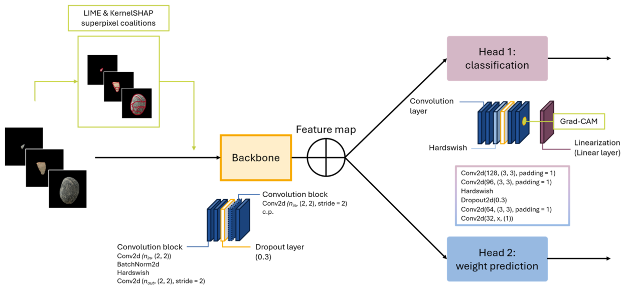
Figure 2.
Attribution maps of Grad-CAM, LIME and SHAP on four representative particles from small (4–5.6 mm), medium (16–22.4 mm) and large (31.5–45 mm, 45–63 mm) particle size classes (a) Attribution maps for the classification head. (b) Attribution maps for the regression head.
Figure 2.
Attribution maps of Grad-CAM, LIME and SHAP on four representative particles from small (4–5.6 mm), medium (16–22.4 mm) and large (31.5–45 mm, 45–63 mm) particle size classes (a) Attribution maps for the classification head. (b) Attribution maps for the regression head.
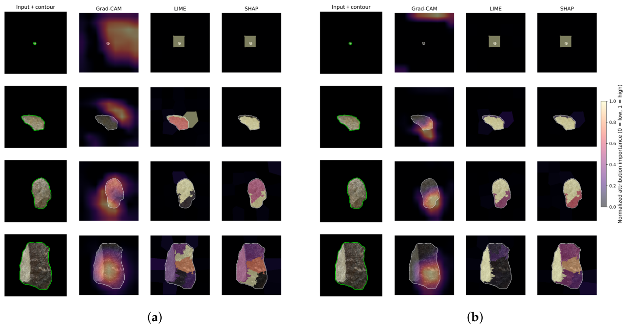
Figure 3.
Raincloud plots that show the distribution and median deletion AUCs, where lower is better. (a) Raincloud plot for the classification head deletion AUC (b) Raincloud plot for the regression head deletion AUC
Figure 3.
Raincloud plots that show the distribution and median deletion AUCs, where lower is better. (a) Raincloud plot for the classification head deletion AUC (b) Raincloud plot for the regression head deletion AUC
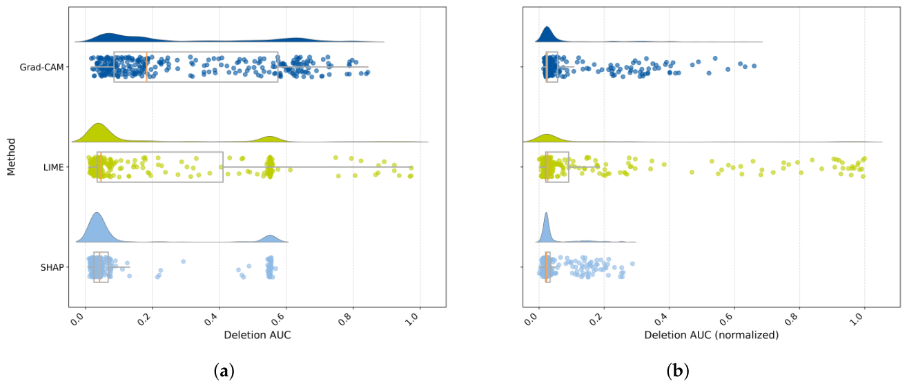
Figure 4.
Raincloud plots that show the distribution and median insertion AUCs, where higher is better. (a) Raincloud plot for the classification head insertion AUC (b) Raincloud plot for the regression head insertion AUC
Figure 4.
Raincloud plots that show the distribution and median insertion AUCs, where higher is better. (a) Raincloud plot for the classification head insertion AUC (b) Raincloud plot for the regression head insertion AUC
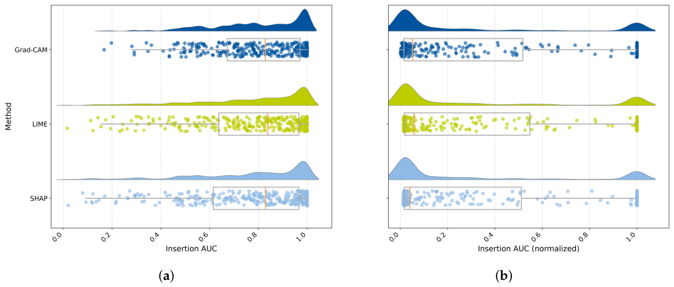
Figure 5.
Heatmaps of the median results for stability metrics , and . (a) Heatmap of the median global and values, i.e. considering all attribution pixels (b) Heatmap of the median , and values considering only the top-K (i.e. masks) attribution pixels. Abbreviations: = Pearson linear correlation; = Spearman rank correlation; = Kendall rank correlation; C = classification head; R = regression head.
Figure 5.
Heatmaps of the median results for stability metrics , and . (a) Heatmap of the median global and values, i.e. considering all attribution pixels (b) Heatmap of the median , and values considering only the top-K (i.e. masks) attribution pixels. Abbreviations: = Pearson linear correlation; = Spearman rank correlation; = Kendall rank correlation; C = classification head; R = regression head.
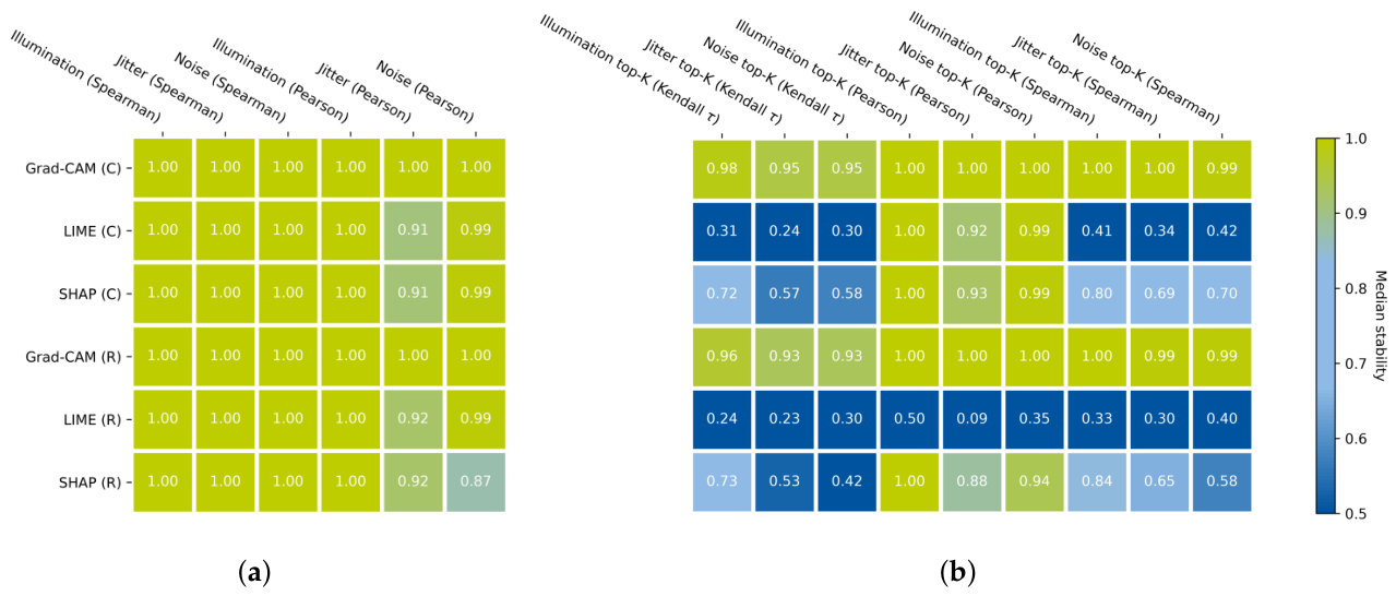
Figure 6.
Lineplots for the median localization RRA and IoU values per particle size class. (a) Median classification IoU (b) Median regression IoU (c) Median classification RRA (d) Median regression RRA. Abbreviations: IoU = intersection-over-union; RRA = relevance rank accuracy
Figure 6.
Lineplots for the median localization RRA and IoU values per particle size class. (a) Median classification IoU (b) Median regression IoU (c) Median classification RRA (d) Median regression RRA. Abbreviations: IoU = intersection-over-union; RRA = relevance rank accuracy
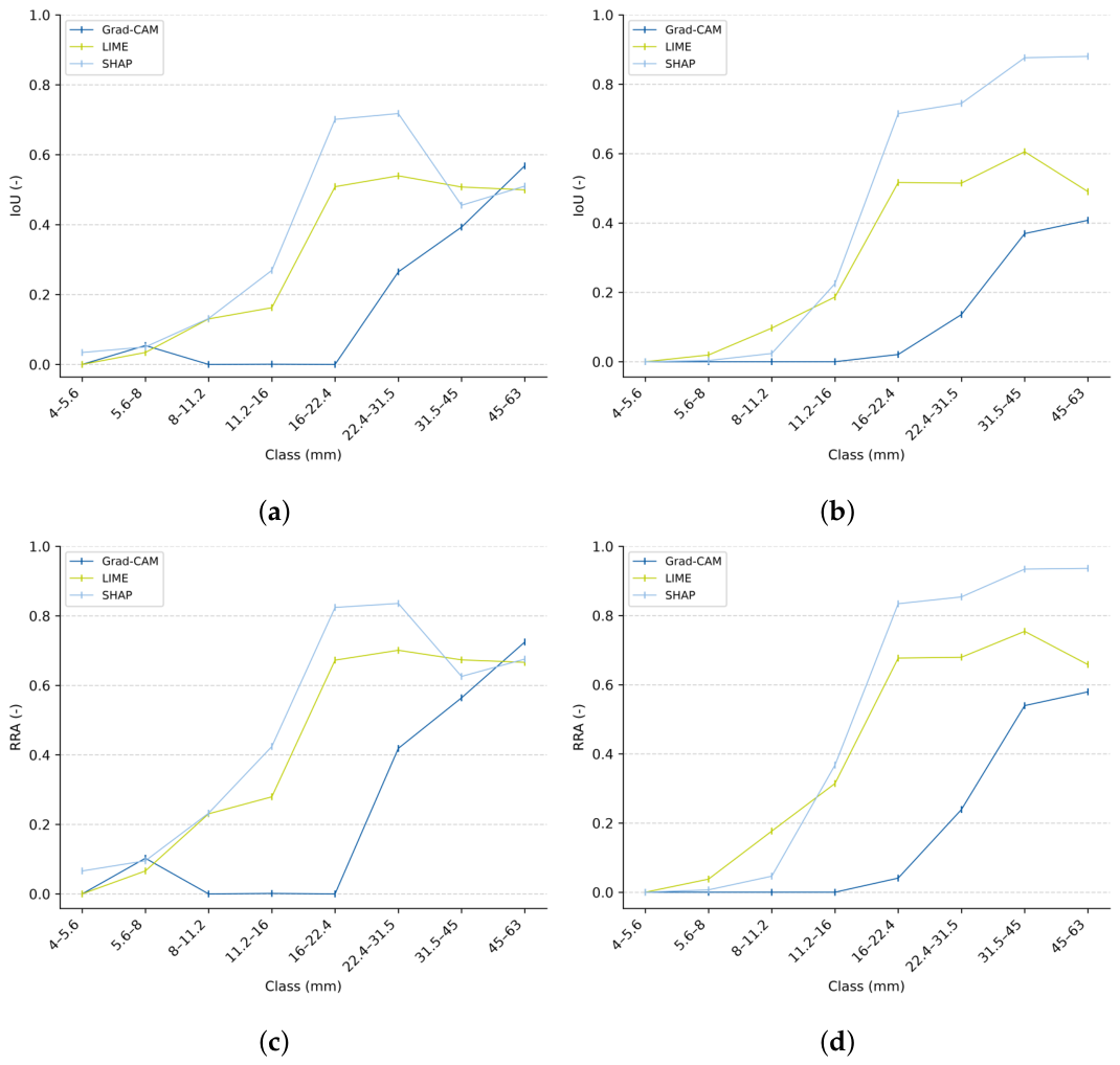
Figure 7.
Heatmap of the statistical significance results calculated using the pairwise Holm-corrected Wilcoxon test. (a) Statistical significance results for the classification head. (b) Statistical significance results for the regression head.
Figure 7.
Heatmap of the statistical significance results calculated using the pairwise Holm-corrected Wilcoxon test. (a) Statistical significance results for the classification head. (b) Statistical significance results for the regression head.
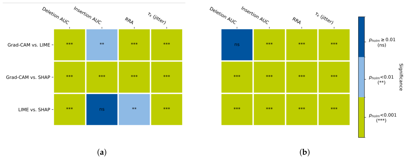
Figure 8.
Radar chart for the classification and regression head, containing the normalized results for each of the key evaluation metrics, where the more outward the value, the better the performance.
Figure 8.
Radar chart for the classification and regression head, containing the normalized results for each of the key evaluation metrics, where the more outward the value, the better the performance.
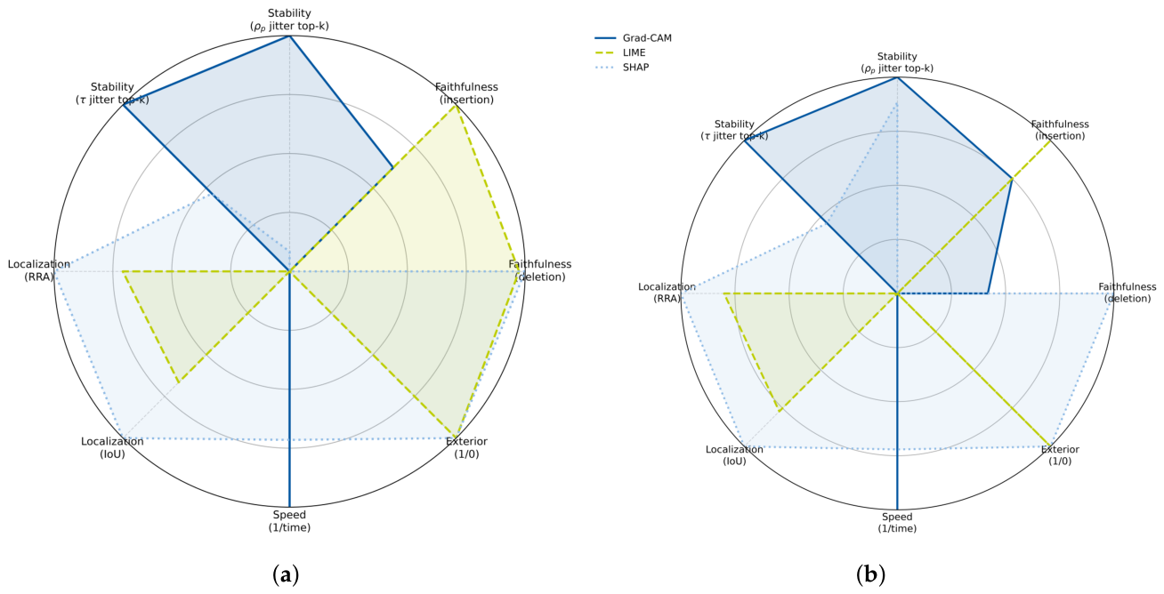
Table 1.
Number of particles used in the dataset for each class
| Class index |
Class (mm) |
Total nr. particles (-) |
Nr. particles in test set (-) |
|---|---|---|---|
| 1 | 4–5.6 | 260 | 52 |
| 2 | 5.6–8 | 200 | 40 |
| 3 | 8–11.2 | 199 | 40 |
| 4 | 11.2–16 | 200 | 40 |
| 5 | 16–22.4 | 200 | 40 |
| 6 | 22.4–31.5 | 157 | 32 |
| 7 | 31.5–45 | 103 | 21 |
| 8 | 45–63 | 151 | 31 |
Table 2.
Median RRA and IoU to evaluate localization for each method. Abbreviations: RRA = relevance rank accuracy; IoU = intersection-over-union; IQR = interquartile range
Table 2.
Median RRA and IoU to evaluate localization for each method. Abbreviations: RRA = relevance rank accuracy; IoU = intersection-over-union; IQR = interquartile range
| Method | RRA [IQR] | IoU [IQR] |
|---|---|---|
| Classification | ||
| Grad-CAM | 0.00 [0–0.35] | 0.00 [0–0.21] |
| LIME | 0.27 [0.08–0.65] | 0.16 [0.04–0.49] |
| SHAP | 0.36 [0.12–0.78] | 0.22 [0.06–0.64] |
| Regression | ||
| Grad-CAM | 0.00 [0–0.24] | 0.00 [0–0.14] |
| LIME | 0.24 [0.08–0.67] | 0.14 [0.04–0.50] |
| SHAP | 0.35 [0.01–0.87] | 0.22 [0.07–0.77] |
Table 3.
Median values of the deletion AUC, insertion AUC, RRA and top-K under different data regimes to assess robustness. Abbreviations: AUC = area under curve; Del. = deletion; Ins. = insertion; RRA = relevance rank accuracy; = Kendall rank correlation; Orig. = Original; Bal. = Balanced; L-sk. = Left-skewed.
Table 3.
Median values of the deletion AUC, insertion AUC, RRA and top-K under different data regimes to assess robustness. Abbreviations: AUC = area under curve; Del. = deletion; Ins. = insertion; RRA = relevance rank accuracy; = Kendall rank correlation; Orig. = Original; Bal. = Balanced; L-sk. = Left-skewed.
| Orig. | Bal. | L-sk. | |||||||
|---|---|---|---|---|---|---|---|---|---|
| Metric | Grad-CAM | LIME | SHAP | Grad-CAM | LIME | SHAP | Grad-CAM | LIME | SHAP |
| Classification | |||||||||
| Del. AUC | 0.18 | 0.05 | 0.04 | 0.17 | 0.05 | 0.04 | 0.45 | 0.05 | 0.04 |
| Ins. AUC | 0.83 | 0.84 | 0.83 | 0.85 | 0.85 | 0.83 | 0.80 | 0.81 | 0.80 |
| RRA | 0.00 | 0.28 | 0.36 | 0.04 | 0.38 | 0.46 | 0.00 | 0.19 | 0.28 |
| 0.95 | 0.24 | 0.57 | 0.95 | 0.28 | 0.59 | 0.95 | 0.23 | 0.57 | |
| Regression | |||||||||
| Del. AUC | 0.02 | 0.03 | 0.02 | 0.03 | 0.03 | 0.02 | 0.02 | 0.02 | 0.02 |
| Ins. AUC | 0.05 | 0.06 | 0.04 | 0.12 | 0.15 | 0.13 | 0.03 | 0.04 | 0.03 |
| RRA | 0.00 | 0.24 | 0.35 | 0.01 | 0.38 | 0.52 | 0.00 | 0.22 | 0.21 |
| 0.93 | 0.23 | 0.53 | 0.93 | 0.28 | 0.57 | 0.93 | 0.17 | 0.54 |
Disclaimer/Publisher’s Note: The statements, opinions and data contained in all publications are solely those of the individual author(s) and contributor(s) and not of MDPI and/or the editor(s). MDPI and/or the editor(s) disclaim responsibility for any injury to people or property resulting from any ideas, methods, instructions or products referred to in the content. |
© 2026 by the authors. Licensee MDPI, Basel, Switzerland. This article is an open access article distributed under the terms and conditions of the Creative Commons Attribution (CC BY) license.
Copyright: This open access article is published under a Creative Commons CC BY 4.0 license, which permit the free download, distribution, and reuse, provided that the author and preprint are cited in any reuse.