

Submitted:
17 October 2026
Posted:
19 October 2026
You are already at the latest version
Abstract
Elementary cellular automata (ECA) are deterministic systems whose global behavior depends on both local update rules and initial states. While local rules are simple, predicting global variability remains a challenge. Here, we quantify this variation across all 256 Wolfram rules using 100 independent random initial states per rule (width 200, 200 updates) and test whether local rule-table descriptors predict the variance. Using mean normalized LZ78 complexity as the trajectory-level outcome, we define the rule-level target as the standard deviation of this score across seeds. Under five-fold cross-validation grouped by symmetry equivalence classes, an enriched ridge model yielded an of 0.0157, demonstrating that local descriptors provide weak predictive performance for global variance. In an exploratory extension, we fit Gaussian mixtures to the LZ scores of ten previously selected rules. Across two lattice widths, held-out trajectories assigned to high- and low-complexity components exhibited repeatable differences in mean density, though a secondary damage-spreading measure showed no significant effects. These results characterize finite-size outcome variability and highlight a repeatable association between LZ-based complexity and density, without establishing distinct dynamical regimes or absolute limits on local prediction.
Keywords:
elementary cellular automata
; initial conditions
; LZ78
; cross-validation
; rule-table descriptors
; density
; reproducibility
1. Introduction
Elementary cellular automata are one-dimensional, binary cellular automata in which each cell updates synchronously from its state and the states of its two nearest neighbours. Despite the compactness of the local rule table, their space-time patterns vary widely. This diversity has motivated longstanding efforts to relate local descriptions to large-scale behaviour and to classify the resulting dynamics (Wolfram, 1983, 1984).
The initial state is part of this problem. Dhar et al. (1995) showed that qualitative classification can depend on the initial configurations used in simulations. Borriello and Walker (2017) developed an information-based classification that explicitly studies variation in transfer entropy across inputs. Initial-condition dependence is therefore an established research subject. The question addressed here is narrower. For a fixed operational measure of trajectory complexity, how much does its value vary across random initial states, and can a small collection of descriptors computed from the local rule table predict that variability when related rules are held out together?
The distinction between a rule-level mean and a rule-level spread matters. A rule can have a stable average score with appreciable seed-to-seed dispersion, or a similar average score with little dispersion. If local descriptors are used to anticipate global behaviour, their ability to predict these distributions is a separate empirical question from their ability to predict a mean or a qualitative class.
We first examine all 256 ECA rules under one fixed simulation protocol. The primary outcome is a finite-size normalized LZ78 phrase-count score computed row by row. We summarize its variation across initial conditions and test three rule-table models under cross-validation grouped by reflection/complement equivalence classes. We then report an explicitly exploratory analysis of LZ-score distributions for ten rules selected in earlier runs. That analysis asks whether training-fitted mixture assignments correspond to independent trajectory summaries on held-out seeds and at a second lattice width.
The study does not treat LZ78 as a universal definition of complexity. Nor does it assume that a mixture component represents an attractor or a distinct dynamical regime. These are operational measurements, and the conclusions are restricted accordingly.
2. Methods
2.1. Elementary Cellular Automata and Simulation Protocol
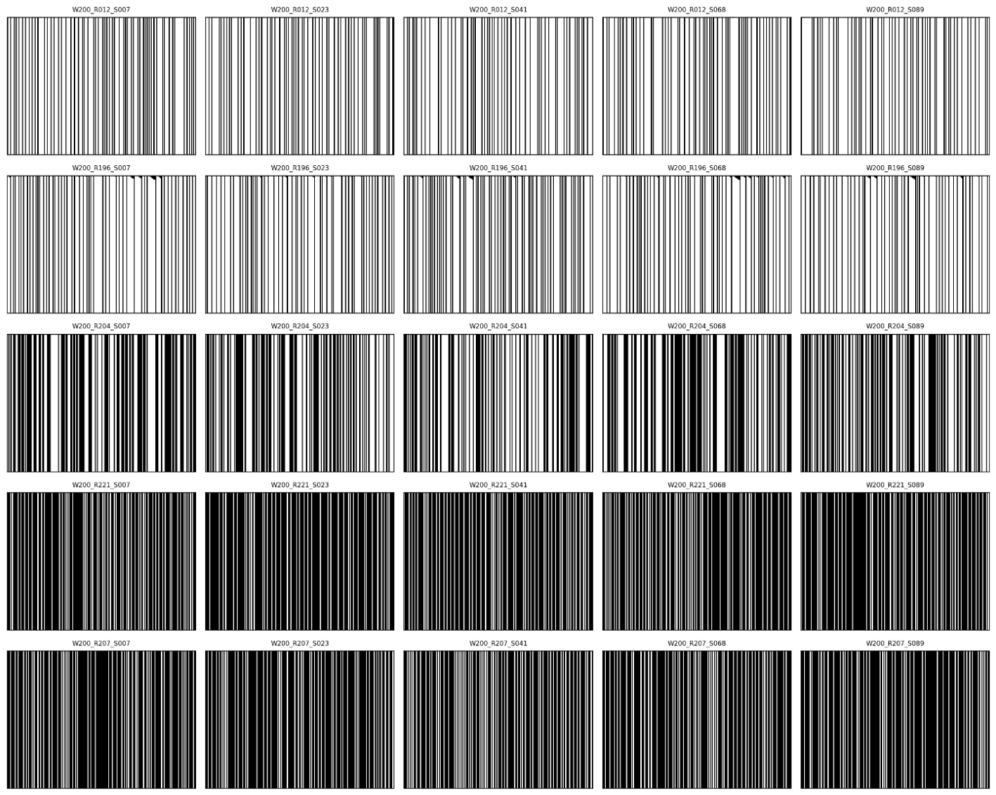
We simulated all 256 Wolfram-numbered elementary cellular automata. The lattice was one-dimensional with binary states, periodic boundary conditions, synchronous updates, and nearest-neighbour radius one. Each initial state was sampled independently from Bernoulli(0.5). The main experiment used width L = 200 and T = 200 updates, retaining the initial row and all evolved rows. There were 100 initial states per rule, for 25,600 trajectories. The recorded seed derivation and implementation are included in the accompanying code and data archive.
Figure 1.
Representative spacetime diagrams for selected elementary cellular automata rules and random initial conditions. The vertical axis represents time (200 updates), and the horizontal axis represents space (periodic lattice of width 200). The visual diversity demonstrates the dependence of global patterns on both the local rule and the specific initial state.
Figure 1.
Representative spacetime diagrams for selected elementary cellular automata rules and random initial conditions. The vertical axis represents time (200 updates), and the horizontal axis represents space (periodic lattice of width 200). The visual diversity demonstrates the dependence of global patterns on both the local rule and the specific initial state.
2.2. Trajectory Score and Across-Seed Variability
For each evolved row of length n = 200, we computed the LZ78 phrase count C(n) using incremental parsing and transformed it to C(n) log2(n) / n. The trajectory score was the arithmetic mean of this quantity across rows t = 1,...,200. The initial row was excluded. For each rule, the target was the sample standard deviation (ddof = 1) of the 100 trajectory scores. This is a finite-length, operational statistic. It is not an estimate of Kolmogorov complexity and should not be interpreted as a universal complexity scale.
The prediction target was log(SD + 0.001), where SD is the rule-level sample standard deviation. The offset allows rules with zero observed variability to remain in the analysis. It is part of the specified operational target.
2.3. Local Rule-Table Descriptors
The baseline model used the reflection/complement-invariant output density descriptor λ_sym = min(λ, 1 − λ), where λ is the fraction of rule-table outputs equal to one, and total Boolean sensitivity, defined as the sum of the three input-coordinate influences. The enriched model additionally used centre influence, mean left/right influence, and absolute left/right influence difference. These descriptors are computed from the rule table. Binary output entropy was not included as a separate predictor because it is a deterministic function of λ.
2.4. Symmetry-Aware Validation
The 256 rules were partitioned into 88 reflection/complement equivalence classes. Five-fold GroupKFold cross-validation used these classes as groups, so members of the same equivalence class were not split between training and test folds. Models were standardized ridge regressions with α = 1.0. No hyperparameter tuning was performed. A null predictor returned the training-fold mean. We report out-of-fold RMSE, MAE, and R² on log(SD + 0.001). The full scan and final feature choices were exploratory, informed by earlier pilot analyses; the validation was not externally preregistered.
2.5. Width-Specific Held-Out Component Analysis
A separate analysis used ten rules selected in earlier exploratory work: 12, 196, 204, 221, 207, 220, 100, 68, 69, and 206. This selection means the analysis is not an unbiased test over the full rule space. At each of widths 200 and 400, we generated 100 training and 200 held-out trajectories per rule. Initial states were Bernoulli(0.5), boundaries periodic, and T = 200. A two-component Gaussian mixture was fitted to the training trajectory LZ scores separately for each rule and width. The components were ordered by their fitted LZ means. The fitted model assigned held-out trajectories to the lower- or higher-mean component. Held-out density and damage summaries were not used to fit the mixture.
The primary independent outcome was mean density across evolved rows. Predefined secondary outcomes were the temporal standard deviation of row density and the mean single-cell damage fraction over updates 1–50. Damage was measured by flipping the middle cell in the initial state and comparing the resulting trajectory with the unperturbed trajectory. Within each rule, width, metric, and assignment subset, high- versus low-LZ component outcomes were compared with two-sided Mann–Whitney U tests. Benjamini–Hochberg correction was applied across rules within each width × metric × assignment subset. Results are shown for all hard assignments and as a sensitivity analysis restricted to posterior assignment confidence of at least 0.8. Because some rule-width mixtures produced insufficient group counts, not all rules contributed to every comparison.
This analysis is post hoc. The held-out seeds were independent of the corresponding mixture fit, but the ten rules were selected using earlier outcomes. The second width tests whether associations recur under width-specific mixtures; it does not test transfer of one width’s mixture model to the other width.
3. Results
3.1. Variation Across Initial Conditions
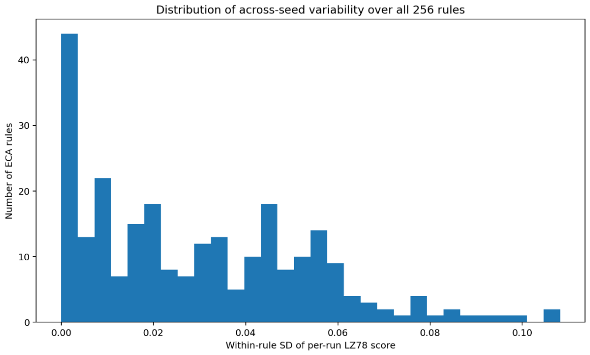
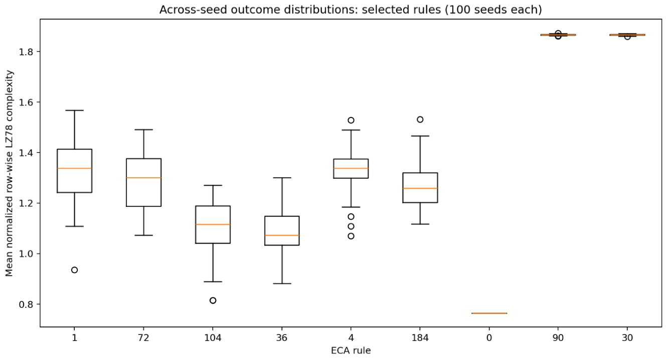
The mean within-rule sample standard deviation of the trajectory LZ score was 0.0301 across rules, with a standard deviation across rules of 0.0243. The median rule-level SD was 0.0258; the interquartile range was 0.00784 to 0.0470. Two rules had zero observed variability among their 100 seeds. Rule 1 had the largest observed SD (0.1082), followed by rules 72 (0.1050), 104 (0.0991), 233 (0.0953), and 127 (0.0917).
Figure 2.
Distribution of across-seed variability over all 256 elementary cellular automata. The histogram shows the number of rules falling into each bin of within-rule standard deviation of the mean LZ78 trajectory score. The distribution is heavily right-skewed, indicating that most rules have low variance while a few (e.g., Rule 1) exhibit extreme sensitivity to initial conditions.
Figure 2.
Distribution of across-seed variability over all 256 elementary cellular automata. The histogram shows the number of rules falling into each bin of within-rule standard deviation of the mean LZ78 trajectory score. The distribution is heavily right-skewed, indicating that most rules have low variance while a few (e.g., Rule 1) exhibit extreme sensitivity to initial conditions.
These values describe the selected metric, width, time horizon, and initial-state distribution.
Figure 3.
Across-seed outcome distributions for selected rules (100 seeds each). Boxplots show the median, interquartile range, and outliers for the mean normalized LZ78 complexity score. Rules with highly heterogeneous dynamics (e.g., Rule 1, 72, 104) show wide dispersions, while stable or highly chaotic rules show tightly clustered scores.
Figure 3.
Across-seed outcome distributions for selected rules (100 seeds each). Boxplots show the median, interquartile range, and outliers for the mean normalized LZ78 complexity score. Rules with highly heterogeneous dynamics (e.g., Rule 1, 72, 104) show wide dispersions, while stable or highly chaotic rules show tightly clustered scores.
3.2. Prediction from Local Descriptors
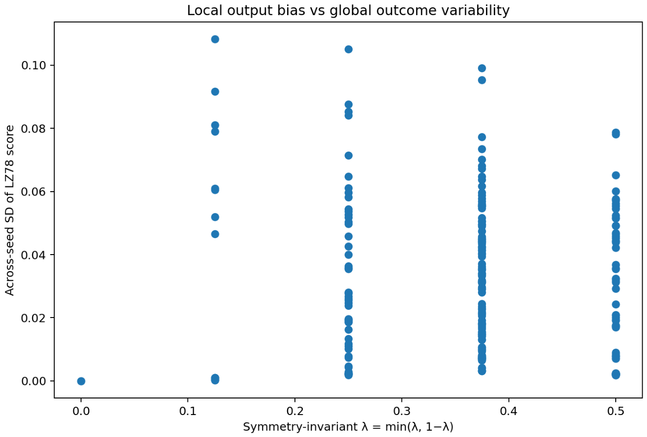
The null model achieved RMSE 1.1346, MAE 0.9502, and R² −0.0230 on the transformed target. The baseline model using λ_sym and total sensitivity achieved RMSE 1.1551, MAE 0.9594, and R² −0.0603. The enriched model achieved RMSE 1.1129, MAE 0.8882, and R² 0.0157. Its RMSE was approximately 1.9% lower than the null model’s. This is a small improvement and does not support a claim of useful prediction by these descriptors under the present design.
Figure 4.
Local output bias vs. global outcome variability. Scatter plot of the symmetry-invariant λ = min(λ,1 − λ) against the across-seed standard deviation of the LZ78 score for all 256 rules. The lack of a strong monotonic trend visually corroborates the low predictive performance (R2 ≈ 0.015) of the ridge regression model.
Figure 4.
Local output bias vs. global outcome variability. Scatter plot of the symmetry-invariant λ = min(λ,1 − λ) against the across-seed standard deviation of the LZ78 score for all 256 rules. The lack of a strong monotonic trend visually corroborates the low predictive performance (R2 ≈ 0.015) of the ridge regression model.
3.3. Held-out Component Analysis
In the all-assigned analysis, mean density differed between high- and low-LZ component assignments after within-metric Benjamini–Hochberg correction for 8 of 10 rules at width 200 (rules 12, 68, 69, 100, 196, 207, 220, and 221; adjusted p values ranged from 5.64 × 10⁻⁸ to 7.78 × 10⁻⁶). At width 400, 7 of the 8 rules with adequate group counts were significant (rules 12, 68, 69, 196, 206, 220, and 221; adjusted p values ranged from 8.21 × 10⁻¹⁸ to 0.00162). The eight rules testable at both widths showed the same direction of mean-density difference. Median absolute standardized mean differences were 0.823 at width 200 and 0.862 at width 400. These counts and adjusted p values were checked against the archived held-out test CSV.
The secondary outcomes were less consistent. No rule showed a corrected significant difference in damage AUC at either width. For temporal density variability, no rule was significant at width 200; at width 400, one of eight testable rules was significant in the all-assigned analysis (rule 206, adjusted p = 0.00989). This isolated result does not provide broad confirmation across independent dynamical outcomes.
Component counts and posterior confidence varied by rule and width. The width-400 results therefore apply to the subset with sufficient observations in both assigned components. The exploratory rule selection also limits generalization beyond these ten rules.
4. Discussion
The all-rule scan found substantial variation in the across-seed standard deviation of the chosen trajectory score. The selected local descriptors predicted that variation poorly. Under symmetry-grouped validation, the enriched model’s improvement over a training-fold mean was small. The result is best read as a limitation of this feature set and modeling choice. Other rule descriptors, target measures, or models may perform differently.
The component analysis offers a narrower observation. When LZ scores were divided by training-fitted mixtures for selected rules, held-out trajectories assigned to the two components often differed in their mean density. The direction of the density difference was consistent across widths among the eight rules testable at both widths. This is evidence of a repeatable association in this selected set. It is not sufficient to identify separate attractors, prove multimodality, or establish different dynamical regimes. A Gaussian mixture can divide a continuous, skewed, or otherwise non-Gaussian distribution. Density is also a basic property of the same trajectories from which LZ scores were computed, so the association may reflect a relationship between density and finite-row compressibility.
The secondary measures provide no broad corroboration. Damage AUC did not differ significantly after correction. Temporal density variability produced one corrected result at the larger width. These findings should be reported as such, without reclassifying the secondary metrics or altering their thresholds after inspection.
Several limitations shape the scope of inference. First, the LZ score is measured on rows of finite length and averaged over a finite horizon. Different widths, time horizons, or sequence-complexity estimators may yield different distributions. Second, the local feature set is deliberately small and does not exhaust possible summaries of the rule table. Third, the all-rule scan was exploratory rather than preregistered. Fourth, the ten rules in the component analysis were selected from earlier outcomes. Independent seeds protect the mixture fit from direct leakage from the test trajectories, but they do not remove selection of the rules. Finally, the damage metric uses one-cell perturbations and a 50-update window; it cannot represent every notion of dynamical sensitivity.
The appropriate next step is a new study in which rule selection, component criteria, effect-size thresholds, and primary independent dynamical outcomes are specified before data are examined. Such a study should include a rule-selection procedure independent of the present results and evaluate whether LZ component membership predicts more than density. Until then, the results support a careful account of variability and a density association, not a general theory of the relationship between local rules and emergent dynamics.
5. Conclusion
Across all 256 elementary cellular automata, a small set of symmetry-invariant local descriptors predicted across-initial-condition variation in a finite-size LZ78 trajectory score only weakly under the tested grouped cross-validation design. In a separate post hoc analysis of ten previously selected rules, training-fitted LZ mixture assignments were associated with differences in mean density on held-out trajectories. The predefined damage-spreading outcome did not provide comparable support, and temporal density variability yielded only one corrected result at the larger width. The mixture assignments do not establish multimodality or distinct dynamical regimes. These results motivate independent, preregistered evaluation of the density association.
Data and Code Availability: The accompanying archive contains simulation scripts, analysis scripts, trajectory-level CSV files, rule-level summaries, figures, tests, and configuration files. The code uses Python with NumPy, pandas, scikit-learn, SciPy, statsmodels, matplotlib, and pytest; Numba is optional for LZ parsing acceleration. The archive’s README provides execution instructions. Repository can be found at: 10.5281/zenodo.23432754.
References
- Borriello, E.; Walker, S. I. An information-based classification of elementary cellular automata; Complexity, 2017; p. 1280351. [Google Scholar] [CrossRef]
- Dhar, A.; Lakdawala, P.; Mandal, G.; Wadia, S. R. Role of initial conditions in the classification of the rule space of cellular automata dynamics. Phys. Rev. E 1995, 51(4), 3032–3037. [Google Scholar] [CrossRef] [PubMed]
- Lempel, A.; Ziv, J. On the complexity of finite sequences. IEEE Trans. Inf. Theory 1976, 22(1), 75–81. [Google Scholar] [CrossRef]
- Pita, M. How local rules generate emergent structure in cellular automata. arXiv 2026, arXiv:2604.00273. [Google Scholar] [CrossRef]
- Wolfram, S. Statistical mechanics of cellular automata. Rev. Mod. Phys. 1983, 55(3), 601–644. [Google Scholar] [CrossRef]
- Wolfram, S. Universality and complexity in cellular automata. Physica D. Nonlinear Phenom. 1984, 10(1–2), 1–35. [Google Scholar] [CrossRef]
Disclaimer/Publisher’s Note: The statements, opinions and data contained in all publications are solely those of the individual author(s) and contributor(s) and not of MDPI and/or the editor(s). MDPI and/or the editor(s) disclaim responsibility for any injury to people or property resulting from any ideas, methods, instructions or products referred to in the content. |
© 2026 by the author. Licensee MDPI, Basel, Switzerland. This article is an open access article distributed under the terms and conditions of the Creative Commons Attribution (CC BY) license.
Copyright: This open access article is published under a Creative Commons CC BY 4.0 license, which permit the free download, distribution, and reuse, provided that the author and preprint are cited in any reuse.