

Submitted:
15 October 2026
Posted:
16 October 2026
You are already at the latest version
Abstract
Population estimation methods in routine use (FOCE-I, SAEM, importance-sampling EM) assume that model predictions vary smoothly with the individual parameters. That makes residuals informative and lets the individual likelihood be approximated locally. Both assumptions fail for chaotic structural models, which matter more and more for oscillatory pharmacodynamic systems such as hormone pulsatility and glucose–insulin dynamics. We present a reproducible two-stage pipeline and test it on an intentionally challenging benchmark: 16 Lorenz-63 subjects with log-normal inter-individual variability (IIV), a bimodal population straddling a bifurcation (8 chaotic, 8 periodic), one observed state, and 20% proportional residual error. Stage 1 replaces residual-based likelihoods with feature matching by the simulated method of moments, using features scaled to each subject’s own oscillation period. It also replaces covariance-based standard errors, which inflated the IIV of the weakly identified parameter σ more than five-fold, with objective-function profiles. The scale of these profiles is calibrated per regime by simulating at the subject’s own estimates. Stage 2 combines the profiles in exact-grid or Gibbs hierarchical posteriors, including a mixture model analogous to NONMEM $MIXTURE. Diagnostics include feature-based, marginal-quantile, and peak-aligned visual predictive checks (VPCs), EBEs with shrinkage, and Lyapunov classification. The method recovered the residual error (0.1992 vs 0.200), mixture fraction (0.500 vs 0.500), σ typical value (10.04 vs 10.12), and β IIV (0.057 vs 0.052), and cut individual-estimate EBE error five-fold with respect to the Stage 1 estimates. The IIV of σ was underestimated (0.017 vs 0.032). Chaotic subjects carry almost no information on σ (93% shrinkage), so this estimate effectively reflects the periodic subpopulation. Peak-aligned VPCs passed in the periodic stratum (9% of points outside the 90% intervals) but not in the chaotic stratum (20%), indicating residual misspecification.
Keywords:
nonlinear mixed-effects models
; chaotic dynamics
; simulated method of moments
; profile likelihood
; identifiability
1. Introduction
1.1. What the Population Approach Assumes
Population modeling rests on a hierarchy familiar to pharmacometricians: individual parameters are drawn from a population distribution described by typical values and IIV variance components (THETA and OMEGA); individual observations arise from a structural model plus residual unexplained variability (RUV; SIGMA); and estimation maximizes an approximation to the marginal likelihood or samples the posterior [1,2]. Every traditional estimation algorithm— FO, FOCE-I, Laplacian, SAEM, IMP — exploits the same property of : it is a smooth function of . That is what makes individual residuals informative, and goodness-of-fit plots meaningful, and what allows the conditional likelihood to be linearized or sampled around a well-defined mode.
1.2. Where Chaotic Systems Break It
A growing class of pharmacodynamic systems violates this property. Systems such as ultradian hormone secretion, glucose–insulin feedback, intracellular calcium signaling and circadian readouts are governed by nonlinear oscillators that can operate in periodic or chaotic regimes, and patients may plausibly be distributed on both sides of the boundary [3,4,5]. When the dynamics are mixed laminar/chaotic, three issues may arise:
- Residuals carry no information. Two subjects with almost identical parameters may produce completely different trajectories after a short time, so even at the true parameters the prediction does not track the data. IPRED, CWRES, and the whole goodness-of-fit apparatus lose meaning.
- The objective function is jagged. Plotted against any parameter, the objective shows many small dips rather than one smooth local quadratic. FOCE-type linearization and the $COV step both assume a local quadratic.
- The population is bimodal, and the two groups are unequally informative. A single log-normal distribution cannot describe two clusters, and periodic subjects reveal some parameters much more precisely than chaotic ones, so treating every subject’s information on one common scale may mis-weight the two groups.
1.3. What this Paper Does
We describe a pipeline and a Julia script that address all three failures on a fully controlled benchmark where the truth is known. The method is a two-stage method in the lineage of the standard and global two-stage approaches (STS, GTS) [6]: each subject is fitted separately, then the individual results are combined into a population model. What differs is that each component GTS relies on — the individual objective, the carrier of individual uncertainty, and the scale of that uncertainty — is replaced by one that survives chaos. The design philosophy is truth-free operation with embedded validation: every quantity used for inference is computable from observed data alone; the known truth is used only in blocks explicitly marked “[validation]”, the simulation-study analog of keeping analysis and evaluation data separate.
2. Methods
2.1. The Benchmark
Structural model. Each subject follows the Lorenz-63 system
IIV model. Log-normal about regime-specific typical values — like a NONMEM $MIXTURE model with two subpopulations [9]. The periodic window is interleaved with chaotic bands, so sampling alone does not guarantee regime membership; each periodic candidate was verified dynamically (largest Lyapunov exponent , Benettin algorithm [10]) and redrawn if it failed. Five periodic candidates were rejected in the reported run.

Table 1.
Study design.
| Element | Value | Related concept |
|---|---|---|
| Subjects | N = 16, stratified 8 chaotic / 8 periodic | Small study with two subpopulations |
| Nominal values | σ = 10, β = 8/3; ρ = 28 (chaotic) or 156 (periodic) | THETA by subpopulation |
| Design IIV (SD on log scale) | σ 0.05, β 0.05, ρ 0.02 | OMEGA |
| Observations | z only, 4000 samples, Δt = 0.01, T = 40 time units after a 50-unit run-in | Rich sampling, one analyte, after burn-in |
| Residual error model | proportional, exponential form, b = 0.20 | 20% CV exponential RUV |
| Integration method | RK4, step 0.0025 | ADVAN13-type numerical integration |
Two points for the reader. First, the realized standard deviations of the 16 sampled subjects differ from the design values; the validation targets throughout are the realized values (log : mean 2.3150, SD 0.0319; log : mean 0.9755, SD 0.0516), because that is what is in the data. The realized SD of log is itself regime-dependent: 0.023 among the eight periodic subjects and 0.041 among the eight chaotic subjects, a fact that matters for the interpretation of (Section 4). Second, for legibility, Figure 1 shows only the first 8 time units; the analysis window is 40 units.
A preflight block validates the dynamical substrate before any estimation: Lyapunov spectra at both regime centers ( = 0.895 chaotic, −0.009 periodic), the trace identity as an integration check (error ), the subcritical Hopf point , and a bisection estimate of the periodic-window edge (166.06 vs the literature value 166.07).
2.2. Overview of the Pipeline
2.3. Step 1: Residual-Error Model Estimated from the Raw Data
Observations follow
Table 2.
Steps, their purpose, and related concepts.
| Step | What is done | Why | Related concept |
|---|---|---|---|
| 1 | Estimate residual error from raw data (third differences) | Model residuals are meaningless under chaos | Estimating assay errors from replicates rather than from IWRES |
| 2 | Smooth each series and summarize it into 25 features, with time lags expressed in units of the subject’s own period; apply identical processing to every simulated series | Point-wise matching is challenging; matching features is not | NCA metrics (Cmax, inter-dose interval, fluctuation); pcVPC-style symmetric correction |
| 3 | Assign each subject a provisional regime label from the data alone | Needed to calibrate per regime and stratify diagnostics | Pre-classifying subjects by phenotype |
| 4 | Fit each subject by matching simulated to observed features (28 starting points) | Individual estimates | Individual fits with many initial estimates, keeping the lowest OFV |
| 5 | Compute conventional SEs (curvature, bootstrap) as comparators | Demonstrate they fail | $COV step; PsN bootstrap |
| 6 | Map each subject’s objective over σ (profile) | Keeps all information, including second dips | PsN llp for every subject |
| 7 | Re-fit when the profile reveals a lower minimum | Repairs optimizer misses | Re-running after llp shows a lower OFV |
| 8 | Calibrate the profile scale by simulating at subjects’ own estimates | The objective is not an OFV; its scale is unknown | A small SSE checking that ΔOFV thresholds are correct |
| 9 | Population distribution of σ on an exact grid | THETA/OMEGA for σ | $EST for one parameter, with credible interval(s) |
| 10 | Two-subpopulation model for ρ; robust GTS for β | THETA/OMEGA for ρ, β | $MIXTURE NSPOP=2; GTS |
| 11 | EBEs, shrinkage, ETABAR | Individual estimates | POSTHOC, η-shrinkage |
| 12 | Feature VPCs, observation-scale VPCs, individual predictive checks, dynamical checks, virtual populations | Model evaluation | VPC, pcVPC, NPDE, simulation-based checks |
| 13 | Repeat everything with the true residual error (“oracle arm”) | Cost of estimating RUV | SSE with SIGMA fixed to truth |
Table 3.
Residual-error estimation (truth-free), with validation.
| Quantity | Estimate | Truth | Comment |
|---|---|---|---|
| b (pooled) | 0.1992 | 0.200 | relative error 0.4% |
| b (median per-subject) | 0.1994 | 0.200 | per-subject range 0.190–0.207 |
| a² (regression) | −17.9 → a used = 0 | 0 | pure proportional model correctly selected |
2.4. Step 2: Denoising and Feature Extraction, Applied Symmetrically
Each series is log-transformed and smoothed with a Daubechies-4 wavelet (5 levels, periodic boundary, soft thresholding with the single universal threshold [11]). In plain terms, the signal is split into a slow trend plus layers of finer detail, and fine details smaller than the noise level are removed. The smoother flattens peak tops slightly and leaves a lag-1 autocorrelation of 0.34 in standardized residuals; this does not matter, because of simulation symmetry: every simulated series passes through the same smoother with the same and the same subject-specific settings as the observed series, so the distortion cancels in the comparison. This is the logic of the prediction-corrected VPC [12]: a biased transformation is acceptable if applied identically to both sides.
From the smoothed series , 25 features are computed (Table 4). Two subject-specific constants are derived once from the observed smoothed series and then reused for every simulation of that subject. The first is the dominant period , taken from the first positive maximum of the autocorrelation function of (61–63 samples for the periodic subjects, 76–79 samples for the chaotic ones). The second is the peak-exclusion radius ; peaks are located as local maxima with greedy exclusion of neighbors within minsep.
Period-scaled signal-memory lags. The three autocorrelation features of are evaluated at lags of , and (9/31/62 samples for a typical periodic subject, 12/39/78 for a typical chaotic one). In the previous version of this pipeline, these lags were fixed at 10, 25, and 50 samples for every subject; the lag-25 feature then sat on the steep descending flank of the autocorrelation function between its zero crossing and its minimum, where a small difference in period between an observed subject and a virtual subject produces a large difference in the feature, and it was flagged in three of four stratified feature VPCs. Lags of and sit at the minimum and the next maximum of the autocorrelation function, where it is stationary, so the features measure waveform shape (depth of the anti-correlation, strength of the recurrence) rather than period; the lag retains short-lag sensitivity to waveform sharpness. Simulation symmetry is preserved because is fixed from the observed series during fitting; in the VPC, each virtual subject uses its own , exactly as each observed subject does.
Table 4.
The 25-element feature vector.
| Group | Features | Related concept |
|---|---|---|
| Level and spread | mean(z̃), SD(z̃), 10th and 90th percentiles of z̃ | Mean level, Cmin/Cmax |
| Peak amplitudes | mean, SD, 10/50/90th percentiles, CV of peak heights | Cmax statistics, fluctuation |
| Peak timing | mean and SD of inter-peak interval | Inter-pulse interval |
| Peak sequence memory | autocorrelation of the peak-height sequence at lags 1–8 | Regularity of successive peaks |
| Signal memory | autocorrelation of l̃ at lags 0.15 P, 0.5 P, 1.0 P (P = dominant period) | Shape of the oscillation, in units of its own period |
| Return map | slope and residual scatter of peak(k+1) vs peak(k) | Predictability of the next peak |
2.5. Step 3: Truth-Free Regime Label
Each subject receives a provisional label from three discriminators combined by majority vote: (i) the CV of peak amplitudes (periodic orbits have near-constant peaks; a gap-based cut at log cv_pk = −2.17), (ii) the dominant period, and (iii) the permutation entropy [13] of the smoothed log series (every 4th sample, embedding dimension 4, delay 2), oriented by (i). Two popular chaos tests — the 0–1 test [14] and a return-map periodicity score — are reported but excluded from the vote because they are unreliable on short noisy series.
Table 5.
Regime labeling: agreement with the true regime (validation).
| Discriminator | Correct / 16 | Used in vote |
|---|---|---|
| CV of peak amplitudes | 16 | yes (anchor) |
| Dominant period (cut 69.5 samples) | 16 | yes |
| Permutation entropy (cut 0.753) | 16 | yes |
| 0–1 test | 8 | no (negative control) |
| Return-map periodicity score | 7 | no (negative control) |
| Majority label | 16 | — |
The labels are used only to choose the calibration constant (Step 8) and to stratify diagnostics. They never restrict the search: every subject is fitted from starting points in both regimes , so a mislabeled subject can still converge to the correct regime, and a mismatch between label and fitted regime is a genuine diagnostic (Section 3.6).
2.6. Step 4: Individual Estimation by Feature Matching (Stage 1)
For a candidate , the model is simulated times with fresh residual noise and random initial states, each simulation is processed exactly as the data, and the features are averaged to give . The individual objective is the weighted squared distance between observed and simulated features:
This is the simulated method of moments (SMM) of McFadden and Gouriéroux–Monfort [15,16]. In NONMEM terms: adjust the parameters until simulated NCA summaries match the observed ones, weighting each summary by how reproducible it is. Two technical details matter:
- Common random numbers. The same 20 random seeds are reused every time is evaluated for a subject (as one fixes the seed in $SIMULATION). Otherwise would change between evaluations purely by chance and the optimiser would chase noise.
- Two-step weighting. A first pass uses a diagonal (inverse simulated feature variances). A second pass uses a full matrix estimated from 128 simulations at the first-pass estimate,
Search. Because is jagged, each subject is fitted from 28 starting points (7 values × 2 values × 2 regime centres) with Nelder–Mead (≤ 320 evaluations). The five best are refined under the full , and two further restarts are made from perturbed copies of the winner. A multimodality census — the number of distinct near-best solutions within 25 J-units of the best — is reported per subject.
2.7. Step 5: Conventional Standard Errors, Kept as Comparators
Two conventional individual covariances are computed: the curvature-based covariance with by central differences (the GMM asymptotic covariance; called “sandwich” in the code), and a parametric bootstrap (24 refits of synthetic data simulated at ). Feeding these into Stage 2 is the conventional GTS approach. Showing that it fails is a main result (Section 3.3).
2.8. Step 6: The -Profile as the Carrier of Individual Uncertainty
For each subject, is fixed at 33 points spanning 4–20 (plus up to 4 adaptive refinement passes near the minimum), and is minimized over at each point:
The profile is computed by continuation (each node warm-started from its neighbor), with fallback restarts and a smoothing sweep so that an isolated optimizer failure cannot leave a spurious spike. This is like llp for every subject across the whole plausible range [17]. The values along the profile are retained and later used to condition the and EBEs on the EBE.
2.9. Step 7: Multi-Basin Refinement
If a subject’s profile minimum undercuts its Stage 1 objective by more than 3.84, the optimizer missed the true minimum. The fit restarts from every competitive profile basin (within 7.68 of the minimum, up to four), keeps the best result, recomputes the weight matrix, bootstrap, and profile, and repeats the process for up to three rounds. In the reported run this repaired two optimizer failures in one round (Section 3.2) and left flat-profile subjects untouched — their problem is identifiability, not search, and is handled by shrinkage.
2.10. Step 8: Simulation Calibration of the Profile Scale
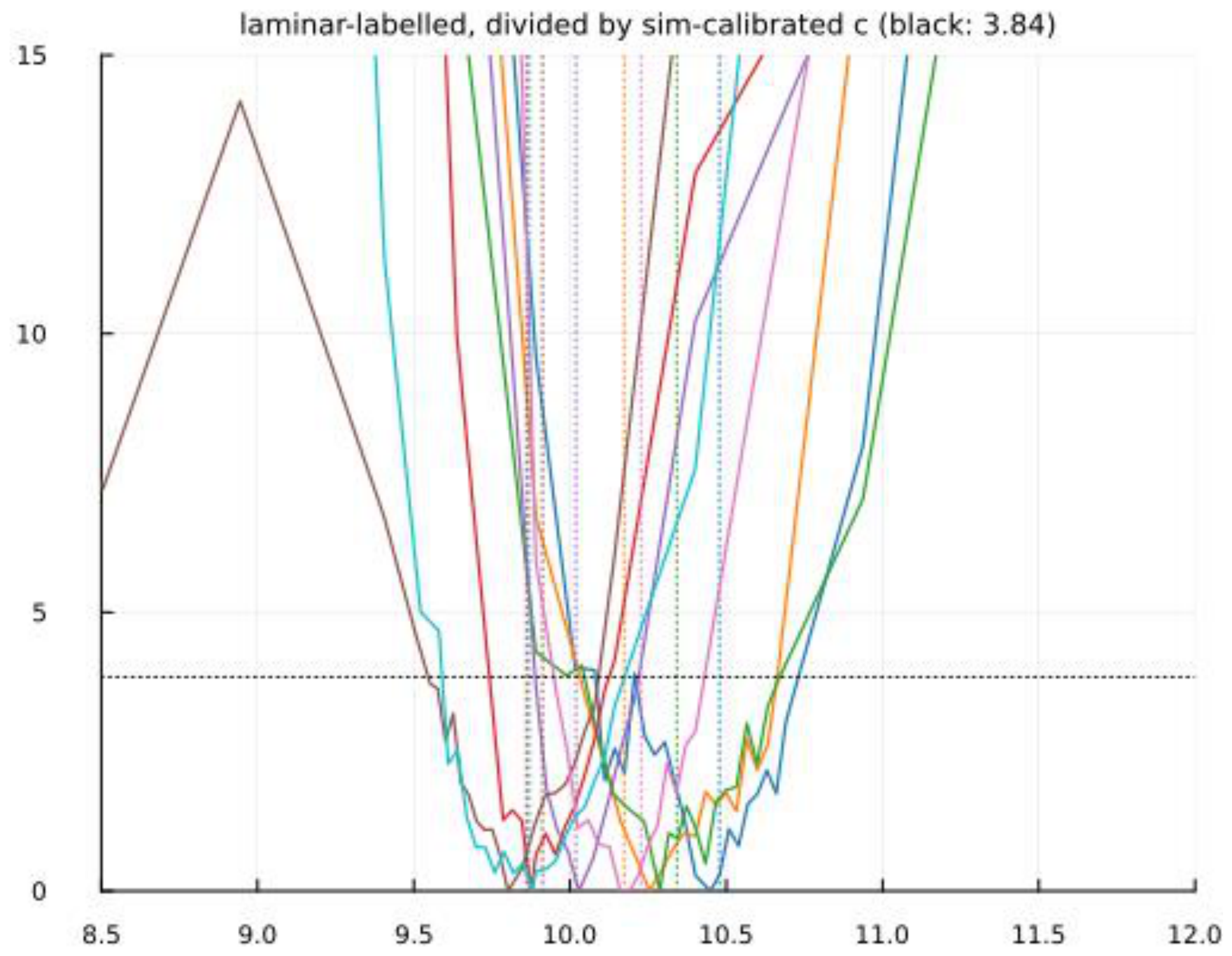
If were a true −2 log-likelihood, the familiar rules would apply: = 3.84 would be a 95% limit for one parameter, and at the true parameters would follow a distribution (median 2.366) for three parameters. But is a weighted feature distance, not an OFV, and its scale is unknown and regime dependent. Using it uncalibrated is exactly the situation in which an over-steep objective produces confidently wrong IIV estimates.
The pipeline measures the scale by a self-experiment that needs only the subjects’ own estimates:
- For each regime label, pick three representative subjects (lowest, middle and highest ) and simulate two synthetic datasets each at under the estimated RUV model — so the generating value is known.
- Refit each synthetic dataset with the full 28-start search plus one start at the generating value (guaranteeing ).
- Record and set
The profile then enters Stage 2 as the pseudo-likelihood
Reading the result: = 2.82 means the laminar objective is about 3× too steep; dividing by flattens those profiles so that the (very precise-looking) periodic subjects do not dominate the population fit — exactly as an overstated individual precision distorts a GTS analysis. The median is used rather than the mean because single refits can land in a remote basin: in the oracle arm, one chaotic refit ran to the upper bound with = 477, which would have driven a mean-based to its ceiling of 25. In NONMEM terms: a small SSE at your own final estimates, used to check that ΔOFV thresholds mean what they should, and to correct them if not. Because the experiment uses only subjects’ own estimates, it applies to real data.
2.11. Step 9: Population Distribution of (Stage 2, Exact Grid)
With , the marginal posterior of the hyperparameters under a flat prior is
evaluated exactly on a grid (1601 points in , 161 in , 150 in ) with no approximation and no Monte-Carlo error. The reported estimate is the posterior mean, with a 95% credible interval (the Bayesian counterpart of a CI). This is the analog of the NONMEM process: THETA and OMEGA for one parameter by exhaustive search instead of a gradient optimizer, with the output of a BAYES run. Because each subject contributes its whole profile, a subject with a broad or two-dip profile adds little certainty and cannot inflate artificially.
The same methodology is applied with alternative individual likelihoods — Gaussian with curvature covariance (GTS-like), with bootstrap covariance, and profiles with = 1 — to produce the “methods ladder” of Section 3.3.
2.12. Step 10: Two-Subpopulation Model for , Robust GTS for
For , each subject’s Stage-1 estimate with bootstrap variance enters a two-component mixture,
fitted by Gibbs sampling (16 000 iterations, 2 000 burn-in): alternately assign each subject to a component given the current component parameter, then update the component means, IIVs and the mixing fraction given the assignments; the label-switching ambiguity is removed by ordering . The output is the direct analog of $MIXTURE NSPOP=2: , two typical values, two IIVs and per-subject membership probabilities (MIXEST). A single log-normal fit (M1) is retained as a deliberate negative control. For , a GTS-type fit uses a heavy-tailed () individual likelihood centered on with bootstrap variance, on an exact grid.
2.13. Step 11: EBEs and Shrinkage
The EBE is the posterior mean of subject ’s profile combined with the fitted population distribution, integrating over hyperparameter uncertainty:
with a 90% interval from the quantiles of . For and , the profile values at are read off and shrunk towards the population (for , the membership-weighted component means) by the usual precision-weighted formula
Unconditioned EBEs (shrinking the Stage-1 , directly) are also reported, because the conditioning step turns out to be deleterious for subjects whose profile is flat (Section 3.6). η-shrinkage is , and ETABAR tests the mean η against zero, with their usual interpretation [18].
2.14. Step 12: Diagnostics on the Scale at Which the Model Is Fitted
- Feature VPC. 80 virtual subjects are simulated from each fitted population model (M1 single Gaussian ; M2 mixture; M2T mixture truncated to the regime of each component); for six features (mean, SD, mean peak, CV of peaks, mean inter-peak interval, ACF at 0.5 P) the observed median across the subjects in a stratum is compared with the 90% prediction interval of the median of an equal number of resampled virtual subjects, pooled and stratified by component. Stratification serves as a prediction correction.
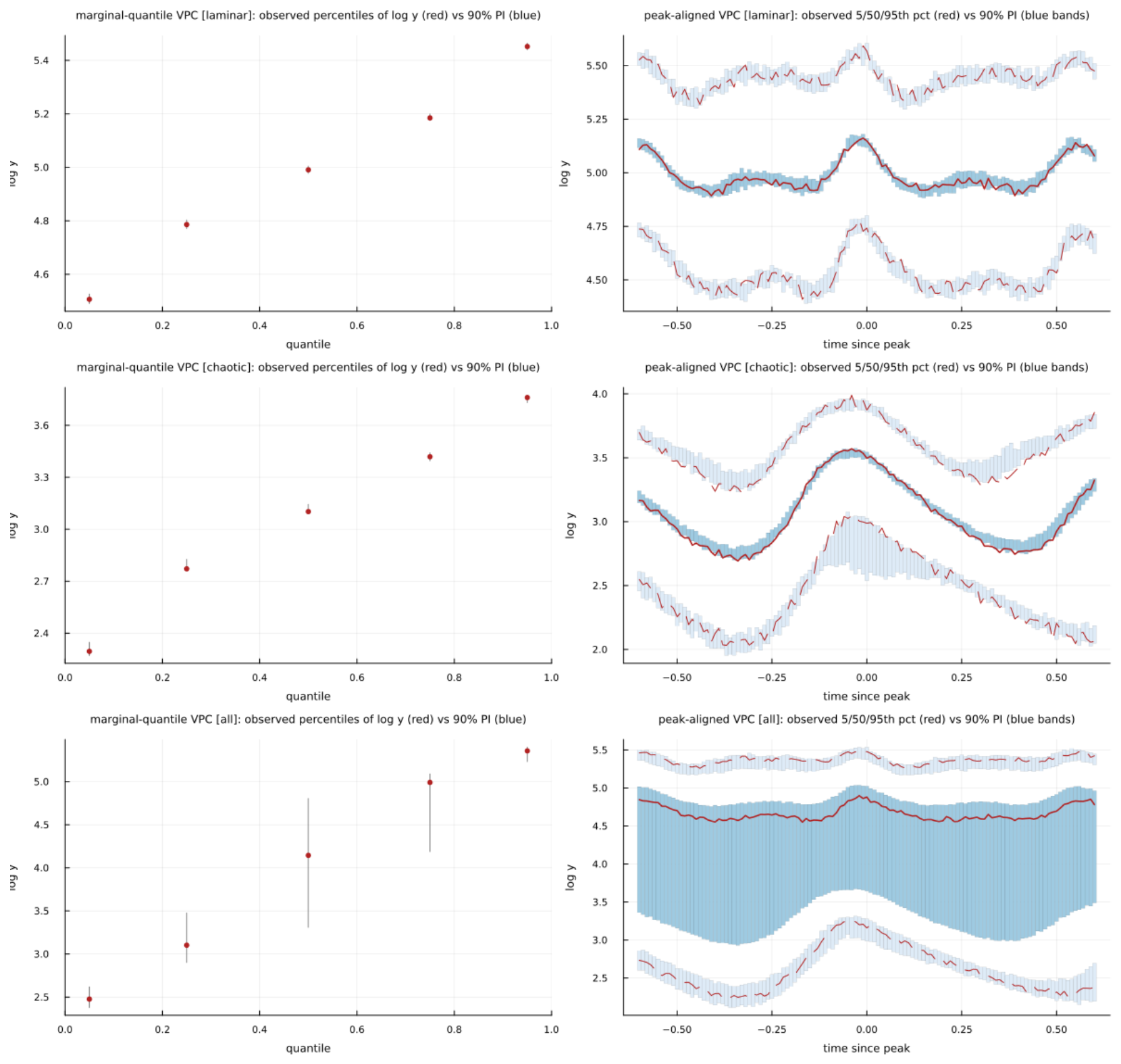
- Observation-scale VPCs. Because a time-indexed VPC is hard to interpret under chaos, we produce two valid substitutes from the M2T population. (a) A marginal-quantile VPC: the 5/25/50/75/95th percentiles of all observed in a stratum are compared with the 90% prediction interval of the same percentiles from 300 replicate virtual populations of the same size. (b) A peak-aligned VPC: every observed and simulated series is cut into windows centered on its detected peaks (± 0.6 time units; peaks located on the denoised series with the same rule as the features), and the 5th, 50th and 95th percentiles of raw as a function of time-since-peak are compared with their prediction intervals,
This is the event-aligned analog of a dose-aligned steady-state VPC. Both are produced per stratum (data label for observed subjects, mixture component for virtual subjects) and pooled; the pooled version is included to show what happens when a bimodal population is not stratified.
- -
- Individual predictive check. 32 simulations at each subject’s EBE; standardized feature residuals (observed − simulated mean)/simulated SD, summarized as mean |z| (≈ 0.8 for an adequate model).
- -
- Dynamical classification at the EBEs. The Lyapunov spectrum is computed at each EBE; an estimate that fits the features but crosses the bifurcation boundary is flagged.
- -
- Regime composition of virtual populations. Simulated subjects are classified; a model that places probability mass between the two modes produces infeasible fixed-point subjects. For M2T the mixture component is drawn once per virtual subject and only is redrawn within that component until it is regime-consistent, so the mixing fraction is preserved.
2.15. Validation Design
The whole of Steps 4–11 is run twice: with the estimated RUV (“estimated arm”) and with the true RUV (“oracle arm”). The difference measures the cost of estimating the residual-error model. The true parameters are otherwise used only in blocks marked [validation]. An automated verdict rule compares the two arms on the credible interval and the EBE coverage (failure threshold 12/16, the 5th percentile of a Binomial (16, 0.9)). The run (16 subjects, two arms, roughly 1 500 SMM optimizations plus the simulation-based diagnostics) took 52 min with 12 threads on a Lenovo P16 laptop under the Windows 11 operating system.
3. Results
3.1. Stage 1 Estimates and Multimodality
Chaotic subjects show 7–13 competitive minima in ; periodic subjects 1–4. and are well determined in both regimes (stage-1 RMSE in log 0.007, log 0.019). is not: stage-1 RMSE in log is 0.151 (≈ 15%), with two chaotic subjects (3 and 12) far from the truth ( 12.1 and 17.9 vs 10.5 and 10.4) on essentially flat profiles, and two more (7 and 8) 10–15% low. The eight periodic estimates are all within 2% of their true values.
Table 6.
Stage 1 estimates (estimated-RUV arm, after refinement) with the multimodality census.
| id | true regime | true | |||||
|---|---|---|---|---|---|---|---|
| 1 | periodic | 10.45 | 156.2 | 2.70 | 12.9 | 3 | 10.48 |
| 2 | periodic | 10.25 | 158.4 | 2.71 | 5.0 | 2 | 10.17 |
| 3 | chaotic | 12.07 | 27.0 | 2.63 | 13.3 | 13 | 10.49 |
| 4 | chaotic | 9.89 † | 28.4 | 2.94 | 12.4 | 12 | 10.29 |
| 5 | periodic | 10.29 | 161.0 | 2.51 | 11.3 | 3 | 10.34 |
| 6 | chaotic | 9.63 | 27.0 | 2.56 | 9.3 | 10 | 10.42 |
| 7 | chaotic | 9.08 | 27.7 | 2.69 | 17.1 | 8 | 10.07 |
| 8 | chaotic | 8.29 † | 29.1 | 2.71 | 16.2 | 11 | 9.70 |
| 9 | periodic | 9.88 | 156.6 | 2.79 | 8.6 | 1 | 9.86 |
| 10 | periodic | 10.03 | 160.5 | 2.77 | 7.9 | 1 | 10.02 |
| 11 | chaotic | 9.27 | 28.2 | 2.74 | 8.6 | 9 | 9.39 |
| 12 | chaotic | 17.87 | 28.7 | 2.29 | 5.4 | 12 | 10.37 |
| 13 | periodic | 9.80 | 150.5 | 2.56 | 7.7 | 2 | 9.91 |
| 14 | periodic | 10.16 | 160.2 | 2.59 | 12.1 | 3 | 10.23 |
| 15 | chaotic | 9.71 | 28.1 | 2.63 | 4.1 | 7 | 10.46 |
| 16 | periodic | 9.88 | 161.3 | 2.47 | 6.3 | 4 | 9.87 |
† Refined (Section 3.2). = number of distinct competitive local minima found among 28 starts.
3.2. Refinement
Two optimizer failures were repaired in the estimated arm, both chaotic: subject 4 ( 9.44 → 9.89, truth 10.29; 17.4 → 12.4) and subject 8 ( 10.63 → 8.29, truth 9.70; 24.6 → 16.2). The second case is instructive: the refinement moved the estimate away from the truth while lowering by 8 units, which is the objective doing exactly what it is asked to do and a reminder that for chaotic subjects the lowest basin of a jagged is only loosely tied to the truth. No subject needed refinement in the oracle arm, and flat-profile subjects (3, 12) were correctly left alone in both.
3.3. The Methods Ladder: Why Conventional Standard Errors Fail
The curvature-based covariances are not merely imprecise but incoherent: standardized errors for log had mean = 30.2 (nominal 1.0) with 95% coverage 10/16, and the resulting is 5.6-fold too large with essentially zero posterior mass near the truth. The cause is visible in Figure 2: 10 of 16 profiles have more than one basin within 3.84 of the minimum, so no local quadratic exists at the relevant scale. The profile alone ( = 1) gives = 0.028; calibration moves it to 0.017, below the realized population SD of 0.032 but close to the realized SD of the periodic subpopulation (0.023), which is where the information comes from (Section 4). The bootstrap-calibrated differs little from nominal because the local bootstrap refits rarely leave the home basin: clamps at 1 for 12 of 16 subjects and lies between 1.3 and 2.4 for the other four.
Table 7.
Population IIV of by method (target: realized SD 0.0319; periodic-only realized SD 0.023). CrI=credible interval.
Table 7.
Population IIV of by method (target: realized SD 0.0319; periodic-only realized SD 0.023). CrI=credible interval.
| Individual uncertainty carrier | (SE) | (SE) | 95% CrI for | P(< 0.08) |
|---|---|---|---|---|
| Gaussian, curvature covariance (GTS-like) | 2.328 (0.046) | 0.179 (0.036) | [0.122, 0.264] | 0.000 |
| , bootstrap covariance | 2.306 (0.030) | 0.085 (0.057) | [0.018, 0.222] | 0.593 |
| Gaussian, curvature covariance, oracle RUV | 2.334 (0.041) | 0.157 (0.033) | [0.106, 0.236] | 0.000 |
| Profile, nominal scale (c = 1) | 2.303 (0.010) | 0.0280 (0.011) | [0.014, 0.054] | 0.998 |
| Profile, bootstrap-calibrated c | 2.303 (0.010) | 0.0248 (0.011) | [0.010, 0.052] | 0.998 |
| Profile, simulation-calibrated c per regime [final] | 2.307 (0.008) | 0.0166 (0.011) | [0.002, 0.042] | 0.999 |
| Profile, nominal, oracle RUV | 2.309 (0.010) | 0.0258 (0.011) | [0.012, 0.054] | 0.997 |
| Profile, simulation-calibrated, oracle RUV | 2.311 (0.009) | 0.0211 (0.010) | [0.006, 0.046] | 0.999 |
3.4. Calibration Constants
No negative occurred in any block (the generating-value start guarantees this). With six draws per block, the constants are noisy, and all four undershoot their truth-implied values by 19% (estimated laminar) to 34% (oracle laminar); the probability that four independent medians all fall short by chance is 1/16, so a systematic component cannot be excluded (Section 4). The oracle-arm outlier ( = 477, a refit that ran to the upper bound of 20) is absorbed by the median; a mean-based would have clamped at 25.
Table 8.
Simulation calibration of the profile scale.
| Arm | Regime | dJ values (6 refits) | Median dJ | ĉ ᵃ | ĉ, truth-implied* |
|---|---|---|---|---|---|
| estimated | laminar | 7.1, 6.2, 12.6, 4.2, 14.5, 4.1 | 6.67 | 2.82 | 3.46 |
| estimated | chaotic | 5.7, 11.0, 11.6, 5.2, 5.9, 3.6 | 5.78 | 2.44 | 3.50 |
| oracle | laminar | 4.7, 9.1, 2.3, 4.7, 13.3, 4.2 | 4.73 | 2.00 | 3.03 |
| oracle | chaotic | 8.5, 477.2, 3.8, 7.1, 3.8, 3.4 | 5.42 | 2.29 | 3.30 |
ᵃ ĉ = median dJ / 2.366. * [validation].
Table 9.
Sensitivity of to the calibration constants. CrI=credible interval.
| Scenario | 95% CrI | ||||
| nominal | 1 | 1 | 2.303 | 0.0280 | [0.014, 0.054] |
| = 2 | 2 | 1 | 2.303 | 0.0218 | [0.004, 0.050] |
| = 3 | 3 | 1 | 2.303 | 0.0161 | [0.002, 0.044] |
| = 4 | 4 | 1 | 2.302 | 0.0133 | [0.002, 0.042] |
| = 4 | 1 | 4 | 2.310 | 0.0264 | [0.012, 0.052] |
| c = 3 both | 3 | 3 | 2.308 | 0.0161 | [0.002, 0.042] |
| simulation-calibrated | 2.82 | 2.44 | 2.307 | 0.0166 | [0.002, 0.042] |
moves between 0.013 and 0.028 across the scenarios and is governed almost entirely by : a four-fold change in moves it by 0.002, a four-fold change in by 0.015. This is the quantitative signature of the regime asymmetry — the chaotic profiles are so flat that their scale hardly matters, so the population IIV is set by the eight periodic subjects and by how much their (very steep) profiles are flattened.
3.5. Final Population Model
Membership probabilities P(subpop 2) were 1.00 for all eight periodic and 0.00 for all eight chaotic subjects. Membership-weighted EBE summaries per component were close to the true component means (component 1: 10.02, 28.06, 2.70 vs true 10.14, 27.94, 2.67; component 2: 10.07, 158.3, 2.64 vs 10.11, 157.9, 2.64). ETABAR was not significantly different from zero for any parameter ( p = 1.00, p = 0.86, p = 0.34), and η correlations were small (|r| ≤ 0.24). Gibbs effective sample sizes exceeded 9 800 for all mixture parameters. Relative to version 3 of this pipeline, the period-scaled features reduced the stage-1 RMSE of log from 0.044 to 0.019 and brought from an inflated 0.080 to 0.057 (truth 0.052).
Table 10.
a. Population parameter estimates (estimated-RUV arm): typical values and precision. CrI = credible interval.
Table 10.
a. Population parameter estimates (estimated-RUV arm): typical values and precision. CrI = credible interval.
| Parameter | Typical value (nat.) | 95% CrI | μ (log) | SE | RSE % |
|---|---|---|---|---|---|
| σ | 10.04 | [9.88, 10.20] | 2.3069 | 0.0083 | 0.8 |
| β | 2.64 | [2.56, 2.73] | 0.9707 | 0.0157 | 1.6 |
| ρ, subpop 1 | 28.03 | [27.50, 28.59] | 3.3334 | 0.0097 | 1.0 |
| ρ, subpop 2 | 158.1 | [155.4, 160.7] | 5.0630 | 0.0083 | 0.8 |
| p₁ (mixing fraction) | 0.500 | [0.276, 0.717] | — | — | — |
| b (proportional RUV) | 0.1992 | — | — | — | — |
| ρ, single Gaussian (negative control) | 72.2 | [22.2, 208.5] | 4.279 | 0.645 | 64.5 |
Table 10.
b. Population parameter estimates (estimated-RUV arm): inter-individual variability, shrinkage and realized truth. CrI = credible interval.
Table 10.
b. Population parameter estimates (estimated-RUV arm): inter-individual variability, shrinkage and realized truth. CrI = credible interval.
| Parameter | ω | 95% CrI | CV % | η-shrinkage % | Realized truth |
|---|---|---|---|---|---|
| σ | 0.0166 | [0.002, 0.042] | 1.7 | 56.8 | μ 2.315, ω 0.032 |
| β | 0.0571 | [0.034, 0.091] | 5.7 | 9.6 | μ 0.976, ω 0.052 |
| ρ, subpop 1 | 0.0255 | [0.015, 0.044] | 2.6 | 5.4 | μ 3.330, ω 0.023 |
| ρ, subpop 2 | 0.0226 | [0.014, 0.038] | 2.3 | −2.6 | μ 5.062, ω 0.023 |
| p₁ (mixing fraction) | — | — | — | — | 0.500 |
| b (proportional RUV) | — | — | — | — | 0.200 |
| ρ, single Gaussian (negative control) | 2.19 | [1.14, 2.98] | 1108 | — | — |
3.6. Individual Estimates
EBE RMSE in log was 0.029, versus 0.151 for the Stage 1 estimates — a five-fold improvement due to borrowing strength from the population — with all 16 EBEs distinct. Interval coverage was 11/16 (oracle 15/16; expectation 14.4; the automated failure threshold is < 12, so the estimated arm fails it by one subject), and standardized EBE errors had mean 2.3. Shrinkage was strongly regime-dependent: 40% for periodic and 93% for chaotic subjects, with mean 90% interval widths of 0.039 and 0.066 (log scale). All five coverage misses are chaotic subjects whose true lies at the extremes of the sample (9.39, 10.37, 10.42, 10.46, 10.49); their EBEs are the population prior (10.0 ± 0.33), and the population prior, with = 0.017, is too narrow for a subpopulation whose realized SD is 0.041. Chaotic peak statistics carry little information about , so their EBEs lean on the population — the intended behavior of a mixed-effects model under weak individual identifiability — but here the population distribution they lean on was itself learned from the other subpopulation.
Conditioning on the EBE was neutral (RMSE 0.0064 → 0.0063). Conditioning was harmful (0.017 → 0.028): for subjects with a flat profile, reading off the profile at a far from the stage-1 optimum (subject 12: Stage 1 17.9, EBE 10.0) imports a that was never the best fit (subject 12: 2.48 conditioned vs 2.32 unconditioned, truth 2.35; subject 8: 2.87 vs 2.70, truth 2.68). The unconditioned EBEs are therefore the ones to use, and the conditioning rule should be restricted to subjects with low shrinkage.
Dynamical classification. The Lyapunov exponent at the EBE reproduced the true regime for 15 of 16 subjects. The exception is subject 13 (true = 150.13, the only periodic subject whose window has no detectable upper edge): shrinking from 9.80 to 9.93 and from 2.56 to 2.53 moved its EBE into an adjacent chaotic band ( = 0.27), although the Stage 1 estimate and the truth are both periodic. This is exactly the situation the dynamical check is meant to flag, and it argues for a regime-constrained EBE (Section 4). The other seven periodic EBEs lie inside the periodic window with margins of 2.6–15 -units to its upper edge (Figure 3a, b, c).
Table 11.
EBEs with 90% intervals (validation columns in italics).
| id | label | EBE | 90% interval | true | in interval |
|---|---|---|---|---|---|
| 1 | periodic | 10.18 | [9.98, 10.48] | 10.48 | yes |
| 2 | periodic | 10.17 | [9.97, 10.40] | 10.17 | yes |
| 3 | chaotic | 10.03 | [9.73, 10.36] | 10.49 | no |
| 4 | chaotic | 10.03 | [9.72, 10.36] | 10.29 | yes |
| 5 | periodic | 10.15 | [9.92, 10.42] | 10.34 | yes |
| 6 | chaotic | 10.04 | [9.69, 10.39] | 10.42 | no |
| 7 | chaotic | 10.02 | [9.65, 10.35] | 10.07 | yes |
| 8 | chaotic | 10.00 | [9.64, 10.29] | 9.70 | yes |
| 9 | periodic | 9.97 | [9.80, 10.13] | 9.86 | yes |
| 10 | periodic | 10.04 | [9.93, 10.17] | 10.02 | yes |
| 11 | chaotic | 10.02 | [9.67, 10.34] | 9.39 | no |
| 12 | chaotic | 10.01 | [9.69, 10.32] | 10.37 | no |
| 13 | periodic | 9.93 | [9.72, 10.10] | 9.91 | yes |
| 14 | periodic | 10.12 | [9.97, 10.30] | 10.23 | yes |
| 15 | chaotic | 10.03 | [9.70, 10.37] | 10.46 | no |
| 16 | periodic | 9.97 | [9.74, 10.15] | 9.87 | yes |
Figure 3.
a. σ-profiles by regime: periodic, with steep single or double basins.
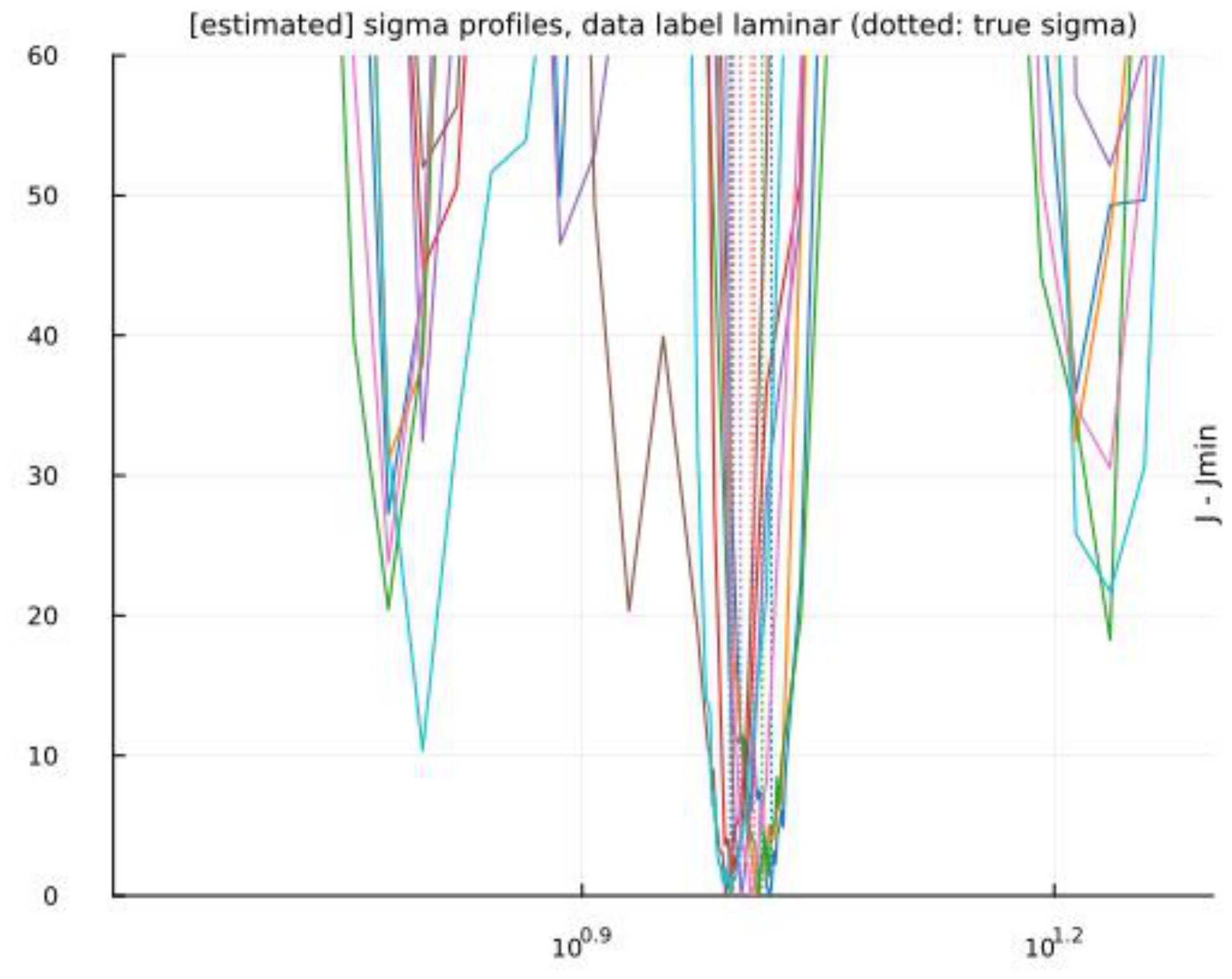
Figure 3.
b. σ-profiles by regime: chaotic, with flat multi-basin floors.
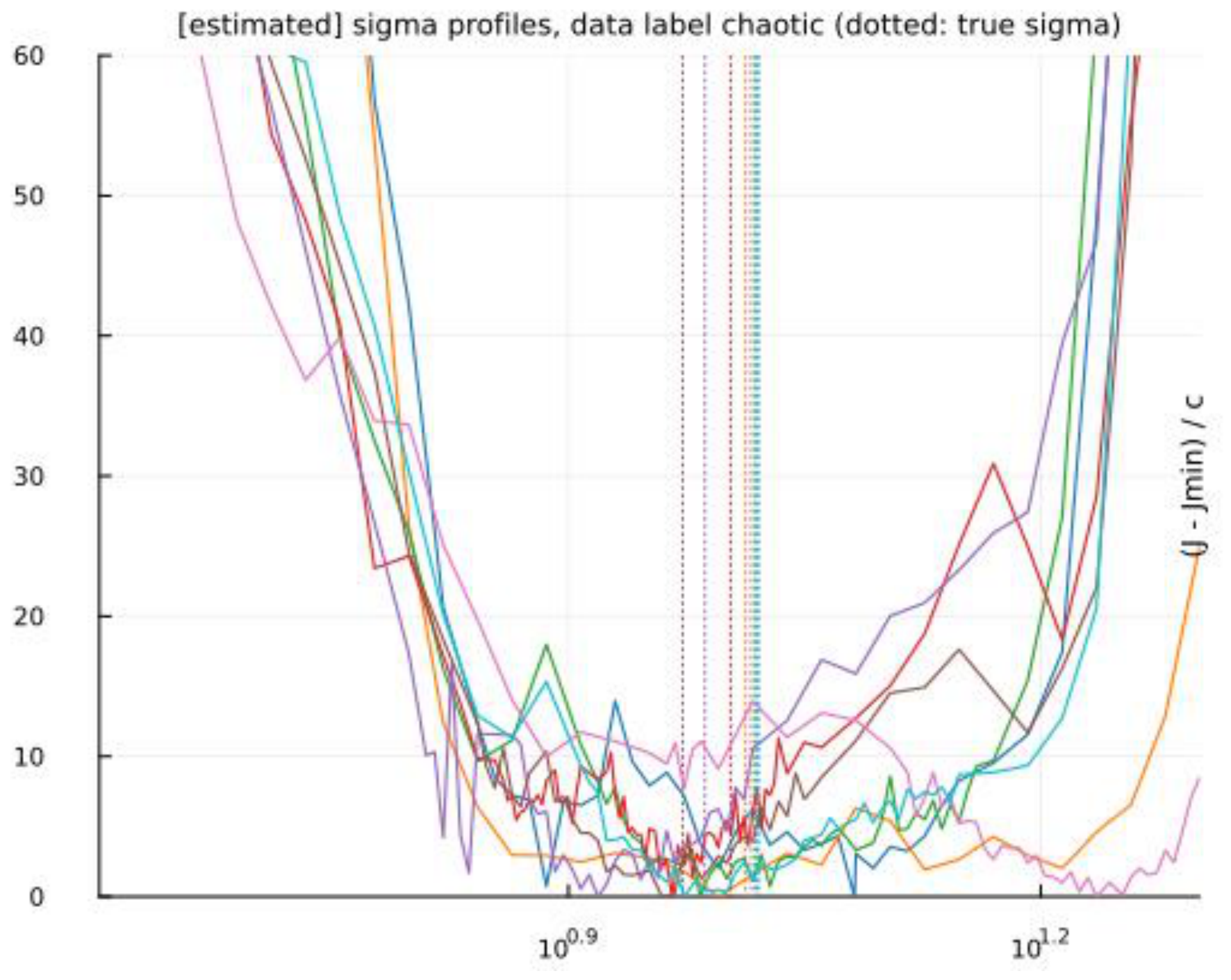
Figure 3.
c. σ-profiles by regime:laminar profiles divided by c ̂ with the 3.84 line.
3.7. Feature-Scale Model Evaluation and Virtual Populations
Both mixture models pass all six pooled features; the single-Gaussian negative control fails three, as it should. Stratified by component (8 observed subjects each, 12 tests per model), M2 flags SD z in the chaotic stratum (observed 7.46 vs PI [7.07, 7.42]) and M2T flags the half-period ACF in the chaotic stratum (observed −0.503 vs PI [−0.482, −0.360], observed percentile 0.00); the other 22 stratified tests pass, including the half-period ACF in the periodic stratum under both models. In version 3 of the pipeline, with lags fixed at 25 samples, the ACF feature was flagged in three of four stratified tests with opposite signs in the two strata; period scaling has removed the periodic-stratum flags and left a single chaotic-stratum discrepancy with a definite sign — the observed chaotic subjects are more anti-correlated at half a period (deeper, more regular troughs) than the virtual chaotic population — that reappears in the peak-aligned VPC (Section 3.8). Individual predictive checks gave median mean |z| of 0.67 (periodic) and 0.78 (chaotic) against an adequacy benchmark of ≈ 0.8; no subject had any feature beyond |z| = 3 (largest 2.56).
Regime composition of virtual populations. Of 80 subjects simulated from the single-Gaussian model, 31% settled to a fixed point — probability mass placed between the two modes where no real subjects exist. The mixture placed no mass there (0% fixed point). The untruncated mixture M2 does not reproduce the 50/50 regime split: 22.5% of draws from the periodic component fall outside the periodic window (39% periodic overall), because the window is narrow relative to the fitted and the two-component Gaussian cannot represent its edges — the same property of the generating design that rejected five of thirteen periodic candidates. The regime-truncated variant M2T, which draws the component once per virtual subject and redraws within it until it is regime-consistent, reproduced the split (45% periodic, 36/80, consistent with = 0.500 under binomial sampling; 1.17 draws per accepted periodic subject; no subject dropped). M2T is therefore the population model used for the observation-scale VPCs.
Table 12.
Feature VPC: observed median vs 90% prediction interval of the median (pooled, N = 16).
| Feature | observed | M1 (single Gaussian) | M2 (mixture) | M2T (truncated mixture) |
| mean z | 82.0 | [22.4, 146.5] | [23.5, 145.7] | [23.3, 145.4] |
| SD z | 10.17 | [3.6, 12.4] | [7.3, 13.5] | [7.3, 13.4] |
| mean peak | 99.9 | [24.1, 174.6] | [36.4, 166.3] | [36.0, 165.4] |
| CV of peaks | 0.117 | [0.052, 0.108] | [0.088, 0.211] | [0.085, 0.202] |
| mean inter-peak interval | 0.632 | [0.633, 0.833] | [0.573, 0.704] | [0.553, 0.710] |
| ACF at 0.5 P | −0.569 | [−0.274, −0.116] | [−0.591, −0.486] | [−0.597, −0.465] |
3.8. Observation-Scale VPCs
All 15 percentile checks pass. In the periodic stratum, the observed percentiles coincide with the simulated medians to the third decimal; in the chaotic stratum, the observed 5th–50th percentiles sit 0.013–0.021 log units below the simulated medians (within their intervals), a first hint that the observed chaotic subjects spend slightly more time at low than the virtual ones.
Table 13.
Marginal-quantile VPC of log y (M2T; 300 replicate populations).
| Stratum | Percentile | observed | sim median | 90% PI | flag |
|---|---|---|---|---|---|
| periodic (n = 8 vs 36 virtual) | 5 | 4.506 | 4.510 | [4.491, 4.526] | – |
| 25 | 4.786 | 4.788 | [4.771, 4.803] | – | |
| 50 | 4.991 | 4.993 | [4.978, 5.004] | – | |
| 75 | 5.185 | 5.187 | [5.175, 5.200] | – | |
| 95 | 5.452 | 5.452 | [5.440, 5.464] | – | |
| chaotic (n = 8 vs 44 virtual) | 5 | 2.295 | 2.308 | [2.272, 2.347] | – |
| 25 | 2.772 | 2.793 | [2.766, 2.826] | – | |
| 50 | 3.102 | 3.117 | [3.094, 3.144] | – | |
| 75 | 3.419 | 3.418 | [3.396, 3.441] | – | |
| 95 | 3.760 | 3.753 | [3.731, 3.774] | – | |
| pooled (n = 16 vs 80 virtual) | 5 | 2.476 | 2.470 | [2.380, 2.618] | – |
| 25 | 3.102 | 3.059 | [2.902, 3.476] | – | |
| 50 | 4.144 | 3.624 | [3.310, 4.805] | – | |
| 75 | 4.991 | 4.942 | [4.189, 5.089] | – | |
| 95 | 5.357 | 5.338 | [5.233, 5.399] | – |
Table 14.
Peak-aligned VPC (M2T): points outside their 90% prediction interval, 3 percentiles × 121 offsets.
Table 14.
Peak-aligned VPC (M2T): points outside their 90% prediction interval, 3 percentiles × 121 offsets.
| Stratum | Observed peak windows | Outside / total | % ᵃ | By τ band ᵇ |
|---|---|---|---|---|
| periodic | 576 | 33 / 363 | 9.1 | 12 / 12 / 9 |
| chaotic | 431 | 74 / 363 | 20.4 | 17 / 29 / 28 |
| pooled | 1007 | 2 / 363 | 0.6 | 0 / 1 / 1 |
ᵃ Nominal 10%. ᵇ Counts by |τ|: < 0.2 / 0.2–0.4 / > 0.4.
In the periodic stratum, the exceedance rate is at nominal, and the exceedances are spread over the whole window (the three offset bands contain 117, 120 and 126 points), so there is no evidence of peak-height misfit (which would cluster at τ ≈ 0) or inter-peak-interval misfit (which would cluster at |τ| ≈ 0.3–0.6). The chaotic stratum is different: twice the nominal exceedance, with a clear pattern. In the inter-peak shoulders (|τ| 0.25–0.5) the observed median and 95th percentile lie below their intervals at 38 of the 74 points — the observed series stay lower between peaks than the virtual series do — while within ±0.15 of the peak, the observed 5th percentile lies above its interval at 11 points — the smallest observed peaks are taller than the smallest virtual peaks. Read together with the feature VPC (half-period ACF more negative than predicted; observed inter-peak interval 0.726 at the 81st percentile of the virtual distribution), the two diagnostics agree: the virtual chaotic population oscillates slightly faster, with shallower troughs and more small peaks, than the eight observed chaotic subjects. Whether this is a deficiency of the population model (the hyper-distribution, learned from the periodic subjects, is centered at 10.04 with SD 0.017, whereas the chaotic subjects’ realized mean and SD are 10.14 and 0.041) or sampling variability of eight subjects cannot be settled at N = 16; it is reported as a residual misfit of the chaotic subpopulation.
The pooled stratum illustrates why stratification is essential. Its 90% prediction interval for the median spans 3.3–4.8 log units at every offset, because the pooled median depends on how many of the 16 resampled virtual subjects happen to be periodic; no observed percentile can fall outside such an interval, and the 0.6% exceedance is a sign of an uninformative check, not of a good model. This is the analog of a VPC pooled across two dose groups without prediction correction, and the reason the stratified panels of Figure 4 are the ones to read.
3.9. Oracle Comparison
Both arms place the realized inside the 95% credible interval, but the estimated arm fails the EBE coverage threshold (11 < 12) and the oracle arm does not, so the automated rule returns verdict A, “under-covering EBEs only with estimated noise → residual-error misestimation”. We do not accept the rule’s mechanistic reading: differs from the truth by 0.4%, far too little to change the profiles. The oracle arm’s higher (0.021 vs 0.017) and coverage come from a smaller laminar calibration constant (2.00 vs 2.82) and from a different set of Monte Carlo realizations in the stage-1 and calibration refits (the two arms simulate with different noise levels and therefore different random streams; the oracle stage-1 RMSE is 2.5 times larger because one chaotic subject landed at = 3.39). The difference between arms is a measure of the Monte-Carlo sensitivity of the pipeline at six calibration draws per regime, not of the cost of estimating . The verdict rule should be amended to require a material difference in before attributing a discrepancy to it.
Table 15.
Cost of estimating the residual-error model.
| Quantity | estimated RUV | true RUV (oracle) | target |
| b | 0.1992 | 0.2000 | 0.2000 |
| Stage 1 RMSE log / log / log | 0.151 / 0.007 / 0.019 | 0.134 / 0.011 / 0.049 | 0 |
| curvature-SE mean for log | 30.2 | 20.5 | 1.0 |
| , GTS-like | 0.179 | 0.157 | 0.032 |
| , final | 0.0166 | 0.0211 | 0.032 |
| laminar / chaotic | 2.82 / 2.44 | 2.00 / 2.29 | (truth-implied 3.5 / 3.5 and 3.0 / 3.3) |
| profiles with > 1 basin | 10 | 12 | 0 |
| EBE 90% coverage (all / periodic / chaotic) | 11 / 8 / 3 of 16 / 8 / 8 | 15 / 8 / 7 | 14.4 / 7.2 / 7.2 |
4. Discussion
What the run shows. On a benchmark where every standard estimation assumption is violated, the pipeline recovers the residual error to 0.4%, the mixture fraction and both subpopulations to within their credible intervals, the typical value and IIV, and the typical value; it reduces individual error five-fold relative to the two-stage estimates; and it reproduces the regime composition of the population. The conventional covariance route overestimates by 5.6-fold and its standard errors are off by a factor of 30 in . These results are stable across versions of the pipeline. What has changed with the period-scaled features is at the margins — improved markedly, fell further below the realized value, and the chaotic-stratum diagnostics now disagree with the model in a consistent, interpretable way — and these margins are where the remaining work lies.
Where the information aboutcomes from. The most important interpretive point of this version is that the population estimate of is effectively an estimate for the periodic subpopulation. The sensitivity table shows that responds to and hardly at all to ; the shrinkage table shows 93% shrinkage for chaotic subjects; and the realized spreads are 0.023 (periodic) and 0.041 (chaotic). With eight precise periodic estimates (synthetic RMSE 0.014) whose realized spread is 0.023, the information-theoretic best estimate of the periodic IIV is about , and dividing the profiles by removes a further share of the observed spread. The estimate of 0.017 [0.002, 0.042] is therefore not a failure of the calibration but a faithful summary of what the periodic subjects say; the realized population SD of 0.032 is dominated by chaotic subjects whose data are silent about . A pharmacometric reader will recognize the situation: an OMEGA estimated from the rich-data subgroup and applied to the sparse-data subgroup. The honest options are (i) to report as a periodic-subpopulation estimate, as we do here; (ii) to fit regime-specific , which would be unidentifiable for the chaotic component at N = 8 with flat profiles; or (iii) to collect more informative data for chaotic subjects (longer series, a second observed state).
Limitations. (1) is deflated (0.017 vs 0.032) for the reason just given, and its credible interval reaches the lower grid edge (0.002); the grid should be extended downward to confirm this is not an artifact. (2) EBE coverage for chaotic subjects was 3/8: their intervals are the population prior, which is learned from the periodic subjects and is too narrow for them. A model with a wider or regime-specific prior for the chaotic component would fix the coverage at the price of saying nothing about chaotic , which is the truthful position. (3) The calibration constants undershoot their truth-implied values in all four blocks (by 19–34%); with six draws per block this may be chance (probability 1/16 under independence), but a systematic cause — the generating value is itself a local minimum of a jagged , so synthetic data at may be “easier” than real data — deserves a dedicated experiment with more replicates (N_CAL_SUB, N_CAL_REP) and possibly per-subject constants. (4) The automated oracle verdict attributes the coverage difference between arms to residual-error misestimation, which the 0.4% error in cannot support; the two arms differ by Monte Carlo realization, and a replicate run with a second seed would quantify this directly. (5) The chaotic stratum shows a consistent residual misfit — 20% peak-aligned exceedance concentrated in the inter-peak shoulders, and a flagged half-period ACF — indicating that the virtual chaotic population oscillates slightly faster with shallower troughs than the observed chaotic subjects. Candidate causes are the hyper-distribution (centered 1% below the chaotic subjects’ realized mean, with a quarter of their realized spread) and the slightly inflated (0.0255 vs 0.0229); eight subjects cannot discriminate between these and sampling variability. (6) Conditioning on the EBE increased its error for chaotic subjects; the unconditioned EBEs should be used when shrinkage is high. (7) The EBE of one periodic subject (13) crossed into a chaotic band after shrinkage, although its Stage 1 estimate and truth are periodic; a regime-constrained EBE (reject or re-shrink an EBE that fails the Lyapunov check), the individual-level analog of the truncated mixture M2T, is a natural extension. (8) relies on bootstrap covariances; this is defensible because the two subpopulations are 1.7 log-units apart against an IIV of 0.02, so no plausible error in the covariance can move a subject between components. (9) The denoiser leaves structure in residuals (lag-1 autocorrelation 0.34); harmless under simulation symmetry but it rules out any likelihood-type use of those residuals. (10) N = 16 is small for a mixture; the wide credible interval on reflects this honestly.
Transferable conclusions for the pharmacometric reader. (i) When a structural model is oscillatory with possible irregular regimes, feature-matching objectives with simulation symmetry are a drop-in replacement for residual-based likelihoods, and the features can be chosen to match clinically meaningful summaries (pulse amplitude, inter-pulse interval). (ii) Features that depend on time should be expressed in units of each subject’s own period, not in absolute time; a fixed-lag autocorrelation confounds waveform with period and produced spurious VPC flags in both directions until it was period-scaled. (iii) Profiles with simulation-calibrated scaling provide usable individual-level uncertainty where $COV-type and bootstrap covariances fail, and the calibration experiment needs only simulation at one’s own estimates, so it applies to real data; its precision with six draws is limited and should be increased. (iv) When one subpopulation is uninformative about a parameter, the population IIV of that parameter is in effect an estimate for the informative subpopulation; shrinkage and sensitivity-to-calibration tables make this visible and should be read together. (v) Negative controls deserve a permanent place in reported output: the single-Gaussian fit, the covariance ladder, the weak chaos tests and the pooled VPC show precisely where the standard toolbox breaks. (vi) VPCs remain possible on the observation scale, but they must be event-aligned or marginal rather than indexed by absolute time, and they must be stratified by subpopulation; the truncated mixture M2T is the population model to simulate from when a component’s IIV extends past a regime boundary. (vii) Automated verdict rules are useful but their mechanistic labels must be checked against the magnitudes involved.
5. Conclusions
Population inference for ensembles of chaotic systems is feasible with honest uncertainty quantification, provided individual curvature is abandoned in favor of profiles, the profile scale is calibrated per dynamical regime by self-simulation, first-stage multimodality is treated as a certainty to be searched rather than an anomaly, features are expressed in the oscillator’s own time units, and the fitted model is validated dynamically as well as statistically. The pipeline retains the full pharmacometric vocabulary — IIV, RUV, mixtures, VPCs, EBEs, shrinkage, ETABAR — while replacing exactly those internal components that chaos invalidates. The remaining discrepancies in this version are concentrated in the chaotic subpopulation and are of a kind the diagnostics identify rather than conceal: the chaotic subjects’ data carry little information about , so the population IIV and the chaotic EBE intervals are effectively borrowed from the periodic subjects, and the chaotic waveform is reproduced slightly less well than the periodic one.
Glossary for the pharmacometric reader
| Term in this paper | Plain meaning | Related concept |
| Feature/summary statistic | A number computed from a series (peak height, interval, autocorrelation) | NCA metric |
| Period-scaled lag | A time lag expressed as a fraction of the subject’s own oscillation period | Sampling in units of the dosing interval |
| Simulated method of moments | Adjust parameters until simulated features match observed ones | Fitting simulated NCA metrics to observed |
| Common random numbers | Reuse the same seeds in every objective evaluation | Fixed seed in $SIMULATION |
| Profile (of J) | The objective as a function of one parameter, re-optimizing the others | PsN llp |
| Calibration constant c | How much steeper the objective is than a true −2 log L | Checking that ΔOFV = 3.84 really is a 95% limit |
| Posterior/credible interval | Probability distribution of a parameter given the data | Output of a BAYES run |
| Gibbs sampler | Iterative assign-then-update algorithm for the mixture | SAEM-style iterations for $MIXTURE |
| Oracle arm | Re-analysis with the true residual error plugged in | SSE with SIGMA fixed to truth |
| Truth-free | Uses only observed data; truth used solely in [validation] blocks | Analysis vs evaluation dataset |
| Lyapunov exponent | Rate at which nearby trajectories diverge; > 0 means chaos | No direct analog (regime check) |
| Simulation symmetry | Identical processing of observed and simulated data | Prediction correction in pcVPC |
| Marginal-quantile VPC | Percentiles of all observations in a stratum vs their simulated PI, ignoring time | VPC of the concentration distribution |
| Peak-aligned VPC | Percentiles of observations vs time since the nearest detected peak | Dose-aligned steady-state VPC |
| Truncated mixture (M2T) | Mixture whose components are restricted to their own dynamical regime | $MIXTURE with a bounded parameter per subpopulation |
Supplementary Materials
The following supporting information can be downloaded at the website of this paper posted on Preprints.org.
Funding Statement
This study received no funding.
Acknowledgments
The author utilized Claude Fable 5.1 and Claude Opus 5.5 (Anthropic) generative AI models to brainstorm, search literature, generate and debug code, condense the abstract, and help select keywords. The author conceived the study, designed and carried out the analyses, interpreted the results, and critically reviewed the whole manuscript, including the code. The author takes full responsibility for the content of this publication.
Competing interests
The author is the sole proprietor of Freedman Patent, which provides expert witness services in litigation. No part of this work was commissioned by, funded by, or carried out for any party to litigation. The author has no other relevant financial or non-financial interests to disclose.
References
- Lavielle, M. Mixed Effects Models for the Population Approach; CRC Press, 2014. [Google Scholar]
- Lindstrom, M.J.; Bates, D.M. Biometrics 1990, 46, 673–687. [PubMed]
- Keenan, D.M.; Veldhuis, J.D. Physiology 2016, 31, 34–50. [PubMed]
- Sturis, J.; Polonsky, K.S.; Mosekilde, E.; Van Cauter, E. Am. J. Physiol. 1991, 260, E801–E809. [PubMed]
- Goldbeter, A. Biochemical Oscillations and Cellular Rhythms; Cambridge University Press, 1996. [Google Scholar]
- Steimer, J.-L.; Mallet, A.; Golmard, J.-L.; Boisvieux, J.-F. Drug Metab. Rev. 1984, 15, 265–292. [PubMed]
- Lorenz, E.N. J. Atmos. Sci. 1963, 20, 130–141.
- Barrio, R.; Serrano, S. Physica D. 2007, 229, 43–51.
- Carlsson, K.C.; Savić, R.M.; Hooker, A.C.; Karlsson, M.O. AAPS J. 2009, 11, 148–154. [PubMed]
- Benettin, G.; Galgani, L.; Giorgilli, A.; Strelcyn, J.-M. Meccanica 1980, 15, 9–30.
- Donoho, D.L.; Johnstone, I.M. Biometrika 1994, 81, 425–455.
- Bergstrand, M.; Hooker, A.C.; Wallin, J.E.; Karlsson, M.O. AAPS J. 2011, 13, 143–151. [CrossRef] [PubMed]
- Bandt, C.; Pompe, B. Phys. Rev. Lett. 2002, 88, 174102. [PubMed]
- Gottwald, G.A.; Melbourne, I. Proc. R Soc. A 2004, 460, 603–611.
- McFadden, D. Econometrica 1989, 57, 995–1026.
- Gouriéroux, C.; Monfort, A. Simulation-Based Econometric Methods; OUP, 1996. [Google Scholar]
- Raue, A.; Kreutz, C.; Maiwald, T.; et al. Bioinformatics 2009, 25, 1923–1929. [CrossRef] [PubMed]
- Savić, R.M.; Karlsson, M.O. AAPS J. 2009, 11, 558–569. [PubMed]
- Dosne, A.-G.; Bergstrand, M.; Harling, K.; Karlsson, M.O. J. Pharmacokinet. Pharmacodyn. 2016, 43, 583–596. [PubMed]
Figure 1.
First 8 time units of four subjects (1, 3, 16, 15): raw log y (grey), noise-free log z (black), denoised series (color). Periodic subjects show regular peaks; chaotic subjects irregular ones. Note how the wavelet smoother flattens the sharp period.
Figure 1.
First 8 time units of four subjects (1, 3, 16, 15): raw log y (grey), noise-free log z (black), denoised series (color). Periodic subjects show regular peaks; chaotic subjects irregular ones. Note how the wavelet smoother flattens the sharp period.
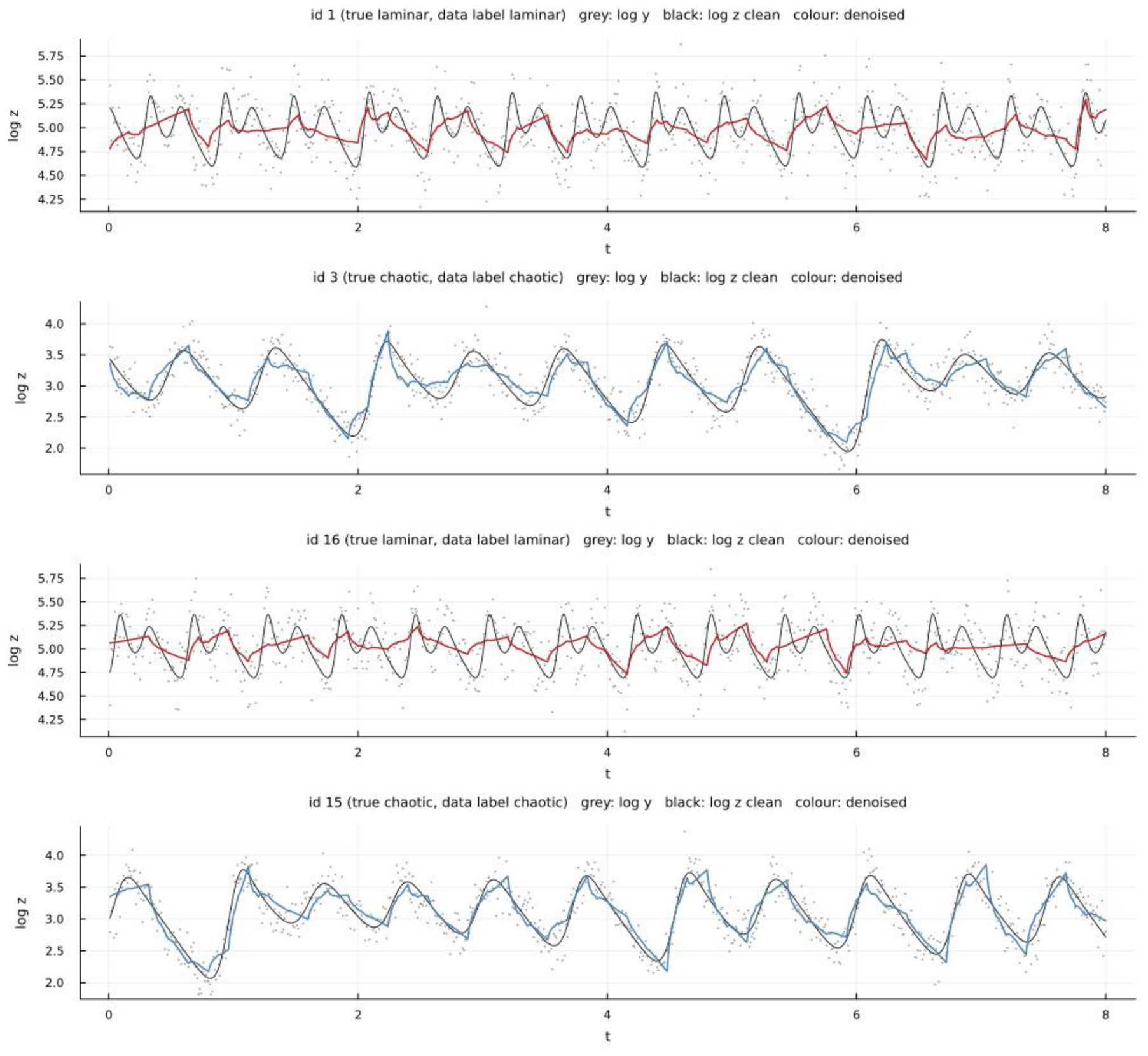
Figure 2.
Truth-free regime discriminators (left: log CV of peaks vs dominant period with the gap cuts; right: permutation entropy, colored by true regime).
Figure 2.
Truth-free regime discriminators (left: log CV of peaks vs dominant period with the gap cuts; right: permutation entropy, colored by true regime).
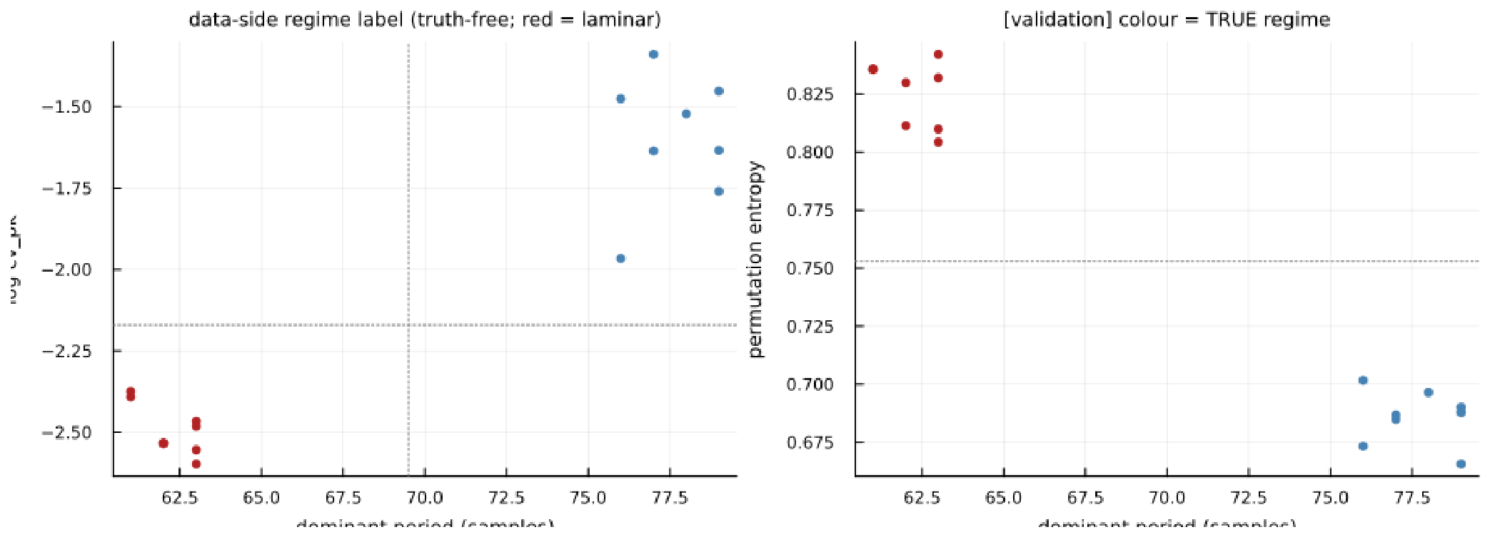
Figure 4.
Observation-scale VPCs from the M2T population, six panels: rows = periodic, chaotic, pooled strata; left column marginal-quantile VPC (observed percentiles of log y in red, 90% PI in blue); right column peak-aligned VPC (observed 5th/50th/95th percent).
Figure 4.
Observation-scale VPCs from the M2T population, six panels: rows = periodic, chaotic, pooled strata; left column marginal-quantile VPC (observed percentiles of log y in red, 90% PI in blue); right column peak-aligned VPC (observed 5th/50th/95th percent).
Disclaimer/Publisher’s Note: The statements, opinions and data contained in all publications are solely those of the individual author(s) and contributor(s) and not of MDPI and/or the editor(s). MDPI and/or the editor(s) disclaim responsibility for any injury to people or property resulting from any ideas, methods, instructions or products referred to in the content. |
© 2026 by the authors. Licensee MDPI, Basel, Switzerland. This article is an open access article distributed under the terms and conditions of the Creative Commons Attribution (CC BY) license (http://creativecommons.org/licenses/by/4.0/).
Copyright: This open access article is published under a Creative Commons CC BY 4.0 license, which permit the free download, distribution, and reuse, provided that the author and preprint are cited in any reuse.