Bivariant Hodge Atoms I: Hecke Collisions and Mixed-Hodge Coefficient Extensions

1. Introduction

The interaction between singular Hodge theory, geometric correspondences, and geometric Langlands raises a natural question: can the local specialization and extension structures associated with singular degenerations be transported compatibly through Hecke modifications and their composition? Such compatibility would provide a possible route from singular Hodge-atom constructions toward the categorical geometry underlying Hecke actions, affine Grassmannians, and ultimately geometric Langlands. A central difficulty is that conventional convolution invariants and derived direct-image decompositions do not, by themselves, determine the extension morphisms through which singular Hodge-theoretic contributions are assembled.

An important precedent is Gaitsgory’s construction of central sheaves through nearby cycles, which demonstrates that specialization can interact nontrivially with affine-Hecke convolution [1]. Together with geometric Satake and the categorical birational geometry of Grothendieck resolutions, this suggests investigating whether mixed-Hodge-module specialization and extension data admit compatible correspondence-level structures [2,3,4]. Our approach is deliberately incremental: before attempting general Hecke actions or geometric-Langlands realizations, we examine explicit finite-dimensional modification towers in which the relevant morphisms, specialization diagrams, and extension classes can be calculated and verified.

We begin with $G{L}_2$ and $G{L}_3$ Hecke collisions, constructing their canonical mixed-Hodge coefficient comparisons from proper incidence maps. The first calculation shows that isomorphic nearby-cycle objects and trivial unipotent monodromy can conceal different canonical and vanishing-cycle morphisms. The second establishes a more subtle distinction: the derived composition-defect triangle splits while all three underlying coefficient extensions remain nonsplit. These results show that any proposed correspondence-level transport of singular Hodge-theoretic structures must account for extension morphisms, not only their graded constituents or derived defect classes.

The purpose of this paper is twofold: to establish concrete mixed-Hodge models for the interaction of singular specialization data with Hecke composition, and to identify the additional structures required for a possible geometric-Langlands connection. The subsequent program asks whether these local calculations extend to higher type-A modifications, global Springer-orbit gluing, coherent Hecke realizations, and ultimately Hecke–Hitchin correspondences. No geometric-Langlands equivalence or general Hecke action is asserted here; rather, the present results supply the first explicitly verified comparison structures toward investigating those possibilities.

1.1. Motivation

The Hodge-theoretic constituents of a degeneration do not, in general, determine the morphisms through which they are assembled. Nearby and vanishing cycles, monodromy, canonical and variation morphisms, and extension classes contain information not recovered from cohomological dimensions or Grothendieck-group identities. This distinction is fundamental to limiting mixed Hodge theory [5,6,7,8,9], perverse gluing [10,11], and Saito’s theory of mixed Hodge modules [12,13].

The Hodge-atom program of Katzarkov–Kontsevich–Pantev–Yu relates Hodge-theoretic structures to non-archimedean F-bundles associated with quantum multiplication and the Euler field [14]. Its equivariant developments motivate the study of symmetry and representation – theoretic structures on atomic constituents [15,16].

The author’s singular Hodge-atom program develops the degeneration-theoretic direction through perverse nearby and vanishing cycles, corrected extensions, limiting mixed Hodge modules, and rigid–flexible decompositions at conifold singularities [17,18,19]. The Stokes–extension constructions retain the morphisms attaching local singular contributions to ambient intersection-complex sectors. Global cycle relations and equivariant gluing constrain their assembly in multi-node degenerations [20,21,22].

These developments motivate the question addressed here: how do mixed-Hodge coefficient extensions behave under composition of geometric modification correspondences? Hecke modifications provide a natural setting. Their convolution geometry has finite-dimensional Schubert, Quot, and invariant-flag models, while geometric Satake supplies its representation-theoretic interpretation [2,3,23,24]. Forgetting intermediate modifications defines proper maps whose adjunction units compare mixed-Hodge-module coefficients on a common terminal space.

We calculate these comparisons in a two-step $G{L}_2$ collision and a transverse three-step $G{L}_3$ collision. The first yields two coefficients with isomorphic nearby cycles and trivial unipotent monodromy, but different canonical maps and a nonsplit coefficient extension. The second yields a split octahedral composition-defect triangle although all three coefficient extensions are nonsplit.

The calculations use the actual incidence maps, proper base change, small and semismall resolutions, Saito specialization, and derived Hom groups [13,25]. They are bivariant in the restricted sense that the coefficient comparisons are attached to geometric morphisms and their composition, rather than constituting a full Fulton–MacPherson bivariant theory [26,27].

1.2. The Rank-One Question and Its Geometric Boundaries

We begin with $G=G{L}_2$, $\mathcal{O}=\mathbb{C}\left[\right[z\left]\right]$, $\mathcal{K}=\mathbb{C}\left(\right(z\left)\right)$, and ${\mathrm{\Lambda }}_0={\mathcal{O}}^2$. For $\mu =(1,0)$, the minuscule Schubert variety is $S_{\mu }\simeq {\mathbb{P}}^1$, and its two-step convolution resolution is

$$\tilde{S}=S_{\mu }\tilde{\times }{S}_{\mu }\simeq {\mathbb{F}}_2,m_0:\tilde{S}⟶S_{(2,0)}.$$

(1)

The negative section contracts to the $A_1$ singularity of $S_{(2,0)}$ [2,3].

For modifications supported at $z=0,s$, multiplication by z on a framed terminal quotient has matrix

$$A=\left(\begin{array}{cc}a& b\\ c& s-a\end{array}\right),a(s-a)-bc=0.$$

(2)

Putting $x=a$ and $y=s-a$ gives the relative terminal threefold $\mathcal{S}=\{xy-bc=0\}$ with $f=x+y$. Its central fiber $S=\{x^2+bc=0\}$ is an $A_1$ surface singularity, and the relative small resolution $m_B:\tilde{\mathcal{S}}\to \mathcal{S}$ has smooth source.

The resolved central fiber is $Tot\left({\mathcal{O}}_{{\mathbb{P}}^1}(-2)\right)$, not the entire projective convolution surface ${\mathbb{F}}_2$. The equation ${\left(x-{\displaystyle \frac{s}{2}}\right)}^2+bc={\displaystyle \frac{s^2}{4}}$ also exhibits the quadratic Weyl-base-change structure of the $A_1$ simultaneous resolution [28,29].

Let ${\mathbf{1}}_Y^H$ denote the derived constant Hodge complex. The relative resolution supplies

$$\mathcal{M}={\mathbf{1}}_{\mathcal{S}}^H\left[3\right],\mathcal{N}=R{m}_{B*}{\mathbf{1}}_{\tilde{\mathcal{S}}}^H\left[3\right],\eta :\mathcal{M}⟶\mathcal{N}.$$

(3)

Writing $k_p:\left\{p\right\}\hookrightarrow \mathcal{S}$ for the exceptional point, the comparison has $\mathrm{Cone}\left(\eta \right)\simeq k_{p*}{\mathbb{Q}}_p^H(-1)\left[1\right]$, and yields a nonsplit short exact sequence in $\mathrm{MHM}\left(\mathcal{S}\right)$:

$$0⟶k_{p*}{\mathbb{Q}}_p^H(-1)⟶\mathcal{M}\stackrel{\eta }{\to }\mathcal{N}⟶0.$$

Its nonsplitting follows from the vanishing ${Hom}_{{\mathsf{D}}_H\left(\mathcal{S}\right)}(\mathcal{M},k_{p*}{\mathbb{Q}}_p^H(-1))=0$.

For normalized unipotent nearby and vanishing cycles ${\mathrm{\Psi }}_f^H,{\mathrm{\Phi }}_f^H$, define

$$P_f^H\left(\mathcal{L}\right)=\mathrm{Cone}\left({\mathrm{Var}}_{\mathcal{L}}:{\mathrm{\Phi }}_f^H\mathcal{L}⟶{\mathrm{\Psi }}_f^H\mathcal{L}(-1)\right)[-1].$$

(4)

The variation triangle gives $P_f^H\left(\mathcal{L}\right)\simeq i^{!}\mathcal{L}$, where $i:S\hookrightarrow \mathcal{S}$. The associated comparison defect is

$${\mathfrak{D}}_f\left(\eta \right)=\mathrm{Cone}\left(P_f^H\left(\eta \right):P_f^H\left(\mathcal{M}\right)⟶P_f^H\left(\mathcal{N}\right)\right).$$

(5)

Thus ${\mathfrak{D}}_f\left(\eta \right)\simeq i^{!}\mathrm{Cone}\left(\eta \right)$. Its specialization package also retains the canonical, variation, and monodromy maps [11,13].

For three ordered modifications at $z=0,s,2s$, the relevant geometry is the $G{L}_3$ invariant-flag tower

$${\mathcal{X}}_2\stackrel{r}{\to }{\mathcal{X}}_1\stackrel{q}{\to }{\mathcal{X}}_0.$$

(6)

It is the Grothendieck–Springer construction restricted to the ordered eigenvalue line $(0,s,2s)$. Near a subregular nilpotent matrix, its transverse model is

$$\mathcal{T}:xy=w(w-s)(w+s).$$

(7)

The central fiber $xy=w^3$ is of type $A_2$, and the family is the restriction $(\alpha ,\beta )=(-s^2,0)$ of $xy=w^3+\alpha w+\beta$ [29].

Its two successive incidence resolutions have composite exceptional fiber $E=E_1\cup E_2$, where $E_1,E_2\simeq {\mathbb{P}}^1$ meet at one point and $H^2(E,\mathbb{Q})\simeq \mathbb{Q}{(-1)}^{\oplus 2}$. Section 5 identifies the incidence maps with the transverse restrictions of the ordered forgetful maps, using explicit kernel-line equations. This construction lies within the broader type-A matrix-slice framework [30].

The global family has dimension seven and coefficient normalization $\left[7\right]$; the transverse threefold uses $\left[3\right]$. The global zero nilpotent orbit contributes additional Springer-fiber geometry, so the point-supported transverse calculation does not determine the complete global composition obstruction.

1.3. Review of the Literature

Perverse gluing and mixed Hodge modules provide the foundational specialization formalism [10,11,12,13]. The present problem concerns the actual adjunction morphisms and extension classes produced by finite-dimensional modification geometry, rather than a new construction of these functors.

The comparison between the shifted constant Hodge complex and the intersection Hodge module has a substantial antecedent in the theory of singular Hodge-module defects. In particular, Park and Popa study the canonical comparison triangle ${\mathcal{K}}_X^{•}\to {\mathbf{1}}_X^H\left[n\right]\to {\mathrm{IC}}_X^H\stackrel{+1}{\to }$ and its relation to rational homology manifold properties [31]. The two-step coefficient sequence of Proposition 14 is an explicit determinantal instance of this constant-to-intersection comparison: its point-supported contribution is $k_{p*}{\mathbb{Q}}_p^H(-1)$. Our use of the comparison is distinguished by the geometrically specified Hecke adjunction map, its full specialization diagram, and its role in subsequent ordered composition calculations.

The relationship between nearby cycles and Springer geometry is likewise classical. Grinberg develops nearby-cycle constructions associated with the adjoint quotient and generalizations of Springer theory [32]. Brieskorn–Slodowy simultaneous-resolution geometry and its Weyl-monodromy interpretation also admit extensions to mixed characteristic [29,33]. The present paper does not introduce this geometry or its monodromy formalism. Instead, it identifies the ordered finite-dimensional forgetful maps with their transverse incidence models and computes the resulting mixed-Hodge coefficient morphisms.

A closely related categorical perspective appears in the work of Bondal–Kapranov– Schechtman on perverse schobers and birational geometry [4]. Their treatment of flop diagrams and Grothendieck resolutions, including the ${\mathfrak{sl}}_3$ case, provides an important predecessor for organizing birational correspondences categorically. Our construction has a different target: it works with specified objects and morphisms in derived mixed-Hodge-module categories, retaining their nearby- and vanishing-cycle maps, adjunction cones, and Yoneda extensions. In particular, it is not a numerical decategorification of the schober formalism, nor does it construct a schober on the Hecke correspondence category.

Geometric Satake interprets affine-Grassmannian convolution through representations [2,3,23]. The three-step geometry is related to the Grothendieck–Springer resolution, the Brieskorn–Slodowy deformation, and type-A matrix-slice correspondences [29,30]. The author’s earlier conifold constructions provide a related, but geometrically distinct, source of perverse-extension and composition data. The perverse-schober treatment of a single ordinary double point constructs a corrected perverse carrier using variation and the nearby–vanishing-cycle formalism [34]. The intersection-space Hodge-atom construction further organizes singular contributions through defect triangles and comparisons with intersection-complex data [35].

These developments motivate retaining extension morphisms rather than only their graded constituents. The present paper introduces a different geometric source for those morphisms: the adjunction units of ordered Hecke modification towers. Its principal new calculation is the simultaneous splitting of the transverse composition-defect triangle and nonsplitting of the three underlying coefficient extensions, as established in Theorem 3. No identification with a particular rigid–flexible Hodge-atom carrier is assumed.

Nearby-cycle methods also enter affine-Hecke theory through Gaitsgory’s central-sheaf construction and higher nearby cycles [1,36]. Our objects are different: they are adjunction comparisons between coefficients on a finite-type terminal modification space. Their cones, specialization diagrams, and Yoneda classes constitute the invariants calculated here.

Constructible–coherent affine-Hecke methods, graded Hodge modules, and coherent singular support offer potential settings for transporting these extension data [37,38,39]. The Hitchin fibration, global Springer theory, and the gauge-theoretic interpretation of line operators provide further motivation [40,41,42,43]. These connections are not required for the proofs below.

1.4. Organization of the Paper

Section 3 constructs the $G{L}_2$ convolution surface and the affine collision resolution. The projective semismall decomposition is

$$R{m}_{0*}{\mathbf{1}}_{\tilde{S}}^H\left[2\right]\simeq {\mathrm{IC}}_{S_{(2,0)}}^H\oplus i_{p*}{\mathbb{Q}}_p^H(-1).$$

This pure decomposition is distinguished from the relative coefficient extension on $\mathcal{S}$.

Section 4 computes the full specialization data of (3). Writing $I={\mathrm{IC}}_S^H$ and $T=j_{p*}{\mathbb{Q}}_p^H(-1)$, Theorem 2 establishes ${\mathrm{\Psi }}_f^H\mathcal{M}\simeq {\mathrm{\Psi }}_f^H\mathcal{N}\simeq I\oplus T$, but ${\mathrm{\Phi }}_f^H\mathcal{M}\simeq T$ and ${\mathrm{\Phi }}_f^H\mathcal{N}=0$. Moreover, ${\mathrm{can}}_{\mathcal{M}}={pr}_T$, ${\mathrm{Var}}_{\mathcal{M}}=0$, and $N_{\mathcal{M}}=N_{\mathcal{N}}=0$. Proposition 15 proves that the coefficient extension is nonsplit.

Section 5 constructs the $G{L}_3$ invariant-flag tower and its transverse $A_2$ incidence model. For the global seven-dimensional family, the coefficient objects are

$$\begin{array}{cc}\hfill {\mathcal{A}}_0& ={\mathbf{1}}_{{\mathcal{X}}_0}^H\left[7\right],\hfill \\ \hfill {\mathcal{A}}_1& =R{q}_{*}{\mathbf{1}}_{{\mathcal{X}}_1}^H\left[7\right],\hfill \\ \hfill {\mathcal{A}}_2& =R{\left(qr\right)}_{*}{\mathbf{1}}_{{\mathcal{X}}_2}^H\left[7\right].\hfill \end{array}$$

(8)

Their adjunction comparisons induce

$${\mathfrak{D}}_u⟶{\mathfrak{D}}_{vu}⟶{\mathfrak{D}}_v\stackrel{{\omega }_{q,r}^H}{\to }{\mathfrak{D}}_u\left[1\right].$$

(9)

Section 6 calculates this construction on the transverse threefold, with shift $\left[3\right]$. For $T_p=k_{p*}{\mathbb{Q}}_p^H(-1)$, the three coefficient comparison cones are $T_p\left[1\right]$, $T_p\left[1\right]$, and $T_p^{\oplus 2}\left[1\right]$. The local connecting morphism vanishes because ${Ext}_{\mathrm{MHS}}^1(\mathbb{Q}(-1),\mathbb{Q}(-1))=0$, while all three coefficient sequences are nonsplit. This is Theorem 3.

Section 7 relates these results to singular Hodge-atom extension data. Section 8 discusses higher type-A towers, global Springer-orbit gluing, coherent realizations, and Hecke–Hitchin comparisons. The general-n theorem and global obstruction calculation remain open problems in this paper.

2. Categories, Conventions, and Hypotheses

We fix the mixed-Hodge-module conventions and geometric hypotheses used throughout. The underlying formalism is due to Saito [12,13].

2.1. Derived Categories of Mixed Hodge Modules

All varieties are of finite type over $\mathbb{C}$, with rational coefficients.

Definition 1.

For a complex algebraic variety Y, let $\mathrm{MHM}\left(Y\right)$ be Saito’s abelian category of mixed Hodge modules, and put ${\mathsf{D}}_H\left(Y\right)=D^b\mathrm{MHM}\left(Y\right)$. Write ${\mathcal{H}}_H^k$ for its standard cohomology functors and

$${Hom}_{H,Y}(K,L)={Hom}_{{\mathsf{D}}_H\left(Y\right)}(K,L),{Ext}_{H,Y}^k(K,L)={Hom}_{H,Y}(K,L\left[k\right]).$$

For heart objects, ${Ext}_{H,Y}^1$ agrees with Yoneda ${Ext}^1$.

The realization functor ${\mathrm{rat}}_Y:{\mathsf{D}}_H\left(Y\right)\to D_c^b(Y,\mathbb{Q})$ commutes with the relevant six operations and specialization. Its restriction $\mathrm{MHM}\left(Y\right)\to \mathrm{Perv}(Y,\mathbb{Q})$ is exact and faithful [13].

Definition 2.

Let $a_Y:Y\to Spec\mathbb{C}$ be the structural morphism. Define ${\mathbf{1}}_Y^H=a_Y^{*}{\mathbb{Q}}_{\mathrm{pt}}^H$.

If Y is smooth of dimension d, ${\mathbf{1}}_Y^H\left[d\right]\in \mathrm{MHM}\left(Y\right)$. For irreducible Y of dimension d with smooth dense open $j:U\hookrightarrow Y$, put ${\mathrm{IC}}_Y^H=j_{!*}{\mathbf{1}}_U^H\left[d\right]$. For reducible pure-dimensional Y, take the sum over irreducible components.

Remark 1.

On singular Y, the shifted constant complex need not be perverse or coincide with ${\mathrm{IC}}_Y^H$. The necessary heart concentration is established for the collision models where it is used.

We use the Tate convention $wt\mathbb{Q}\left(m\right)=-2m$. In particular, $\mathbb{Q}(-1)$ has weight two. For proper g, one has $g_{!}=g_{*}$.

Definition 3.

For $K\in {\mathsf{D}}_H\left(Y\right)$, put ${amp}_H\left(K\right)=\{k:{\mathcal{H}}_H^k\left(K\right)\ne 0\}$. Then $K\in \mathrm{MHM}\left(Y\right)$ precisely when ${amp}_H\left(K\right)\subseteq \left\{0\right\}$.

Remark 2.

Cones are formed in ${\mathsf{D}}_H\left(Y\right)$. A heart-level short exact sequence and its Yoneda class require the corresponding cohomological concentration.

2.2. Nearby Cycles, Vanishing Cycles, and Morphisms

Let $f:X\to B$ be a morphism to a smooth curve, with distinguished fiber $X_0=f^{-1}\left(0\right)$ and $i:X_0\hookrightarrow X$.

Definition 4.

For unshifted unipotent nearby and vanishing cycles ${\psi }_{f,1}^H$ and ${\varphi }_{f,1}^H$, set ${\mathrm{\Psi }}_f^H={\psi }_{f,1}^H[-1]$ and ${\mathrm{\Phi }}_f^H={\varphi }_{f,1}^H[-1]$. These functors are t-exact on $\mathrm{MHM}\left(X\right)$ and extend to ${\mathsf{D}}_H\left(X\right)\to {\mathsf{D}}_H\left(X_0\right)$.

Unless indicated otherwise, the eigenvalue-one summand is understood. We use the logarithmic normalization $N={\left(2\pi i\right)}^{-1}\log T_u$, with the corresponding Tate-twisted variation map [13].

Definition 5.

For $\mathcal{L}\in {\mathsf{D}}_H\left(X\right)$, write

$${\mathrm{sp}}_{\mathcal{L}}:i^{*}\mathcal{L}[-1]\to {\mathrm{\Psi }}_f^H\mathcal{L},{\mathrm{can}}_{\mathcal{L}}:{\mathrm{\Psi }}_f^H\mathcal{L}\to {\mathrm{\Phi }}_f^H\mathcal{L},$$

and ${\mathrm{Var}}_{\mathcal{L}}:{\mathrm{\Phi }}_f^H\mathcal{L}\to {\mathrm{\Psi }}_f^H\mathcal{L}(-1)$. The convention satisfies $N_{\mathcal{L}}={\mathrm{Var}}_{\mathcal{L}}\circ {\mathrm{can}}_{\mathcal{L}}$.

Proposition 1.

For every $\mathcal{L}\in {\mathsf{D}}_H\left(X\right)$, there are functorial distinguished triangles

$$i^{*}\mathcal{L}[-1]\stackrel{{\mathrm{sp}}_{\mathcal{L}}}{\to }{\mathrm{\Psi }}_f^H\mathcal{L}\stackrel{{\mathrm{can}}_{\mathcal{L}}}{\to }{\mathrm{\Phi }}_f^H\mathcal{L}\stackrel{+1}{\to }$$

and

$${\mathrm{\Phi }}_f^H\mathcal{L}\stackrel{{\mathrm{Var}}_{\mathcal{L}}}{\to }{\mathrm{\Psi }}_f^H\mathcal{L}(-1)⟶i^{!}\mathcal{L}\left[1\right]\stackrel{+1}{\to }.$$

These are compatible with rational realization and proper direct image [13].

Proof. 

These are Saito’s normalized unipotent specialization and variation triangles. □

Definition 6.

Define

$$P_f^H\left(\mathcal{L}\right)=\mathrm{Cone}\left({\mathrm{Var}}_{\mathcal{L}}:{\mathrm{\Phi }}_f^H\mathcal{L}\to {\mathrm{\Psi }}_f^H\mathcal{L}(-1)\right)[-1].$$

For composable morphisms, we use compatible cofibers in a fixed derived enhancement.

Proposition 2.

There is a functorial isomorphism $P_f^H\left(\mathcal{L}\right)\simeq i^{!}\mathcal{L}$.

Proof. 

The variation triangle identifies $\mathrm{Cone}\left({\mathrm{Var}}_{\mathcal{L}}\right)$ with $i^{!}\mathcal{L}\left[1\right]$. □

Corollary 1.

The variation cone belongs to $\mathrm{MHM}\left(X_0\right)$ if and only if ${\mathcal{H}}_H^k\left(i^{!}\mathcal{L}\right)=0$ for all $k\ne 0$.

Proof. 

Apply standard cohomology to Proposition 2. □

Remark 3.

The variation cone is a derived object, not automatically a coefficient extension in the perverse heart.

Proposition 3.

For $\mathcal{L}\in {\mathsf{D}}_H\left(X\right)$, the variation triangle gives

$$\begin{array}{cc}\hfill \dots \to & {\mathcal{H}}_H^{k-1}\left({\mathrm{\Psi }}_f^H\mathcal{L}(-1)\right)\to {\mathcal{H}}_H^k\left(P_f^H\left(\mathcal{L}\right)\right)\hfill \\ \hfill \to & {\mathcal{H}}_H^k\left({\mathrm{\Phi }}_f^H\mathcal{L}\right)\to {\mathcal{H}}_H^k\left({\mathrm{\Psi }}_f^H\mathcal{L}(-1)\right)\to \dots .\hfill \end{array}$$

If $\mathcal{L}\in \mathrm{MHM}\left(X\right)$, the only possibly nonzero cohomology objects are

$${\mathcal{H}}_H^0\left(P_f^H\left(\mathcal{L}\right)\right)\simeq \ker \left({\mathrm{Var}}_{\mathcal{L}}\right),{\mathcal{H}}_H^1\left(P_f^H\left(\mathcal{L}\right)\right)\simeq coker\left({\mathrm{Var}}_{\mathcal{L}}\right).$$

Proof. 

The normalized cycle functors are t-exact. Applying standard cohomology to $P_f^H\left(\mathcal{L}\right)\to {\mathrm{\Phi }}_f^H\mathcal{L}\stackrel{{\mathrm{Var}}_{\mathcal{L}}}{\to }{\mathrm{\Psi }}_f^H\mathcal{L}(-1)\stackrel{+1}{\to }$ gives the stated sequence and, for $\mathcal{L}$ in the heart, its kernel and cokernel. □

Corollary 2.

For $\mathcal{L}\in \mathrm{MHM}\left(X\right)$, $P_f^H\left(\mathcal{L}\right)\in \mathrm{MHM}\left(X_0\right)$ if and only if ${\mathrm{Var}}_{\mathcal{L}}$ is an epimorphism. In that case, $P_f^H\left(\mathcal{L}\right)\simeq \ker \left({\mathrm{Var}}_{\mathcal{L}}\right)$.

Proof. 

By Proposition 3, heart concentration is equivalent to the vanishing of the cokernel. □

Remark 4.

Nonunipotent eigenvalues have the corresponding canonical and variation conventions. The calculations below use the unipotent summand.

2.3. Admissible Geometric and Categorical Data

The explicit modification models are specified in Section 3 and Section 5. We use their incidence presentations to establish the required properness and smoothness.

Definition 7.

A bounded modification datum consists of a smooth complex curve C, a parameter curve B, a vector bundle $\mathcal{E}$ on $C\times B$, and bounded quotient conditions defining terminal and chain spaces $Q,F$ over B, with a forgetful morphism $\pi :F\to Q$.

Definition 8.

A modification datum is admissible for a specified result when its required properties have been verified: finite-type representation of the incidence functors, properness of the forgetful maps, the asserted smoothness properties, applicability of proper base change and specialization, and any perverse or equivariant descent statements invoked.

Specialization always follows Section 2.2.

Remark 5.

The relevant forgetful maps are projective because the incidence conditions define closed subschemes of products with projective Grassmannian or flag varieties.

Remark 6.

Smoothness of the source need not imply smoothness over B. For the two-step resolved family, relative smoothness is verified in Proposition 12.

Consider a Cartesian square

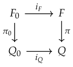
where $\pi$ is proper over B and the structural maps satisfy $g\pi =f$.

Proposition 4.

For $\mathcal{L}\in {\mathsf{D}}_H\left(F\right)$, proper base change and specialization give

$$i_Q^{*}{\pi }_{*}\mathcal{L}\simeq {\pi }_{0*}{i}_F^{*}\mathcal{L},i_Q^{!}{\pi }_{*}\mathcal{L}\simeq {\pi }_{0*}{i}_F^{!}\mathcal{L},$$

and

$${\mathrm{\Psi }}_g^H\left({\pi }_{*}\mathcal{L}\right)\simeq {\pi }_{0*}{\mathrm{\Psi }}_f^H\mathcal{L},{\mathrm{\Phi }}_g^H\left({\pi }_{*}\mathcal{L}\right)\simeq {\pi }_{0*}{\mathrm{\Phi }}_f^H\mathcal{L}.$$

These identifications preserve specialization, canonical and variation maps, monodromy, and Tate twists [13].

Proof. 

The first two are proper base-change isomorphisms. Nearby cycles commute with proper direct image, and naturality of the specialization and variation triangles gives the remaining compatibilities. □

Corollary 3.

Under the preceding hypotheses, $P_g^H\left({\pi }_{*}\mathcal{L}\right)\simeq {\pi }_{0*}{P}_f^H\left(\mathcal{L}\right)$.

Proof. 

Use $P^H\simeq i^{!}$ and extraordinary proper base change. □

Remark 7.

These are derived-category identifications. Proper direct image is not generally perverse t-exact.

Definition 9.

A categorical realization comprises the coefficient objects and adjunction comparisons induced by the specified geometric maps. An equivariant realization additionally includes the required equivariant descent data.

Remark 8.

A finite-dimensional Quot–Schubert identification alone does not establish equivariant Satake convolution. Positive-loop-group descent is required [2,3].

Remark 9.

The incidence spaces and adjunction comparisons are constructed first; their coefficient cones and extension classes are then calculated from those geometric maps.

Remark 10.

Heart concentration and nonsplitting in the explicit local models are established by the coefficient cones and derived Hom calculations.

2.4. Hecke Collisions and Hodge-Theoretic Specialization

We recall only the Hecke terminology needed for the collision models. The classical framework is provided by geometric Satake and Beilinson–Drinfeld factorization [2,3,24].

2.4.1. Hecke Modifications and Classical Fusion

Let G be connected reductive, C a smooth curve, and ${Gr}_{G,x}=G\left({\mathcal{K}}_x\right)/G\left({\mathcal{O}}_x\right)$ the local affine Grassmannian.

Definition 10.

A Hecke modification at x consists of principal G-bundles $E_0,E_1$ and an isomorphism $E_0{{|}_{C\setminus \left\{x\right\}}\stackrel{\sim }{\to }{E}_1|}_{C\setminus \left\{x\right\}}$. A two-step modification is a composition of two such modifications.

For $G=G{L}_n$, bounded modifications have lattice and Quot descriptions. Beilinson–Drinfeld factorization separates modifications at distinct points, while convolution retains the intermediate modification through ${Gr}_G\tilde{\times }{Gr}_G=LG{\times }^{L^{+}G}{Gr}_G$. The standard fusion theorem identifies the fusion product of spherical Satake objects with convolution and provides its symmetric monoidal constraints [2,24].

2.4.2. Bounded Collision Models

Let S be a parameter curve and $x_1,x_2:S\to C$ two sections meeting at $0\in S$.

Definition 11.

A bounded Hecke collision model is a finite-type family $f:\mathcal{H}\to S$ parametrizing the prescribed modifications and their collision, presented by a bounded Quot or incidence problem.

Definition 12.

A geometric fusion comparison consists of a chain family $\tilde{f}:\tilde{\mathcal{H}}\to S$, a proper forgetful map $m_S:\tilde{\mathcal{H}}\to \mathcal{H}$, and the specified local relationship with the bounded convolution geometry.

Remark 11.

The affine collision resolution and projective Schubert convolution resolution are different global spaces, even though their exceptional $A_1$ neighborhoods agree.

2.4.3. Hodge-Theoretic Fusion and Defects

Definition 13.

For $\mathcal{L}\in {\mathsf{D}}_H\left(\mathcal{H}\right)$, the unipotent specialization package is

$${\mathfrak{F}}_f^H\left(\mathcal{L}\right)=\left({\mathrm{\Psi }}_f^H\mathcal{L},{\mathrm{\Phi }}_f^H\mathcal{L},{\mathrm{can}}_{\mathcal{L}},{\mathrm{Var}}_{\mathcal{L}},N_{\mathcal{L}}\right).$$

For a coefficient comparison $a:{\mathcal{L}}_0\to {\mathcal{L}}_1$, its variation defect is $\mathrm{Cone}\left(P_f^H\left(a\right)\right)\simeq i^{!}\mathrm{Cone}\left(a\right)$.

The specialization triangle shows that ${\mathrm{\Phi }}_f^H\mathcal{L}=0$ precisely when ${\mathrm{sp}}_{\mathcal{L}}$ is an isomorphism. In that case, $N_{\mathcal{L}}=0$. For a proper map $\pi :\tilde{\mathcal{H}}\to \mathcal{H}$ over S, nearby and vanishing cycles, variation cones, and their structural morphisms commute with proper direct image by Proposition 4 and Corollary 3.

3. Two-Step Rank-One Hecke Geometry and Convolution

We describe the minuscule $G{L}_2$ convolution surface and its relative collision model. The projective convolution surface is ${\mathbb{F}}_2$, whereas the relative collision is a determinantal threefold admitting a projective small resolution. Their central exceptional neighborhoods coincide, but their global source spaces differ. The constructions use the geometric Satake framework [2,3], simultaneous resolution [28,29], and the semismall decomposition theorem [13,25].

3.1. Elementary Lattices and the Minuscule Schubert Variety

Put $\mathcal{O}=\mathbb{C}\left[\right[z\left]\right]$, $\mathcal{K}=\mathbb{C}\left(\right(z\left)\right)$, ${\mathrm{\Lambda }}_0={\mathcal{O}}^2$, and $V={\mathrm{\Lambda }}_0/z{\mathrm{\Lambda }}_0\simeq {\mathbb{C}}^2$. We use the dominant coweight convention $\lambda =({\lambda }_1,{\lambda }_2)\mapsto z^{{\lambda }_1}\mathcal{O}{e}_1\oplus z^{{\lambda }_2}\mathcal{O}{e}_2$, with ${\lambda }_1\ge {\lambda }_2$.

Definition 14.

For $\mu =(1,0)$, the elementary modification space is

$$S_{\mu }=\{\mathrm{\Lambda }:z{\mathrm{\Lambda }}_0\subset \mathrm{\Lambda }\subset {\mathrm{\Lambda }}_0,{\dim }_{\mathbb{C}}({\mathrm{\Lambda }}_0/\mathrm{\Lambda })=1\}.$$

Proposition 5.

Reduction modulo z identifies $S_{\mu }\simeq \mathbb{P}\left(V\right)\simeq {\mathbb{P}}^1$ scheme-theoretically, realizing the minuscule Schubert variety of ${Gr}_{G{L}_2}$.

Proof. 

The maps $\mathrm{\Lambda }\mapsto \mathrm{\Lambda }/z{\mathrm{\Lambda }}_0$ and $L\mapsto q^{-1}\left(L\right)$, where $q:{\mathrm{\Lambda }}_0\to V$ is reduction modulo z, are inverse and commute with base change. The Schubert identification is the minuscule lattice description [2]. □

Write $0\to \mathcal{L}\to V\otimes {\mathcal{O}}_{{\mathbb{P}}^1}\to \mathcal{Q}\to 0$ for the tautological sequence, with $\mathcal{L}\simeq \mathcal{O}(-1)$ and $\mathcal{Q}\simeq \mathcal{O}\left(1\right)$. Two elementary modifications have terminal positions $(2,0)$ and $(1,1)$; the latter is represented by $z{\mathrm{\Lambda }}_0$.

3.2. The Two-Step Convolution Surface

Definition 15.

The two-step convolution space $\tilde{S}=S_{\mu }\tilde{\times }{S}_{\mu }$ parametrizes chains ${\mathrm{\Lambda }}_0\supset {\mathrm{\Lambda }}_1\supset {\mathrm{\Lambda }}_2$ with $z{\mathrm{\Lambda }}_0\subset {\mathrm{\Lambda }}_1$, $z{\mathrm{\Lambda }}_1\subset {\mathrm{\Lambda }}_2$, and successive quotient lengths one. Its convolution map is $m_0:\tilde{S}\to S_{(2,0)}$, $({\mathrm{\Lambda }}_1,{\mathrm{\Lambda }}_2)\mapsto {\mathrm{\Lambda }}_2$.

Proposition 6.

The convolution surface is

$$\tilde{S}\simeq {\mathbb{P}}_{{\mathbb{P}}^1}(\mathcal{O}\left(1\right)\oplus \mathcal{O}(-1))\simeq {\mathbb{F}}_2,$$

where $\mathbb{P}$ parametrizes line subbundles.

Proof. 

Let ${\mathrm{\Lambda }}_1$ be the universal first lattice and put $\mathcal{W}={\mathrm{\Lambda }}_1/z{\mathrm{\Lambda }}_1$. The inclusions of lattices yield $0\to \mathcal{Q}\to \mathcal{W}\to \mathcal{L}\to 0$. Because ${Ext}_{{\mathbb{P}}^1}^1(\mathcal{L},\mathcal{Q})=H^1({\mathbb{P}}^1,\mathcal{O}\left(2\right))=0$, the bundle splits as $\mathcal{W}\simeq \mathcal{O}\left(1\right)\oplus \mathcal{O}(-1)$. The second modification chooses a line in $\mathcal{W}$. Thus $\tilde{S}=\mathbb{P}\left(\mathcal{W}\right)$, which becomes ${\mathbb{F}}_2$ after twisting $\mathcal{W}$ by $\mathcal{O}\left(1\right)$. □

Proposition 7.

The morphism $m_0$ is projective and birational, contracts the negative section $E\simeq {\mathbb{P}}^1$ to $p=z{\mathrm{\Lambda }}_0$, and minimally resolves the $A_1$ singularity of $S_{(2,0)}$. Moreover, $E^2=-2$.

Proof. 

The section E corresponds to $\mathcal{Q}\hookrightarrow \mathcal{W}$. Its normal bundle is $\mathcal{H}om(\mathcal{Q},\mathcal{L})\simeq {\mathcal{O}}_{{\mathbb{P}}^1}(-2)$, so $E^2=-2$. For terminal position $(2,0)$, the cyclic module ${\mathrm{\Lambda }}_0/{\mathrm{\Lambda }}_2\simeq \mathcal{O}/\left(z^2\right)$ has a unique length-one submodule. Thus the intermediate lattice is unique. Over ${\mathrm{\Lambda }}_2=z{\mathrm{\Lambda }}_0$, intermediate lattices are parametrized by $\mathbb{P}({\mathrm{\Lambda }}_0/z{\mathrm{\Lambda }}_0)\simeq {\mathbb{P}}^1$. Therefore $m_0$ contracts exactly E, and its $(-2)$ contraction is the minimal resolution of the $A_1$ point. □

3.3. The Relative Collision Family

Let $B={\mathbb{A}}_s^1$ and $\mathcal{E}={\mathcal{O}}_{{\mathbb{A}}_z^1\times B}^{\oplus 2}$, with support sections $z=0,s$.

Definition 16.

The relative chain-Quot space $\tilde{\mathcal{S}}$ represents surjections ${\mathcal{E}}_T\twoheadrightarrow Q_2\twoheadrightarrow Q_1$ over a B-scheme T, where $Q_2,Q_1$ are finite locally free over T of ranks two and one, and $Q_{21}=\ker (Q_2\to Q_1)$ satisfies $z{Q}_{21}=0$ and $(z-s)Q_1=0$.

Definition 17.

On the framed matrix chart, the terminal space $\mathcal{S}$ parametrizes rank-two quotient modules with a chosen basis and multiplication-by-z characteristic polynomial $t(t-s)$. The forgetful map is $m_B:\tilde{\mathcal{S}}\to \mathcal{S}$.

Here the framing specifies the basis in which multiplication by z is recorded; it is the matrix presentation of the bounded quotient problem.

Proposition 8.

The terminal matrix chart has presentation

$$\mathcal{S}\simeq Spec{\displaystyle \frac{\mathbb{C}[a,b,c,s]}{\left(a\right(s-a)-bc)}},A=\left(\begin{array}{cc}a& b\\ c& s-a\end{array}\right).$$

The chain space is its kernel-line incidence scheme

$$\tilde{\mathcal{S}}=\{(A,L,s):tr\left(A\right)=s,\det \left(A\right)=0,L\subset {\mathbb{C}}^2,\dim L=1,A\left(L\right)=0\}.$$

Proof. 

The characteristic polynomial condition on the framed multiplication matrix is $tr\left(A\right)=s$ and $\det \left(A\right)=0$, giving $a(s-a)=bc$. Conversely, such a matrix determines the corresponding $\mathbb{C}\left[z\right]$-module structure.

The kernel line $L=Q_{21}$ is annihilated by z. Conversely, an A-annihilated line gives $0\to L\to Q_2\to Q_2/L\to 0$. The quotient endomorphism is multiplication by s, since $tr\left(A\right)=s$. This identifies the incidence functor scheme-theoretically. □

The chosen ordering uses the zero-eigenvalue kernel line. The reverse ordering gives the other small resolution through the image-line incidence model.

3.4. The Local Conifold Chart

Proposition 9.

With $x=a$ and $y=s-a$, the terminal family and collision parameter become $\mathcal{S}=\{xy-bc=0\}\subset {\mathbb{A}}^4$ and $f=x+y$.

The total space has a three-dimensional ordinary double point at the origin; its central fiber ${\mathcal{S}}_0=\{x^2+bc=0\}$ has an $A_1$ surface singularity.

Proof. 

The determinant equation becomes $xy-bc=0$, with $s=x+y$. This is a nondegenerate quadratic hypersurface singularity. Setting $s=0$ gives $y=-x$ and the $A_1$ equation $x^2+bc=0$. □

Completing the square gives ${\left(x-{\displaystyle \frac{s}{2}}\right)}^2+bc={\displaystyle \frac{s^2}{4}}$, displaying the quadratic Weyl-base-change structure of the simultaneous resolution [28,29]. Specialization below concerns $f=x+y$, not the ambient defining polynomial $xy-bc$.

3.4.1. Incidence Charts and the Small Resolution

Proposition 10.

For $A=\left(\begin{array}{cc}x& b\\ c& y\end{array}\right)$, the incidence equations are $xu+bv=0$ and $cu+yv=0$ in $\mathcal{S}\times {\mathbb{P}}_{[u:v]}^1$.

The charts are:

They define a smooth threefold $\tilde{\mathcal{S}}$, and $m_B$ is a projective small resolution with exceptional fiber ${\mathbb{P}}^1$.

Proof. 

Each chart is affine three-space, and its equations imply $xy-bc=0$. The incidence equations are closed inside $\mathcal{S}\times {\mathbb{P}}^1$, so $m_B$ is projective.

A nonzero determinant-zero matrix has a unique kernel line, whereas the zero matrix admits every line. Thus $m_B$ is an isomorphism away from the origin and has exceptional fiber ${\mathbb{P}}^1$. Since the exceptional locus has codimension two in the smooth source, the resolution is small. □

Proposition 11.

For $E=m_B^{-1}\left(0\right)\simeq {\mathbb{P}}^1$,

$$N_{E/\tilde{\mathcal{S}}}\simeq {\mathcal{O}}_{{\mathbb{P}}^1}{(-1)}^{\oplus 2},N_{E/{\tilde{\mathcal{S}}}_0}\simeq {\mathcal{O}}_{{\mathbb{P}}^1}(-2).$$

Consequently, ${\tilde{\mathcal{S}}}_0\simeq Tot\left({\mathcal{O}}_{{\mathbb{P}}^1}(-2)\right)$.

Proof. 

On the overlap of the incidence charts, $w=t^{-1}$, $x=-bt$, and $c=-yt$. The two normal directions therefore have degree $-1$.

On $s=0$, one has $y=bt$ and $c=-b{t}^2$, the transition of ${\mathcal{O}}_{{\mathbb{P}}^1}(-2)$. These charts cover the resolved central surface, proving the total-space identification. □

3.4.2. The Relative Critical Locus

Proposition 12.

The collision map $f:\mathcal{S}\to B$ is smooth away from the origin, and $\tilde{f}=f\circ m_B:\tilde{\mathcal{S}}\to B$ is smooth everywhere. In particular,

$${\mathrm{\Phi }}_{\tilde{f}}^H\left({\mathbf{1}}_{\tilde{\mathcal{S}}}^H\left[3\right]\right)=0.$$

Proof. 

For $s\ne 0$, the terminal matrix has distinct eigenvalues and its fiber is smooth. The central surface is smooth away from its vertex.

In the two incidence charts, $\tilde{f}(b,y,t)=y-bt$ and $\tilde{f}(x,c,w)=x-cw$. Their differentials have unit coefficients on $dy$ and $dx$, respectively, proving smoothness. The normalized constant Hodge module is consequently locally acyclic relative to $\tilde{f}$ [13]. □

3.5. Satake Hodge-Module Realization

Let $j_{\mu }:S_{\mu }\hookrightarrow {Gr}_{G{L}_2}$ be the minuscule Schubert immersion.

Definition 18.

The normalized minuscule Hodge kernel is ${\mathcal{K}}_{\mu }^H=j_{\mu *}{\mathbf{1}}_{S_{\mu }}^H\left[1\right]$, with its positive-loop-group equivariant structure [3].

On bounded Schubert support, this action factors through a sufficiently large finite-jet quotient. Equivariant descent of the twisted external product gives ${\mathcal{K}}_{\mu }^H\widetilde{⊠}{\mathcal{K}}_{\mu }^H\simeq {\mathbf{1}}_{\tilde{S}}^H\left[2\right]$, and convolution is $R{m}_{0*}{\mathbf{1}}_{\tilde{S}}^H\left[2\right]$ [2,3].

3.5.1. Semismallness and Relevant Strata

Put $X=S_{(2,0)}$ and $p=z{\mathrm{\Lambda }}_0$. The relevant strata are $X^{\circ }=X\setminus \left\{p\right\}$ and $\left\{p\right\}$.

Theorem 1.

The projective convolution map $m_0$ is semismall, and its normalized constant Hodge-module pushforward has the pure decomposition

$$R{m}_{0*}{\mathbf{1}}_{\tilde{S}}^H\left[2\right]\simeq {\mathrm{IC}}_X^H\oplus i_{p*}{\mathbb{Q}}_p^H(-1).$$

After forgetting equivariance, this is the decomposition of ${\mathcal{K}}_{\mu }^H★{\mathcal{K}}_{\mu }^H$.

Proof. 

The map is an isomorphism over $X^{\circ }$ and has fiber $E\simeq {\mathbb{P}}^1$ over the codimension-two point p. Thus the semismall inequality is an equality on both strata.

The smooth projective surface $\tilde{S}$ has normalized constant Hodge module of weight two. Projectivity and semismallness give a pure Hodge-module direct image in the perverse heart [13,25].

The open stratum contributes ${\mathrm{IC}}_X^H$. The point stratum contributes $H^2(E,\mathbb{Q})\simeq \mathbb{Q}(-1)$; its intersection form is multiplication by $E^2=-2$, hence nondegenerate. There are no other relevant strata. □

Remark 12.

This splitting concerns the projective convolution target X. The affine relative collision instead compares ${\mathbf{1}}_{\mathcal{S}}^H\left[3\right]$ with $R{m}_{B*}{\mathbf{1}}_{\tilde{\mathcal{S}}}^H\left[3\right]$. Their coefficient extension is nonsplit by Proposition 15.

4. Mixed-Hodge Coefficient Comparisons and Specialization

Let $m_B:\tilde{\mathcal{S}}\to \mathcal{S}$ be the projective small resolution of Section 3, with $f:\mathcal{S}\to B$ and $\tilde{f}=f\circ m_B$. Write $S=f^{-1}\left(0\right)$, $\tilde{S}={\tilde{f}}^{-1}\left(0\right)$, $i:S\hookrightarrow \mathcal{S}$, and $\tilde{i}:\tilde{S}\hookrightarrow \tilde{\mathcal{S}}$. The central resolution $m_0:\tilde{S}\to S$ has exceptional fiber $E\simeq {\mathbb{P}}^1$. Let $k_p:\left\{p\right\}\hookrightarrow \mathcal{S}$ and $j_p:\left\{p\right\}\hookrightarrow S$, so $k_p=i\circ j_p$.

The comparison and specialization calculations use Saito’s proper direct-image and mixed-Hodge-module formalism [12,13].

4.1. Two Extensions of the Generic Coefficient Data

Definition 19.

Define

$$\mathcal{M}={\mathbf{1}}_{\mathcal{S}}^H\left[3\right],\mathcal{N}=R{m}_{B*}{\mathbf{1}}_{\tilde{\mathcal{S}}}^H\left[3\right],\eta :\mathcal{M}⟶\mathcal{N},$$

where η is the adjunction unit. Put $K={\mathbf{1}}_{\tilde{\mathcal{S}}}^H\left[3\right]$.

Over $U=\mathcal{S}\setminus \left\{p\right\}$, the resolution is an isomorphism. Thus ${\eta |}_U$ is an isomorphism and both coefficients restrict to ${\mathbf{1}}_U^H\left[3\right]$.

Proposition 13.

The resolved coefficient is a pure polarizable Hodge module of weight three and satisfies $\mathcal{N}\simeq {\mathrm{IC}}_{\mathcal{S}}^H$.

Proof. 

The source $\tilde{\mathcal{S}}$ is smooth of dimension three. The projective resolution $m_B$ is small: its only nontrivial fiber has dimension one over a codimension-three point, so $2<3$. The small-map decomposition theorem gives $\mathcal{N}\simeq {\mathrm{IC}}_{\mathcal{S}}^H$ with the asserted purity [13]. □

4.2. The Coefficient Comparison Cone

Proposition 14.

For the adjunction map η,

$$\mathrm{Cone}\left(\eta \right)\simeq k_{p*}{\mathbb{Q}}_p^H(-1)\left[1\right].$$

Moreover, both $\mathcal{M}$ and $\mathcal{N}$ lie in $\mathrm{MHM}\left(\mathcal{S}\right)$, and η gives a short exact sequence

$$0⟶k_{p*}{\mathbb{Q}}_p^H(-1)⟶\mathcal{M}\stackrel{\eta }{\to }\mathcal{N}⟶0.$$

Proof. 

The cone is supported at p, since $\eta$ is an isomorphism on U. Proper base change identifies its stalk with

$$\mathrm{Cone}\left({\mathbb{Q}}_p^H\left[3\right]⟶R\Gamma (E,{\mathbf{1}}_E^H)\left[3\right]\right).$$

For $E\simeq {\mathbb{P}}^1$,

$$R\Gamma (E,{\mathbf{1}}_E^H)\simeq {\mathbb{Q}}_p^H\oplus {\mathbb{Q}}_p^H(-1)[-2].$$

The structural unit is the identity on degree-zero cohomology, so its cone is ${\mathbb{Q}}_p^H(-1)\left[1\right]$.

Full faithfulness of $k_{p*}$ gives the asserted identification on $\mathcal{S}$.

By Proposition 13, $\mathcal{N}$ is in the heart. Since $k_{p*}{\mathbb{Q}}_p^H(-1)$ also belongs to the heart, the cohomology sequence of the comparison triangle shows that $\mathcal{M}$ belongs to the heart and produces the displayed short exact sequence. □

4.3. Nearby and Vanishing Cycles of the Comparison

Put $T_p=k_{p*}{\mathbb{Q}}_p^H(-1)$, $T=j_{p*}{\mathbb{Q}}_p^H(-1)$, and $I={\mathrm{IC}}_S^H$. Write $A_{\psi }={\mathrm{\Psi }}_f^H\mathcal{M}$, $A_{\varphi }={\mathrm{\Phi }}_f^H\mathcal{M}$, $B_{\psi }={\mathrm{\Psi }}_f^H\mathcal{N}$, and $B_{\varphi }={\mathrm{\Phi }}_f^H\mathcal{N}$.

4.3.1. Proper-Pushforward Specialization

By Proposition 12, $\tilde{f}$ is smooth. Hence ${\mathrm{\Phi }}_{\tilde{f}}^{H}K=0$, ${\mathrm{\Psi }}_{\tilde{f}}^{H}K\simeq {\mathbf{1}}_{\tilde{S}}^H\left[2\right]$, and ${\mathrm{sp}}_K$ is an isomorphism.

Proper specialization (Proposition 4) identifies

$$B_{\varphi }=0,B_{\psi }\simeq R{m}_{0*}{\mathbf{1}}_{\tilde{S}}^H\left[2\right].$$

Since $m_0$ is semismall, with exceptional curve of self-intersection $-2$, the decomposition theorem gives

$$B_{\psi }\simeq {\mathrm{IC}}_S^H\oplus j_{p*}{\mathbb{Q}}_p^H(-1)=I\oplus T$$

as pure Hodge modules of weight two [13,25].

4.3.2. The Comparison Cone Under Specialization

Lemma 1.

For $V\in {\mathsf{D}}_H\left(\left\{p\right\}\right)$, ${\mathrm{\Psi }}_f^H\left(k_{p*}V\right)=0$ and ${\mathrm{\Phi }}_f^H\left(k_{p*}V\right)\simeq j_{p*}V$.

Proof. 

The coefficient $k_{p*}V$ vanishes on the punctured parameter family. Its nearby cycles therefore vanish. The specialization triangle becomes $j_{p*}V[-1]\to 0\to {\mathrm{\Phi }}_f^H\left(k_{p*}V\right)\stackrel{+1}{\to }$, giving the assertion. □

Applying normalized nearby and vanishing cycles to $\mathcal{M}\stackrel{\eta }{\to }\mathcal{N}\to T_p\left[1\right]\stackrel{+1}{\to }$ gives an isomorphism ${\eta }_{\psi }:A_{\psi }\stackrel{\sim }{\to }{B}_{\psi }$ and an identification $A_{\varphi }\simeq T$, whereas $B_{\varphi }=0$. These isomorphisms retain the Tate structure and are natural under $\eta$.

4.3.3. Canonical and Variation Comparison Squares

Naturality of the canonical and variation morphisms gives

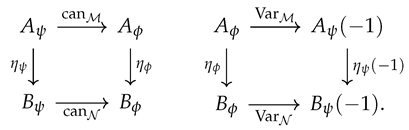
The corresponding monodromy square commutes because $N=\mathrm{Var}\circ \mathrm{can}$ [13]. The smooth resolved family has trivial nearby-cycle monodromy. Proper direct image and the isomorphism ${\eta }_{\psi }$ therefore give $N_{\mathcal{N}}=N_{\mathcal{M}}=0$.

Lemma 2.

The affine $A_1$ surface $S=\{x^2+bc=0\}$ is rationally smooth, and ${\mathbf{1}}_S^H\left[2\right]\simeq {\mathrm{IC}}_S^H$.

Proof. 

The surface is the quotient ${\mathbb{C}}^2/\{\pm 1\}$. Its link is ${\mathbb{RP}}^3$, a rational homology three-sphere. Thus its intersection complex is the shifted constant rational complex. The finite quotient construction gives the corresponding identification of Hodge modules [13]. □

Theorem 2

(Two-step mixed-Hodge specialization and gluing). Let $I={\mathrm{IC}}_S^H$ and $T=j_{p*}{\mathbb{Q}}_p^H(-1)$. The two coefficients have

$$\begin{array}{cccc}\hfill {\mathrm{\Psi }}_f^H\mathcal{M}& \simeq I\oplus T,\hfill & \hfill {\mathrm{\Phi }}_f^H\mathcal{M}& \simeq T,\hfill \\ \hfill {\mathrm{\Psi }}_f^H\mathcal{N}& \simeq I\oplus T,\hfill & \hfill {\mathrm{\Phi }}_f^H\mathcal{N}& =0.\hfill \end{array}$$

The nearby-cycle comparison ${\eta }_{\psi }$ is an isomorphism. Relative to a semismall splitting and this comparison,

$${\mathrm{sp}}_{\mathcal{M}}:I⟶I\oplus T,a⟼(a,0),{\mathrm{can}}_{\mathcal{M}}={pr}_T.$$

Furthermore, ${\mathrm{Var}}_{\mathcal{M}}=0$ and $N_{\mathcal{M}}=0$.

For $\mathcal{N}$, specialization is an isomorphism and ${\mathrm{can}}_{\mathcal{N}}={\mathrm{Var}}_{\mathcal{N}}=N_{\mathcal{N}}=0$.

Proof. 

The nearby and vanishing objects were computed above from proper specialization and the comparison cone. It remains to identify the structural maps.

First, $i^{*}\mathcal{M}[-1]\simeq {\mathbf{1}}_S^H\left[2\right]\simeq I$ by Lemma 2. Proper base change gives $i^{*}\mathcal{N}[-1]\simeq R{m}_{0*}{\mathbf{1}}_{\tilde{S}}^H\left[2\right]\simeq I\oplus T$.

The resolved specialization map is an isomorphism, so ${\mathrm{sp}}_{\mathcal{N}}$ is an isomorphism by proper direct image. Naturality yields

$${\eta }_{\psi }\circ {\mathrm{sp}}_{\mathcal{M}}={\mathrm{sp}}_{\mathcal{N}}\circ i^{*}\eta [-1].$$

The map $i^{*}\eta [-1]$ is the shifted adjunction unit for the central resolution $m_0$. In the pure semismall decomposition, I and T are nonisomorphic simple Hodge modules with different supports. Consequently, ${Hom}_{\mathrm{MHM}\left(S\right)}(I,T)=0$. The T-component of $i^{*}\eta [-1]$ vanishes, while its I-component restricts to the identity on $S\setminus \left\{p\right\}$. By the intermediate-extension property, this component is ${id}_I$.

Thus, under the chosen decomposition, $i^{*}\eta [-1]=({id}_I,0)$. The specialization triangle identifies its cofiber with T, with canonical map ${pr}_T$.

For $\mathcal{N}$, specialization is an isomorphism, hence ${\mathrm{can}}_{\mathcal{N}}=0$ and ${\mathrm{Var}}_{\mathcal{N}}=0$.

Finally, the triviality of nearby-cycle monodromy gives $0=N_{\mathcal{M}}={\mathrm{Var}}_{\mathcal{M}}\circ {\mathrm{can}}_{\mathcal{M}}$. Since ${\mathrm{can}}_{\mathcal{M}}$ is an epimorphism, ${\mathrm{Var}}_{\mathcal{M}}=0$. □

Proposition 15

(Nonsplitting of the coefficient extension). The exact sequence

$$0⟶T_p⟶\mathcal{M}\stackrel{\eta }{\to }\mathcal{N}⟶0$$

is nonsplit. Its Yoneda class ${ϵ}_{\eta }\in {Ext}_{\mathrm{MHM}\left(\mathcal{S}\right)}^1(\mathcal{N},T_p)$ is therefore nonzero.

Proof. 

A splitting would give a retraction $\mathcal{M}\to T_p$. By the closed-immersion adjunction,

$$\begin{array}{cc}\hfill {Hom}_{{\mathsf{D}}_H\left(\mathcal{S}\right)}(\mathcal{M},T_p)& \simeq {Hom}_{D^b\left(\mathrm{MHS}\right)}(k_p^{*}\mathcal{M},{\mathbb{Q}}_p^H(-1))\hfill \\ & \simeq {Hom}_{D^b\left(\mathrm{MHS}\right)}({\mathbb{Q}}_p^H\left[3\right],{\mathbb{Q}}_p^H(-1))\hfill \\ & ={Ext}_{\mathrm{MHS}}^{-3}(\mathbb{Q},\mathbb{Q}(-1))=0.\hfill \end{array}$$

Thus no retraction exists, and ${ϵ}_{\eta }\ne 0$. □

Remark 13.

The pure semismall splitting of $R{m}_{0*}{\mathbf{1}}_{\tilde{S}}^H\left[2\right]$ does not split the relative coefficient extension on $\mathcal{S}$. The two assertions concern different objects and different geometric maps.

5. Three-Step Modifications and Collision Geometry

We construct the ordered $G{L}_3$ modification tower and identify its subregular transverse incidence resolutions with the restrictions of the global invariant-flag forgetful maps. The terminal family has transverse equation $xy=w^3-s^{2}w$, a one-parameter restriction of the type-$A_2$ Brieskorn–Slodowy deformation [29]. The matrix–flag description also fits the type-A affine-Grassmannian framework [30].

5.1. Three Relative Hecke Modification Spaces

Put $B=Spec\mathbb{C}\left[s\right]$, $C_B=Spec\mathbb{C}[z,s]$, and ${\mathcal{E}}_0={\mathcal{O}}_{C_B}^{\oplus 3}$. We consider three length-one modifications supported at $z=0,s,2s$.

Definition 20.

On the framed rank-three quotient chart, multiplication by z is represented by a matrix A with characteristic polynomial $t(t-s)(t-2s)$. The terminal space is

$${\mathcal{X}}_0=\{(A,s)\in M_3\left(\mathbb{C}\right)\times B:\det (tI-A)=t(t-s)(t-2s)\},$$

with its scheme-theoretic characteristic- polynomial equations.

Definition 21.

The complete-chain space ${\mathcal{X}}_2$ parametrizes $(A,s,F_{•})$, with an A-invariant complete flag $0=F_0\subset F_1\subset F_2\subset F_3={\mathbb{C}}^3$ such that A acts on $F_j/F_{j-1}$ by ${\lambda }_j$, where $({\lambda }_1,{\lambda }_2,{\lambda }_3)=(0,s,2s)$.

Definition 22.

The partial-chain space ${\mathcal{X}}_1$ retains $(A,s,F_1)$ with $\dim F_1=1$ and $A{F}_1=0$. The ordered forgetful tower is

$${\mathcal{X}}_2\stackrel{r}{\to }{\mathcal{X}}_1\stackrel{q}{\to }{\mathcal{X}}_0,$$

where r forgets $F_2$ and q forgets $F_1$.

The ordering selects the zero-eigenvalue line first and the s-eigenvalue line in the quotient by $F_1$.

Proposition 16.

The spaces ${\mathcal{X}}_0,{\mathcal{X}}_1,{\mathcal{X}}_2$ are finite-type schemes over B, and $q,r$ are projective. Both are isomorphisms over $s\ne 0$.

Proof. 

The characteristic-polynomial equations define ${\mathcal{X}}_0$ as a closed subscheme of $M_3\times B$. The invariant-line and invariant-flag conditions define ${\mathcal{X}}_1\subset {\mathcal{X}}_0\times Gr(1,3)$ and ${\mathcal{X}}_2\subset {\mathcal{X}}_0\times {Fl}_3$ as closed incidence schemes. Their forgetful maps are projective.

When $s\ne 0$, the eigenvalues are distinct, and the ordered flag is uniquely determined by $F_1=\ker A$ and $F_2=\ker A\oplus \ker (A-sI)$. These constructions are algebraic on the distinct-eigenvalue locus. □

Proposition 17.

The terminal space ${\mathcal{X}}_0$ is a seven-dimensional relative complete intersection, flat over B. The complete-chain space ${\mathcal{X}}_2$ is smooth of dimension seven and flat over B.

Proof. 

The terminal equations are $tr\left(A\right)=3s$, ${\sigma }_2\left(A\right)=2s^2$, and $\det \left(A\right)=0$. For $s\ne 0$, the fiber is a six-dimensional regular semisimple orbit; for $s=0$, it is the six-dimensional nilpotent cone. Thus the three equations have codimension three in the ten-dimensional ambient space. The complete intersection is Cohen–Macaulay, and constant fiber dimension gives flatness by miracle flatness.

For a fixed complete flag, an endomorphism with the prescribed successive eigenvalues has three free strictly upper-triangular entries. Hence ${\mathcal{X}}_2$ is an affine three-space bundle over ${Fl}_3\times B$, proving smoothness, dimension seven, and flatness. □

The central complete-flag map is $T^{*}{Fl}_3\to {\mathcal{N}}_3$, the Springer resolution of the nilpotent cone. It is semismall: the subregular orbit has codimension two and one-dimensional fiber, while the zero orbit has codimension six and three-dimensional flag fiber. The seven-dimensional simultaneous resolution is instead small, as used in Section 6.

5.2. Terminal Local Chart and the Compound $A_2$ Equation

Near a nilpotent matrix of Jordan type $(2,1)$, consider

$$A=\left(\begin{array}{ccc}0& a& d\\ 1& b& e\\ 0& c& f\end{array}\right).$$

Proposition 18.

The characteristic-polynomial equations are $b+f=3s$, $bf-a-ce=2s^2$, and $af-cd=0$.

With $w=f-s$, $x=c$, and $y=-(d+ef)$, the matrix chart is scheme-theoretically isomorphic to ${\mathbb{A}}_e^1\times \mathcal{T}$, where

$$\mathcal{T}=Spec{\displaystyle \frac{\mathbb{C}[x,y,w,s]}{(xy-w(w-s\left)\right(w+s\left)\right)}}.$$

In particular, ${\mathcal{T}}_0=\{xy=w^3\}$.

Proof. 

Direct expansion gives $\det (tI-A)=t^3-(b+f)t^2+(bf-a-ce)t+af-cd$. Equating this with $t(t-s)(t-2s)$ gives the three stated equations.

Substituting $b=3s-f$ and $a=bf-ce-2s^2$ into $af-cd=0$ yields $c(d+ef)=-f(f-s)(f-2s)$. Thus $xy=w(w-s)(w+s)$.

The inverse polynomial formulas are

$$\begin{array}{c}f=w+s,b=2s-w,c=x,\\ d=-y-e(w+s),\\ a=(2s-w)(w+s)-ex-2s^2.\end{array}$$

They satisfy the defining equations and invert the coordinate change. □

The hypersurface is the pullback of $xy=w^3+\alpha w+\beta$ along $(\alpha ,\beta )=(-s^2,0)$ [29].

Proposition 19.

The threefold $\mathcal{T}$ has a unique singular point at the origin; its central fiber is the $A_2$ surface rational double point.

Proof. 

For $F=xy-w^3+s^{2}w$, the critical equations are $x=y=0$, $3w^2=s^2$, and $sw=0$. They force $w=s=0$, while ${F|}_{s=0}=xy-w^3$. □

5.3. Successive Incidence Resolutions

Definition 23.

Let ${\mathcal{T}}_1\subset \mathcal{T}\times {\mathbb{P}}_{[U:V]}^1$ be defined by

$$xV=(w+s)U,w(w-s)V=yU.$$

Write $q_{\mathrm{loc}}:{\mathcal{T}}_1\to \mathcal{T}$ for the projection.

Proposition 20.

The first incidence space has charts

$$\begin{array}{cc}V\ne 0,\tau =U/V:\hfill & x=(w+s)\tau ,\tau y=w(w-s),\hfill \\ U\ne 0,\sigma =V/U:\hfill & w+s=x\sigma ,y=\sigma w(w-s).\hfill \end{array}$$

The $V\ne 0$ chart has one ordinary double point at $\tau =y=w=s=0$; the $U\ne 0$ chart is affine three-space with coordinates $(x,\sigma ,w)$.

The map $q_{\mathrm{loc}}$ is projective, is an isomorphism away from the origin, and has exceptional fiber ${\mathbb{P}}^1$.

Proof. 

On $V\ne 0$, the defining equation is the nondegenerate quadratic form $\tau y-w^2+sw$. On $U\ne 0$, eliminate s by $s=x\sigma -w$, leaving ${\mathbb{A}}_{x,\sigma ,w}^3$.

Projectivity follows from incidence in $\mathcal{T}\times {\mathbb{P}}^1$. Away from the origin the equations uniquely determine $[U:V]$; at the origin they vanish, leaving the reduced fiber ${\mathbb{P}}^1$. □

Definition 24.

Let $\mathcal{V}=\{\tau y=w(w-s\left)\right\}$ be the singular chart of ${\mathcal{T}}_1$. Its second incidence resolution $\tilde{\mathcal{V}}\subset \mathcal{V}\times {\mathbb{P}}_{[P:Q]}^1$ is defined by

$$\tau Q=wP,(w-s)Q=yP.$$

Write $r_{\mathrm{loc}}:\tilde{\mathcal{V}}\to \mathcal{V}$.

Proposition 21.

The second incidence resolution has affine charts

$$\begin{array}{cc}Q\ne 0,u=P/Q:\hfill & \tau =wu,w-s=uy,\hfill \\ P\ne 0,v=Q/P:\hfill & w=\tau v,y=v(w-s).\hfill \end{array}$$

Both charts are smooth affine three-spaces, with free coordinates $(u,y,s)$ and $(\tau ,v,s)$, respectively. The map is a projective small resolution with exceptional fiber ${\mathbb{P}}^1$.

Proof. 

On the first chart, $w=s+uy$ and $\tau =u(s+uy)$; on the second, $w=\tau v$ and $y=v(\tau v-s)$. Projectivity follows from the incidence embedding, and the map is an isomorphism outside the residual ordinary double point. Its exceptional locus is a curve in a smooth threefold, hence no divisor is contracted. □

Remark 14.

Identification with the ordered global tower.The two incidence constructions are the transverse restrictions of the actual forgetful maps q and r. We verify both identifications on the full matrix chart, without imposing $e=0$.

Write $f=w+s$, $b=2s-w$, $c=x$, $d=-y-ef$, and $a=bf-ex-2s^2$. For $v={(v_1,v_2,v_3)}^t\in \ker A$, the equations are

$$v_1=-b{v}_2-e{v}_3,x{v}_2+f{v}_3=0,a{v}_2+d{v}_3=0.$$

Set $[U:V]=[-v_3:v_2]$. The last two relations become $xV=fU$ and $aV-dU=0$. Moreover,

$$aV-dU=(bf-2s^2)V+yU-e(xV-fU).$$

The final term vanishes by the first relation, while $bf-2s^2=-w(w-s)$. Thus the kernel-line equations are exactly $xV=(w+s)U$ and $w(w-s)V=yU$, defining ${\mathcal{T}}_1$. This identifies q with $q_{\mathrm{loc}}$.

For the second stage, work on $V\ne 0$ and put $\tau =U/V$. The kernel line is generated by $\ell ={(-b+e\tau ,1,-\tau )}^t$. Modulo this line, ${\overline{e}}_2=(b-e\tau ){\overline{e}}_1+\tau {\overline{e}}_3$. In the quotient basis $({\overline{e}}_1,{\overline{e}}_3)$, the induced matrix is

$$\overline{A}=\left(\begin{array}{cc}b-e\tau & d+e(b-e\tau )\\ \tau & f+e\tau \end{array}\right).$$

Its trace is $b+f=3s$, as required for quotient eigenvalues $s,2s$.

Write an s-eigenvector of $\overline{A}$ as $P_0{\overline{e}}_1+Q_0{\overline{e}}_3$. The equations $(\overline{A}-sI){(P_0,Q_0)}^t=0$ are

$$\begin{array}{cc}\hfill (s-w-e\tau )P_0+(d+eb-e^2\tau )Q_0& =0,\hfill \\ \hfill \tau P_0+(w+e\tau )Q_0& =0.\hfill \end{array}$$

Make the invertible projective coordinate change $[P:Q]=[-Q_0:P_0+e{Q}_0]$. The second equation becomes $\tau Q=wP$. Substituting $P_0=Q+eP$ and $Q_0=-P$ into the first gives $(s-w-e\tau )Q+(y+ew)P=0$. Using $\tau Q=wP$ cancels the e-terms and yields $(w-s)Q=yP$.

Thus the quotient s-eigenline condition gives precisely $r_{\mathrm{loc}}$, including its projective scheme structure.

It remains to check the complementary $U\ne 0$ chart. Write $\sigma =V/U$, so $f=x\sigma$. A generator of the zero-eigenline is $\ell ={(-b\sigma +e,\sigma ,-1)}^t$. Modulo this line, the classes of $e_1,e_2$ form a quotient basis, with ${\overline{e}}_3=(-b\sigma +e){\overline{e}}_1+\sigma {\overline{e}}_2$. The induced endomorphism is

$$\overline{A}=\left(\begin{array}{cc}0& -2s^2\\ 1& 3s\end{array}\right),\overline{A}-sI=\left(\begin{array}{cc}-s& -2s^2\\ 1& 2s\end{array}\right).$$

The lower-left entry is 1; hence $\overline{A}-sI$ never vanishes on this chart. Its kernel is a unique line, varying regularly with s. Consequently, r is an isomorphism over this entire complementary chart.

The two chart calculations identify the complete transverse tower. Finally, q and r are $G{L}_3$-equivariant, and the chosen slice is transverse to the subregular conjugacy orbit. The Springer–Slodowy transverse-slice description therefore identifies the tower, étale-locally near that orbit, with the product of smooth orbit directions and the transverse incidence tower [29].

Proposition 22.

The composite transverse incidence map $h=q_{\mathrm{loc}}\circ r_{\mathrm{loc}}:{\mathcal{T}}_2\to \mathcal{T}$ is a smooth resolution. Its exceptional fiber over the origin is a reduced nodal curve $E=E_1\cup E_2$, with $E_1,E_2\simeq {\mathbb{P}}^1$ meeting transversely at one point.

Proof. 

The first incidence space has one ordinary double point, resolved by the second incidence map; the complementary first-stage chart is already smooth.

On $\tau y=w(w-s)$, the first exceptional curve is $y=w=s=0$. In the second-resolution chart $w=\tau v$ and $y=v(w-s)$, its strict transform is $v=s=0$. It meets the new exceptional curve at $\tau =v=s=0$, with transverse local branches. □

5.4. Exceptional Fibers and Pure Hodge Contributions

Let $N\in {\mathfrak{gl}}_3$ have Jordan type $(2,1)$, with $N\left(e_2\right)=e_1$ and $N\left(e_1\right)=N\left(e_3\right)=0$.

Proposition 23.

The subregular Springer fiber ${\mathcal{B}}_N$ is a reduced nodal curve $E_1\cup E_2$, with $E_i\simeq {\mathbb{P}}^1$ and $E_1\cap E_2=\left\{\xi \right\}$ transverse.

Proof. 

One has $\ker N=\langle e_1,e_3\rangle$ and $imN=\langle e_1\rangle$. For $F_1\ne \langle e_1\rangle$, the invariant plane is necessarily $F_2=\ker N$, giving $E_1\simeq \mathbb{P}\left(\ker N\right)$.

For $F_1=\langle e_1\rangle$, every plane containing $e_1$ is invariant, giving $E_2\simeq {\mathbb{P}}^1$. The common flag is $\xi =(\langle e_1\rangle ,\ker N)$.

Near $\xi$, write $F_1=\langle e_1+u{e}_3+v{e}_2\rangle$ and $F_2=\langle F_1,e_3+t{e}_2\rangle$. The invariant-line condition gives $v=0$, and invariance of $F_2$ gives $ut=0$. Hence the local fiber scheme is reduced and nodal [29]. □

Proposition 24.

For $E=E_1\cup E_2$,

$$H^0(E,\mathbb{Q})\simeq \mathbb{Q},H^1(E,\mathbb{Q})=0,H^2(E,\mathbb{Q})\simeq \mathbb{Q}{(-1)}^{\oplus 2}.$$

All remaining cohomology groups vanish.

Proof. 

The normalization sequence is $0\to {\mathbb{Q}}_E\to {\mathbb{Q}}_{E_1}\oplus {\mathbb{Q}}_{E_2}\to {\mathbb{Q}}_{\xi }\to 0$. On $H^0$, the last map is $(a,b)\mapsto a-b$ and is surjective. Thus $H^0\left(E\right)=\mathbb{Q}$ and $H^1\left(E\right)=0$.

Degree-two cohomology is the direct sum of $H^2\left(E_1\right)$ and $H^2\left(E_2\right)$. Each is $\mathbb{Q}(-1)$, compatibly with mixed Hodge structures. □

In particular, the Hodge–Deligne polynomial is $E(E;u,v)=1+2uv$ and $\chi \left(E\right)=3$.

For the complete forgetful map $m=q\circ r$ and a subregular point p, proper base change gives

$$i_p^{*}R{m}_{*}{\mathbf{1}}_{{\mathcal{X}}_2}^H\simeq R\Gamma (E,{\mathbf{1}}_E^H).$$

The resulting degree-two contribution $\mathbb{Q}{(-1)}^{\oplus 2}$ is pure, but the central Springer map also has the zero nilpotent orbit with fiber ${Fl}_3$. Its complete global direct-image structure is therefore not determined by the subregular stalk [13,25].

6. Composition Defects and Mixed-Hodge Extensions

Let ${\mathcal{X}}_2\stackrel{r}{\to }{\mathcal{X}}_1\stackrel{q}{\to }{\mathcal{X}}_0$ be the ordered $G{L}_3$ tower of Section 5, and put $m=q\circ r$. Write $f_0:{\mathcal{X}}_0\to B$, $S_0=f_0^{-1}\left(0\right)$, and $i_0:S_0\hookrightarrow {\mathcal{X}}_0$.

We construct the global composition triangle and calculate its transverse realization using Remark 14. The local defect triangle splits, although its three coefficient extensions are nonsplit.

6.1. Three Coefficient Objects in One Category

Definition 25.

The global coefficients, normalized by the dimension seven, are

$${\mathcal{A}}_0={\mathbf{1}}_{{\mathcal{X}}_0}^H\left[7\right],{\mathcal{A}}_1=R{q}_{*}{\mathbf{1}}_{{\mathcal{X}}_1}^H\left[7\right],{\mathcal{A}}_2=R{m}_{*}{\mathbf{1}}_{{\mathcal{X}}_2}^H\left[7\right].$$

Let $u:{\mathcal{A}}_0\to {\mathcal{A}}_1$ be the adjunction unit for q, and let $v:{\mathcal{A}}_1\to {\mathcal{A}}_2$ be the proper direct image of the unit for r, with the same shifts. Their composite $vu$ is the unit for $m=q\circ r$.

Indeed, the composition of units is $id\stackrel{{\eta }_q}{\to }R{q}_{*}{q}^{*}\stackrel{R{q}_{*}{\eta }_r{q}^{*}}{\to }R{q}_{*}R{r}_{*}{r}^{*}{q}^{*}$, which is the unit of $m^{*}⊣R{m}_{*}$.

All three maps are isomorphisms over $s\ne 0$, so their cones are supported on $S_0$. The global simultaneous resolution is small: the subregular and zero orbits have codimensions three and seven in ${\mathcal{X}}_0$, with fiber dimensions one and three, respectively. Thus $2<3$ and $6<7$, and ${\mathcal{A}}_2\simeq {\mathrm{IC}}_{{\mathcal{X}}_0}^H$ by the small-map decomposition theorem [13].

The central Springer resolution is semismall rather than small; its additional strata enter the global comparison objects.

6.2. Three Derived Comparison Defects

Definition 26.

For $a\in \{u,v,vu\}$, define ${\mathfrak{D}}_a=\mathrm{Cone}\left(P_{f_0}^H\left(a\right)\right)\in {\mathsf{D}}_H\left(S_0\right)$. By Proposition 2,

$${\mathfrak{D}}_a\simeq i_0^{!}\mathrm{Cone}\left(a\right).$$

No further shift is included.

6.3. The Composition-Defect Triangle

Proposition 25

(Composition-defect triangle). The adjunction comparisons determine a distinguished triangle

$${\mathfrak{D}}_u⟶{\mathfrak{D}}_{vu}⟶{\mathfrak{D}}_v\stackrel{{\omega }_{q,r}^H}{\to }{\mathfrak{D}}_u\left[1\right].$$

In particular, $\left[{\mathfrak{D}}_{vu}\right]=\left[{\mathfrak{D}}_u\right]+\left[{\mathfrak{D}}_v\right]$ in $K_0\left({\mathsf{D}}_H\left(S_0\right)\right)$.

Proof. 

The octahedral construction for ${\mathcal{A}}_0\stackrel{u}{\to }{\mathcal{A}}_1\stackrel{v}{\to }{\mathcal{A}}_2$ gives $\mathrm{Cone}\left(u\right)\to \mathrm{Cone}\left(vu\right)\to \mathrm{Cone}\left(v\right)\to \mathrm{Cone}\left(u\right)\left[1\right]$. Applying the exact functor $i_0^{!}$ produces the asserted triangle. Its connecting morphism is ${\omega }_{q,r}^H=i_0^{!}\delta$, where $\delta$ is the connecting morphism of the coefficient cones.

The Grothendieck-group identity follows from the triangle. □

The class ${\omega }_{q,r}^H$ is not determined by the Grothendieck-group identity. It is a morphism in the derived mixed-Hodge-module category, and its calculation requires the supported comparison objects.

6.4. Nonformal Calculation of the Defect Pieces

Let $\mathcal{T}=\{xy=w(w-s\left)\right(w+s\left)\right\}$, with ordered transverse tower ${\mathcal{T}}_2\stackrel{r_{\mathrm{loc}}}{\to }{\mathcal{T}}_1\stackrel{q_{\mathrm{loc}}}{\to }\mathcal{T}$, and put $h=q_{\mathrm{loc}}\circ r_{\mathrm{loc}}$.

By Remark 14, these maps are the transverse restrictions of the ordered global forgetful maps.

Define the local coefficients

$$A_0={\mathbf{1}}_{\mathcal{T}}^H\left[3\right],A_1=R{q}_{\mathrm{loc}*}{\mathbf{1}}_{{\mathcal{T}}_1}^H\left[3\right],A_2=R{h}_{*}{\mathbf{1}}_{{\mathcal{T}}_2}^H\left[3\right].$$

Let $u_{\mathrm{loc}}:A_0\to A_1$ and $v_{\mathrm{loc}}:A_1\to A_2$ be their adjunction comparisons.

Write p for the origin of $\mathcal{T}$, $k_p:\left\{p\right\}\hookrightarrow \mathcal{T}$, and $T_p=k_{p*}{\mathbb{Q}}_p^H(-1)$. The object $T_p$ is a pure point-supported Hodge module of weight two.

Proposition 26.

For a proper morphism $g:Y\to X$ with shifted adjunction unit ${\eta }_g:{\mathbf{1}}_X^H\left[d\right]\to R{g}_{*}{\mathbf{1}}_Y^H\left[d\right]$, one has

$$i_x^{*}\mathrm{Cone}\left({\eta }_g\right)\simeq \mathrm{Cone}\left({\mathbb{Q}}_x^H\left[d\right]⟶R\Gamma (g^{-1}\left(x\right),{\mathbf{1}}^H)\left[d\right]\right).$$

Proof. 

Apply $i_x^{*}$ to the adjunction triangle and use proper base change. The induced map is the shifted structural unit of the fiber [13]. □

For the complete map m, the subregular Springer fiber has $H^2(E,\mathbb{Q})\simeq \mathbb{Q}{(-1)}^{\oplus 2}$. The corresponding stalk cone uses shift $\left[5\right]$ on the global seven-dimensional family and $\left[1\right]$ on the transverse threefold: in each case the unshifted exceptional contribution is $\mathbb{Q}{(-1)}^{\oplus 2}[-2]$. At the zero orbit, the global fiber is ${Fl}_3$, so the global cone has additional supported data.

Proposition 27.

For the transverse incidence tower,

$$\mathrm{Cone}\left(u_{\mathrm{loc}}\right)\simeq T_p\left[1\right],\mathrm{Cone}\left(v_{\mathrm{loc}}\right)\simeq T_p\left[1\right],\mathrm{Cone}\left(v_{\mathrm{loc}}{u}_{\mathrm{loc}}\right)\simeq T_p^{\oplus 2}\left[1\right].$$

Their variation-comparison defects on ${\mathcal{T}}_0$ are the corresponding point-supported objects, with the same shifts and Tate twists.

Proof. 

The map $q_{\mathrm{loc}}$ is an isomorphism away from p, with fiber ${\mathbb{P}}^1$ over p. By Proposition 26, its stalk comparison cone is

$$\mathrm{Cone}\left({\mathbb{Q}}_p^H\left[3\right]\to R\Gamma ({\mathbb{P}}^1,{\mathbf{1}}^H)\left[3\right]\right).$$

Since $R\Gamma ({\mathbb{P}}^1,{\mathbf{1}}^H)\simeq {\mathbb{Q}}^H\oplus {\mathbb{Q}}^H(-1)[-2]$ and the unit is an isomorphism on $H^0$, the cone is ${\mathbb{Q}}_p^H(-1)\left[1\right]$. It is supported at p, giving $\mathrm{Cone}\left(u_{\mathrm{loc}}\right)\simeq T_p\left[1\right]$.

For the second map $r_{\mathrm{loc}}$, the only exceptional fiber is ${\mathbb{P}}^1$ over the residual ordinary double point $p_1$. The same stalk calculation gives $\mathrm{Cone}\left({\eta }_{r_{\mathrm{loc}}}\left[3\right]\right)\simeq k_{p_1*}{\mathbb{Q}}_{p_1}^H(-1)\left[1\right]$. Applying $R{q}_{\mathrm{loc}*}$ and using $q_{\mathrm{loc}}\left(p_1\right)=p$ gives $\mathrm{Cone}\left(v_{\mathrm{loc}}\right)\simeq T_p\left[1\right]$.

Finally, $h^{-1}\left(p\right)=E_1\cup E_2$ with $H^0(E,\mathbb{Q})=\mathbb{Q}$, $H^1(E,\mathbb{Q})=0$, and $H^2(E,\mathbb{Q})=\mathbb{Q}{(-1)}^{\oplus 2}$ by Proposition 24. The composite unit is the identity on degree-zero cohomology; hence $\mathrm{Cone}\left(v_{\mathrm{loc}}{u}_{\mathrm{loc}}\right)\simeq T_p^{\oplus 2}\left[1\right]$.

All cones are supported on $\left\{p\right\}$, so extraordinary restriction to ${\mathcal{T}}_0$ preserves these point-supported descriptions. □

6.5. The Connecting Morphism and Extension Question

Corollary 4.

The transverse connecting morphism vanishes, ${\omega }_{\mathrm{loc}}^H=0$. Consequently its composition-defect triangle splits:

$${\mathfrak{D}}_{vu}^{\mathrm{loc}}\simeq {\mathfrak{D}}_u^{\mathrm{loc}}\oplus {\mathfrak{D}}_v^{\mathrm{loc}}\simeq j_{p*}{\mathbb{Q}}_p^H{(-1)}^{\oplus 2}\left[1\right],$$

where $j_p:\left\{p\right\}\hookrightarrow {\mathcal{T}}_0$.

Proof. 

The outer defects are both $j_{p*}{\mathbb{Q}}_p^H(-1)\left[1\right]$. The connecting morphism lies in

$${Hom}_{D^b\left(\mathrm{MHS}\right)}\left(\mathbb{Q}(-1)\left[1\right],\mathbb{Q}(-1)\left[2\right]\right)={Ext}_{\mathrm{MHS}}^1(\mathbb{Q}(-1),\mathbb{Q}(-1)).$$

This group vanishes by semisimplicity of polarizable pure Hodge structures of fixed weight [5]. Thus ${\omega }_{\mathrm{loc}}^H=0$, and the distinguished triangle splits. □

This argument is point-supported and does not determine the global class ${\omega }_{q,r}^H$, whose objects have additional nilpotent-orbit support. In particular, the local computation does not assert global vanishing.

6.6. Coefficient Extensions Versus Defect-Triangle Splitting

For a morphism $a:L\to M$ in $\mathrm{MHM}\left(Y\right)$ with $\mathrm{Cone}\left(a\right)\simeq T\left[1\right]$, standard cohomology gives the short exact sequence $0\to T\to L\stackrel{a}{\to }M\to 0$. We apply this observation to the three transverse comparisons.

Proposition 28.

The coefficient objects $A_0,A_1,A_2$ belong to $\mathrm{MHM}\left(\mathcal{T}\right)$ and fit into exact sequences

$$\begin{array}{c}0⟶T_p⟶A_0\stackrel{u_{\mathrm{loc}}}{\to }{A}_1⟶0,\\ 0⟶T_p⟶A_1\stackrel{v_{\mathrm{loc}}}{\to }{A}_2⟶0,\\ 0⟶T_p^{\oplus 2}⟶A_0\stackrel{v_{\mathrm{loc}}{u}_{\mathrm{loc}}}{\to }{A}_2⟶0.\end{array}$$

All three sequences are nonsplit.

Proof. 

The threefold $\mathcal{T}$ is a pure-dimensional local complete intersection. Hence $A_0={\mathbf{1}}_{\mathcal{T}}^H\left[3\right]$ is perverse.

The cone identifications of Proposition 27 and the standard cohomology sequence give $A_1,A_2\in \mathrm{MHM}\left(\mathcal{T}\right)$ and the three displayed exact sequences.

To prove nonsplitting, use the closed-immersion adjunction

$${Hom}_{{\mathsf{D}}_H\left(\mathcal{T}\right)}(A_j,T_p)\simeq {Hom}_{D^b\left(\mathrm{MHS}\right)}(k_p^{*}{A}_j,{\mathbb{Q}}_p^H(-1)).$$

For the first sequence, $k_p^{*}{A}_0\simeq {\mathbb{Q}}_p^H\left[3\right]$, so

$${Hom}_{{\mathsf{D}}_H\left(\mathcal{T}\right)}(A_0,T_p)\simeq {Ext}_{\mathrm{MHS}}^{-3}(\mathbb{Q},\mathbb{Q}(-1))=0.$$

There can be no retraction $A_0\to T_p$.

For the second sequence, proper base change gives $k_p^{*}{A}_1\simeq R\Gamma ({\mathbb{P}}^1,{\mathbf{1}}^H)\left[3\right]\simeq {\mathbb{Q}}_p^H\left[3\right]\oplus {\mathbb{Q}}_p^H(-1)\left[1\right]$. Consequently,

$$\begin{array}{cc}\hfill {Hom}_{{\mathsf{D}}_H\left(\mathcal{T}\right)}(A_1,T_p)\simeq & {Ext}_{\mathrm{MHS}}^{-3}(\mathbb{Q},\mathbb{Q}(-1))\hfill \\ & \oplus {Ext}_{\mathrm{MHS}}^{-1}(\mathbb{Q}(-1),\mathbb{Q}(-1))=0.\hfill \end{array}$$

Thus the second inclusion has no retraction either.

Finally, ${Hom}_{{\mathsf{D}}_H\left(\mathcal{T}\right)}(A_0,T_p^{\oplus 2})=0$ by the first calculation. The composite sequence is nonsplit.

Writing ${ϵ}_a^H$ for each Yoneda class, all three are nonzero. □

Theorem 3

(Local splitting versus coefficient nonsplitting). For the transverse compound-$A_2$ incidence tower identified with the ordered $G{L}_3$ modification tower in Remark 14, the dimension-three-normalized coefficient comparisons satisfy:

1.

$\mathrm{Cone}\left(u_{\mathrm{loc}}\right)\simeq T_p\left[1\right]$, $\mathrm{Cone}\left(v_{\mathrm{loc}}\right)\simeq T_p\left[1\right]$, and $\mathrm{Cone}\left(v_{\mathrm{loc}}{u}_{\mathrm{loc}}\right)\simeq T_p^{\oplus 2}\left[1\right]$.

2.

The composition-defect triangle splits, with ${\omega }_{\mathrm{loc}}^H=0$.

3.

The three coefficient comparisons give nonsplit short exact sequences in $\mathrm{MHM}\left(\mathcal{T}\right)$, with kernels $T_p$, $T_p$, and $T_p^{\oplus 2}$.

Proof. 

The geometric identification is Remark 14. The cone calculations are Proposition 27; the connecting morphism is calculated in Corollary 4; and the heart-level nonsplitting is Proposition 28. □

The theorem distinguishes the vanishing derived composition class ${\omega }_{\mathrm{loc}}^H$ from the nonzero coefficient Yoneda classes ${ϵ}_{u_{\mathrm{loc}}}^H$, ${ϵ}_{v_{\mathrm{loc}}}^H$, and ${ϵ}_{v_{\mathrm{loc}}{u}_{\mathrm{loc}}}^H$. The global class ${\omega }_{q,r}^H$ remains a separate problem involving the nilpotent-orbit stratification.

7. Bivariant Interpretation and Singular Hodge Atoms

The preceding calculations identify two distinct forms of mixed-Hodge extension information. In the two-step collision, coefficient objects with isomorphic nearby cycles have different canonical and vanishing-cycle maps. In the transverse three-step collision, the derived composition-defect triangle splits while the coefficient extensions remain nonsplit.

We interpret these results in relation to the author’s singular Hodge-atom constructions, which retain vanishing-cycle sectors, perverse extensions, monodromy, and the morphisms attaching singular contributions to ambient Hodge modules [17,18,19,20].

7.1. What the Comparison Construction Retains

Let $f:X\to B$ be a morphism to a smooth curve, with distinguished-fiber inclusion $i:X_0\hookrightarrow X$.

Definition 27.

For $a:{\mathcal{L}}_0\to {\mathcal{L}}_1$ in ${\mathsf{D}}_H\left(X\right)$, the derived coefficient-comparison datum is

$$\mathfrak{C}\left(a\right)=({\mathcal{L}}_0,{\mathcal{L}}_1,a,\mathrm{Cone}\left(a\right)).$$

Its specialization includes the induced maps ${\mathrm{\Psi }}_f^H\left(a\right)$ and ${\mathrm{\Phi }}_f^H\left(a\right)$, together with their canonical, variation, and monodromy compatibility.

The associated defect is ${\mathfrak{D}}_f\left(a\right)=\mathrm{Cone}\left(P_f^H\left(a\right)\right)\simeq i^{!}\mathrm{Cone}\left(a\right)$.

The final identity is the functorial variation-cone isomorphism of Proposition 2. It shows that the defect is supported on $X_0\cap Supp\mathrm{Cone}\left(a\right)$. For composable comparisons, the octahedral triangle of Proposition 25 retains their connecting morphism, not merely the corresponding Grothendieck-group identity.

Remark 15.

Theorem 2 shows that the nearby-cycle object alone does not determine the specialization package: $\mathcal{M}$ and $\mathcal{N}$ have isomorphic nearby cycles, but different canonical maps and vanishing-cycle objects.

Theorem 3 shows that a split triangle of supported defects need not split the underlying coefficient extensions. Thus neither the nearby-cycle isomorphism class nor the Grothendieck class of a comparison cone determines its coefficient-level extension behavior.

Remark 16.

Herebivariantdenotes dependence on specified geometric morphisms, their adjunction coefficient maps, and composition. This is related to, but does not define, a complete Fulton–MacPherson bivariant theory [26,27].

7.2. Relationship with the Variation-Cone Hodge-Atom Program

The singular Hodge-atom program studies nearby and vanishing cycles, perverse extensions, rigid–flexible decomposition, and global gluing under degeneration [17,18,19,20].

The present Hecke calculations employ Saito’s same specialization operations, but attach the coefficient maps to ordered geometric modifications [13].

For $\mathcal{L}\in {\mathsf{D}}_H\left(X\right)$, write ${\mathfrak{A}}_f^H\left(\mathcal{L}\right)=({\mathrm{\Psi }}_f^H\mathcal{L},{\mathrm{\Phi }}_f^H\mathcal{L},{\mathrm{can}}_{\mathcal{L}},{\mathrm{Var}}_{\mathcal{L}},N_{\mathcal{L}})$. Every coefficient morphism induces a morphism of these packages by naturality of the canonical and variation maps. In particular, ${\mathrm{\Phi }}_f^H\left(a\right){\mathrm{can}}_{{\mathcal{L}}_0}={\mathrm{can}}_{{\mathcal{L}}_1}{\mathrm{\Psi }}_f^H\left(a\right)$, and ${\mathrm{\Psi }}_f^H\left(a\right)(-1){\mathrm{Var}}_{{\mathcal{L}}_0}={\mathrm{Var}}_{{\mathcal{L}}_1}{\mathrm{\Phi }}_f^H\left(a\right)$.

Definition 28.

Let $\mathcal{R},\mathcal{F},\mathcal{P}\in \mathrm{MHM}\left(Y\right)$ be the rigid, flexible, and carrier objects of a specified singular Hodge-atom construction, with short exact sequence

$$0⟶\mathcal{R}⟶\mathcal{P}⟶\mathcal{F}⟶0.$$

Arigid–flexible comparisonis an isomorphism between this exact sequence and a geometrically defined Hecke coefficient extension in a common mixed-Hodge-module category, compatible with support, Tate twists, and the relevant specialization maps. It therefore identifies the Yoneda classes in ${Ext}_{\mathrm{MHM}\left(Y\right)}^1(\mathcal{F},\mathcal{R})$.

Proposition 29.

A rigid–flexible comparison identifies the Hecke coefficient extension with the specified atomic carrier extension, including its Yoneda class. An identification of nearby-cycle, vanishing-cycle, or graded Hodge objects alone is insufficient.

Proof. 

An isomorphism of short exact sequences identifies their Yoneda classes. Compatibility with specialization preserves canonical and variation maps. Isomorphisms of the individual cycle objects do not determine these morphisms or the extension sequence. □

The exceptional Tate contributions in the two-step and three-step models are $\mathbb{Q}(-1)$ and $\mathbb{Q}{(-1)}^{\oplus 2}$. They become specific atomic data only after a comparison with the corresponding rigid–flexible carrier and its extension morphism has been established.

7.3. Scope of the Local Result

The comparison construction is natural under compatible morphisms of coefficient diagrams. Invariance under changes of Hecke presentation, and extension to general convolution categories, requires the corresponding geometric identifications and convolution coherence.

The affine-Grassmannian background is provided by geometric Satake [2,3]. The present results establish local mixed-Hodge-module comparisons, not a general Hecke action on singular Hodge-atom carriers or a geometric-Langlands correspondence.

The mathematical conclusion is that **coefficient extensions and derived composition defects constitute distinct data**: the local examples show they can have different splitting behavior. A correspondence-level realization of singular Hodge atoms must therefore preserve the relevant coefficient morphisms, not only the cohomology of their exceptional fibers.

8. Outlook: Coherent Realizations and Line Operators

The local coefficient comparisons suggest two immediate mathematical problems: extending the incidence calculation to higher type-A towers and determining the global composition obstruction on the $G{L}_3$ nilpotent cone. They also provide explicit tests for coherent realizations and Hecke–Hitchin transformations.

8.1. From Bounded Fusion to Genuine Hecke Actions

Let C be a smooth projective curve and G a connected reductive group. The Hecke correspondence over ${Bun}_G\left(C\right)$ is organized by affine-Grassmannian convolution and geometric Satake [2,3].

For a finite-type Hecke correspondence $p_1,p_2:\mathcal{H}\to \mathcal{B}$ with suitable mixed-Hodge-module operations, a kernel $\mathcal{K}\in {\mathsf{D}}_H\left(\mathcal{H}\right)$ defines the prospective transform ${\mathsf{H}}_{\mathcal{K}}\left(\mathcal{L}\right)=p_{2!}(p_1^{*}\mathcal{L}\otimes \mathcal{K})$. Compatibility with collision specialization would require natural comparisons intertwining this transform with nearby and vanishing cycles, their canonical and variation maps, monodromy, and convolution associativity.

The first concrete extension is the ordered type-$A_{n-1}$ collision along the eigenvalue line $(0,s,\dots ,(n-1\left)s\right)$. Its natural subregular transverse model is expected to take the form

$${\mathcal{T}}_n:xy={\displaystyle \prod _{j=0}^{n-1}}(w-js),$$

with central surface $xy=w^n$. The subregular Springer fiber is an $A_{n-1}$ chain of $n-1$ projective lines, giving $H^2(E,\mathbb{Q})\simeq \mathbb{Q}{(-1)}^{\oplus (n-1)}$ [29].

To generalize Theorem 3, one must identify each successive ordered incidence map and calculate its adjunction cone. Only after those calculations can one test whether the corresponding composition defects split and whether the coefficient extensions remain nonsplit.

Remark 17.

A separate problem is the global composition class ${\omega }_{q,r}^H\in {Hom}_{{\mathsf{D}}_H\left(S_0\right)}({\mathfrak{D}}_v,{\mathfrak{D}}_u\left[1\right])$ for the $G{L}_3$ simultaneous-resolution tower.

The subregular transverse defects are supported at one point. Globally, the nilpotent cone also contains the zero orbit, whose Springer fiber is ${Fl}_3$. The global class consequently depends on orbit-closure extension and gluing data not detected by the pure point-supported calculation.

Its vanishing or nonvanishing is not established in this paper.

8.2. The Constructible–Coherent Interface

The filtered $\mathcal{D}$-modules underlying mixed Hodge modules provide one route toward coherent data [13,38]. Affine-Hecke coherent realizations and singular-support methods provide other, categorically distinct approaches [37,39].

Definition 29.

For a smooth variety Y and a filtered left ${\mathcal{D}}_Y$-module $(M,F_{•}M)$, define

$${\mathcal{R}}_F\left(M\right)=\underset{p\in \mathbb{Z}}{⨁}{F}_{p}M{\hslash }^p,{\mathcal{R}}_F\left({\mathcal{D}}_Y\right)=\underset{p\ge 0}{⨁}{F}_p{\mathcal{D}}_Y{\hslash }^p.$$

Specialization at $\hslash =1$ recovers M, while specialization at $\hslash =0$ gives ${gr}^{F}M$. For a good filtration, ${gr}^{F}M$ is coherent over ${gr}^F{\mathcal{D}}_Y\simeq {Sym}_{{\mathcal{O}}_Y}\left({\mathcal{T}}_Y\right)$.

Remark 18.

For a strict short exact sequence $0\to M^{\prime }\to M\to M^{\prime \prime }\to 0$ of filtered ${\mathcal{D}}_Y$-modules, both the Rees sequence

$$0⟶{\mathcal{R}}_F\left(M^{\prime }\right)⟶{\mathcal{R}}_F\left(M\right)⟶{\mathcal{R}}_F\left(M^{\prime \prime }\right)⟶0$$

and the associated graded sequence are exact. Indeed, strictness gives exactness of $0\to F_p{M}^{\prime }\to F_{p}M\to F_p{M}^{\prime \prime }\to 0$ at every filtration level. Taking graded direct sums yields Rees exactness, while successive filtration quotients yield the associated graded exact sequence.

Remark 19.

The filtered $\mathcal{D}$-module component does not independently retain the rational perverse sheaf or its comparison with the de Rham realization. Consequently, an associated graded extension need not determine the original Yoneda class in $\mathrm{MHM}\left(Y\right)$.

A coherent realization of the nonsplitting results must therefore preserve, or faithfully detect, the underlying coefficient extension class.

A prospective exact realization ${\mathsf{R}}_{\mathrm{coh}}:{\mathcal{C}}_H\to {\mathcal{C}}_{\mathrm{coh}}$ would need to transport a specified coefficient comparison triangle to its coherent counterpart. Compatibility with specialization additionally requires comparison morphisms for nearby and vanishing cycles and their structural maps. These properties are not consequences of the Rees construction alone.

8.3. Hitchin Degenerations and Kapustin–Witten Motivation

Let $h_G:{\mathcal{M}}_{\mathrm{Higgs}}\left(G\right)\to {\mathcal{A}}_G$ denote a Hitchin fibration. Its integrable-system geometry, duality, and global Springer theory provide natural settings for singular modification correspondences [40,41,42].

In the Kapustin–Witten framework, Wilson and ’t Hooft line operators are related to tensor-type and Hecke-modification operations [43]. A Hodge-theoretic comparison of such operations would need to transport their coefficient morphisms and specialization packages through a specified Hecke–Hitchin degeneration.

Remark 20.

Let $a:{\mathcal{L}}_0\to {\mathcal{L}}_1$ be a coefficient comparison over $f:Y\to B$, with distinguished-fiber inclusion $i:Y_0\hookrightarrow Y$. Suppose exact functors $\mathsf{T}:{\mathcal{C}}_H\to {\mathcal{C}}^{\prime }$ and ${\mathsf{T}}_0:{\mathcal{C}}_{H,0}\to {\mathcal{C}}_0^{\prime }$ are defined on the relevant total- and special-fiber categories, with a natural isomorphism ${\mathsf{T}}_0\circ i^{!}\simeq i^{\prime !}\circ \mathsf{T}$.

If the target categories admit compatible variation-cone identifications, then

$${\mathsf{T}}_0\left({\mathfrak{D}}_f\left(a\right)\right)\simeq {\mathfrak{D}}_{f^{\prime }}\left(\mathsf{T}\left(a\right)\right).$$

Indeed, by Proposition 2, exactness of $\mathsf{T}$, and compatibility with extraordinary restriction,

$$\begin{array}{cc}\hfill {\mathsf{T}}_0\left({\mathfrak{D}}_f\left(a\right)\right)& \simeq {\mathsf{T}}_0\left(i^{!}\mathrm{Cone}\left(a\right)\right)\hfill \\ & \simeq i^{\prime !}\mathsf{T}\left(\mathrm{Cone}\left(a\right)\right)\hfill \\ & \simeq i^{\prime !}\mathrm{Cone}\left(\mathsf{T}\left(a\right)\right)\hfill \\ & \simeq {\mathfrak{D}}_{f^{\prime }}\left(\mathsf{T}\left(a\right)\right).\hfill \end{array}$$

Thus defect transport follows formally from the stated compatibility hypotheses.

Preservation of nonsplit coefficient extensions requires more: the categorical realization must also detect the nonzero Yoneda classes of the original extensions. Exact transport of derived defects alone does not establish this property.

The higher type-A collision construction and global Springer composition obstruction are immediate mathematical continuations of the present results. Coherent Hecke realizations and Hitchin line-operator comparisons provide longer-term settings in which to test the preservation of morphism-sensitive mixed-Hodge extension data.

Appendix A.1. Two-Step Characteristic-Polynomial Chart

The framed length-two quotient has multiplication matrix $A=\left(\begin{array}{cc}a& b\\ c& s-a\end{array}\right)$. Its characteristic-polynomial condition $a(s-a)=bc$ becomes $xy=bc$, where $x=a$, $y=s-a$, and $s=x+y$.

For the kernel-line resolution, the equations $xu+bv=cu+yv=0$ give the two affine charts

On the overlap, $w=t^{-1}$, $x=-bt$, and $c=-yt$. The normal directions of the exceptional curve therefore transform with degree $-1$, giving $N_{E/\tilde{\mathcal{S}}}\simeq {\mathcal{O}}_{{\mathbb{P}}^1}{(-1)}^{\oplus 2}$.

On the central fiber, $s=0$ gives $y=bt$ and $c=-b{t}^2$. Thus $N_{E/{\tilde{\mathcal{S}}}_0}\simeq {\mathcal{O}}_{{\mathbb{P}}^1}(-2)$.

These calculations provide the transitions used in Propositions 10 and 11.

Remark A1.

The affine central resolution is $Tot\left({\mathcal{O}}_{{\mathbb{P}}^1}(-2)\right)$. Its natural projective completion is ${\mathbb{F}}_2$, the convolution surface of Proposition 6.

The two surfaces have the same exceptional neighborhood but are not identical global geometric spaces.

Appendix A.2. Three-Step Characteristic-Polynomial Chart

Near a subregular nilpotent matrix, use

$$A=\left(\begin{array}{ccc}0& a& d\\ 1& b& e\\ 0& c& f\end{array}\right).$$

The characteristic-polynomial condition $\det (tI-A)=t(t-s)(t-2s)$ gives $b+f=3s$, $bf-a-ce=2s^2$, and $af-cd=0$.

The coordinates $w=f-s$, $x=c$, and $y=-(d+ef)$ have polynomial inverse

$$\begin{array}{c}f=w+s,b=2s-w,c=x,\\ d=-y-e(w+s),\\ a=(2s-w)(w+s)-ex-2s^2.\end{array}$$

They identify the displayed matrix chart with ${\mathbb{A}}_e^1\times \mathcal{T}$, where $\mathcal{T}=\{xy=w^3-s^{2}w\}$.

The central transverse surface is $xy=w^3$. This is the restriction of the Brieskorn–Slodowy deformation $xy=w^3+\alpha w+\beta$ along $(\alpha ,\beta )=(-s^2,0)$ [29].

The scheme-theoretic identification is established in Proposition 18.

Appendix A.3. Successive Incidence Charts

For the ordered eigenvalues $(0,s,2s)$, the first incidence equations are $xV=(w+s)U$ and $w(w-s)V=yU$. On $V\ne 0$, with $\tau =U/V$, they become $x=(w+s)\tau$ and $\tau y=w(w-s)$; on $U\ne 0$, with $\sigma =V/U$, they become $w+s=x\sigma$ and $y=\sigma w(w-s)$.

The residual ordinary double point $\mathcal{V}=\{\tau y=w(w-s\left)\right\}$ is resolved by $\tau Q=wP$ and $(w-s)Q=yP$. The corresponding smooth affine charts are

On the overlap, $uv=1$ and $w=s+uy=\tau v$.

These equations give the smooth resolution and nodal exceptional fiber of Propositions 21 and 22.

Remark A2.

The local resolutions are not merely abstract resolutions of the same compound-$A_2$ singularity.

Remark 14 identifies the first incidence map with the zero-eigenline condition on the full ${\mathbb{A}}_e^1\times \mathcal{T}$ matrix chart. The second incidence map is obtained from the s-eigenline of the quotient endomorphism on $Q/F_1$.

The proof includes the invertible projective-coordinate change on the $V\ne 0$ chart and the nonvanishing of $\overline{A}-sI$ on the complementary $U\ne 0$ chart.

Since the global forgetful maps are $G{L}_3$-equivariant and the chosen slice is transverse to the subregular orbit, the Springer–Slodowy local product description identifies the ordered tower étale-locally with its transverse incidence model [29].

References

- Gaitsgory, D. Construction of Central Elements in the Affine Hecke Algebra via Nearby Cycles. Invent. Math. 2001, 144, 253–280. [Google Scholar] [CrossRef]
- Mirković, I.; Vilonen, K. Geometric Langlands duality and representations of algebraic groups over commutative rings. Ann. Math. 2007, 166, 95–143. [Google Scholar] [CrossRef]
- Fedorov, R. Satake equivalence for Hodge modules on affine Grassmannians. arXiv 2021, arXiv:math. [Google Scholar] [CrossRef]
- Bondal, A.; Kapranov, M.; Schechtman, V. Perverse Schobers and Birational Geometry. arXiv 2018, arXiv:math. [Google Scholar] [CrossRef]
- Deligne, P. Théorie de Hodge. II. Publ. Mathématiques De l’Institut Des. Hautes Études Sci. 1971, 40, 5–57. [Google Scholar] [CrossRef]
- Deligne, P. Théorie de Hodge. III. Publ. Mathématiques De l’Institut Des. Hautes Études Sci. 1974, 44, 5–77. [Google Scholar] [CrossRef]
- Schmid, W. Variation of Hodge Structure: The Singularities of the Period Mapping. Invent. Math. 1973, 22, 211–319. [Google Scholar] [CrossRef]
- Steenbrink, J.H.M. Limits of Hodge structures. Invent. Math. 1976, 31, 229–257. [Google Scholar] [CrossRef]
- Peters, C.A.M.; Steenbrink, J.H.M. Mixed Hodge Structures . In Ergebnisse der Mathematik und ihrer Grenzgebiete; Springer: Berlin, 2008; Vol. 52. [Google Scholar] [CrossRef]
- Beilinson, A.A.; Bernstein, J.; Deligne, P. Faisceaux pervers; Société Mathématique de France: Astérisque , 1982; Vol. 100. [Google Scholar]
- Beilinson, A.A. How to glue perverse sheaves. K-Theory 1987, 1, 91–107. [Google Scholar] [CrossRef]
- Saito, M. Modules de Hodge polarisables. Publ. Res. Inst. Math. Sci. 1988, 24, 849–995. [Google Scholar] [CrossRef]
- Saito, M. Mixed Hodge Modules. Publ. Res. Inst. Math. Sci. 1990, 26, 221–333. [Google Scholar] [CrossRef]
- Katzarkov, L.; Kontsevich, M.; Pantev, T.; Yu, T.Y. Birational Invariants from Hodge Structures and Quantum Multiplication, 2025. Found. Hodge-At. Constr. arXiv subsequently revised. arXiv:math. [CrossRef]
- Cavenaghi, L.F.; Katzarkov, L.; Kontsevich, M. Atoms meet symbols, 2025. Equivariant Birational Geom. Modul. Symb. Chen–Ruan At. arXiv:math. [CrossRef]
- Alexeev, B.; Cavenaghi, L.F.; Galindo, G.; Georgiev, B.; Katzarkov, L.; Martins, P.A.M. On the Atomic Decomposition of Complete Intersection in Flag Varieties, 2026. arXiv arXiv:math. [CrossRef]
- Rahman, A. Hodge Atoms at Conifold Degenerations: F-Bundles, Limiting Mixed Hodge Modules, and the Rigid–Flexible Decomposition, 2026. arXiv arXiv:math. [CrossRef]
- Rahman, A. Perverse Extensions and Limiting Mixed Hodge Structures for Conifold Degenerations, 2026. arXiv arXiv:math. [CrossRef]
- Rahman, A. Mixed Hodge Modules and Canonical Perverse Extensions for Multi-Node Conifold Degenerations. arXiv 2026, arXiv:math. [Google Scholar] [CrossRef]
- Rahman, A. Cycle Relations and Global Gluing in Multi-Node Conifold Degenerations, 2026. arXiv arXiv:math. [CrossRef]
- Rahman, A. Equivariant Hodge Atoms at Conifold Degenerations. Preprints.org, 2026. Version 1. 2026. [Google Scholar]
- Rahman, A. Equivariant Gluing at Conifold Degenerations: Local Extension Channels and Global Relation Sectors. Preprints.org, Version 1; 2026. [Google Scholar]
- Ginzburg, V. Perverse sheaves on a loop group and Langlands’ duality. arXiv 1995. [Google Scholar]
- Beilinson, A.; Drinfeld, V. Chiral Algebras . In American Mathematical Society Colloquium Publications; American Mathematical Society, 2004; Vol. 51. [Google Scholar]
- de Cataldo, M.A.A.; Migliorini, L. The Hard Lefschetz Theorem and the Topology of Semismall Maps. Ann. Sci. De l’École Norm. Supérieure 2002, 35, 759–772. [Google Scholar] [CrossRef]
- Fulton, W.; MacPherson, R. Categorical framework for the study of singular spaces. Mem. Am. Math. Soc. 1981, 31. [Google Scholar] [CrossRef]
- Fulton, W. Intersection Theory . In Ergebnisse der Mathematik und ihrer Grenzgebiete, 2 ed.; Springer, 1998; Vol. 2. [Google Scholar]
- Atiyah, M.F. On Analytic Surfaces with Double Points. Proc. R. Soc. London. Ser. A 1958, 247, 237–244. [Google Scholar] [CrossRef]
- Slodowy, P. Simple Singularities and Simple Algebraic Groups . In Lecture Notes in Mathematics; Springer: Berlin, 1980; Vol. 815. [Google Scholar] [CrossRef]
- Mirković, I.; Vybornov, M.; Krylov, V. Comparison of quiver varieties, loop Grassmannians and nilpotent cones in type A. Adv. Math. 2022, 407, 108397. [Google Scholar] [CrossRef]
- Park, S.G.; Popa, M. Hodge Symmetry and Lefschetz Theorems for Singular Varieties, 2024. arXiv, Revised version; 2025, arXiv:math. [Google Scholar] [CrossRef]
- Grinberg, M. A Generalization of Springer Theory Using Nearby Cycles; 1998. [Google Scholar] [CrossRef]
- Kountouridis, J. On Simple Singularities and Weyl Monodromy Actions in Mixed Characteristic, 2023. arXiv arXiv:math. [CrossRef]
- Rahman, A. Perverse Schober Structures for Conifold Degenerations. arXiv 2026, arXiv:math. [Google Scholar] [CrossRef]
- Rahman, A. Hodge Atoms and Intersection Spaces at Conifold Degenerations, 2026. Prepr. Version 2. [CrossRef]
- Achar, P.N.; Riche, S. Higher nearby cycles and central sheaves on affine flag varieties, 2023. arXiv arXiv:math. [CrossRef]
- Bezrukavnikov, R. On Two Geometric Realizations of an Affine Hecke Algebra. Publ. Mathématiques De l’Institut Des. Hautes Études Sci. 2016, 123, 1–67, [1209.0403. [Google Scholar] [CrossRef]
- Cautis, S.; Dodd, C.; Kamnitzer, J. Associated Graded of Hodge Modules and Categorical sl2 Actions, 2016. Revis. arXiv Version 3 2021, arXiv:math. [Google Scholar] [CrossRef]
- Arinkin, D.; Gaitsgory, D. Singular Support of Coherent Sheaves, and the Geometric Langlands Conjecture. Sel. Math. (New Series) 2015, 21, 1–199, [1201.6343. [Google Scholar] [CrossRef]
- Hitchin, N.J. Stable bundles and integrable systems. Duke Math. J. 1987, 54, 91–114. [Google Scholar] [CrossRef]
- Donagi, R.; Pantev, T. Langlands duality for Hitchin systems. math/0604617, 2006.
- Yun, Z. Towards a Global Springer Theory I: The affine Weyl group action. arXiv 2008, arXiv:math. [Google Scholar]
- Kapustin, A.; Witten, E. Electric-Magnetic Duality and the Geometric Langlands Program. Commun. Number Theory Phys. 2007, 1, 1–236. [Google Scholar] [CrossRef]
Disclaimer/Publisher’s Note: The statements, opinions and data contained in all publications are solely those of the individual author(s) and contributor(s) and not of MDPI and/or the editor(s). MDPI and/or the editor(s) disclaim responsibility for any injury to people or property resulting from any ideas, methods, instructions or products referred to in the content. |
© 2026 by the authors. Licensee MDPI, Basel, Switzerland. This article is an open access article distributed under the terms and conditions of the Creative Commons Attribution (CC BY) license (http://creativecommons.org/licenses/by/4.0/).
Copyright: This open access article is published under a Creative Commons CC BY 4.0 license, which permit the free download, distribution, and reuse, provided that the author and preprint are cited in any reuse.