New Estimators of Distribution Function Based on Except-Extremes Ranked Set Sampling

1. Introduction

In many studies in environmental science, forestry, geography, agriculture, and biological sciences, sampling units can be ranked relatively easily and at low cost, whereas obtaining their actual measurements may be expensive or time-consuming. An important challenge in statistical estimation is therefore to develop sampling designs that improve estimation efficiency while reducing measurement costs. Ranked set sampling (RSS) offers an effective approach by using inexpensive ranking information to select the units that will be measured.

McIntyre (1952) introduced RSS as a sampling method for reducing the cost of estimating average pasture yield. The basic RSS procedure can be described as follows:

1.

Draw r random sets, each containing r sampling units, from the target population.

2.

Rank the units within each set according to the variable of interest using a relatively inexpensive ranking method, without measuring the actual values of the variable.

3.

From the ith set, select and measure the unit with rank i, where $i=1,2,\dots ,r$.

4.

If a larger sample is required, repeat the procedure independently for c cycles. The produced RSS sample therefore contains $n=rc$ measured observations.

Several modifications of RSS have been proposed to improve its efficiency. These include median ranked set sampling, introduced by Muttlak (1997), which uses median ranks; the moving extremes design proposed by Al-Odat and Al-Saleh (2001), which gives greater attention to extreme ranks while varying the set sizes; and L-ranked set sampling, introduced by Al-Nasser (2007), which excludes selected extreme ranks and replaces them with nearby ranks. Other developments include systematic RSS (Khan et al. 2019) and the Except Extreme Ranked Set Sampling design proposed by Aldrabseh and Ismail (2023), which excludes the extreme ranks from each set. Several multistage extensions have also been proposed, including double RSS (Al-Saleh & Al-Kadiri 2000), multistage RSS (Al-Saleh & Al-Omari 2002), double LRSS (Al-Omari & Haq 2019), and double except-extreme RSS (Aldrabseh et al. 2024a). Other related contributions include Farah and Hanif (2021), Shehzada et al. (2024), Obeidat et al. (2025), Obeidat et al. (2026), Aldrabseh, Rashedi, et al. (2025) and Haq et al. (2016).

RSS and its modifications have been applied to a wide range of statistical estimation and inference problems. These include CDF estimation (Al-Omari & Abdallah 2023), median estimation (Al-Omari & Raqab 2013), quality control (Asghari et al. 2018; Mohammadkhani et al. 2023), variance estimation (Aldrabseh et al. 2024b), and ratio estimation (Farah & Hanif 2021). RSS has also been used in regression estimation (Yu & Lam 1997), reliability analysis (Abuhedary et al. 2025; Al-Omari et al. 2020; Alsadat et al. 2023; Dong & Zhang 2020), estimation of shape and scale parameters (Chen et al. 2025), and small area estimation (Kumar et al. 2025a; Kumar et al. 2025b). More recent studies have proposed additional RSS modifications and applications (Alomani et al. 2025; Benchiha et al. 2025; Hassan et al. 2025; Zhang et al. 2025). These studies demonstrate the usefulness of RSS for improving statistical estimation when ranking information is available at a lower cost than direct measurement.

The cumulative distribution function (CDF) of a population describes the probability that a random variable takes a value less than or equal to a specified value. Let X be a random variable with probability density function (PDF) $f\left(x\right)$. The CDF of X is defined by

$$F\left(x\right)=P(X\le x)={\int }_{-\infty }^{x}f\left(t\right)dt,x\in \mathbb{R}.$$

(1)

Thus, the CDF gives the proportion of the population that falls at or below a specified value. For example, it can be used to determine the proportion of patients whose caloric intake exceeds a particular level, the proportion of a region with a water-table depth below a specified value, or the proportion of people living below a given poverty level. Because many practical questions can be expressed in terms of such probabilities, CDF estimation is important in survey sampling and many other areas of applied statistics (Ahmad et al. 2024). Improving the efficiency and precision of CDF estimation can therefore provide useful benefits in a wide range of applications.

CDF estimation under RSS and its modifications has received considerable attention. Stokes and Sager (1988) established an important theoretical foundation for CDF estimation under RSS. Subsequent studies extended this work to extreme RSS and median RSS (Samawi & Al-Sagheer 2001), double RSS (Abu-Dayyeh et al. 2002), and hybrid RSS (Haq 2016). Zamanzade et al. (2020) investigated CDF and reliability estimation using moving extreme RSS. Other developments include multistage pair RSS (Mahdizadeh & Zamanzade 2022), varied L RSS (Abdallah 2022), and percentile RSS (Sevil & Yildiz 2023). Additionally, CDF estimation using RSS designs has also been considered in goodness-of-fit testing and the Kolmogorov–Smirnov statistic (Halake et al. 2020; Sevil & Yildiz 2017; Yildiz & Sevil 2018), testing exponentiality under percentile RSS (Zamanzade 2019), finite population settings (Sevil & Yildiz 2022), estimation using auxiliary variables (Yildiz & Sevil 2019), and proportion estimation using RSS and extreme RSS (Zamanzade & Mahdizadeh 2020; Zamanzade & Wang 2018). Maximum likelihood methods for CDF estimation under RSS, mini-max RSS, and moving extreme RSS have also been investigated by Frey and Zhang (2023) and Al-Omari and Abdallah (2023).

Aldrabseh and Ismail (2023) introduced the Except Extreme Ranked Set Sampling (EERSS) design and showed that it estimates the population mean more efficiently than ordinary RSS in several cases. Later work extended this to variance estimation (Aldrabseh et al. 2024b) and reliability estimation (Aldrabseh, Ismail, & Al-Omari 2025), but CDF estimation under EERSS has not been examined: its bias, variance, efficiency, and confidence intervals are all still open questions. This gap is worth closing on its own terms, because an estimator that does well for the mean need not do equally well for the CDF; the two problems have different structure, so efficiency gains in one do not automatically transfer to the other.

The main objective of this study is therefore to make inferences on the CDF based on the EERSS design. Specifically, the study aims to:

1.

construct an empirical CDF estimator under EERSS and derive its bias and variance;

2.

compare its efficiency with the corresponding CDF estimators under SRS and ordinary RSS;

3.

develop a maximum likelihood estimator of the CDF under EERSS, with its asymptotic variance and confidence intervals;

4.

investigate the performance of the proposed estimators exactly or through Monte Carlo simulation; and

5.

illustrate the proposed method using a real dataset.

The rest of the paper is organized as follows. Section 2 reviews the SRS and RSS designs and their CDF estimators. Section 3 introduces the empirical CDF estimator under EERSS and derives its theoretical properties. Section 4 develops the maximum likelihood estimator of the CDF under EERSS, along with its asymptotic variance and confidence interval. Section 5 brings the empirical and maximum likelihood estimators together in one set of numerical comparisons, exact for the former and Monte Carlo for the latter, together with the asymptotic Fisher-information results. Section 6 applies the methods to a real dataset, and Section 7 closes with conclusions and directions for further work.

2. Sampling Methods and Existing Estimators of the CDF

This section reviews the main sampling designs used in the literature, along with the derivation of the CDF estimator’s bias and variance under each design.

2.1. Simple Random Sampling (SRS)

Let $X_1,X_2,\dots ,X_n$ be a simple random sample drawn from a population with CDF $F\left(x\right)$, PDF $f\left(x\right)$, mean $\mu$, and variance ${\sigma }^2$. For a fixed point x, define the indicator random variable

$$Y_i=I(X_i\le x)=\left\{\begin{array}{cc}1,\hfill & \mathrm{if}{X}_i\le x\hfill \\ 0,\hfill & \mathrm{if}{X}_i>x\hfill \end{array}\right.,i=1,\dots ,n,$$

which equals 1 if $X_i\le x$ and 0 otherwise. Since $X_1,\dots ,X_n$ are independent and identically distributed, so are $Y_1,\dots ,Y_n$, each following a Bernoulli distribution with success probability

$$P(Y_i=1)=E\left(Y_i\right)=P(X_i\le x)=F\left(x\right).$$

The empirical CDF estimator under SRS is the sample average of these indicators:

$${\widehat{F}}_{SRS}\left(x\right)={\displaystyle \frac{1}{n}}{\displaystyle \sum _{i=1}^n}{Y}_i={\displaystyle \frac{1}{n}}{\displaystyle \sum _{i=1}^n}I(X_i\le x).$$

(2)

The expectation,

$$E\left[{\widehat{F}}_{SRS}\left(x\right)\right]={\displaystyle \frac{1}{n}}{\displaystyle \sum _{i=1}^n}E\left(Y_i\right)={\displaystyle \frac{1}{n}}·n·F\left(x\right)=F\left(x\right),$$

(3)

so ${\widehat{F}}_{SRS}\left(x\right)$ is an unbiased estimator of $F\left(x\right)$ for every x, regardless of the skewness of the distribution.

Since each $Y_i$ is $\mathrm{Bernoulli}\left(F\right(x\left)\right)$, it has variance $F\left(x\right)[1-F(x\left)\right]$. Because the $Y_i$ are independent,

$$\mathrm{Var}\left[{\widehat{F}}_{SRS}\left(x\right)\right]={\displaystyle \frac{1}{n^2}}{\displaystyle \sum _{i=1}^n}\mathrm{Var}\left(Y_i\right)={\displaystyle \frac{F\left(x\right)[1-F(x\left)\right]}{n}}.$$

(4)

This is the classical result for the empirical distribution function and serves as the benchmark against which every other design in this paper is compared.

2.2. Ranked Set Sampling (RSS)

Under RSS, r independent sets of random samples each of size r are drawn from the target population. Within each set, the r units are ranked without being measured. From the i-th set, only the i-th ranked unit is actually measured, for $i=1,\dots ,r$. This process is repeated over c cycles, giving a total sample size $n=rc$. Let $X_{\left(i\right)j}$ denote the i-th ranked unit measured in the j-th cycle, $j=1,\dots ,c$.

Define the indicator

$$Y_{ij}=I(X_{\left(i\right)j}\le x)=\left\{\begin{array}{cc}1,\hfill & \mathrm{if}{X}_{\left(i\right)j}\le x,\hfill \\ 0,\hfill & \mathrm{if}{X}_{\left(i\right)j}>x\hfill \end{array}\right.,i=1,\dots ,r,j=1,\dots ,c.$$

Since $X_{\left(i\right)j}$ is the i-th order statistic out of a random sample of size r, it has its own CDF, denoted $F_{(i:r)}\left(x\right)$, which differs from $F\left(x\right)$ itself. Hence

$$Y_{ij}\sim \mathrm{Bernoulli}\left(F_{(i:r)}\left(x\right)\right),$$

where, following David and Nagaraja (2003), $F_{(i:r)}\left(x\right)$ is given by

$$F_{(i:r)}\left(x\right)={\displaystyle \sum _{k=i}^r}\left({\displaystyle \genfrac{}{}{0pt}{}{r}{k}}\right){\left[F\left(x\right)\right]}^k{\left[1-F\left(x\right)\right]}^{r-k}.$$

(5)

Therefore,

$$E\left(Y_{ij}\right)=F_{(i:r)}\left(x\right),\mathrm{Var}\left(Y_{ij}\right)=F_{(i:r)}\left(x\right)\left[1-F_{(i:r)}\left(x\right)\right].$$

The empirical CDF estimator under RSS, following Stokes and Sager (1988), is the average of these indicators over all ranks and cycles:

$${\widehat{F}}_{RSS}\left(x\right)={\displaystyle \frac{1}{rc}}{\displaystyle \sum _{j=1}^c}{\displaystyle \sum _{i=1}^r}I(X_{\left(i\right)j}\le x).$$

(6)

The expectation,

$$E\left[{\widehat{F}}_{RSS}\left(x\right)\right]={\displaystyle \frac{1}{rc}}{\displaystyle \sum _{j=1}^c}{\displaystyle \sum _{i=1}^r}{F}_{(i:r)}\left(x\right)={\displaystyle \frac{1}{r}}{\displaystyle \sum _{i=1}^r}{F}_{(i:r)}\left(x\right).$$

(7)

A well-known property of order statistics is that averaging the CDF of all order statistics in a sample of size r recovers the parent CDF exactly (Takahasi & Wakimoto 1968):

$${\displaystyle \frac{1}{r}}{\displaystyle \sum _{i=1}^r}{F}_{(i:r)}\left(x\right)=F\left(x\right).$$

This holds for any underlying distribution. Substituting this in 7 gives $E\left[{\widehat{F}}_{RSS}\left(x\right)\right]=F\left(x\right)$, so the RSS CDF estimator ${\widehat{F}}_{RSS}\left(x\right)$ is unbiased for any distribution.

Because the ranked units are independent across sets and cycles,

$$\mathrm{Var}\left[{\widehat{F}}_{RSS}\left(x\right)\right]={\displaystyle \frac{1}{r^2{c}^2}}{\displaystyle \sum _{j=1}^c}{\displaystyle \sum _{i=1}^r}\mathrm{Var}\left(Y_{ij}\right)={\displaystyle \frac{1}{r^{2}c}}{\displaystyle \sum _{i=1}^r}{F}_{(i:r)}\left(x\right)\left[1-F_{(i:r)}\left(x\right)\right].$$

(8)

Stokes and Sager (1988) showed that this variance is never larger than the SRS variance at the same total sample size $n=rc$, with strict inequality except in degenerate cases. The relative efficiency (RE) of the RSS estimator with respect to SRS is

$$R{E}_{RSS}={\displaystyle \frac{\mathrm{Var}\left[{\widehat{F}}_{SRS}\left(x\right)\right]}{\mathrm{Var}\left[{\widehat{F}}_{RSS}\left(x\right)\right]}}={\displaystyle \frac{F\left(x\right)[1-F(x\left)\right]}{{\displaystyle \frac{1}{r}}{\sum }_{i=1}^r{F}_{(i:r)}\left(x\right)[1-F_{(i:r)}\left(x\right)]}},$$

(9)

at the same sample size $n=rc$.

3. Empirical Estimation of the CDF Using EERSS

As proposed by Aldrabseh and Ismail (2023), the EERSS procedure works as follows:

Step 1: 

Randomly draw r sets, each containing $r+2$ units.

Step 2: 

Rank the units within each set, without actually measuring.

Step 3: 

From the i-th set, measure the $(i+1)$-th ranked unit, $i=1,\dots ,r$. In other words, the smallest and largest units in every set are skipped.

Step 4: 

Repeat this process over c cycles to obtain a total sample of size $n=rc$.

The idea behind this design is that extreme (smallest and largest) values in a set tend to pull an estimator away from the true population value, especially when the underlying distribution is symmetric; leaving them out reduces the influence of extreme observations while still using cheap ranking information.

3.1. The Empirical CDF Estimator Under EERSS

Let $X_{(i:r+2)j}$ denote the measured unit of rank i out of a set of size $r+2$, in the j-th cycle, $i=2,\dots ,r+1$, $j=1,\dots ,c$. Define the indicator

$$Z_{ij}=I(X_{(i:r+2)j}\le x)=\left\{\begin{array}{cc}1,\hfill & \mathrm{if}{X}_{(i:r+2)j}\le x,\hfill \\ 0,\hfill & \mathrm{if}{X}_{(i:r+2)j}>x,\hfill \end{array}\right.i=2,\dots ,r+1,j=1,\dots ,c.$$

Since $X_{(i:r+2)j}$ is the i-th order statistic out of a random sample of size $r+2$, it has its own CDF, denoted $F_{(i:r+2)}\left(x\right)$, which differs from both $F\left(x\right)$ and the RSS order-statistic CDFs. Hence

$$Z_{ij}\sim \mathrm{Bernoulli}\left(F_{(i:r+2)}\left(x\right)\right),$$

where, following David and Nagaraja (2003),

$$F_{(i:r+2)}\left(x\right)={\displaystyle \sum _{k=i}^{r+2}}\left({\displaystyle \genfrac{}{}{0pt}{}{r+2}{k}}\right){\left[F\left(x\right)\right]}^k{\left[1-F\left(x\right)\right]}^{r+2-k}.$$

(10)

Therefore, $E\left(Z_{ij}\right)=F_{(i:r+2)}\left(x\right)$ and $\mathrm{Var}\left(Z_{ij}\right)=F_{(i:r+2)}\left(x\right)\left[1-F_{(i:r+2)}\left(x\right)\right]$.

The empirical CDF estimator, based on the EERSS sample, is defined analogously to the RSS estimator of Stokes and Sager (1988):

$${\widehat{F}}_{EERSS}\left(x\right)={\displaystyle \frac{1}{rc}}{\displaystyle \sum _{j=1}^c}{\displaystyle \sum _{i=2}^{r+1}}{Z}_{ij}.$$

(11)

3.2. Bias of the Estimator

Taking the expectation of ${\widehat{F}}_{EERSS}\left(x\right)$,

$$E\left[{\widehat{F}}_{EERSS}\left(x\right)\right]={\displaystyle \frac{1}{r}}{\displaystyle \sum _{i=2}^{r+1}}{F}_{(i:r+2)}\left(x\right).$$

(12)

Since the measured ranks run from 2 to $r+1$ (skipping rank 1 and rank $r+2$), this sum can be rewritten as

$$E\left[{\widehat{F}}_{EERSS}\left(x\right)\right]={\displaystyle \frac{1}{r}}\left[{\displaystyle \sum _{i=1}^{r+2}}{F}_{(i:r+2)}\left(x\right)-F_{(1:r+2)}\left(x\right)-F_{(r+2:r+2)}\left(x\right)\right].$$

Using the identity ${\sum }_{i=1}^{r+2}{F}_{(i:r+2)}\left(x\right)=(r+2)F\left(x\right)$ (Takahasi & Wakimoto 1968), this simplifies to

$$E\left[{\widehat{F}}_{EERSS}\left(x\right)\right]=F\left(x\right)+{\displaystyle \frac{1}{r}}\left[2F\left(x\right)-F_{(1:r+2)}\left(x\right)-F_{(r+2:r+2)}\left(x\right)\right].$$

(13)

Theorem 3.1. 

Let $F\left(x\right)$ be the parent distribution, and let ${\widehat{F}}_{EERSS}\left(x\right)$ be the empirical EERSS estimator of $F\left(x\right)$. Then for any distribution $F\left(x\right)$, ${\widehat{F}}_{EERSS}\left(x\right)$ is an unbiased iff $F_{(1:r+2)}\left(x\right)+F_{(r+2:r+2)}\left(x\right)=2F\left(x\right)$.

Proof. 

From the derivation above,

$$E\left[{\widehat{F}}_{EERSS}\left(x\right)\right]=F\left(x\right)+{\displaystyle \frac{1}{r}}\left[2F\left(x\right)-F_{(1:r+2)}\left(x\right)-F_{(r+2:r+2)}\left(x\right)\right],$$

which holds for any parent distribution $F\left(x\right)$. The estimator is therefore unbiased if and only if the bracketed term vanishes, that is, $F_{(1:r+2)}\left(x\right)+F_{(r+2:r+2)}\left(x\right)=2F\left(x\right)$.    □

One point is immediately clear from the theorem: at $p=F\left(x\right)=1/2$, $F_{(1:r+2)}\left(x\right)=1-F_{(r+2:r+2)}(1-x)$ and the symmetry of the binomial coefficients around the midpoint of 0 and 1 forces $F_{(1:r+2)}\left(x\right)+F_{(r+2:r+2)}\left(x\right)=2F\left(x\right)$ for every F, symmetric or not; so ${\widehat{F}}_{EERSS}\left(x\right)$ is always unbiased at the median. Away from $p=1/2$ this condition need not hold even when F itself is symmetric, which is why the numerical results below show a nonzero bias everywhere except at $p=0.5$.

Therefore, the bias of ${\widehat{F}}_{EERSS}\left(x\right)$ is given by

$$\mathit{Bias}\left[{\widehat{F}}_{EERSS}\left(x\right)\right]={\displaystyle \frac{1}{r}}\left[2F\left(x\right)-F_{(1:r+2)}\left(x\right)-F_{(r+2:r+2)}\left(x\right)\right].$$

(14)

3.3. Mean Squared Error and Relative Efficiency

Because the measured units are independent across sets and cycles, and each $Z_{ij}\sim \mathrm{Bernoulli}\left(F_{(i:r+2)}\left(x\right)\right)$,

$$\mathrm{Var}\left[{\widehat{F}}_{EERSS}\left(x\right)\right]={\displaystyle \frac{1}{r^{2}c}}{\displaystyle \sum _{i=2}^{r+1}}{F}_{(i:r+2)}\left(x\right)\left[1-F_{(i:r+2)}\left(x\right)\right].$$

(15)

This expression depends only on the CDF values of the order statistics used in the design, which can be computed once the parent distribution is specified.

Since ${\widehat{F}}_{EERSS}\left(x\right)$ is generally biased, the mean squared error (MSE) is used instead of variance alone to compare it with ${\widehat{F}}_{SRS}\left(x\right)$:

$$\mathrm{MSE}\left[{\widehat{F}}_{EERSS}\left(x\right)\right]=\mathrm{Var}\left[{\widehat{F}}_{EERSS}\left(x\right)\right]+{\left(\mathrm{Bias}\left[{\widehat{F}}_{EERSS}\left(x\right)\right]\right)}^2.$$

(16)

The relative efficiency (RE) of ${\widehat{F}}_{EERSS}\left(x\right)$ with respect to ${\widehat{F}}_{SRS}\left(x\right)$, at the same sample size $n=rc$, is

$$R{E}_{EERSS}={\displaystyle \frac{\mathrm{Var}\left[{\widehat{F}}_{SRS}\left(x\right)\right]}{\mathrm{MSE}\left[{\widehat{F}}_{EERSS}\left(x\right)\right]}}={\displaystyle \frac{F\left(x\right)[1-F(x\left)\right]/\left(rc\right)}{{\displaystyle \frac{1}{r^{2}c}}{\displaystyle \sum _{i=2}^{r+1}}{F}_{(i:r+2)}\left(x\right)[1-F_{(i:r+2)}\left(x\right)]+{\left(\mathrm{Bias}\left[{\widehat{F}}_{EERSS}\left(x\right)\right]\right)}^2}}.$$

(17)

Values of $R{E}_{EERSS}$ greater than one indicate that EERSS estimates the CDF more efficiently than SRS at the point x. This measure is evaluated numerically in Section 5.

Example 1: $r=2$ ($i=2,3$)

Consider EERSS with $r=2$, so that we have 2 sets size of sizes $r+2=4$ and the two interior order statistics measured in each set are $i=2$ and $i=3$ (the minimum $i=1$ and maximum $i=4$ are excluded). Let $p=F\left(x\right)$ and $q=1-F\left(x\right)$. From

$$F_{(i:4)}\left(x\right)={\displaystyle \sum _{k=i}^4}\left({\displaystyle \genfrac{}{}{0pt}{}{4}{k}}\right)p^k{q}^{4-k},$$

we obtain, for $i=2$,

$$F_{(2:4)}\left(x\right)=\left({\displaystyle \genfrac{}{}{0pt}{}{4}{2}}\right)p^2{q}^2+\left({\displaystyle \genfrac{}{}{0pt}{}{4}{3}}\right)p^{3}q+\left({\displaystyle \genfrac{}{}{0pt}{}{4}{4}}\right)p^4=6p^2{q}^2+4p^{3}q+p^4,$$

and for $i=3$,

$$F_{(3:4)}\left(x\right)=\left({\displaystyle \genfrac{}{}{0pt}{}{4}{3}}\right)p^{3}q+\left({\displaystyle \genfrac{}{}{0pt}{}{4}{4}}\right)p^4=4p^{3}q+p^4.$$

The EERSS estimator at $r=2$ is

$${\widehat{F}}_{EERSS}\left(x\right)={\displaystyle \frac{1}{2c}}{\displaystyle \sum _{j=1}^c}\left(Z_{2j}+Z_{3j}\right).$$

Since $Z_{ij}\sim \mathrm{Bernoulli}\left(F_{(i:4)}\left(x\right)\right)$,

$$\begin{array}{cc}\hfill E\left[{\widehat{F}}_{EERSS}\left(x\right)\right]& ={\displaystyle \frac{1}{2}}\left[F_{(2:4)}\left(x\right)+F_{(3:4)}\left(x\right)\right]=3p^2{q}^2+4p^{3}q+p^4.\hfill \end{array}$$

Since the $Z_{ij}$ are independent across ranks and cycles, the variance of the estimator is

$$\begin{array}{cc}\hfill \mathrm{Var}\left[{\widehat{F}}_{EERSS}\left(x\right)\right]& ={\displaystyle \frac{1}{4c}}\left[F_{(2:4)}\left(x\right)\left(1-F_{(2:4)}\left(x\right)\right)+F_{(3:4)}\left(x\right)\left(1-F_{(3:4)}\left(x\right)\right)\right]\hfill \\ \hfill & ={\displaystyle \frac{1}{4c}}[\left(6p^2{q}^2+4p^{3}q+p^4\right)\left(1-6p^2{q}^2-4p^{3}q-p^4\right)\hfill \\ \hfill & +\left(4p^{3}q+p^4\right)\left(1-4p^{3}q-p^4\right)].\hfill \end{array}$$

The bias is

$$\mathrm{Bias}\left[{\widehat{F}}_{EERSS}\left(x\right)\right]=E\left[{\widehat{F}}_{EERSS}\left(x\right)\right]-F\left(x\right)=3p^2{q}^2+4p^{3}q+p^4-p.$$

Combining the variance and squared bias gives the MSE, we have

$$\begin{array}{cc}\hfill \mathrm{MSE}\left[{\widehat{F}}_{EERSS}\left(x\right)\right]& =\mathrm{Var}\left[{\widehat{F}}_{EERSS}\left(x\right)\right]+{\left(\mathrm{Bias}\left[{\widehat{F}}_{EERSS}\left(x\right)\right]\right)}^2\hfill \\ \hfill & ={\displaystyle \frac{1}{4c}}[\left(6p^2{q}^2+4p^{3}q+p^4\right)\left(1-6p^2{q}^2-4p^{3}q-p^4\right)\hfill \\ \hfill & +\left(4p^{3}q+p^4\right)\left(1-4p^{3}q-p^4\right)]\hfill \\ \hfill & +{\left(3p^2{q}^2+4p^{3}q+p^4-p\right)}^2.\hfill \end{array}$$

As $c\to \infty$, the variance term vanishes at rate $O(1/c)$, so

$$\underset{c\to \infty }{\lim }\mathrm{MSE}\left[{\widehat{F}}_{EERSS}\left(x\right)\right]={\left(\mathrm{Bias}\left[{\widehat{F}}_{EERSS}\left(x\right)\right]\right)}^2,$$

i.e., the estimator is asymptotically biased by a fixed amount that depends only on $p=F\left(x\right)$, except where the bias vanishes (e.g. at $p=0.5$, shown numerically below).

The empirical estimator just derived is only half of the picture, since its bias stays fixed as the number of cycles c grows. Section 4 fixes this with a maximum likelihood estimator, and Section 5 reports both estimators together, so that their bias, MSE and relative efficiency can be read off the same tables.

4. Maximum Likelihood Estimation of $F\left(x\right)$ Under EERSS

4.1. Likelihood Construction

Let x be fixed, and let $p=F\left(x\right)$ denote the unknown quantity to be estimated. Under EERSS with r interior ranks (set size $r+2$), recall the indicator variables

$$Z_{ij}=I\left(X_{(i:r+2)j}\le x\right)\sim \mathrm{Bernoulli}\left(F_{(i:r+2)}\left(x\right)\right),i=2,\dots ,r+1,j=1,\dots ,c,$$

where

$$F_{(i:r+2)}\left(x\right)={\displaystyle \sum _{k=i}^{r+2}}\left({\displaystyle \genfrac{}{}{0pt}{}{r+2}{k}}\right)p^k{(1-p)}^{r+2-k}.$$

Let $S_i={\sum }_{j=1}^c{Z}_{ij}$ denote the total number of successes at rank i across the c cycles. Since the $Z_{ij}$ are independent and identically distributed within rank i through all cycles,

$$S_i\sim \mathrm{Binomial}\left(c,F_{(i:r+2)}\left(x\right)\right),i=2,\dots ,r+1.$$

Because $F_{(i:r+2)}\left(x\right)$ is a known function of the single scalar parameter p, the full EERSS likelihood based on $(S_2,\dots ,S_{r+1})$ can be written entirely in terms of p:

$$L\left(p\right)={\displaystyle \prod _{i=2}^{r+1}}\left({\displaystyle \genfrac{}{}{0pt}{}{c}{S_i}}\right){\left[F_{(i:r+2)}\left(p\right)\right]}^{S_i}{\left[1-F_{(i:r+2)}\left(p\right)\right]}^{c-S_i}.$$

(18)

4.2. Log-Likelihood and Score Equation

Taking logarithms,

$$\mathcal{l}\left(p\right)={\displaystyle \sum _{i=2}^{r+1}}\left\{\log \left({\displaystyle \genfrac{}{}{0pt}{}{c}{S_i}}\right)+S_i\log F_{(i:r+2)}\left(p\right)+(c-S_i)\log \left[1-F_{(i:r+2)}\left(p\right)\right]\right\}.$$

(19)

Differentiating with respect to p and setting the result to zero gives the score equation

$${\displaystyle \frac{d\mathcal{l}\left(p\right)}{dp}}={\displaystyle \sum _{i=2}^{r+1}}\left[{\displaystyle \frac{S_i}{F_{(i:r+2)}\left(p\right)}}-{\displaystyle \frac{c-S_i}{1-F_{(i:r+2)}\left(p\right)}}\right]F_{(i:r+2)}^{\prime }\left(p\right)=0.$$

(20)

Let $n=r+2$. Differentiating each term of $F_{(i:n)}\left(p\right)={\sum }_{k=i}^n\left({\displaystyle \genfrac{}{}{0pt}{}{n}{k}}\right)p^k{(1-p)}^{n-k}$ with the product rule,

$${\displaystyle \frac{d}{dp}}\left[p^k{(1-p)}^{n-k}\right]=k{p}^{k-1}{(1-p)}^{n-k}-(n-k)p^k{(1-p)}^{n-k-1},$$

(21)

so that

$${\displaystyle \frac{d}{dp}}{F}_{(i:n)}\left(p\right)=\underset{A}{\underbrace{\sum _{k=i}^{n}k\left({\displaystyle \genfrac{}{}{0pt}{}{n}{k}}\right)p^{k-1}{(1-p)}^{n-k}}}-\underset{B}{\underbrace{\sum _{k=i}^n(n-k)\left({\displaystyle \genfrac{}{}{0pt}{}{n}{k}}\right)p^k{(1-p)}^{n-k-1}}}.$$

(22)

Reindexing B with $j=k+1$ and using the identity $(n-j+1)\left({\displaystyle \genfrac{}{}{0pt}{}{n}{j-1}}\right)=j\left({\displaystyle \genfrac{}{}{0pt}{}{n}{j}}\right)$ gives

$$B={\displaystyle \sum _{j=i+1}^n}j\left({\displaystyle \genfrac{}{}{0pt}{}{n}{j}}\right)p^{j-1}{(1-p)}^{n-j},$$

(23)

which is A with the $k=i$ term removed. Hence $A-B$ telescopes to that single term:

$${\displaystyle \frac{d}{dp}}{F}_{(i:n)}\left(p\right)=A-B=i\left({\displaystyle \genfrac{}{}{0pt}{}{n}{i}}\right)p^{i-1}{(1-p)}^{n-i}.$$

(24)

Substituting back $n=r+2$,

$$F_{(i:r+2)}^{\prime }\left(p\right)=i\left({\displaystyle \genfrac{}{}{0pt}{}{r+2}{i}}\right)p^{i-1}{(1-p)}^{r+2-i},$$

(25)

which is exactly the density of the i-th order statistic out of a set of size $r+2$, and is the quantity used in the score equation (20).

The score equation (20) is nonlinear in p and, in general, admits no closed-form solution for $r\ge 1$. However, since $p\in [0,1]$ is a scalar, the maximization is a straightforward one-dimensional constrained optimization. In practice, $\widehat{p}={\widehat{F}}_{MLE}\left(x\right)$ is obtained by numerically maximizing $\mathcal{l}\left(p\right)$ over $[0,1]$, e.g. using MATLAB’s fminbnd applied to $-\mathcal{l}\left(p\right)$, with the empirical estimator ${\widehat{F}}_{EERSS}\left(x\right)$ used as a warm-start value to accelerate and stabilize convergence. This procedure is repeated independently at each point x of interest to trace out the full estimated curve ${\widehat{F}}_{MLE}\left(x\right)$.

By the invariance property of maximum likelihood estimators, this binomial construction treats $p=F\left(x\right)$ itself as the parameter at each fixed x, yielding a distribution-free MLE that does not require specifying a parametric family for the population.

4.3. Asymptotic Variance and Confidence Interval

The observed information at $\widehat{p}$ is the negative second derivative of the log-likelihood,

$$I\left(\widehat{p}\right)=-{\left.{\displaystyle \frac{d^2\mathcal{l}\left(p\right)}{d{p}^2}}\right|}_{p=\widehat{p}},$$

(26)

and the asymptotic variance of the MLE is estimated as $\widehat{\mathrm{Var}}\left[{\widehat{F}}_{MLE}\left(x\right)\right]\approx 1/I\left(\widehat{p}\right)$. Since p is scalar, this follows directly from standard maximum likelihood asymptotics: as $c\to \infty$,

$$\sqrt{c}\left(\widehat{p}-p\right)\stackrel{d}{\to }N\left(0,{\displaystyle \frac{1}{{\mathcal{I}}_{EERSS}\left(p\right)}}\right),$$

(27)

where ${\mathcal{I}}_{EERSS}\left(p\right)$ is the per-cycle Fisher information,

$${\mathcal{I}}_{EERSS}\left(p\right)={\displaystyle \sum _{i=2}^{r+1}}{\displaystyle \frac{{\left[F_{(i:r+2)}^{\prime }\left(p\right)\right]}^2}{F_{(i:r+2)}\left(p\right)\left[1-F_{(i:r+2)}\left(p\right)\right]}}.$$

(28)

A $100(1-\alpha )\%$ asymptotic confidence interval for $F\left(x\right)$ is

$${\widehat{F}}_{MLE}\left(x\right)\pm z_{\alpha /2}\sqrt{\widehat{\mathrm{Var}}\left[{\widehat{F}}_{MLE}\left(x\right)\right]},$$

(29)

where $z_{\alpha /2}$ is the upper $\alpha /2$ quantile of the standard normal distribution. In practice, the interval is truncated to $[0,1]$ where the normal approximation extends beyond the natural bounds of $F\left(x\right)$, particularly in the tails or for small c.

Example 2: at $r=2$

For $r=2$ (interior ranks $i=2,3$, set size 4), the score equation reduces to

$$\left[{\displaystyle \frac{S_2}{F_{(2:4)}\left(p\right)}}-{\displaystyle \frac{c-S_2}{1-F_{(2:4)}\left(p\right)}}\right]F_{(2:4)}^{\prime }\left(p\right)+\left[{\displaystyle \frac{S_3}{F_{(3:4)}\left(p\right)}}-{\displaystyle \frac{c-S_3}{1-F_{(3:4)}\left(p\right)}}\right]F_{(3:4)}^{\prime }\left(p\right)=0,$$

(30)

where

$$\begin{array}{cc}\hfill F_{(2:4)}\left(p\right)& =6p^2{q}^2+4p^{3}q+p^4,F_{(2:4)}^{\prime }\left(p\right)=12p{q}^2,\hfill \end{array}$$

(31)

$$\begin{array}{cc}\hfill F_{(3:4)}\left(p\right)& =4p^{3}q+p^4,F_{(3:4)}^{\prime }\left(p\right)=12p^{2}q,\hfill \end{array}$$

(32)

with $q=1-p$. This equation is solved numerically for $\widehat{p}={\widehat{F}}_{MLE}\left(x\right)$ given the observed counts $S_2,S_3$ out of c cycles, and the resulting $\widehat{p}$ is compared against the empirical estimator ${\widehat{F}}_{EERSS}\left(x\right)=(S_2+S_3)/\left(2c\right)$ from Section 3.

The SRS MLE is ${\widehat{p}}_{SRS}=T/n$, which is exactly unbiased for every finite n:

$$E\left({\widehat{p}}_{SRS}\right)=p,\mathrm{Var}\left({\widehat{p}}_{SRS}\right)=\mathrm{MSE}\left({\widehat{p}}_{SRS}\right)={\displaystyle \frac{p(1-p)}{n}}.$$

(33)

The Fisher information of a single Bernoulli observation is ${\mathcal{I}}_1^{SRS}\left(p\right)=1/\left[p(1-p)\right]$, so with n independent observations the total information is $n{\mathcal{I}}_1^{SRS}\left(p\right)$, and

$$\sqrt{n}({\widehat{p}}_{SRS}-p)\stackrel{d}{\to }N\left(0,{\displaystyle \frac{1}{{\mathcal{I}}_1^{SRS}\left(p\right)}}\right)=N\left(0,p(1-p)\right),$$

(34)

exactly, not only asymptotically. This is the benchmark against which RSS and EERSS are compared. The information is smallest at $p=0.5$ (${\mathcal{I}}_1^{SRS}=4$) and grows without bound as $p\to 0$ or $p\to 1$, since a single Bernoulli trial is highly informative about a probability near the boundary but says little about a value near one half.

Under RSS with set size r, all ranks $i=1,\dots ,r$ are measured, so $S_i\sim \mathrm{Binomial}(c,F_{(i:r)}\left(p\right))$. The log-likelihood, score equation and per-cycle Fisher information are

$$\begin{array}{cc}\hfill {\mathcal{l}}_{RSS}\left(p\right)& ={\displaystyle \sum _{i=1}^r}\left\{S_i\log F_{(i:r)}\left(p\right)+(c-S_i)\log [1-F_{(i:r)}\left(p\right)]\right\},\hfill \end{array}$$

(35)

$$\begin{array}{cc}\hfill {\displaystyle \frac{d{\mathcal{l}}_{RSS}}{dp}}& ={\displaystyle \sum _{i=1}^r}\left[{\displaystyle \frac{S_i}{F_{(i:r)}\left(p\right)}}-{\displaystyle \frac{c-S_i}{1-F_{(i:r)}\left(p\right)}}\right]F_{(i:r)}^{\prime }\left(p\right)=0,\hfill \end{array}$$

(36)

$$\begin{array}{cc}\hfill {\mathcal{I}}_{RSS}\left(p\right)& ={\displaystyle \sum _{i=1}^r}{\displaystyle \frac{{\left[F_{(i:r)}^{\prime }\left(p\right)\right]}^2}{F_{(i:r)}\left(p\right)\left[1-F_{(i:r)}\left(p\right)\right]}}.\hfill \end{array}$$

(37)

The MLE ${\widehat{p}}_{RSS}$ is found numerically. It is asymptotically unbiased, with $\mathrm{Var}\left({\widehat{p}}_{RSS}\right)\approx 1/\left(c{\mathcal{I}}_{RSS}\left(p\right)\right)\approx \mathrm{MSE}\left({\widehat{p}}_{RSS}\right)$. At the same total sample size $n=rc$, the relative efficiency of RSS versus SRS is

$${\mathrm{RE}}_{RSS}^{MLE}\left(p\right)={\displaystyle \frac{\mathrm{MSE}\left({\widehat{p}}_{SRS}\right)}{\mathrm{MSE}\left({\widehat{p}}_{RSS}\right)}},$$

(38)

which reduces to ${\mathrm{RE}}_{RSS}^{MLE}\left(p\right)=p(1-p){\mathcal{I}}_{RSS}\left(p\right)/r$ in the asymptotic case. Since ${\mathcal{I}}_{RSS}\left(p\right)>r/\left[p(1-p)\right]$ for every interior p, each ranked unit carries more information about p than an unranked SRS unit, so the RSS MLE is asymptotically more efficient than SRS, and this gain grows with r. In the extreme tails ($p\to 0$ or $p\to 1$), the minimum or maximum order statistic dominates the sum, ${\mathcal{I}}_{RSS}\left(p\right)\approx r/p$ (or $r/(1-p)$), and ${\mathrm{RE}}_{RSS}^{MLE}\left(p\right)\to 1$. This means RSS offers essentially no advantage over SRS there. The efficiency gain is largest near $p=0.5$, where ranking is most informative about the median.

The same reasoning applies to EERSS, with ${\mathcal{I}}_{EERSS}\left(p\right)$ in place of ${\mathcal{I}}_{RSS}\left(p\right)$ and ${\mathrm{RE}}_{EERSS}^{MLE}\left(p\right)=p(1-p){\mathcal{I}}_{EERSS}\left(p\right)/r$. This case is evaluated numerically below.

4.4. Asymptotic Efficiency and Confidence Intervals

Table 1 shows that RSS and EERSS exceed the SRS information in nearly every case. This means both designs are asymptotically at least as efficient as SRS at the same $n=rc$. RSS is better in the tails ($p=0.05,0.10$), while EERSS overtakes it from $p\approx 0.12$ onward, reaching an efficiency gain of more than three at the median for $r=5$. Table 2 shows the same pattern in terms of interval width at $c=30$: EERSS gives the narrowest confidence intervals away from the tails, while RSS is narrower at $p=0.05$ and $p=0.10$. At smaller c, most RSS and EERSS confidence intervals fail the expected-count-$\ge 5$ reliability check, so they are not reported here; these cases are better described by the Monte Carlo Bias, MSE, and ARE results below.

Table 1. Fisher information and asymptotic relative efficiency (ARE) of the RSS and EERSS MLEs versus SRS (largest ARE per row in bold)

		SRS	RSS		EERSS
r	p	${\mathcal{I}}_{\mathbf{1}}$	${\mathcal{I}}_{\mathit{R}\mathit{S}\mathit{S}}$	ARE	${\mathcal{I}}_{\mathit{E}\mathit{E}\mathit{R}\mathit{S}\mathit{S}}$	ARE
2	0.05	21.0526	45.0357	1.0696	22.9024	0.5439
	0.10	11.1111	25.0930	1.1292	22.2258	1.0002
	0.30	4.7619	12.2387	1.2851	21.1608	2.2219
	0.50	4.0000	10.6667	1.3333	20.9455	2.6182
3	0.05	21.0526	71.6827	1.1350	37.4377	0.5928
	0.10	11.1111	41.5045	1.2451	36.0726	1.0822
	0.30	4.7619	21.7390	1.5217	34.6095	2.4227
	0.50	4.0000	19.2857	1.6071	34.5753	2.8813
4	0.05	21.0526	100.7887	1.1969	55.0705	0.6540
	0.10	11.1111	60.0712	1.3516	52.5392	1.1821
	0.30	4.7619	32.9297	1.7288	49.4876	2.5981
	0.50	4.0000	29.4788	1.8424	49.2139	3.0759
5	0.05	21.0526	132.1914	1.2558	75.6945	0.7191
	0.10	11.1111	80.6020	1.4508	71.5425	1.2878
	0.30	4.7619	45.5935	1.9149	65.6668	2.7580
	0.50	4.0000	41.0269	2.0513	64.5616	3.2281

Table 1. Fisher information and asymptotic relative efficiency (ARE) of the RSS and EERSS MLEs versus SRS (largest ARE per row in bold)

		SRS	RSS		EERSS
r	p	${\mathcal{I}}_{\mathbf{1}}$	${\mathcal{I}}_{\mathit{R}\mathit{S}\mathit{S}}$	ARE	${\mathcal{I}}_{\mathit{E}\mathit{E}\mathit{R}\mathit{S}\mathit{S}}$	ARE
2	0.05	21.0526	45.0357	1.0696	22.9024	0.5439
	0.10	11.1111	25.0930	1.1292	22.2258	1.0002
	0.30	4.7619	12.2387	1.2851	21.1608	2.2219
	0.50	4.0000	10.6667	1.3333	20.9455	2.6182
3	0.05	21.0526	71.6827	1.1350	37.4377	0.5928
	0.10	11.1111	41.5045	1.2451	36.0726	1.0822
	0.30	4.7619	21.7390	1.5217	34.6095	2.4227
	0.50	4.0000	19.2857	1.6071	34.5753	2.8813
4	0.05	21.0526	100.7887	1.1969	55.0705	0.6540
	0.10	11.1111	60.0712	1.3516	52.5392	1.1821
	0.30	4.7619	32.9297	1.7288	49.4876	2.5981
	0.50	4.0000	29.4788	1.8424	49.2139	3.0759
5	0.05	21.0526	132.1914	1.2558	75.6945	0.7191
	0.10	11.1111	80.6020	1.4508	71.5425	1.2878
	0.30	4.7619	45.5935	1.9149	65.6668	2.7580
	0.50	4.0000	41.0269	2.0513	64.5616	3.2281

Table 2. Asymptotic SE and 95% CI width for $\widehat{F}\left(x\right)$ under SRS, RSS and EERSS at $c=30$

		SRS		RSS		EERSS
r	p	SE	CI width	SE	CI width	SE	CI width
2	0.05	0.0281	0.1051	0.0272	0.1033	0.0382	0.1248
	0.10	0.0387	0.1518	0.0364	0.1429	0.0387	0.1518
	0.30	0.0592	0.2319	0.0522	0.2046	0.0397	0.1556
	0.50	0.0645	0.2530	0.0559	0.2191	0.0399	0.1564
3	0.05	0.0230	0.0901	0.0216	0.0845	0.0298	0.1085
	0.10	0.0316	0.1240	0.0283	0.1111	0.0304	0.1192
	0.30	0.0483	0.1894	0.0392	0.1535	0.0310	0.1217
	0.50	0.0527	0.2066	0.0416	0.1630	0.0310	0.1217
4	0.05	0.0199	0.0780	0.0182	0.0713	0.0246	0.0964
	0.10	0.0274	0.1074	0.0236	0.0923	0.0252	0.0987
	0.30	0.0418	0.1640	0.0318	0.1247	0.0260	0.1017
	0.50	0.0456	0.1789	0.0336	0.1318	0.0260	0.1020
5	0.05	0.0178	0.0698	0.0159	0.0622	0.0210	0.0823
	0.10	0.0245	0.0960	0.0203	0.0797	0.0216	0.0846
	0.30	0.0374	0.1467	0.0270	0.1060	0.0225	0.0883
	0.50	0.0408	0.1600	0.0285	0.1117	0.0227	0.0891

Table 2. Asymptotic SE and 95% CI width for $\widehat{F}\left(x\right)$ under SRS, RSS and EERSS at $c=30$

		SRS		RSS		EERSS
r	p	SE	CI width	SE	CI width	SE	CI width
2	0.05	0.0281	0.1051	0.0272	0.1033	0.0382	0.1248
	0.10	0.0387	0.1518	0.0364	0.1429	0.0387	0.1518
	0.30	0.0592	0.2319	0.0522	0.2046	0.0397	0.1556
	0.50	0.0645	0.2530	0.0559	0.2191	0.0399	0.1564
3	0.05	0.0230	0.0901	0.0216	0.0845	0.0298	0.1085
	0.10	0.0316	0.1240	0.0283	0.1111	0.0304	0.1192
	0.30	0.0483	0.1894	0.0392	0.1535	0.0310	0.1217
	0.50	0.0527	0.2066	0.0416	0.1630	0.0310	0.1217
4	0.05	0.0199	0.0780	0.0182	0.0713	0.0246	0.0964
	0.10	0.0274	0.1074	0.0236	0.0923	0.0252	0.0987
	0.30	0.0418	0.1640	0.0318	0.1247	0.0260	0.1017
	0.50	0.0456	0.1789	0.0336	0.1318	0.0260	0.1020
5	0.05	0.0178	0.0698	0.0159	0.0622	0.0210	0.0823
	0.10	0.0245	0.0960	0.0203	0.0797	0.0216	0.0846
	0.30	0.0374	0.1467	0.0270	0.1060	0.0225	0.0883
	0.50	0.0408	0.1600	0.0285	0.1117	0.0227	0.0891

The finite-sample behaviour of these two MLEs, together with the empirical EERSS estimator from Section 3, is examined in Section 5, where the empirical and likelihood-based estimators of $F\left(x\right)$ are compared directly in the same tables.

5. Numerical Comparison of the Empirical and Maximum Likelihood Estimators

This section combines everything derived so far into one set of tables: the empirical CDF estimator from Section 3 and the maximum likelihood estimator (MLE) from Section 4, under SRS, RSS, and EERSS, at the same sample sizes $n=rc$ for $r=2,\dots ,5$, $p=0.05,0.10,0.30,0.50$, and $c=1,5,10,30$.

The empirical and MLE results are obtained differently. For the empirical estimator, the bias, variance, and MSE have closed-form formulas (Section 2 and Section 3), so the empirical columns below are computed directly from these formulas using Mathematica 14.1; no simulation is used here. The MLE, on the other hand, has no closed form, since $\widehat{p}$ is obtained by solving the score equation (20) numerically. For this reason, its bias, MSE, and RE are obtained by Monte Carlo simulation using MATLAB R2024a: 2000 independent samples are generated at each $(r,p,c)$, ${\widehat{p}}_{MLE}$ is computed for each sample by numerical optimization, and the results are averaged over the replications. Since the SRS estimate is the same whether it is viewed as an empirical proportion or as an MLE, one SRS column is enough to cover both.

Table 3 shows one clear pattern: the empirical EERSS estimator never shakes off its bias. It stays at the same nonzero value for every c, because that bias comes from the design itself, not from having too little data. Both MLEs behave the opposite way, with their bias shrinking as c grows; the EERSS MLE in particular loses most of its bias by $c=30$, even in the tails where the empirical EERSS bias is largest. The RSS MLE bias is already small at $c=1$ and keeps falling, showing that ordinary RSS makes efficient use of the order-statistic information at every rank.

Table 4 and Table 5 give the comparison that really matters for choosing a design: not just RSS versus EERSS, but empirical versus maximum likelihood within each. Three things stand out. First, the maximum likelihood EERSS estimator is a clear win: once c reaches about 5, it is the best-performing estimator far more often than any other, with the bolded entries sitting almost entirely in the EERSS-MLE column near the centre of the distribution. Second, near the centre ($p=0.30$ and $p=0.50$), the EERSS MLE outperforms every other estimator, including RSS, as soon as c is not too small, and its RE keeps climbing with c toward the asymptotic values in Table 1; at $r=5$, $p=0.50$, $c=30$ it reaches an RE of about $3.1$, roughly double what RSS achieves at the same n, a substantial efficiency gain exactly where $F\left(x\right)$ is hardest to pin down. Third, in the tails ($p=0.05$, $p=0.10$) RSS keeps the edge over both EERSS estimators at every c, which is a natural trade-off rather than a weakness specific to EERSS: the design spends its ranking effort on the interior of each set, so it pays off where that effort is used, the centre of the distribution, and leaves the extremes to RSS. In short, once estimated by maximum likelihood, EERSS delivers the largest efficiency gains of any design considered here, and it does so precisely in the central region of $F\left(x\right)$ that matters most for typical estimation targets such as the median, while RSS remains the better choice only in the tails.

6. Application to Real Data

6.1. Data Description

The real-data application uses the Combined Cycle Power Plant (CCPP) dataset (Kaya et al. 2012; Tüfekci 2014), publicly available from the UCI Machine Learning Repository. The dataset comprises 9568 hourly operational records collected over six years (2006–2011) from a base-load combined cycle power plant, which generates electricity by combining gas turbines, steam turbines, and heat recovery steam generators in a single cycle. Each record reports four ambient operating conditions, Temperature (AT), Ambient Pressure (AP), Relative Humidity (RH), and Exhaust Vacuum (V), together with the plant’s net hourly electrical energy output (PE), the variable of interest in this study. The released file provides the data as five independently shuffled copies of the same 9568 records (intended for $5\times 2$-fold cross-validation in the original source study); since all five copies contain identical data in different row orders, the full set of 9568 records from a single copy is used here as the population from which samples are drawn.

The full dataset is treated as the finite population, and its empirical CDF is taken as the reference distribution $F\left(x\right)$ against which the SRS, RSS, and EERSS sample-based estimators are compared. Each of the five variables (AT, V, AP, RH, PE) is analyzed in turn, with sampling units ranked directly on the variable itself, so that every set is correctly ordered before the measured units are selected; this perfect-ranking setting isolates the design effect of RSS and EERSS from any additional error that an imperfect or concomitant ranking device would introduce, and is the natural first step before such extensions are considered. Power output (PE) is a particularly natural variable for illustrating CDF estimation under ranked set sampling: from an applied standpoint, the distribution of a power plant’s output governs capacity planning, reliability of supply, and operational decision-making, so accurately estimating $F\left(x\right)=P(\mathrm{PE}\le x)$ has direct practical value, for instance in quantifying the probability that output falls below a critical threshold in a given hour.

Figure 1. Histograms of the five CCPP variables: Ambient Temperature (AT), Exhaust Vacuum (V), Ambient Pressure (AP), Relative Humidity (RH), and net hourly electrical energy output (PE).

Figure 1. Histograms of the five CCPP variables: Ambient Temperature (AT), Exhaust Vacuum (V), Ambient Pressure (AP), Relative Humidity (RH), and net hourly electrical energy output (PE).

Figure 2. Kernel density estimates (PDFs) of the five CCPP variables: AT, V, AP, RH, and PE.

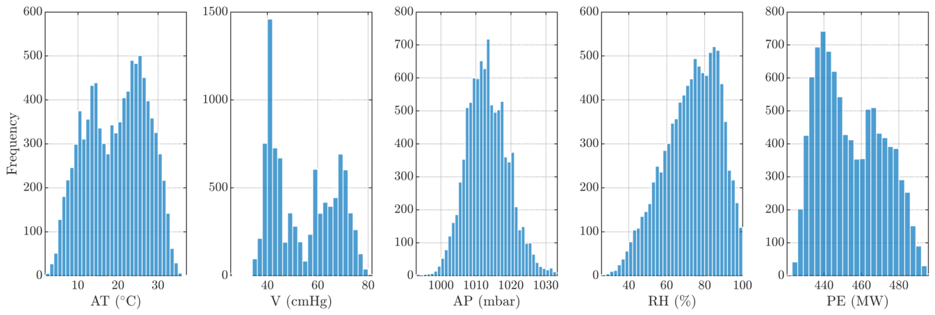
Figure 2. Kernel density estimates (PDFs) of the five CCPP variables: AT, V, AP, RH, and PE.

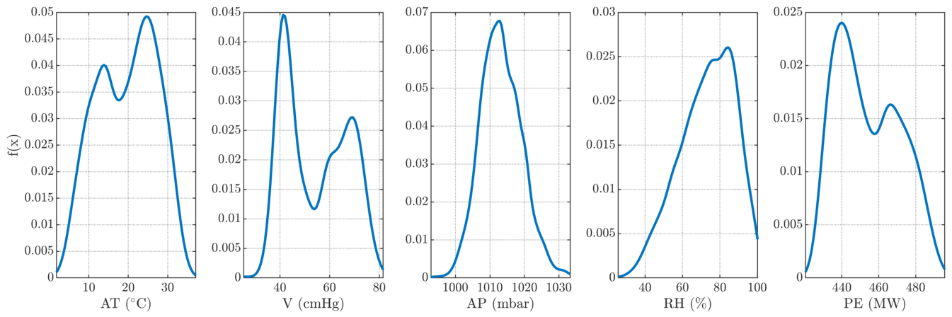
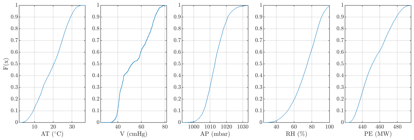
Figure 3. Empirical cumulative distribution functions (CDFs) of the five CCPP variables: AT, V, AP, RH, and PE.

Figure 3. Empirical cumulative distribution functions (CDFs) of the five CCPP variables: AT, V, AP, RH, and PE.

6.2. Implementation of the EERSS Design

Using the data, r sets of size $r+2$ are drawn, ranked, and the i-th ranked unit from each set is measured ($i=2,\dots ,r+1$), following the EERSS procedure of Section 3. This is repeated over c cycles to obtain the EERSS sample.

6.3. CDF Estimation and Comparison

For a set of representative points x, the estimators ${\widehat{F}}_{SRS}\left(x\right)$, ${\widehat{F}}_{RSS}\left(x\right)$, ${\widehat{F}}_{EERSS}\left(x\right)$, and ${\widehat{F}}_{MLE}\left(x\right)$ (with its confidence interval) are computed and compared, together with the relative efficiency of ${\widehat{F}}_{RSS}\left(x\right)$, ${\widehat{F}}_{EERSS}\left(x\right)$, and ${\widehat{F}}_{MLE}\left(x\right)$ with respect to ${\widehat{F}}_{SRS}\left(x\right)$.

Table 6. Summary statistics of the five CCPP variables ($N=9568$).

Variable	Mean	Median	SD	Min	Max	${\mathit{Q}}_1$	${\mathit{Q}}_3$	Skewness	Kurtosis
AT	19.65	20.35	7.45	1.81	37.11	13.51	25.72	−0.14	1.96
V	54.31	52.08	12.71	25.36	81.56	41.74	66.54	0.20	1.56
AP	1013.30	1012.90	5.94	992.89	1033.30	1009.10	1017.30	0.27	3.09
RH	73.31	74.98	14.60	25.56	100.16	63.33	84.83	−0.43	2.56
PE	454.37	451.55	17.07	420.26	495.76	439.75	468.43	0.31	1.95

Table 6. Summary statistics of the five CCPP variables ($N=9568$).

Variable	Mean	Median	SD	Min	Max	${\mathit{Q}}_1$	${\mathit{Q}}_3$	Skewness	Kurtosis
AT	19.65	20.35	7.45	1.81	37.11	13.51	25.72	−0.14	1.96
V	54.31	52.08	12.71	25.36	81.56	41.74	66.54	0.20	1.56
AP	1013.30	1012.90	5.94	992.89	1033.30	1009.10	1017.30	0.27	3.09
RH	73.31	74.98	14.60	25.56	100.16	63.33	84.83	−0.43	2.56
PE	454.37	451.55	17.07	420.26	495.76	439.75	468.43	0.31	1.95

Table 7, Table 8, Table 9 and Table 10 compare the empirical and MLE estimators of $F\left(x_0\right)$ under SRS, RSS and EERSS, for all five CCPP variables at $r=4$, $c=30$. SRS has the smallest bias in most rows, as expected since it is exactly unbiased; the EERSS MLE corrects this almost entirely, while the empirical EERSS estimator carries a large bias away from the median, confirming Theorem 3.1. In MSE, the EERSS MLE is the smallest in every single row, since it combines a small bias with a low variance. This carries directly into relative efficiency: the EERSS MLE gives the largest RE in every case, reaching as high as $3.20$ at the median, while the empirical EERSS estimator falls well below SRS in the tails. The average estimates mirror the bias results, with SRS and the EERSS MLE closest to the true $p_{\mathrm{true}}$ in most rows. These patterns hold consistently across all five variables.

7. Conclusion

This paper developed estimators of the CDF under the EERSS design. We derived the empirical CDF estimator in closed form and showed that it is biased in general, becoming exactly unbiased only at the point where $F\left(x\right)=1/2$, regardless of the shape of the population; its bias, variance, and relative efficiency against SRS and RSS were all obtained numerically. We then built the MLE on the same binomial order-statistic structure, together with its Fisher information, asymptotic variance, and a confidence interval for $F\left(x\right)$. Putting both estimators through the same numerical comparison, exact for the empirical estimator and Monte Carlo for the MLE, and then checking them against a real dataset, tells one clear story. The maximum likelihood EERSS estimator is the one worth using: it is competitive with, and often better than, RSS near the centre of the distribution, while the plain empirical EERSS estimator carries a bias that no amount of extra data removes. RSS keeps the upper hand in the tails, regardless of which estimator is used there.

Future work could extend this framework to quantile estimation and to inference on other functionals of the CDF, such as reliability and hazard functions, under EERSS and its multistage extensions.

References

- Abdallah, M. S. (2022). Estimation of the population distribution function using varied L ranked set sampling. RAIRO – Operations Research, 56(2), 955–977. [CrossRef]
- Abu-Dayyeh, W. A., Samawi, H. M., & Bani-Hani, L. A. (2002). On distribution function estimation using double ranked set samples with application. Journal of Modern Applied Statistical Methods, 1(2), 443–451. [CrossRef]
- Abuhedary, M. Z. A., Khamnei, H. J., & Heydari, A. A. (2025). Evaluating stress-strength reliability estimation technique: A study on ranked set sampling for the Beta-Lomax distribution. Contemporary Mathematics, 6, 442–464. [CrossRef]
- Ahmad, S., Hussain, S., Al Mutairi, A., Kamal, M., Rehman, M. U., & SidAhmed Mustafa, M. (2024). Improved estimation of population distribution function using twofold auxiliary information under simple random sampling. Heliyon, 10(2), e24115. [CrossRef]
- Aldrabseh, M. Z., & Ismail, M. T. (2023). New modification of ranked set sampling for estimating population mean. Journal of Statistical Computation and Simulation, 93, 2843–2855. [CrossRef]
- Aldrabseh, M. Z., Ismail, M. T., & Al-Omari, A. I. (2024a). Double except extreme ranked set sampling for estimating population mean. Advances in Mathematical Modelling and Applications, 9, 415–430. [CrossRef]
- Aldrabseh, M. Z., Ismail, M. T., & Al-Omari, A. I. (2024b). Except-extremes ranked set sampling for estimating the population variance with two applications of real data sets. Austrian Journal of Statistics, 53, 99–113. [CrossRef]
- Aldrabseh, M. Z., Ismail, M. T., & Al-Omari, A. I. (2025). Enhanced estimation of strength-stress reliability using except extreme ranked set sampling under exponential distribution. Life Cycle Reliability and Safety Engineering. [CrossRef]
- Aldrabseh, M. Z., Rashedi, K. A., Atoom, A. A., Alshammari, T. S., & Al-Olaimat, N. M. (2025). Median augmented ranked set sampling for estimation of the population mean with applications to body health data. AIMS Mathematics, 10(12), 28954–28980. [CrossRef]
- Al-Nasser, A. D. (2007). L ranked set sampling: a generalization procedure for robust visual sampling. Communications in Statistics – Simulation and Computation, 36, 33–43. [CrossRef]
- Al-Odat, M. T., & Al-Saleh, M. F. (2001). A variation of ranked set sampling. Journal of Applied Statistical Science, 10, 137–146.
- Alomani, G., Benchiha, S. A., & Al-Omari, A. I. (2025). Estimation of the inverse power Lindley distribution parameters using ranked set sampling with an application to failure time data. Axioms, 14, 801. [CrossRef]
- Al-Omari, A. I., & Abdallah, M. S. (2023). Estimation of the distribution function using moving extreme and MiniMax ranked set sampling. Communications in Statistics – Simulation and Computation, 52(5), 1909–1925. [CrossRef]
- Al-Omari, A. I., Almanjahie, I. M., Hassan, A. S., & Nagy, H. F. (2020). Estimation of the stress-strength reliability for exponentiated Pareto distribution using median and ranked set sampling methods. Computers, Materials & Continua, 64, 835–857. [CrossRef]
- Al-Omari, A. I., & Haq, A. (2019). A new sampling method for estimating the population mean. Journal of Statistical Computation and Simulation, 89, 1973–1985. [CrossRef]
- Al-Omari, A. I., & Raqab, M. Z. (2013). Estimation of the population mean and median using truncation-based ranked set samples. Journal of Statistical Computation and Simulation, 83, 1453–1471. [CrossRef]
- Alsadat, N., Hassan, A. S., Elgarhy, M., Chesneau, C., & Mohamed, R. E. (2023). An efficient stress–strength reliability estimate of the unit Gompertz distribution using ranked set sampling. Symmetry, 15, 1–24. [CrossRef]
- Al-Saleh, M. F., & Al-Kadiri, M. A. (2000). Double-ranked set sampling. Statistics & Probability Letters, 48, 205–212. [CrossRef]
- Al-Saleh, M. F., & Al-Omari, A. I. (2002). Multistage ranked set sampling. Journal of Statistical Planning and Inference, 102, 273–286. [CrossRef]
- Asghari, S., Gildeh, B. S., & Ahmadi, J. (2018). Sign control chart based on ranked set sampling. Quality Technology & Quantitative Management, 15, 568–588. [CrossRef]
- Benchiha, S. A., Al-Omari, A. I., & Alomani, G. (2025). Enhanced estimation of the unit Lindley distribution parameter via ranked set sampling with real-data application. Mathematics, 13, 1645. [CrossRef]
- Chen, M., Chen, W. X., Yang, R., & Zhou, Y.W. (2025). Exponential–Poisson parameters estimation in moving extremes ranked set sampling design. Acta Mathematicae Applicatae Sinica, English Series, 41, 973–984. [CrossRef]
- David, H. A., & Nagaraja, H. N. (2003). Order statistics (3rd ed.). Hoboken, NJ: John Wiley & Sons. [CrossRef]
- Dong, X., & Zhang, L. (2020). Estimation of system reliability for exponential distributions based on L ranked set sampling. Communications in Statistics – Theory and Methods, 49, 3650–3662. [CrossRef]
- Farah, M. N., & Hanif, F. A. M. (2021). Modified extreme ranked sets sampling with auxiliary variable. Proceedings of the National Academy of Sciences, India, Section A: Physical Sciences, 91, 537–542. [CrossRef]
- Frey, J., & Zhang, Y. (2023). Nonparametric maximum likelihood estimation of the distribution function using ranked-set sampling. Journal of the Korean Statistical Society, 52(4), 901–920. [CrossRef]
- Halake, K. S., Godase, D. G., & Mahadik, S. B. (2020). Power comparison of Kolmogorov-Smirnov test under ranked set sampling and double ranked set sampling. International Journal of Agricultural and Statistical Sciences, 16(2), 671–677.
- Haq, A. (2016). Estimation of the distribution function under hybrid ranked set sampling. Journal of Statistical Computation and Simulation, 87(2), 313–327. [CrossRef]
- Haq, A., Brown, J., Moltchanova, E., & Al-Omari, A. I. (2016). Paired double-ranked set sampling. Communications in Statistics – Theory and Methods, 45, 2873–2889. [CrossRef]
- Hassan, A. S., Metwally, D. S., Semary, H. E., Benchiha, S. A., Gemeay, A. M., & Elgarhy, M. (2025). Improved estimation based on ranked set sampling for the Chris–Jerry distribution with application to engineering data. Computer Journal of Mathematics and Statistics Science, 4, 424–456. [CrossRef]
- Kaya, H., Tüfekci, P., & Gürgen, S. F. (2012). Local and global learning methods for predicting power of a combined gas & steam turbine. In Proceedings of the international conference on emerging trends in computer and electronics engineering (icetcee) (pp. 13–18). Dubai.
- Khan, L., Shabbir, J., & Khalil, U. (2019). A new systematic ranked set-sampling scheme for symmetric distributions. Life Cycle Reliability and Safety Engineering, 8, 205–210. [CrossRef]
- Kumar, A., Bhushan, S., & Pokhrel, R. (2025a). Direct and synthetic logarithmic estimators in small area estimation via ranked set sampling. Statistics, 1–22. [CrossRef]
- Kumar, A., Bhushan, S., & Pokhrel, R. (2025b). Small area estimation under ranked set sampling: simulation and real-life application with crop production data. Quality & Quantity, 1–21. [CrossRef]
- Mahdizadeh, M., & Zamanzade, E. (2022). CDF estimation in multistage pair ranked set sampling. Hacettepe Journal of Mathematics and Statistics, 51(6), 1768–1779. [CrossRef]
- McIntyre, G. A. (1952). A method for unbiased selective sampling using ranked sets. Australian Journal of Agricultural Research, 3, 385–390. [CrossRef]
- Mohammadkhani, A., Amiri, A., & Khoo, M. B. C. (2023). A review of ranked set sampling and modified methods in designing control charts. Quality and Reliability Engineering International, 39, 1465–1493. [CrossRef]
- Muttlak, H. A. (1997). Median ranked set sampling. Journal of Applied Statistical Science, 6, 245–255.
- Obeidat, M., Na’amneh, R. M., Hanandeh, A. A., Aldrabseh, M. Z., & Omara, T. M. (2026). A new ranked set sampling design for estimating population mean and variance based on neoteric ranked set sampling. Journal of the Nigerian Society of Physical Sciences, 3529. [CrossRef]
- Obeidat, M., Namneh, R., Hanandeh, A., & Rawashdeh, A. (2025). New highly efficient one and two-stage ranked set sampling variations. Pakistan Journal of Statistics and Operation Research, 163–176. [CrossRef]
- Samawi, H. M., & Al-Sagheer, O. A. M. (2001). On the estimation of the distribution function using extreme and median ranked set sampling. Biometrical Journal, 43(3), 357–373. [CrossRef]
- Sevil, Y. C., & Yildiz, T. O. (2017). Power comparison of the Kolmogorov–Smirnov test under ranked set sampling and simple random sampling. Journal of Statistical Computation and Simulation, 87(11), 2175–2185. [CrossRef]
- Sevil, Y. C., & Yildiz, T. O. (2022). Design-based estimators of the distribution function in ranked set sampling with an application. Statistics, 56(4), 891–918. [CrossRef]
- Sevil, Y. C., & Yildiz, T. O. (2023). Estimation of distribution function using percentile ranked set sampling. REVSTAT – Statistical Journal, 21(1), 39–62. [CrossRef]
- Shehzada, M. A., Nisara, A., Khana, A., Emamb, W., Tashkandyb, Y., & Khurram, H. (2024). Modified median quartile double ranked set sampling for estimation of population mean. Heliyon, 10, e34627. [CrossRef]
- Stokes, S. L., & Sager, T. W. (1988). Characterization of a ranked-set sample with application to estimating distribution functions. Journal of the American Statistical Association, 83(402), 374–381. [CrossRef]
- Takahasi, K., & Wakimoto, K. (1968). On unbiased estimates of the population mean based on the sample stratified by means of ordering. Annals of the Institute of Statistical Mathematics, 20, 1–31. [CrossRef]
- Tüfekci, P. (2014). Prediction of full load electrical power output of a base load operated combined cycle power plant using machine learning methods. International Journal of Electrical Power & Energy Systems, 60, 126–140. [CrossRef]
- Yildiz, T. O., & Sevil, Y. C. (2018). Performances of some goodness-of-fit tests for sampling designs in ranked set sampling. Journal of Statistical Computation and Simulation, 88(9), 1702–1716. [CrossRef]
- Yildiz, T. O., & Sevil, Y. C. (2019). Empirical distribution function estimators based on sampling designs in a finite population using single auxiliary variable. Journal of Applied Statistics, 46(16), 2962–2974. [CrossRef]
- Yu, P. L. H., & Lam, K. (1997). Regression estimator in ranked set sampling. Biometrics, 53, 1070–1080. [CrossRef]
- Zamanzade, E. (2019). EDF-based tests of exponentiality in pair ranked set sampling. Statistical Papers, 60(6), 2141–2159. [CrossRef]
- Zamanzade, E., & Mahdizadeh, M. (2020). Using ranked set sampling with extreme ranks in estimating the population proportion. Statistical Methods in Medical Research, 29(1), 165–177. [CrossRef]
- Zamanzade, E., Mahdizadeh, M., & Samawi, H. M. (2020). Efficient estimation of cumulative distribution function using moving extreme ranked set sampling with application to reliability. AStA Advances in Statistical Analysis, 104(3), 485–502. [CrossRef]
- Zamanzade, E., & Wang, X. (2018). Proportion estimation in ranked set sampling in the presence of tie information. Computational Statistics, 33(3), 1349–1366. [CrossRef]
- Zhang, W., Zhu, X., He, M., & Narayanaswamy, B. (2025). Reliability test for degradation data based on ranked set sampling. Quality and Reliability Engineering International, 41, 235–254. [CrossRef]