

Submitted:
13 October 2026
Posted:
14 October 2026
You are already at the latest version
Abstract
In artificial-intelligence-of-things (AIoT) deployments, fleets of heterogeneous, long-lived sensing devices sit behind an edge tier whose cloud is not always reachable, so a device trusted at enrolment must be re-assessed continuously, with a response it can afford and with knowledge shared across sites. We present EASA, an Edge-centric Adaptive Security API: a gateway fuses per-flow anomaly evidence with each device’s reported posture and decision history into a composite trust score, maps it with hysteresis to four persistent enforcement levels, budgets the step-up action by the device’s reported energy, and uses a cloud security service only for cross-gateway state—a federated detector and a credential-revocation registry. Every component can be disabled, so baselines are configurations of one implementation. We evaluate the prototype on per-address traces of 65 real consumer devices (CIC IoT-DIAD 2024) under synthetic campaigns built from weakly labelled attacker traces, with three emulated gateways and a cloud service deployed on Google Cloud Run, all calibrated to one target false-positive rate. Over 30 paired seeds, federated aggregation raised recall on attack families unseen at a gateway from 0.24 to 0.60, the shared registry caught 81% of credential-replay device-epochs across all runs, the full EASA configuration isolated about 45% fewer clean devices than per-alarm blocking, the energy-aware selector performed 37% fewer re-authentications under simulated low battery, and a 15-minute cloud outage after warm-up reduced replay rejection with no change detected in the evaluated local metrics (103 ms mean per-run median round trip); the composite score’s history term, in contrast, prolonged benign-side restriction without a demonstrated detection gain. The released simulator, cloud service and protocol give AIoT operators and API designers a reproducible basis for graded, resource-aware enforcement at the edge.
Keywords:
AIoT
; edge computing
; security API
; zero trust
; cloud security service
1. Introduction
Sensing devices that carry their own inference—cameras, pre-processing sensors, hubs fusing telemetry from dozens of nodes—are now deployed in numbers that make per-device security management impractical. These AIoT fleets stress security designs inherited from enterprise networks: heterogeneous capability makes one cryptographic policy too heavy for a battery-powered sensor or too weak for a mains-powered camera; long lifetimes and rare patching mean a device trustworthy at enrolment may not be a year later; and the edge tier is itself a target [1,2], while cloud latency and intermittent availability exclude the cloud from the time-critical decision path considered here [3].
Recent threat-intelligence reports describe AI-assisted reconnaissance and agentic workflows for vulnerability scanning and credential harvesting [4,5]. For API-mediated AIoT deployments, these observations reinforce the need to reassess the privileges of authenticated devices and to propagate credential revocations across sites, motivating continuous enforcement that responds locally under device-resource and connectivity constraints. The experiments in this paper evaluate that control loop through scripted trace replay; autonomous AI-agent attacks and application-level API vulnerabilities are outside the evaluated scope.
The literature has moved security to the edge and made it adaptive: gateways externalising authentication and intrusion prevention [6], zero-trust admission control that scores every message and can accept, challenge or revoke [7], learned trust with resource-stress evidence gating federated task placement [8] and machine-learning detection of zero-trust violations at the 5G edge [9]. Read together, they leave three gaps. First, the enforcement a trust or risk value triggers is per message or per task, binary (admit, block) or outside the evaluated system; a persistent, graded per-device security state, stepped up and relaxed with hysteresis, is not evaluated, although it follows the continuous-evaluation principle of zero-trust architecture [10,11]. Second, the device’s own state (energy, compute headroom, link quality, firmware integrity), already reported for its own management, enters these designs, if at all, as evidence of suspicion or a scheduling constraint rather than as a budget for the response—what is needed to decide how to respond to a suspicious device without draining a legitimate one. Third, the cloud is absent or only an analytics back-end, so the functions at which a single gateway is weakest—detecting an attack family another site has seen and rejecting a credential revoked elsewhere—are not measured, nor is the cost of reaching a real cloud service.
This paper presents the Edge-centric Adaptive Security API (EASA): an edge gateway exposes a small set of security primitives to devices and cloud services and continuously re-negotiates each device’s security level from a composite trust score fusing a per-flow anomaly detector’s output with the device’s reported posture and decision history. A policy decision point maps the score, with hysteresis, to four enforcement levels from normal operation to quarantine, and a cloud service holds the state shared across gateways—an aggregated detector, versioned policy, a revocation registry—without being in the decision path. Every component can be disabled, so the baseline comparison is an internal ablation, not a re-implementation contest.
We evaluate EASA as a system prototype on the flow-based release of the CIC IoT-DIAD 2024 dataset [12,13], replaying per-address traces of 65 real consumer devices of the CIC testbed under synthetic attack campaigns against three emulated gateways and a cloud service on Google Cloud Run in the Seoul region, so every cross-gateway interaction incurs a real round trip. As the release is not labelled per flow, we release a transparent row-level labelling rule and state its limits; as configurations that compute trust differently sit at different operating points for one threshold, we calibrate each to the same target false-positive rate on a benign segment preceding the evaluated one before comparing recall, containment and overhead. The contributions are:
- An edge-centric security architecture whose API contract, composite trust score, state-transition rules and four-level policy are specified so that baselines inspired by four design classes—static authentication, gateway virtual security functions, rule-based zero-trust admission and network-only learned trust—are configurations of the same implementation, with evaluated, emulated and specified-only parts stated (Section 3).
- A reproducible evaluation protocol on IoT-DIAD 2024: row-level labelling with disclosed attacker sets, device-level trace replay, forced cross-site and credential-replay campaigns, operating-point calibration at a fixed target false-positive rate, and metrics with stated units and denominators (Section 4).
- Evidence over 30 paired seeds, at a common target false-positive rate on clean devices, that the cloud’s federated model raises recall on attack families a gateway never saw, but another site had, from 0.24 to 0.60, and its revocation registry catches 81% of credential-replay epochs over all runs (85% when a revocation exists), a family a local detector catches only by coincidence; that the full configuration restricts more attack episodes than the per-alarm configuration with a stronger detector while isolating about 45% fewer clean devices (4.2% vs. 7.7%; a whole-configuration trade-off); that the energy-aware action selector, isolated with everything else held equal, performs 37% fewer re-authentication handshakes in a low-battery scenario with no detected change in detection or restriction metrics; and the negative results that the composite trust score, with the cloud held constant, does not demonstrate an improvement on any detection metric and lengthens benign-side restriction—a lock-in that a trajectory audit traces to the decaying history term and that a history reset reduces but does not remove—that the graded loop is not faster than per-alarm blocking, and that a stronger per-flow detector detects in-distribution attacks better (Section 5).
- A measured account of the real cloud path: 596 calls per run at a 103 ms mean per-run median round trip in the main EASA runs, zero failures across the 270 cloud-dependent runs, per-seed metrics identical to those of an in-process mock, and a 15-minute outage after warm-up that reduces replay rejection with no change detected in the evaluated local metrics (Section 5.5 and Section 5.8).
The paper is organised as follows. Section 2 (Related Work) analyses lightweight authentication, edge-externalised security, zero-trust and learned trust at the edge, federated learning and their evaluation datasets, and positions EASA against the closest designs. Section 3 (Proposed Architecture: Edge-Centric Adaptive Security API (EASA)) describes the architecture. Section 4 (Experimental Setup) describes the data, emulation, calibration and baselines. Section 5 (Experimental Results) presents the results. Section 6 (Discussion) analyses their limits and practical implications. Section 7 (Conclusions) concludes. The simulator, labelling rule, cloud service and all configuration files are released with the paper.
2. Related Work
We group prior work by the question it answers—device authentication, security externalised to the edge, trust assessment, the cloud’s contribution—and close with the datasets that make such systems comparable. Table 1 aligns the closest designs on the four axes our evaluation measures.
2.1. Lightweight Authentication for Cloud-Connected IoT
Lightweight authentication and key agreement for constrained devices—three-party authentication for cloud-connected services [14], provably secure mutual authentication for cloud-based IoT [15], elliptic-curve protocols with tracking-resistant dynamic credentials [16]—decides whether a device may join. Such protocols are verified against protocol-level adversaries and costed by computation and communication, which the handshake dominates on constrained nodes; the DTLS measurements of Raza et al. [17] are why EASA treats a re-handshake as a costed action, not a free check. By design they are blind to what a device does after joining: a compromised device with valid credentials passes every check. EASA does not replace them—its step-up invokes whichever handshake the device class supports—but adds the continuous assessment that decides when the handshake is worth its cost. Static authentication is baseline B0.
2.2. Security Externalised to the Edge
Many devices cannot run security functions at all, so a second line moves them to a gateway. The IoT Proxy [6] externalises a static chain of virtual network security functions (VPN termination, a machine-learning intrusion prevention system) that protects resource-limited devices transparently: an IPS alarm blocks the flow, and a device’s posture does not change with evidence. Two earlier gateways, the nearest precedents of our enforcement tier, keep a per-device restriction state. IoT SENTINEL [18] fingerprints the device type from enrolment traffic, looks it up in a vulnerability database and assigns one of three gateway-enforced isolation classes (strict, restricted, trusted), with policy cached at the gateway and refreshed periodically from a remote server; its Raspberry Pi gateway evaluation measures traffic latency to local and remote servers, including an Amazon EC2 endpoint. IoT-KEEPER [19] detects malicious activity with a fuzzy-clustering classifier over flow features and moves the offending device, by link-layer address, into one of three overlay networks (no access, restricted, full) via software-defined flow rules; analysis runs on the gateway, policies and trained rules are described as shareable across gateways, and the evaluation is a Raspberry Pi testbed with real devices. Neither specifies or evaluates the trust-threshold, hysteresis-based bidirectional controller studied here (IoT-KEEPER describes policy-cache expiry and overlay-network updates; otherwise a class is set at identification or at detection), budgets the response by the device’s reported resources, or evaluates the cross-site functions—a shared detector and a shared revocation list—against a deployed service with measured round trips. EASA adds that closed loop (a graded level stepped up and relaxed over time with hysteresis from a continuously updated trust value, an action selector conditioned on reported energy, separately measured cloud functions) but, unlike both, is not evaluated on gateway hardware. Realguard [20] couples a gateway intrusion detector to an action manager that logs, notifies or blocks, so gateway detection-to-response coupling is established; open is the shape of the response state. A patent [21] describes, without a published evaluation, a gateway that periodically summarises device interactions, receives a cloud signature and flags deviations. The IoT Proxy’s per-alarm blocking inspires baseline B1; what the gateway should do between “allow” and “block” is the subject of our four-level policy.
2.3. Zero Trust and Learned Trust at the Edge
Zero-trust architecture [10] prescribes continuous evaluation of every access and a policy engine acting on it; surveys [11,22] find that engine its least specified component, and its IoT transfer has been argued as principles for non-human identities [23] and surveyed across cloud, edge and fog [1,2,24]. IoT trust management is older: Yan et al. [25] classify trust by the properties it aggregates, Chen et al. [26] combine direct observation with recommendation and decay it over time (the pattern of our decision-history term), and ledger-backed trust is surveyed in [27]; these models rarely specify the enforcement a trust value triggers, our question here. Dimitrakos et al. [28] formulated trust-aware continuous authorization for consumer IoT, and Jeong and Yang [29] select allow, additional authentication or block from a weighted trust score over user behaviour, network environment, device status and threat history, reassessed during a session; EASA builds on this established score-to-policy pattern. YB-IoT-CG [7] screens each authenticated message with a deterministic, policy-based risk score over freshness (nonce, timestamp), gateway-observed context and firmware-state evidence, answers Accept, Challenge or Revoke per message, anchors confirmed revocations on a permissioned ledger with an on-chain registry, and is evaluated by packet-level simulation on synthetic traffic. EdgeGuard-AI [8] keeps a per-node trust value with exponential forgetting from flow statistics (bursts, flag behaviour, anomaly concentration) and resource-stress indicators (CPU, memory, queue pressure); trust gates which nodes receive sensitive tasks under a risk budget, with federated averaging at the server, so trust selects where work is placed, resource stress is evidence of suspicion, and what remaining energy should change about the response is not modelled. Ashfaq et al. [9] predict zero-trust violations at the 5G edge with machine learning on CICDDoS2019 in an SDN emulation; the loop closes at detection. Aydin’s federated multi-agent defence (FMAD) for edge–cloud IoT [30] validates only the threat-intelligence agent empirically; the mitigation agent remains at design level.
EASA evaluates what this set lacks: a persistent, graded per-device security level with explicit escalation and release rules (YB-IoT-CG decides per message, EdgeGuard-AI gates placement), stepped up and relaxed over time with hysteresis; the device’s reported resource posture as a budget for the response (EdgeGuard-AI reads resource stress as evidence, but neither design lets a low battery change which enforcement action is taken); and cross-gateway model and revocation services. The first two cost one posture beacon per epoch and one bit per past decision, and Section 3.3 and Section 3.4 make the case that both change the right enforcement action.
2.4. Federated Learning and the Role of the Cloud
Federated learning shares detector knowledge across sites without sharing traffic [31,32]. For IoT intrusion detection, Rahman et al. [33] compare centralised, on-device and federated training, finding federated detectors close to centralised ones on non-IID NSL-KDD partitions; Mothukuri et al. [34] federate a recurrent detector over device traffic; DÏoT [35] established federated, device-type-specific anomaly detection across local security gateways; Nguyen et al. [36] show that compromised IoT devices can poison the training traffic of otherwise uncompromised federated gateways; and partitioned IIoT data has been federated [37]. In all of these the cloud is an aggregator and the quantity of interest is model accuracy. Unmeasured are what a federated model does for the security policy of a gateway that has never seen a given attack family, and the second cross-site function—propagating one gateway’s revocation to the others—for which blockchain ledgers have been proposed [7]. We treat both as first-class cloud functions, evaluate them against a real deployment, and quantify what is lost when the cloud is unreachable.
2.5. Datasets and Evaluation Practice
Comparable evaluation depends on shared data used without the closed-world assumptions Sommer and Paxson [38] warned against; Ring et al. [39] catalogue the available network datasets and their recurring labelling and representativeness problems. Consumer IoT traffic is sparse and periodic with few endpoints per device [40], which makes device-level replay meaningful and lets a gateway identify device types [18]; the Mirai family dominating IoT botnet datasets is described in [41]. CICIoT2023 [42] provides 33 attacks in seven classes from a testbed of 105 real devices; its flow-based 2024 re-release, IoT-DIAD [12,13], adds endpoints and timestamps to every flow, enabling device-level replay. TON_IoT [43] and Edge-IIoTset [37] add telemetry and multi-tier captures. Two cautions shaped our protocol: Purkaystha et al. [44] report that a naive Bot-IoT split in their study contained up to 97% duplicate rows and that zero-day performance must be measured on families held out of training, both of which we adopt; and threat-model studies of sensing systems [45] argue for explicit trust zones across sensor, edge and cloud, which our system model follows.
2.6. Positioning
In Table 1, “graded” means more than two persistent enforcement levels per device and “deployed cloud” a service reached over the Internet with measured round trips; detection-only designs such as [9] are omitted because they do not enforce at all. Graded per-device isolation at a gateway is not new—IoT SENTINEL and IoT-KEEPER both assign a device to one of three classes—and score-to-policy control with session reassessment is established [29]. What this study contributes is an API-based integration and a controlled trace-replay evaluation of persistent device-level restriction, resource-conditioned response selection, and shared model and revocation services, quantifying their detection and restriction-cost trade-offs with a measured cloud path; no design in this set evaluates that combination, and because each is evaluated in its own environment, their numbers cannot be compared with one another. We do not claim to reproduce these designs: the baselines of Table 5 are configurations of EASA inspired by selected design classes of the table—selected traits (detector family, binary or graded enforcement, cloud functions used), implemented once in our simulator and run on the same traces at the same target operating point—and are internal ablations standing in for a design class, not re-implementations of a particular paper or reproductions of its reported performance.

Table 1.
Closest designs on the four axes measured in this paper, summarised from the cited papers.
| Work | Trust input | Enforcement | Cloud role | Evaluation |
|---|---|---|---|---|
| Lightweight AKA [14,15,16] | credentials only | admit at join | key/registration server | protocol cost, formal proof |
| IoT Proxy [6] | IPS alarm | allow / block | none | testbed throughput |
| IoT SENTINEL [18] | device-type fingerprint + vulnerability database | three isolation classes, assigned at identification | policy server (cached, refreshed) | Raspberry Pi gateway; traffic latency to local and remote servers incl. an EC2 endpoint |
| IoT-KEEPER [19] | fuzzy-clustering anomaly score on flow features | three overlay networks per device, assigned at detection | none in the evaluation (policy sharing described) | Raspberry Pi testbed, real devices, accuracy and overhead |
| YB-IoT-CG [7] | deterministic risk score: freshness, context, firmware evidence | per-message Accept / Challenge / Revoke | ledger-anchored revocation registry | packet-level simulation, synthetic traffic |
| Trust-score ZTA [29] | weighted score: user behaviour, network, device status, threat history | allow / additional authentication / block, reassessed in session | policy server | real-world performance evaluation |
| EdgeGuard-AI [8] | learned trust from flow statistics + resource stress | binary admissibility gate for task placement | federated aggregation server | replay of Edge-IIoTset flows |
| FMAD [30] | threat-intelligence agent | designed, not evaluated | federated agents | detector only, CIC-IoT-2023 |
| EASA (this paper) | network + reported posture + decision history | four persistent graded levels; posture budgets the action | federated model + revocation registry, outside the decision path | replay of IoT-DIAD 2024 device traces, deployed cloud (Cloud Run, Seoul), ablation at a fixed target FPR |
3. Proposed Architecture: Edge-Centric Adaptive Security API (EASA)
In the Edge-centric Adaptive Security API (EASA) an edge gateway exposes a small, stable set of security API primitives to AIoT devices and cloud services and continuously re-negotiates each device’s security posture from a composite trust score. Its design goals follow from the gaps of Section 2:
- G1
- G2
- G3
- Resource-aware adaptation. Device resource posture (energy, compute headroom, link quality) is an explicit input to the trust model, not merely a deployment constraint [23].
- G4
- Cloud as a first-class participant. The cloud layer owns the global trust model, cross-gateway threat correlation, policy distribution and revocation—functions that no single edge node can perform alone [24].
- G5
- Comparability. Every component of the composite score and of the cloud path can be disabled, so that baselines inspired by the published designs of Section 2 are configurations of the same implementation (Section 3.8).
3.1. System Model and Threat Model
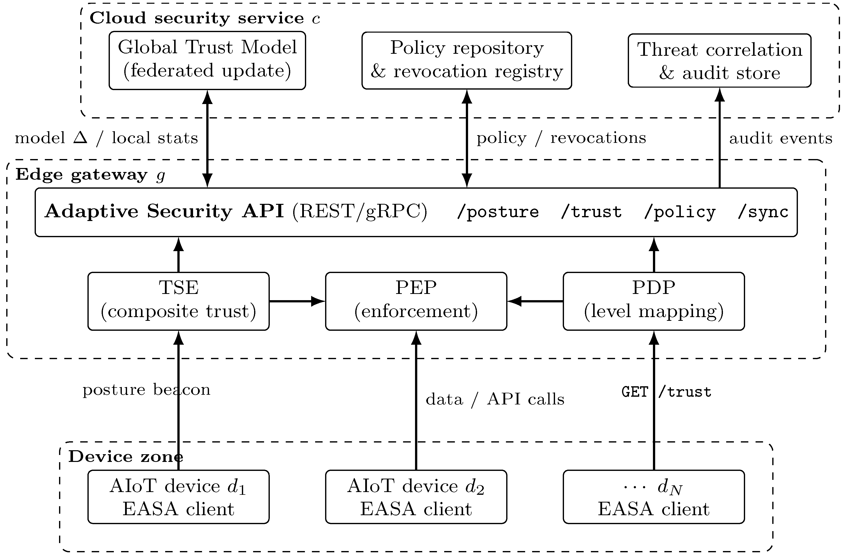
Entities. Devices attach to a gateway g; a cloud security service c serves gateways . A lightweight EASA client on each device emits a periodic posture beacon; the gateway hosts the Trust Scoring Engine (TSE), Policy Decision Point (PDP) and Policy Enforcement Point (PEP); the cloud hosts the Global Trust Model (GTM), policy repository, revocation registry and audit store (Figure 1).
Trust zones. Adapting the STRIDE-based zoning of [45] to three tiers, three trust zones (device, edge, cloud) are separated by two boundaries (local wireless link, Internet uplink); cross-boundary traffic is mutually authenticated (mTLS or DTLS-PSK by device class; the prototype of Section 4 uses an API key over HTTPS at the gateway–cloud boundary).
Adversary. The adversary may (i) compromise a legitimate device and use it to launch volumetric or reconnaissance attacks (botnet enrolment), (ii) spoof or replay device credentials, (iii) tamper with sensing payloads, and (iv) attempt lateral movement toward the gateway. The adversary cannot break standard cryptographic primitives and does not control the cloud service. We explicitly include a compromised device that keeps valid credentials, to which static authentication [14,15] is blind, and that may lie in its posture beacon (signing proves the sender, not the contents). EASA therefore treats the beacon’s resource fields as self-reported and bounds their influence (Section 3.3), and takes the integrity flag from an attestation mechanism outside the API (measured boot or remote attestation verified by gateway or cloud, not the device); in the evaluation that flag is an oracle, so the firmware-tampering results measure the policy’s response, not the attestation.
3.2. Architecture Overview
All adaptation decisions are taken at the edge within a bounded latency budget; the cloud improves them asynchronously. A gateway cut off from the cloud degrades gracefully, scoring and enforcing with its last synchronised model and policy and queueing audit events for later upload.
Figure 1.
EASA architecture: the gateway closes the sense–score–decide–enforce loop locally and the cloud holds only cross-gateway state.
Figure 1.
EASA architecture: the gateway closes the sense–score–decide–enforce loop locally and the cloud holds only cross-gateway state.
3.3. Composite Trust Score
For device d at epoch t the TSE fuses three normalised sub-scores in into a composite trust score .
Network behaviour score . A lightweight per-flow classifier (a two-layer multilayer perceptron, chosen because its parameters can be averaged across gateways; any per-flow classifier can be substituted) maps each flow to an attack probability . With the flows of d in the window of length W ending at t, the window score is a top-k mean,
where are the k highest-probability flows and missing terms are zero when the window holds fewer than k flows (an empty window gives ). This soft evidence pooling caps one confident alert at : a single benign false alarm cannot dominate a sparse window, several alerts within W accumulate, and it is not a count rule (two alerts at probability 1 give with , which may or may not cross the calibrated threshold, Section 4.5). is initialised from the GTM, which federated-averages the gateways’ locally trained parameters (Section 3.6).
Device posture score . From the beacon we take energy headroom , compute headroom and link quality , each clipped to , and an integrity flag from the attestation mechanism (firmware measurement matches the registry):
A failed integrity check drives to zero irrespective of resources. Because are self-reported, the posture term contributes at most to the instantaneous fused score . This bounds its direct additive contribution, but it does not guarantee resistance to evasion through a falsified posture: near a threshold, the difference between a truthful low posture and a forged healthy one (up to ) can decide whether is entered, and a device that under-reports its energy can obtain the deferral of the re-handshake, although rate limiting and scope reduction still apply. Such resistance was not evaluated (Section 6.3). The PDP also consumes posture when selecting the enforcement action, so a low-energy benign device is not pushed into a costly re-authentication loop (G3).
Decision history . An exponentially weighted record of the policy’s own past decisions,
where is the previous level (Table 2) and controls memory. The decay follows the reputation models of [25,26], but the evidence is the policy’s own decision, so this is policy memory, not independent evidence: a recently restricted device recovers gradually, not at the first clean window, and one oscillating around a threshold settles at the stricter level. The price, a slower return to after a false alarm, is measured (post-attack dwell, restricted share of benign epochs; Section 5.1) and bounded analytically in Section 3.4.
Fusion and smoothing.
Here sum to one, , and (a new device is trusted until evidence accrues). Weights and are policy parameters, possibly per device class. The defaults (, ) encode two design decisions, not a fit to the test data: network evidence is the only term that can detect an attack, so it must carry a device across the restriction threshold alone (); posture and history are regularisers whose combined weight should separate a clean record from none, while the bound limits the direct weighted contribution of a forged posture to (Section 3.1); it does not by itself guarantee that a forged posture cannot keep a device above a calibrated threshold, and resistance to such evasion is not verified in this paper. Whether the regularisers add detection value at a fixed operating point is an empirical question, answered negatively for this formulation in Section 5.1; Appendix C varies over . Setting recovers a purely network-driven trust model in the spirit of [8], and replacing with a deterministic screen in the spirit of [7] a rule-based score; these reductions underlie Section 3.8.
3.4. Security Levels and Policy Decision
The PDP maps to four discrete security levels with hysteresis (Table 2): promotion to a stricter is immediate when ; relaxation requires for h consecutive epochs. The thresholds fix the operating point and are set from the benign distribution of to meet a target false-positive rate (Section 4.5).
Table 2.
Security levels enforced by the PEP (each level applies its actions in addition to those of the levels below it).
Table 2.
Security levels enforced by the PEP (each level applies its actions in addition to those of the levels below it).
| Level | Trust band | Enforcement actions (PEP) |
|---|---|---|
| Normal | Default token TTL; baseline telemetry rate; full API scope. | |
| Observe | Token TTL halved; telemetry rate ; audit event to cloud; no user-visible change. | |
| Restrict | Step-up re-authentication (mTLS re-handshake or challenge); per-device rate limit; API scope reduced to read-only / essential endpoints; cloud notified for cross-gateway correlation. | |
| Quarantine | or | Traffic dropped at PEP; credential pushed to cloud revocation registry; neighbouring gateways alerted; manual or policy-timed release. |
Posture modulates which action is chosen: below an energy floor the PDP prefers rate limiting and scope reduction to cryptographic step-up and marks the re-handshake pending; it executes at the first later epoch at which the device is still at or stricter with above the floor, and is cancelled if the device first relaxes to or (rate limit and scope reduction having been lifted). This is how resource awareness changes behaviour (G3) rather than merely being measured.
State transitions and recovery. Table 3 makes the transition rules explicit, one row per case, including the cases Algorithm 1 handles when the level does not change; in the table ℓ is the previous level, T the current trust, the exit threshold of , and “Action” the one-shot action issued in that epoch in addition to the level’s standing enforcement (Table 2), “none” being the default when nothing changes. Three properties matter for the evaluation. (i) Promotion is immediate and driven by , or the revocation cache; relaxation is one level at a time and requires to exceed the exit threshold for h consecutive epochs. (ii) Every entry into publishes a revocation, and a revoked or tampered credential holds the device at while the revocation is in force; the policy-timed release of Table 2 applies only to a credential that has been reinstated. Re-enrolment after a quarantine (new credential, registry update) is an operator action outside the API and is not modelled, so in the evaluation is absorbing within a run. (iii) Because decays while a device is restricted, a device at can only recover if its other evidence suffices without history: asymptotically, requires , with in the worst case. With the calibrated thresholds of Section 5.9 () and the default weights, a benign device recovers whenever its window score satisfies , i.e. for a mains-powered device () and for a sensor node at 60% charge (). The condition is not guaranteed: a benign device whose traffic the detector finds persistently suspicious, or whose reported resources are low (with and a clean network score the asymptotic fused score is ), can remain at until an operator intervenes, and the policy provides no finite recovery guarantee. We report the observed restricted share of benign epochs and the post-attack dwell (Section 5.1) and audit the saved trajectories for benign devices still restricted at the end of a run (Section 5.7), which finds exactly this lock-in. A history reset after h consecutive epochs with a clean network score at removes the dependence; it was not part of the pre-specified protocol and is evaluated as a supplementary revision.
3.5. Adaptive Security API
The API is deliberately small (Table 4); devices use only the first group and the cloud sees only the last. Cloud calls carry a model version for drift detection; repeating a revocation or model push with the same version has no further effect (idempotent), whereas a repeated audit event is stored twice and de-duplicated by event identifier at analysis time. In Table 4, D, E and C denote the device, the edge gateway and the cloud; the frequencies are design defaults, which the evaluation compresses for the cloud intervals (Section 4.6); and the last column states, for each primitive, whether it is exercised over HTTPS against the deployed service in the evaluation of Section 5 (net), emulated in-process in the simulator (emu), or specified but not implemented (spec).
Three device-facing endpoints fit a constrained-device footprint; a posture beacon is a few dozen bytes and can piggyback on an MQTT keep-alive.
3.6. Role of the Cloud Layer
Three functions are impossible at a single gateway. The global trust model and revocation registry are implemented in the deployed service and evaluated; policy distribution is specified and, in the evaluation, replaced by the per-run calibration of Section 4.5; the audit store is an event sink only—cross-gateway correlation on its contents is a design goal (G4) that we do not evaluate.
- Global Trust Model. Each gateway trains on local traffic from a common initialisation and uploads its parameters; once all have pushed, the cloud computes a sample-weighted federated average [31] and redistributes with a new version, so an attack family first seen at raises sensitivity at before it is attacked (evaluated as cross-site generalisation, Section 5).
- Policy distribution. Weights, thresholds and hysteresis parameters are versioned in the cloud; operators tune a device class once and all gateways converge within one sync period.
- Revocation and correlation. An event publishes the credential to the registry; other gateways pull it within the revocation interval and pre-emptively place any device presenting it at . The audit store receives every level transition and is intended for post-incident reconstruction and cross-site threat correlation.
Under cloud unavailability (Section 3.2) a gateway keeps deciding with its last synced model and revocation list and only cross-gateway state ages (quantified in Section 5.5).
3.7. Decision Procedure
Algorithm 1 summarises one decision epoch at the gateway.
| Algorithm 1:EASA decision epoch at gateway g for device d |
|
The per-epoch cost is one (batched) classifier inference per flow plus a top-k selection and arithmetic per device, so latency grows with flows per window rather than device count alone; under a flood the flow rate sets the bound. Cloud calls (model pull, revocation poll, audit) are off the decision path, which uses the last synchronised model and revocation list. We report the cost measured in the emulation and do not extrapolate it to flood rates we did not run (Section 5.8).
3.8. Comparability Design
To satisfy G5, EASA is evaluated against configurations of itself that stand in for the design classes of Section 2, within the same simulator and on the same traces (Table 5; “Inspired by” names the design class each configuration stands in for, and the integrity gate is common to every configuration except B0). They are inspired by, not reproductions of, the cited designs, and each adopts selected traits rather than the cited system’s control semantics: B1 takes a strong per-flow classifier and per-alarm blocking (the IoT Proxy’s IPS chain), B2 a deterministic screen with binary admission and a shared revocation path (YB-IoT-CG’s screening and registry), and B3 a learned, network-only, exponentially forgotten trust with federated aggregation (EdgeGuard-AI’s trust evidence and server)—but B3 applies that trust to four persistent device-level restriction levels, which is not EdgeGuard-AI’s placement-admission control, and none of the three carries the cited system’s other machinery (virtual security function chaining, a ledger, a scheduler) or reproduces its reported performance. Read as ablations, the pairs EASA vs. EASA−C (cloud removed, everything else equal) and EASA vs. EASA−PH (posture and history removed, everything else equal) isolate the cloud layer and the composite score respectively, and EASA−PH vs. B3 (which differ only in the registry and the energy-aware action) isolates the registry in the main experiment, where the energy branch is never exercised. The design avoids the apples-to-oranges comparisons that arise when numbers are copied across papers.
All configurations share the metrics of Section 4.7: detection at the boundary per device-epoch (recall, F1, false-positive rate); share of attack episodes reaching a restricting level and the delay to it; benign-side cost (false quarantine, restricted share of benign epochs, post-attack dwell); re-authentications per device-hour; and, for the cloud ablation, cross-site recall when the attack family was absent from the local training split and the credential-replay catch rate. Datasets and simulation environment are described in Section 4.
4. Experimental Setup
This section describes the data, emulation, detector, operating-point calibration, cloud deployment and metrics used to evaluate EASA against the baselines of Table 5. One configuration file drives every run, so each number below traces to a reproducible run; simulator and configuration are released with the paper.
4.1. Research Questions
- RQ1 (composite trust). At the same target false-positive operating point and with the cloud functions held constant, what does fusing reported posture and decision history with the network score (Eq. 4) change in the trade-off between the share of attack episodes reaching a restricting level (and cross-site recall) and the benign-side cost (restricted benign epochs, post-attack dwell, false quarantines), compared with a network-only score?
- RQ2 (closed loop). Does the four-level loop reach a restricting level sooner after attack onset than per-alarm blocking, and restrict fewer benign devices while doing so? (The first half is answered negatively in Section 5.1.)
- RQ3 (cloud layer). Does the cloud layer do work at which a single gateway is weakest: (a) detecting attack families never seen locally but seen at another site, (b) catching credentials revoked elsewhere, and (c) what is lost, and what is not, when the cloud is unreachable?
- RQ4 (resource awareness). Does energy-aware action selection reduce the security cost borne by battery-powered devices?
- RQ5 (measured cloud latency). What round-trip latency and call volume does a real, regionally deployed cloud service impose on the cross-gateway functions, and what does that imply for sizing an asynchronous gateway loop? (The simulator is synchronous, Section 4.6; RQ5 measures the endpoint, not an asynchronous decision loop.)
4.2. Dataset and Row-Level Labelling
We use CIC IoT-DIAD 2024 [12,13], the flow-based release of the CIC IoT testbed (105 consumer devices; directory AD_Flow-based-features, downloaded September 2026), whose packet captures also underlie CIC-IoT-2023 [42]. Flows are extracted by the dataset authors with CICFlowMeter [46]; each CSV has 84 columns: a flow identifier, source and destination address and port, timestamp, protocol, 76 statistical features and a Label. The 132 files (14.7 GB) form seven attack families—DDoS, DoS, Mirai, Reconnaissance, Spoofing, Web and Brute-Force—plus a benign chain of four consecutive files ( h). Unlike the 2023 release, every flow carries addresses and timestamp, which makes device-level trace replay (Section 4.3) possible. The model input is the 77 numeric columns (protocol and the 76 statistics); identifier, addresses, ports, timestamp and label are never fed to a detector. Non-finite values (zero-duration division) are set to zero and headerless single-row files (the DoS TCP-flood captures) are dropped.
Label holds the placeholder NeedManualLabel in every row of every downloaded file; the release is labelled per capture, an attack capture being a full-LAN capture containing the attacking Raspberry Pis, the victims and all other devices. We therefore assign row labels with a transparent dominant-source rule, a weak label treated as such below. For each attack type, in-subnet source addresses (192.168.137.0/24, router excluded) are ranked by share of the type’s flows; addresses holding at least 5% (at most eight per ranking) form the attacker set , and a flow is attack iff its source or destination is in . For ICMP and Mirai floods, whose flows collapse under CICFlowMeter’s 5-tuple aggregation, the attacker set is the union of the flow-share and packet-share rankings, hence Mirai’s eleven designated attackers (Appendix A). Types whose attacker set covers less than 40% of the capture and whose largest attacker holds less than 25% (ARP Spoofing, Uploading, XSS, Brute-Force) cannot be labelled this way and are excluded; the remaining 11 types and their attacker sets are listed in Appendix A. Under this rule 75.7% of the sampled working rows from the retained attack captures (1,287,458 of 1,700,965) are attack flows; the rest are benign background traffic, kept as additional benign samples. Two consequences are carried through the paper. First, the label is per attacker address, so every flow of an attacking Pi during a capture—including its benign housekeeping traffic—is labelled attack; this can distort reported recall, in either direction, on families whose attack flows resemble sessions, and is why per-family results are reported. Second, the rule uses only the address share of flows and never a flow’s own features, so the detector is not trained on its own output; but the label is volume-based, so a count- or rate-based detector could learn a shortcut to it, and its accuracy—whether the designated addresses are the attackers and whether their traffic with other devices is attack traffic—has not been verified against packet captures, which we do not hold, or any independent ground truth. The detection results of Section 5 are therefore results on synthetic campaigns built from weakly labelled attacker traces, not a measurement of real-attack detection accuracy. Appendix E reports how much attacker sets and row labels move when the thresholds are varied, on the raw captures and on the working data.
Because the testbed LAN uses DHCP, an address identifies a device only within one capture chain. The 68 in-subnet addresses of the benign chain form the device universe; 65 have enough benign traffic for a replayable per-address trace, and “device” below means such a trace. Table 6 summarises the working set after family-balanced sampling (500k rows per family, as four contiguous time windows per file, preserving inter-flow timing within a window), a per-file time-based split (first 60% of each file’s timeline for training, next 10% validation, last 30% test and replay), exact-duplicate removal within the training split (111,229 rows, 8.8%) and feature scaling fitted on the training split only (signed then standardisation; CICFlowMeter features are heavy-tailed). Splitting by time within each capture, not by capture or device, measures generalisation to later traffic of the same testbed, not to a new site. Rows are never shared between splits (each row has one index), but near-duplicates across the time boundary are not removed, and the three gateways’ training sets overlap (each is the training split minus one held-out family)—a federation of sites seeing the same campaigns, not an independent-site setting.
4.3. Trace-Replay Emulation
The simulator emulates edge gateways, each owning 21–22 of the 65 device traces (round-robin), one in-process trust engine and PDP per gateway, and one cloud security service. Benign traffic is not sampled from a feature pool: each device replays its own address’s flows from the evaluation segment of the test split (the two thirds not used for calibration, Section 4.5) in availability order with the measured gaps between consecutive availability times (gaps above 60 s clipped; random phase per seed; the trace wraps if exhausted, which Appendix F quantifies: 7 of the 65 evaluation traces are shorter than one run). While compromised, a device additionally replays the flows of one designated attacker of the campaign family in the same way, so attack intensity, burstiness and within-burst feature distributions are those of the capture, not of a traffic model. Level-2 rate limiting and Level-3 isolation act on the emitted flows: the limit of 2 flows/s drops records (uniformly at random) above that rate—a limit on sessions per second, not packets—and drops every record.
Two qualifications apply. First, the schedule is synthetic: which device is compromised, when and for how long is drawn per seed (Table 7); overlaying an attacker’s trace on a benign trace does not reproduce the session-level correlations of the original capture, and clipped gaps and four-window subsampling do not preserve long idle periods; the replay preserves measured within-burst timing and feature distributions, not the full timeline. Second, a flow record carries completed statistics (duration, packet counts, inter-arrival times) that an online extractor has only at the flow’s end or timeout, so each record becomes visible at its CICFlowMeter start timestamp plus its duration, and no feature is used before a packet-level extractor could have computed it. The duration is capped at the 120 s flow timeout, which would make a longer record visible early, but no record in the working data exceeds the timeout (CICFlowMeter terminates flows at it), so the cap is never binding (Appendix F). A flow is attributed to the window in which it becomes visible; we do not claim sub-window timing precision.
CICFlowMeter flows are sessions, and consumer IoT traffic is sparse and periodic [40]: a benign device emits only flows per second, and floods arrive in bursts (DDoS: 2.7 flows/s on average, but 88% of one-second intervals are empty). We therefore use a decision epoch of 10 s and a flow window of 120 s, CICFlowMeter’s default flow timeout, so a window is at least as long as any single flow record; it is not guaranteed to contain a complete record, since benign devices emit only a few per window. Each run lasts one simulated hour.
Ten attack campaigns per run have uniformly random onset and duration and each compromise 15% of one gateway’s devices (Table 7). Three are forced to use a family the target gateway never trained on (cross-site campaigns, Section 4.4); one is a credential-replay campaign in which devices at one gateway present a credential already used by a flood campaign at another gateway while their traffic stays benign—the only way to measure the revocation path, since no local detector can see it; the rest are drawn from the traffic families, firmware tampering () and further credential replays with the probabilities in Table 7.
Device posture follows a parametric model with four classes (camera, hub, battery-powered sensor node, mains-powered appliance; shares, battery capacity, idle drain and per-flow cost in Table 7), spanning a coin-cell environmental sensor to a streaming camera; an mTLS re-handshake costs 8 mWh, the order of a full-power radio transmission on a constrained node. Link quality is drawn per device from and CPU headroom recovers with a 5 s time constant.
4.4. Detector and Federated Warm-Up
is a two-layer multilayer perceptron (77–128–64–1, ReLU, dropout 0.1, Adam with learning rate , batch 4,096) on the flow features; we chose an MLP over gradient-boosted trees because its parameters can be averaged, which the cloud’s global trust model requires. An XGBoost classifier (400 trees, depth 8) is the per-flow alarm source of baseline B1, and B2 uses a deterministic rule screen in the spirit of [7]: a flow is scored by the largest standardised deviation among six rate and flag features (flow and forward packets per second, SYN and RST counts, mean inter-arrival time, forward packet count), mapped linearly to above of the benign training distribution. Every gateway trains on the training split minus one held-out family (Table 7), the non-IID situation that motivates cloud aggregation: a gateway that has never seen DDoS detects it mostly through the aggregated model (its local detector still flags a minority of such flows, Section 5.3).
Configurations with a cloud model path (B3, EASA−PH, EASA) start from a common initialisation and run 15 rounds of federated averaging [31], one local epoch per round; the cloud aggregates (sample-weighted) once all three gateways have pushed. EASA−C’s MLP trains locally for 15 epochs, an identical budget; B1’s classifier is fitted once per gateway on the same local split, B2’s rules from the benign training statistics, and B0 has no detector. Every detector is frozen during the simulated hour (no online fine-tuning) so the calibrated thresholds remain valid. On the validation split the global model detects 0.84 (DDoS), 1.00 (DoS), 0.78 (Recon), 0.70 (Spoofing), 0.51 (Web) and 0.12 (Mirai) of attack flows at with a benign false-alarm rate of 0.04 (seed 0; other seeds within ), whereas the locally trained model of the gateway holding a family out detects 0.19 (DDoS), 0.11 (Recon) and 0.42 (Spoofing) of it.
4.5. Window Score and Operating-Point Calibration
Window score. Eq. 1 is evaluated on a window, not a single flow. Averaging per-flow probabilities dilutes a sparse attack: with 2–3 benign flows per window, a burst of a few malicious flows barely moves the mean. We therefore pool the highest per-flow probabilities of the window (zero-padded), so a single benign false alarm is worth at most of a full alert while a few confident alerts accumulate; the sensitivity analysis varies k.
Calibration. The configurations of Table 5 map the same network evidence to different trust values (B3: ; EASA: ), so a fixed threshold would place them at different operating points and confound the comparison. We instead fix the operating point: before each run, the trained system executes a benign-only pass (1,800 s, no campaigns) on a calibration segment of the traces, and the thresholds are set from the resulting distribution of benign trust values. For each device, the test records are sorted by availability time and the first third of the ordered records is reserved for calibration and the remainder for evaluation, so the two segments share no record and the calibration segment becomes available entirely before the evaluation segment (a record that starts before the boundary and becomes available after it belongs to the evaluation segment); the calibration segment is thus an earlier, disjoint observation period on the deployment’s own devices, not an independent capture. Appendix F reports an implementation audit of these invariants (duration cap, availability ordering, segment boundary, wrap) on the working data. is the 10th percentile; is found by bisection (at most six passes, tolerance of the target) such that the realised fraction of benign device-epochs at level , hysteresis included, equals 2%; , i.e. one further spread below unless the 0.5th percentile is lower; and the hysteresis width is . All configurations are thus compared at the same target false-positive rate on the calibration segment; the realised rate on the evaluated segment is higher (4.7–5.4% for every calibrated configuration, Section 5.1) because the later traffic is not stationary with respect to the calibration segment and transient false alarms incur hysteresis dwell. We report it, its paired differences and the sensitivity of every conclusion to the target (Appendix C) rather than treat the operating points as identical. Calibrated thresholds are logged per run and reported in Table 17 (Section 5.9); Appendix B details the procedure.
4.6. Cloud Deployment
The cloud security service of Section 3.6 is a FastAPI application (eight endpoints: health, model push and pull, revocation publish and pull, audit, statistics, reset) deployed on Google Cloud Run in the Seoul region (asia-northeast3; 1 vCPU, 512 MiB; minimum and maximum instance count 1). Aggregation state, registry and audit log live in that instance’s process memory. A minimum-instance setting keeps an instance warm but does not prevent the platform from restarting it, so this is an experimental deployment, not a durable one: a production registry needs external persistent storage, which we did not implement. Requests are authenticated with a per-service API key over HTTPS (the design’s mutual TLS between gateway and cloud was not deployed); every call’s wall-clock round-trip time is recorded. Configurations using only part of the cloud (B2: revocation registry; B3: model path) call the same service with the other endpoints disabled; EASA−C makes no calls.
Clocks. Three clocks are kept apart. Simulated time is the discrete clock of the replay (10 s epochs, 3,600 s per run) in which all policy intervals are expressed; it advances only when every gateway has completed its epoch, and a cloud call made during an epoch is synchronous—the simulator waits for the response before the clock advances—so the information available to a decision does not depend on how long the call took. Wall-clock time is what the round-trip measurements use; the simulated hour of an EASA run takes about a minute of wall time (Section 5.8), so the round-trip figures measure the deployed path rather than shape the decisions. Intended deployment time is the design default of Table 4 (model synchronisation hourly, revocation poll every 5 min); the evaluation shortens these to 300 s and 30 s of simulated time so that twelve model cycles and 120 polls fall inside the one-hour run, keeping the intervals an order of magnitude apart (10:1 instead of 12:1) and both long compared with the decision epoch. A revocation’s propagation delay is therefore “one poll interval” in either clock.
Before the experiments, 200 probe requests per endpoint measured a baseline round-trip of 130 ms median and 159 ms 95th percentile from the client uplink, a residential connection in Korea whose route to the Google front end leaves the country (a plain HTTPS connect to a public search engine measured the same 130 ms), so this is pessimistic for a Seoul-to-Seoul deployment; the in-experiment round trips of Section 5.8 were lower (102–103 ms median for B2, EASA−PH and EASA; 122 ms for B3, whose few calls are the larger model transfers). A full EASA run issues 596 calls on average: 90 during the federated warm-up (15 rounds × 3 gateways × push and pull), and during the simulated hour 36 model pulls, 36 statistics uploads, 360 revocation polls, one audit event per level transition and one revocation publish per entry. B3 (model path only) pulls the model but, with a frozen detector, uploads nothing; B2 polls the registry only. An in-process mock with the same aggregation arithmetic serves the sensitivity sweep; every cloud-dependent configuration of the main, outage and low-battery experiments was run against both, and the per-seed results are identical (Section 5.8).
4.7. Baselines, Metrics and Statistics
The seven configurations of Table 5 share the simulator, the traces, each seed’s campaign schedule and the calibration procedure. The four with a cloud path (B2, B3, EASA−PH, EASA) ran against the deployed service; B0, B1 and EASA−C issue no cloud calls. All metrics are computed per run and aggregated over 30 seeds.
Metrics are defined on four units. A flow is one CICFlowMeter record; a device-epoch is one device at one 10 s decision epoch (65 devices × 360 epochs per run), labelled attacking while the device is under a campaign; an episode is a maximal run of consecutive attacking epochs of one device (one per device per campaign unless campaigns overlap, in which case they merge); a device is one replayed trace. Unless stated otherwise, denominators are device-epochs.
- Detection at the boundary. Per device-epoch, positive when the device is attacking and predicted positive when its level is . Precision, recall and F1 follow. False-positive rate (FPR) uses as negatives only the epochs of devices never compromised in the run (“clean devices”), so that the post-attack dwell of an actually compromised device is not counted as a false alarm. Because that choice hides part of the benign-side cost, we also report the restricted share of all benign epochs (every non-attacking device-epoch at level , including pre- and post-attack epochs of devices compromised at some point) and the post-attack dwell in seconds per compromised device.
- In-distribution vs. cross-site recall. Recall restricted to epochs of campaigns whose family the local detector was trained on, and to epochs of the forced campaigns whose family it never saw (RQ1 vs. RQ3). Per-family recall is also reported.
- False-quarantine rate. Share of clean devices that reach at any time (per device).
- Containment (restriction activation) and time to it. Per episode, the containment rate is the share of episodes during which the device reached level at least once, and the time-to-containment (TTC) is the delay from onset to that first decision, defined for contained episodes only. “Containment” is kept for brevity, but it measures that a restricting action was activated during the episode, not the share of attack traffic suppressed, which the flow-level replay cannot measure in bytes; an episode starting while the device is already restricted counts as contained with TTC 0, and TTC statistics are conditional on containment and describe the detected subset only. Because is absorbing, we also decompose the rate into episodes that began on an already restricted device and episodes in which the restriction was newly activated, and report TTC for the latter separately.
- Credential replay. Share of replay device-epochs at , over all runs (unconditional) and over the runs in which at least one replay campaign’s donor credential had been revoked anywhere by the end of the run (conditional); both denominators are reported because the conditional subset depends on the detector.
- Overhead. Re-authentications per device-hour (executed step-ups divided by device-hours), deferred step-ups per run split by outcome (executed, cancelled, still pending at the end of the run), and mean residual energy over all devices (mains-powered devices at 1.0) at the end of the run.
- Latency. Round-trip time of real cloud calls (per-run median, 95th percentile and maximum, averaged over runs, plus the pooled maximum).
Each seed fixes the campaign schedule, replay phases and posture draws for every configuration, so all comparisons are paired. Differences between EASA and each other configuration are tested with the two-sided paired Wilcoxon signed-rank test over the 30 seeds, Holm-corrected over the six comparisons of each metric; we report means with standard deviations, the mean paired difference with a 95% bootstrap confidence interval (2,000 resamples of seeds) and the number of seeds in which EASA is better (Appendix D). The 30 seeds vary the schedule, phases, posture draws, detector initialisation and batch order (one detector is trained per configuration and seed) but share one set of traces and one data split; the intervals therefore quantify Monte-Carlo uncertainty on this testbed, not generalisation to other networks.
Use of generative AI. In line with the publisher’s policy, we note that a generative AI assistant (Claude, Anthropic) was used during this study and contributed, under the authors’ specification and supervision, to writing the experiment code (simulator, cloud service, run, audit and analysis scripts), to generating the figures and tables from the result files, to the statistical analysis of the outputs, and to drafting the manuscript text, which the authors revised (details in the Acknowledgments). The research questions, the architecture, the evaluation protocol, the execution of the experiments and the interpretation of the results are the authors’ own; the authors verified the code, the figures and tables and every reported number, and the code is released so that all results can be regenerated independently.
Sensitivity analysis. In Appendix C we vary (with held at of the remainder), , , and the target FPR , ten seeds each with the in-process cloud mock, to show where the ranking of configurations holds and where it does not.
5. Experimental Results
We report the seven configurations of Table 5 over 30 seeds under the replay protocol of Section 4: flow records become visible at their end, thresholds are calibrated on a segment of each device’s test records preceding the evaluated one, and cloud-path configurations ran against the deployed service. Each seed fixes campaign schedule, replay phases and posture draws, so all comparisons are paired. “Significant” means in a paired Wilcoxon signed-rank test against EASA, Holm-corrected over the six comparisons per metric (Section 4.7); Appendix D tabulates the paired differences, CIs and seed-wise counts, quoted here where effect size matters.
5.1. Overall Comparison (RQ1, RQ2)
Table 8 and Figure 2 give the headline metrics: the configurations with a cloud path and a revocation registry (EASA, EASA−PH) restrict the most attack episodes and catch most credential replays, and between the two the composite trust score did not demonstrate an improvement on any detection metric while adding a measurable benign-side cost. Three observations frame the section.
First, every calibrated configuration shares the 2% target and all realised rates are looser: FPR on never-compromised devices is 4.7–5.4% against the 2% target for every trust-score configuration (EASA 5.4%, B3 and EASA−PH 5.0%, B1 5.3%); none of the five paired differences to EASA is significant (all Holm-adjusted , mean differences points; B0 never escalates, FPR 0 by construction). This is not equality: no equivalence margin was pre-specified and the paired CIs (Appendix D) admit differences up to about 1.6 points, so configurations are compared at a common target, not a verified common operating point. The excess is a property of the protocol, not of a configuration: thresholds set on the first third of each device’s test-split records are applied to the later two thirds, whose benign traffic is not stationary relative to the calibration segment, and transient false alarms incur hysteresis dwell. Appendix C moves the target from 1% to 5% to check that the ordering is unaffected; Table 9 gives the benign-side cost in full.
Second, the composite score did not demonstrate a detection improvement over the network-only score with the same cloud path. EASA and EASA−PH differ only in the posture and history terms of Eq. 4, and no difference between them was detected on any detection metric: F1 0.601 vs. 0.615 (paired difference , 95% CI , ), containment 0.849 in both (, , ), cross-site recall 0.599 vs. 0.630 (, , ), in-distribution recall 0.756 vs. 0.772 (), unconditional replay catch 0.806 vs. 0.757 (, , ). The two terms change the benign side (Table 9): EASA restricts 17.5% of all benign device-epochs against 14.1% ( points, , , worse in 25 of 30 seeds), holds a compromised device restricted 1236 s after its campaign against 962 s ( s, , ) and fully isolates 4.2% of clean devices against 2.6% ( points, , ); re-authentication load does not differ (0.228 vs. 0.246 per device-hour, ). RQ1 is thus answered negatively: at a common target with the cloud functions held constant, fusing reported posture and decision history with the network score did not demonstrate an increase in restricted attack episodes or cross-site recall (the cross-site CI spans to : neither improvement nor equality is established) and raised the benign-side cost. Section 5.9 offers a plausible mechanism, Section 6 the consequences.
Third, the differences lie in the cloud path and the registry. Removing the cloud (EASA−C) costs in F1 (), in containment () and in cross-site recall (; all , EASA better in 26–29 of 30 seeds) and cuts replay catch from 0.806 to 0.122. Against B3 (model path, no registry), EASA restricts more episodes (, , 22/30) and catches more replay epochs (); F1 (, , ), in-distribution and cross-site recall () do not differ. EASA−PH separates the two effects: it calibrates to the same and as B3 in every seed (Table 17) and its local detection coincides with B3’s (in-distribution recall 0.772 in both, cross-site 0.630 vs. 0.627, FPR 0.050 in both), so its gain over B3 is attributable to the registry: containment, F1, replay catch (separate comparison, Holm-corrected over these three metrics, all , EASA−PH better in 26 of 30 seeds, tied in the other four), entirely through replay campaigns (Section 5.4). The energy-aware branch is never exercised in the main experiment (Section 5.6).
B1 is a strong detector but a coarse controller: its gradient-boosted alarm source has the best in-distribution recall (0.821 vs. 0.756 for EASA, , , after correction) but jumps from straight to , so 7.7% of never-compromised devices are fully isolated during the hour against 4.2% for EASA (about 45% lower, ), its F1 (0.497) is below EASA’s (, , 27/30) through that imprecision, and without a model or revocation path its cross-site recall (0.346, , ) and replay catch (0.182, ) are far below EASA’s. B2 and B0 have lower F1, in-distribution recall, cross-site recall and containment than every learned configuration: B0 never escalates (its zero containment and zero benign-side cost are reference points, not results), and B2’s z-score rules on CICFlowMeter features reach only 0.144 in-distribution recall at the calibrated operating point while isolating as many clean devices as B1 (7.7%).
Table 9 widens the view beyond clean-device FPR: over all benign device-epochs, including pre- and post-attack epochs of devices compromised at some point, EASA restricts 17.5%, B1 14.5% ( points, ), B3 14.0% and EASA−PH 14.1% (both ). The difference to EASA−PH is post-attack dwell (1236 vs. 962 s), from two mechanisms to be read differently. A device that reached during its campaign is revoked and quarantined for the rest of the run in every configuration ( is absorbing, Section 3.4); its dwell was not compared between the two configurations trace by trace. The other is the history term: a device held at returns to only once its decision history has recovered, and Section 5.7 audits devices that never do; that the history term contributes to the extra dwell is consistent with the audit and the history-reset result, not a decomposition of the 274 s. Whether 1236 s of restriction per compromised device is acceptable is an operator’s decision; the data say that the composite score, in this form, pays a benign-side cost without a demonstrated detection benefit.
Figure plots, for three devices of seed 0, with its network, posture and history components, the enforced level (shaded, scaled to ) and each campaign window (light red): the compromised device (top) is quarantined at by design from its first campaign; the benign device (bottom), escalated to by a transient burst of suspicious flows, had its history term decay while restricted, so never regains the exit threshold although its network score does and the hysteresis rule of Section 3.4 cannot release it.
Time-to-containment does not separate the cloud-path configurations (Table 8: medians 33–38 s for B3, EASA−PH and EASA). Holm-corrected Wilcoxon tests on per-seed medians (released significance.txt) find no difference between EASA and B1, B2, B3 or EASA−PH (all ) and one, in EASA’s favour, against EASA−C, which restricts 20 s later (58 vs. 38 s, ) because its locally trained detector is less confident on unseen families. The first half of RQ2 is thus answered negatively: the four-level loop does not reach a restricting level sooner than per-alarm blocking (42 s for B1). With a 10 s epoch and a 120 s flow window, the first decision is dominated by how long the first attack burst takes to enter the window, a property of the traces, not the policy; the values, 162–239 s, reflect campaigns with sparse attacker traces at onset. Table 10 splits containment by whether the device was already restricted at episode start: for EASA 12.9% of episodes start on a device still restricted from an earlier campaign (10.7% EASA−PH, 10.8% B3), the newly activated share is 0.720, 0.742 and 0.655, and TTC medians on newly activated episodes only (52, 42 and 47 s) lead to the same conclusion. TTC is conditional on containment, so a configuration containing fewer episodes is summarised on an easier subset. What the policy changes is whether an episode is contained at all, how many clean devices are isolated to achieve it (the second half of RQ2, answered in EASA’s favour against B1 above) and how long a contained device stays restricted (Table 9).
5.2. Detection Per Attack Family
Table 11 and Figure 3 break recall down by family. DoS floods are detected almost completely by every learned configuration (0.87–0.93); DDoS (0.77–0.80) and Recon (0.67–0.73) are detected well with a cloud model path and markedly less by EASA−C (0.37 and 0.29), where one gateway lacks each in training, and B1 (0.43 and 0.49), whose local classifier never sees them at the held-out gateway. Web is in-distribution everywhere and limited by its small sample (0.70–0.82 for B1 and the cloud-path configurations; 0.62 for EASA−C). Spoofing (0.31–0.43, learned configurations) is weak everywhere, including B1’s stronger detector, and the loss is at the window stage: the detector is adequate (0.70 of DNS-spoofing flows at on the validation split) but DNS-spoofing traces are sparse (0.37 flows/s), so a 120 s window often holds fewer than three confident flows and the pooled evidence cannot pull below ; in the sensitivity analysis trades this against false alarms on other families. Mirai (0.69–0.72 with a cloud path or B1’s classifier; 0.49 for EASA−C) is detected although the aggregated model flags only 0.12 of Mirai flows at on the validation split (Section 4.4): the replayed traces are dense enough that top-k pooling over a 120 s window accumulates the few confident flows the detector does raise, which the per-flow figure does not reflect. The dominant-source rule labels the attacking Pi’s entire traffic as attack, so the Mirai and Web figures carry label noise in both directions (Section 6.3; Appendix E quantifies the rule’s sensitivity). Firmware tampering is caught by every configuration with an integrity check (1.00), which, as noted in Section 3.1, measures the policy’s response to an attestation flag, not attestation itself; credential replay is caught only by the working-registry configurations (EASA 0.82 and EASA−PH 0.76 of replay epochs at in Table 11; 0.81 and 0.76 at , the quarantine the registry mandates, Section 5.4).
5.3. Cross-Site Generalisation (RQ3a)
Figure 4 contrasts, per configuration, recall on campaigns whose family the local detector was trained on with recall on forced cross-site campaigns whose family it never saw. Without a cloud model path the gap is large: EASA−C falls from 0.675 to 0.237, B1 from 0.821 to 0.346. With federated averaging the held-out family is detected at 0.599–0.630 (EASA, B3, EASA−PH), closing most of the gap to in-distribution performance (0.756–0.772). The detector-level effect is the same: on the validation split the aggregated model detects 0.84 of DDoS flows at the gateway that never trained on DDoS, against 0.19 for that gateway’s local model (0.78 vs. 0.11 for Recon; 0.70 vs. 0.42 for Spoofing; Section 4.4). Two qualifications bound this result. It is transfer within a federation whose other members have seen the family, not zero-day detection: a family unknown to every gateway is not evaluated, and a locally trained detector is not blind to unfamiliar families (EASA−C still reaches 0.237). And the three configurations sharing the aggregated model do not differ (), so the cross-site result is a property of the shared model and the window rule, not of the composite score.
5.4. Credential Replay and Revocation (RQ3b)
A credential-replay campaign generates no traffic anomaly; it is caught only by having learned, from another gateway, that the credential was revoked. Table 12 gives every denominator: the runs in which at least one replay campaign’s donor credential had been revoked (at ) anywhere by the end of the run, the share of replay campaigns (1.4 per run on average) whose donor was revoked, and the catch rate (share of replay device-epochs at ) over all runs and over runs with a revocation only; the conditional subsets differ between configurations because revocation depends on the detector. Over all 30 runs, the two working-registry configurations raised replaying devices to in 80.6% (EASA, 95% CI ) and 75.7% (EASA−PH) of replay device-epochs, against 12–18% for every configuration without one (paired differences to EASA to , all ); the residual catches are coincidental local escalations, e.g. a replaying device also under a traffic campaign, and B2’s registry counts among them because its weak detector almost never revokes, so the revocation path cannot matter. EASA vs. EASA−PH (, ) is not significant. The unconditional rate is bounded by whether a revocation exists at all: under EASA the donor campaign reached somewhere in 28 of the 30 runs (89% of replay campaigns), where the catch rate is 85.2% ( points); under EASA−PH a revocation exists in 26 runs, with 82.5% caught, so the conditional catch rate was high under both scores (on subsets differing by two runs). The other configurations’ conditional figures use their own subsets (26 runs for B3, 5 for B2) and are shown for completeness, not compared. The gap between unconditional and conditional rate is a property of the detector, not of the registry, and closes as detector recall on the donor family rises.
Propagation delay is set by the 30 s revocation poll: a credential revoked at gateway is rejected at at the next poll, within one poll interval of simulated time (Section 4.6).
5.5. Cloud Outage (RQ3c)
The outage experiment repeats the 30 EASA runs against the deployed service with every cloud call skipped between s and s of simulated time; gateways keep deciding with their last synced model and revocation list (Figure 5). No change was detected in the evaluated local metrics: in-distribution recall (0.756 in both conditions), cross-site recall (0.599 vs. 0.598, ), FPR (0.054 in both) and false-quarantine rate (0.042 in both). This is expected by construction, the aggregated model being obtained during warm-up and frozen for the hour, so it establishes only that a gateway keeps scoring and enforcing with a cached model, not that model staleness is harmless over longer horizons or that an outage before warm-up would be benign. What degrades is the revocation path: unconditional replay catch drops from 0.806 to 0.622 (conditional 0.852 to 0.654; ), containment from 0.849 to 0.825 () and F1 from 0.601 to 0.588 (; all unadjusted, one pre-specified comparison per metric): replays starting during the 15-minute window are missed until the first poll after recovery. Cloud calls per run fall from 596 to 454; no call failed outside the skipped window. The narrow conclusion is the one we draw: within this protocol, an outage removes the cross-gateway revocation signal for its duration, with no change detected in the evaluated local metrics.
5.6. Enforcement Overhead and Energy (RQ4)
The four-level configurations re-authenticate 0.20–0.25 times per device-hour in the main experiment (Table 8); the binary configurations never do, having no , and pay instead with the false-quarantine rates above. Residual energy after the hour is 0.79–0.82 of capacity for every configuration, and the energy-aware deferral of step-ups (Algorithm 1) was never exercised: from , no device reached the 20% floor within one simulated hour.
The low-battery experiment therefore repeats B3, EASA and, to isolate the selector, “EASA, no energy-aware action” (EASA with the deferral branch disabled, otherwise identical; released as EASA_no_energy; “EASA without the selector” below), with battery devices starting at so that most are below the floor when first escalated (Table 13). B3’s decisions are independent of battery state by construction, so its figures coincide with the main experiment. Between EASA and EASA without the selector no difference was detected in any detection or restriction metric (containment 0.833 in both, false quarantine 0.040 in both, replay catch 0.816 in both, F1 0.602 vs. 0.605, , FPR 0.051 vs. 0.050, post-attack dwell 1158 vs. 1162 s, ; the small differences arise because a deferred handshake shifts a few later transitions, and equivalence was not established), while handshakes differ: 0.136 against 0.217 per device-hour, a 37% reduction (mean per-seed ratio 0.63; two-sided paired Wilcoxon , EASA lower in all 30 seeds; p values in this section are unadjusted, one pre-specified comparison per metric). The deferrals account for it exactly: 5.27 deferred step-ups per run over 65 device-hours are 0.081 re-authentications per device-hour, the observed difference. The remaining gap to B3 (0.217 vs. 0.247, a 12% reduction, , EASA without the selector lower in 17 of 30 seeds) is what the different score and the registry contribute, and is small. The supported claim is therefore component-level: in the simulated low-battery scenario, enabling the energy-aware action selector alone reduced re-authentication handshakes by 37%; no change in the evaluated detection or restriction metrics was detected. It is not a measurement of energy saved or credential freshness preserved: residual energy does not differ (0.365 with and without the selector; the mean includes mains-powered devices at 1.0), because an mTLS handshake (8 mWh) is small against the modelled idle drain (50 mWh per hour for a sensor node, 1.2 Wh for a camera) within one hour, and the handshake cost is a parameter, not a hardware measurement.
A deferred step-up has three outcomes (Table 3): executed, if the device’s energy recovers above the floor while it is still at or stricter; cancelled, if it relaxes to first; or pending at the end of the run. No battery recharges in this scenario, so none was executed; of the 5.27 deferrals per run, 0.47 were cancelled and 4.80 were pending at the end of the hour. The price is thus that, on average, 4.8 devices per run end the hour at a restricting level whose standing enforcement (rate limit, re-validation) is in force but whose entry handshake was never performed: the level is enforced, the credential not refreshed. The policy has no transition from a completed handshake back to a lower level, so a restricted device is released only by the hysteresis rule, with or without the handshake, which is why the deferral leaves the restriction metrics essentially unchanged.
5.7. Recovery from : Trajectory Audit and a Design Revision
Section 3.4 showed that a device held at recovers only if its network and posture evidence suffice without the history term, with no finite recovery guarantee. We audited the saved seed-0 trajectories of the configurations run against the deployed service (Table 14; audit script released): for the 40 never-compromised devices, the maximal runs at (episodes), those that returned to or below (recovered) and the devices still at or at the end (stuck); for the 25 compromised devices, the restricted time per device after its last campaign at and at . Under EASA, three of the 40 never-compromised devices entered or stricter; none recovered, two ended at and one at (an integrity-independent trust-driven quarantine), with median restricted dwell 3350 s of the 3600 s. Under the network-only score (B3, EASA−PH) four benign devices entered a restricting level, two recovered after a median 990 s, and one each remained at and . The two EASA devices stuck at had a clean network score () and a history term decayed to zero, giving against : exactly the lock-in predicted analytically. Compromised devices show the same pattern at (216 s of post-attack time per device under EASA against 57 s under B3; the time, 915 vs. 849 s, is the absorbing quarantine common to both).
The one-line revision that removes the dependence, resetting to 1 once a restricted device has produced consecutive epochs with , was run on the same 30 seeds against the same service and is a supplementary result outside the pre-specified comparison (Table 15). It fires 98 times per run, lowers the restricted share of benign epochs from 17.5% to 16.6% ( points, 95% CI , unadjusted ) and post-attack dwell from 1236 to 1162 s ( s, , ), with no detected change in any detection metric (F1, containment, cross-site recall, replay catch: all ); in the seed-0 audit one of the three stuck devices recovers after 2290 s. It removes part, not all, of the lock-in: the remaining dwell is the hysteresis and the EWMA on a device whose network score sits near , and the restricted share stays 2.5 points above the network-only score. We report it as evidence that the audit identified the right mechanism, not as a tuned configuration.
5.8. Measured Cloud Latency and Its Implications for Deployment (RQ5)
All cloud-dependent runs (the four cloud-path configurations of the main experiment, the outage, low-battery and supplementary history-reset runs; 270 runs, 122,274 calls) were executed against the Cloud Run service in Seoul (Table 16). A full EASA run issues 596 calls (90 during federated warm-up, the rest during the simulated hour; Section 4.6); B3, which pulls the model and uploads nothing, 127; B2, which only polls the registry, 369. Over the main-experiment runs the per-run median round-trip time averaged 102–103 ms for B2, EASA−PH and EASA (122 ms for B3, whose few calls are dominated by the larger model transfers) and the 95th percentile 106–124 ms (159 ms for B3); the calls include warm-up, and the “Retried” and “Dropped” columns count calls that needed a retry or were given up after three retries. Excluding stalls, the pooled worst single call was 585 ms. In 15 of the 270 runs a call stalled for 4.9–10.4 s, was served within the 15 s timeout and triggered no retry; these 15 stalls, which the “RTT max” column of Table 16 averages over, are the only cloud anomalies observed in the whole study. No call failed and none needed a retry in any of the 270 runs; the 15 s timeout and retry logic were introduced after a single call in a preliminary run exceeded an initial 5 s timeout. The decisions do not depend on the transport: every cloud-dependent configuration was also run against the in-process mock of the service with identical per-seed results for every metric (the aggregation arithmetic is the same code), so the deployed service adds the latency measurement and nothing else.
Two readings are available and only one is claimed. In the simulator, cloud calls are synchronous and happen at synchronisation points, not inside a device’s decision, and the simulated clock does not advance while a call is in flight (Section 4.6), so the round trips measure the deployed path, not a quantity the decisions depended on. They support a sizing argument: a 100 ms round trip is 1% of the 10 s decision epoch and 0.3% of the 30 s poll interval, so a deployment issuing these calls asynchronously, as the design intends, would see RTT only as propagation delay of cross-gateway state; a 10 s stall would delay the refresh of the revocation list or model by up to that time, and a deployment needing a bound on that delay would have to enforce it explicitly, which this prototype does not. The per-epoch decision cost is small: a complete EASA−C run (360 epochs, 65 devices, no cloud calls) takes about 0.8 s of wall time on the experiment machine (an RTX 5080 GPU for the MLP), about 2 ms per epoch for all devices of all gateways, and the 59 s of an EASA run are almost entirely its 596 synchronous calls. These costs are for the replayed flow rates; a flood at packet-level rates would raise the per-window classifier cost and was not measured. The client uplink routes outside Korea (Section 4.6); a direct domestic path would be shorter still.
5.9. Calibrated Operating Points
Table 17 lists the calibrated thresholds. They differ by construction: the network-only score of B3 and EASA−PH is noisier on benign traffic and needs to hold 2% on the calibration segment, whereas EASA’s composite score, smoothed by posture and history, holds the same rate at with a narrower spread across seeds ( against , one standard deviation). The smoothing offers a plausible account of why the composite score showed no detection gain: calibration raises the threshold by about the amount the posture and history terms add on benign traffic, so at the common target the network term remains what moves a device across the threshold, while the slowly decaying history term governs its release. We offer this as an interpretation consistent with the thresholds, the trajectory audit and the history-reset result, not as a demonstrated mechanism. Whether the small spread of would allow a fixed threshold per device class after a short observation period is a hypothesis for a deployment study, taken up in the discussion. reached its floor of zero in two B2 runs and in no other run.
Table 17.
Calibrated entry thresholds (mean ± std over seeds).
| Configuration | |||
|---|---|---|---|
| B0 static | 0.800 ± 0.000 | 0.600 ± 0.000 | 0.350 ± 0.000 |
| B1 VNSF | 0.789 ± 0.028 | 0.519 ± 0.038 | 0.224 ± 0.055 |
| B2 rules | 0.505 ± 0.114 | 0.362 ± 0.009 | 0.172 ± 0.082 |
| B3 net-only | 0.626 ± 0.035 | 0.461 ± 0.051 | 0.251 ± 0.083 |
| EASA−C | 0.733 ± 0.015 | 0.553 ± 0.059 | 0.286 ± 0.061 |
| EASA−PH | 0.626 ± 0.035 | 0.461 ± 0.051 | 0.251 ± 0.083 |
| EASA | 0.743 ± 0.021 | 0.625 ± 0.029 | 0.414 ± 0.069 |
5.10. Sensitivity
Appendix C varies one parameter at a time around the defaults with ten seeds per point (17 points, B3 and EASA, in-process cloud mock, decision-equivalent to the deployed service by Section 5.8; Table A2, Figure A1). Comparing EASA with B3, it bundles the registry with the composite score and cannot test the composite score in isolation; its narrower purpose is to check whether the EASA–B3 ordering in containment and benign-side cost holds away from the defaults, and whether any setting shows a consistent cross-site advantage the main experiment would have missed. The sweep compares EASA with B3, so each difference bundles the registry with the composite score, and its p values are unadjusted on ten seeds; we read it for direction and stability only. Three things are stable across all 17 points. EASA activates a restriction in more episodes than B3 at every point ( to ), which is the registry effect of the main experiment. EASA restricts more benign epochs and holds compromised devices longer at every point (dwell to s, at every point); the post-attack dwell difference declines monotonically as weight moves to the network term ( s at , s at 0.8), as the calibrated falls with it (0.71 to 0.54), whereas the restricted-share difference does not (it rises from 3.6 to 4.2 points between and 0.5 before falling to 1.0 point at 0.8). And the cross-site comparison has no consistent direction: EASA is below B3 at the defaults and at , , and a 1% target, within at , and above it at , and a 5% target, with one point reaching nominal significance (: , , 8 of 10 seeds). The sweep therefore neither confirms nor overturns the composite-score result of Section 5.1, which rests on the EASA−PH ablation at the pre-specified defaults; what it shows is that no setting exhibits a consistent EASA advantage in cross-site recall over B3, and that a fusion with more weight on the network term costs less on the benign side. We record the latter as a hypothesis for a pre-registered follow-up rather than tune on the test traces. The hysteresis length h has no measurable effect in 3–10 epochs, a slow EWMA () costs both configurations about 0.06 in F1 by delaying escalation, lowers the realised FPR of both (0.03–0.04) at the price of containment, and the target FPR behaves as expected: the realised rate tracks it (0.02 at 1%, 0.08–0.10 at 5%) and loosening it to 5% raises recall and containment for both while increasing the re-authentication load by about 20% (EASA) and 40% (B3).
6. Discussion
6.1. What the Results Do and Do Not Show
Table 5 attributes the measured differences to components, unevenly.
The cloud layer carries the benefit, and nearly all of it for two attack classes. Removing the cloud (EASA−C) costs 0.16 in F1, 0.29 in containment and 0.36 in cross-site recall, and cuts the unconditional replay catch rate from 0.81 to 0.12. A single gateway is weakest against a family another site has seen (local 0.24; 0.60 with shared parameters) and a credential revoked elsewhere (0.12, by coincidence; 0.81 with shared state). The two functions are separable: EASA−PH vs. B3 isolates the registry ( in containment, in replay catch), and the model path accounts for the cross-site gap between configurations with it (0.60–0.63) and without (0.24–0.35). These cases motivate a cloud layer; with a cached model it can be lost for a quarter of an hour with the revocation path degraded and no change detected in the evaluated local metrics. The cloud should therefore hold slowly varying, cross-site state (model, revocations, and by design policy) and never sit in the per-epoch decision path.
The composite score, in this form, is a negative result. With the cloud functions held constant and a common calibration target, fusing reported posture and decision history with the network score did not demonstrate an improvement on any detection metric (F1, containment, in-distribution and cross-site recall, replay catch: all Holm-adjusted , mean differences within ; intervals include gains and losses: F1 , containment , cross-site recall ) and raised the benign-side cost: 3.4 points more restricted benign epochs, 274 s longer post-attack dwell (both ) and 1.6 points more false quarantines () (Table 8 and Table 9). RQ1 is answered negatively. Table 17 suggests why: the smoother composite score puts the same target at instead of , about the margin the posture and history terms add; the network term still crosses the threshold while the history term, decaying under restriction, governs release, which would explain the later release. The trajectory audit (Section 5.7) agrees: benign devices held at with a clean network score and zero history term, as Section 3.4 predicts. This is an interpretation, not a demonstrated mechanism: the two scores’ decisions were not compared trace by trace. A history reset removes part, not all, of this cost with no detected change in detection, and we did not search for posture and history terms that would add detection value; the data support the graded loop with a calibrated operating point, the registry and model path, and the energy-aware selector—not the fusion of Eq. 4.
The energy-aware selector does what it is specified to do. In the low-battery scenario the selector alone (disabled with everything else equal) reduced re-authentication handshakes by 37%, equal to the deferred step-ups, with no detected change in the evaluated detection or restriction metrics (equivalence was not established). Deferred devices end the hour restricted without a refreshed credential; the energy saved is not measurable within an hour and was not measured on hardware.
A better per-flow detector is not a substitute for the architecture. B1’s gradient-boosted per-flow classifier beats our MLP in-distribution (0.82 vs. 0.76 recall) but, blocking on every alarm, isolates 7.7% of clean devices against EASA’s 4.2%, reaches a lower F1 and has no path for cross-site knowledge or revocation. EASA’s gains come from policy structure and the cloud, not detection; whether they add to a stronger detector was not tested, and graded-versus-binary is not isolated because the detectors differ. The detector-agnostic trust engine could run a gradient-boosted model locally and federate a parametric one; this hybrid was not evaluated.
Time-to-containment is a property of the traces at this resolution. With a 10 s epoch and 120 s window, TTC medians of 33–38 s do not separate the learned configurations with a cloud path, and the graded loop is not faster than per-alarm blocking (RQ2, negative); only the configuration without a cloud differs, restricting 20 s later. The window is set by the data (session-level flows, bursty floods), not the policy; a faster loop needs packet-level or sub-flow gateway features. With flow records visible only at their end, the medians are no longer optimistic by the flow duration. The policy controls whether an episode is contained, how many clean devices are isolated, and how long a device stays restricted.
What the ablation does not isolate. Some pairs differ in more than one component. EASA vs. EASA−C is a clean cloud ablation, EASA vs. EASA−PH a clean score ablation and, in the low-battery scenario, EASA vs. EASA without the selector a clean selector ablation; EASA−PH vs. B3 isolates the registry because the energy branch is idle in the main experiment. The of model sharing against registry was not run (it is released as a configuration); graded against binary enforcement is compared only across detectors (B1 vs. EASA), and B1’s classifier was not combined with EASA’s policy. The headline numbers should be read with these gaps in mind.
6.2. Operating-Point Calibration as a Deployment Procedure
Calibrating on a benign pass makes configurations comparable and is how EASA would be deployed. The calibrated varies by (one standard deviation) across seeds on a 30-minute benign pass; whether a shorter window or a fixed per-class threshold would hold was not tested and is a hypothesis for a deployment study. The cloud policy repository would version such thresholds; Appendix C shows how recall and re-authentication load move with the target FPR. Three aspects are not covered. First, a device already compromised during the benign window would raise its own threshold. Second, calibration is global per gateway while benign traffic differs per device; a per-device baseline is a direct extension. Third, the calibration segment precedes the evaluated segment but shares its devices, and the realised false-positive rate on the evaluated segment is 2.4–2.7× the target (4.7–5.4% against 2%) for every calibrated configuration, because the later traffic is not stationary and transient false alarms incur hysteresis dwell; no differences between the realised rates (4.7% to 5.4%) were detected after correction, but equivalence was not established, so the comparison is at a common target rather than a verified common operating point. A deployment needing the target itself would calibrate on a longer window and on the realised rate.
6.3. Threats to Validity
Labelling and label validity. IoT-DIAD carries no per-flow label. Our dominant-source rule is transparent and reproducible but weak: it marks the attacking Raspberry Pi’s entire capture traffic as attack, so families whose attack flows resemble benign sessions—Mirai, DNS spoofing, parts of the web attacks—carry label noise that can distort any configuration’s recall in either direction (Table 11); four low-volume types could not be labelled and were excluded; and the volume-based label could give a count- or rate-based detector a shortcut. What was measured is the rule’s sensitivity to its own thresholds (Appendix E), not its accuracy: lowering the minimum flow share from 5% to 3% or changing the attacker cap to 6 or 12 relabels at most 1.9% of the retained rows on the raw captures (flow-weighted; up to 20% within one DDoS type), whereas raising it to 10% relabels 12% in aggregate and up to 62% of one type: stable in one direction, not the other. On the family-balanced working data the same settings move 3% of the retained rows (up to 16% of one type) under the looser settings and 18% under the stricter share, which removes the attack label from 25% of the replayed attacker-trace records (45% for DDoS, 50% for Mirai, 51% for Spoofing); the benign traces that drive calibration and false-positive measurements come from the benign chain and are unaffected. We did not retrain or re-evaluate under an alternative rule, so the main comparisons are conditional on the default rule. None of this says whether the designated addresses are the attackers or whether their traffic with other devices is attack traffic; that needs the packet captures or another independent ground truth, which we do not hold. The detection results are therefore results on synthetic campaigns built from weakly labelled attacker traces; the per-family breakdown lets readers discount the weakest families, and the attacker sets are released for audit.
Data split. The split is by time within each capture, so train and test share sessions and devices; near-duplicate rows across the boundary were not removed (exact duplicates only within training). Each gateway trains on the pool’s training split minus one family, so the pairwise Jaccard overlaps of the three de-duplicated training sets (0.96, 0.99 and 1.13 million rows) lie between 0.69 and 0.84: the cross-site result is transfer between heavily overlapping clients of one testbed, not independent sites, and measures generalisation to later traffic of the same testbed. A capture- or device-level group split with a time embargo, and clients from disjoint observations, are stricter protocols; we have not run them and make no claim about what they would show.
Device identity and posture. The testbed LAN uses DHCP, so an address identifies a device only within one capture chain; we take the benign chain as the device universe and attach attack traces per address per campaign; cross-session tracking of a physical device was not possible. The posture model is parametric, the beacon is self-reported and trusted in the simulation, and the integrity flag is an oracle: forged posture, stale or missing beacons and false low-battery reports were not injected, and the attestation mechanism behind is outside what we built.
Emulation and replay. Gateways, devices and the trust engine are emulated in one process; only the cloud is real, so gateway decision latency, radio-level effects of rate limiting and the mTLS re-handshake cost on constrained hardware are modelled, not measured. The campaign schedule is synthetic; device traces wrap when exhausted (7 of 65 evaluation traces are shorter than one run, and the attacker traces of two DoS attackers and of all three Web attackers are shorter than the longest campaign, so those campaigns replay the same burst more than once; Appendix F); and “containment” measures that a restricting level was reached, not how many attack bytes were suppressed, which a flow-level replay cannot express. Because is absorbing, an episode on a device quarantined earlier counts as contained without a new detection, so the activation rate reflects the controller’s prior state; Table 10 reports the newly activated share separately (10–13% of episodes begin on an already restricted device for configurations with a cloud model path, 6–10% for the others). The one-hour horizon exercises the energy-aware branch only in the low-battery scenario.
Policy state. A revoked credential is never reinstated within a run, so is absorbing and the post-attack dwell includes the quarantine of devices that were in fact compromised; re-enrolment is an operator action we did not model. The history term can hold a benign device at if its traffic is persistently suspicious or its reported resources are low (Section 3.4); the policy gives no finite recovery guarantee, and the one-seed audit of Section 5.7 found benign devices locked at for the rest of the run by exactly this mechanism. The history reset was a supplementary revision on all 30 seeds, not part of the pre-specified comparison, and an audit over all seeds was not run. Step-ups still pending at the end of a low-battery run (4.8 per run) leave devices restricted without a refreshed credential; whether that is acceptable depends on what re-validation at protects against, which the simulation does not model.
Cloud. A single region, one instance with in-memory state and one client uplink were used; the platform may restart a minimum instance at any time, and a durable registry (external storage, versioned, with a consistency rule under partition) is required for production and was not built. Authentication was an API key over HTTPS rather than the mutual TLS of the design. Of the functions in Section 3.6, policy distribution is specified but not implemented, the audit store was exercised only as an event sink, and cross-gateway threat correlation on those events (e.g. linking one attacker signature across sites) was not implemented or evaluated. The outage experiment covers complete unreachability after warm-up only, not an outage before the global model exists, partial partitions, packet loss, stale policy, or catch-up after recovery.
Aggregation and poisoning. Federated averaging with a common initialisation and synchronous rounds assumes honest gateways, yet a compromised gateway is a realistic adversary here. Nguyen et al. [36] show that compromised IoT devices can poison a federated detector through its training traffic without compromising the gateways; a compromised gateway is a separate, stronger threat: it could submit malicious updates that lower the global model’s sensitivity to a family (a targeted availability attack on cross-site recall) or publish false revocations that quarantine devices at other sites. The first is the classic Byzantine setting [32], for which robust aggregators such as Krum [47] and coordinate-wise median or trimmed mean [48] replace the plain average at some cost in accuracy. Krum requires , so its guarantee does not cover one Byzantine participant in our three-gateway federation; median and trimmed-mean methods rely on different statistical assumptions that we have not established for the present non-IID setting. A small federation would instead need per-gateway update validation (e.g. rejecting updates whose validation loss on a held-out benign set rises) or an aggregator whose guarantees hold at . The second calls for signed, attributable revocations with a per-gateway quota and an operator path to reverse them. Neither was implemented or evaluated, and our results hold only for honest gateways.
Statistics and generality. The 30 seeds vary the schedule, phases, posture draws and detector initialisation on one set of traces; the confidence intervals are Monte-Carlo intervals on this testbed, not over deployments, and all results are on one testbed’s traffic. Loaders for CIC-IoT-2023 and TON_IoT are retained in the released code, and reproducing the protocol on the 2025 DataSense release [49], whose captures include an explicit edge and cloud tier, is the natural next validation.
6.4. Practical Implications
Three recommendations follow, with the scope the evidence supports. Keep the decision loop at the gateway and the cloud out of its critical path: measured 100 ms round trips are two orders of magnitude below the 10 s epoch, and an outage after warm-up degraded the revocation path with no detected change in local detection. The observed trade-off favours a graded policy with a calibrated target and a shared revocation registry over per-alarm blocking: at the same target the full configuration restricted more attack episodes than the per-alarm configuration with a stronger detector while isolating about 45% fewer clean devices (4.2% vs. 7.7%), at the price of longer restriction of compromised devices; because the two differ in detector, cloud path and policy at once, this is a whole-configuration observation, not an isolated effect of grading. Drive the escalation from the network score alone, or from a fusion whose added terms are shown to add detection value, because the posture-and-history fusion evaluated here added cost without a demonstrated benefit. And give the action selector the device’s energy state: in the low-battery simulation this alone reduced re-authentication handshakes by 37% with no detected change in detection or restriction metrics, although the energy saved was not measurable within an hour and was not measured on hardware. These assume a posture beacon on top of the authentication and runtime support a device already has; its interoperability with real device firmware was not tested.
7. Conclusions
We presented EASA, an API-based system prototype combining persistent device-level restriction states, resource-conditioned response actions, and cross-site model and revocation services for sensing devices in the AIoT device–edge–cloud continuum, and characterised its detection and restriction-cost trade-offs under a controlled trace-replay protocol: per-address traces from real consumer devices, flow records visible only when an online extractor could emit them, every baseline a configuration of the same implementation calibrated to the same target false-positive rate on a segment disjoint from the evaluated one, and a cloud service that is actually deployed. Four results stand, each with its scope. The cloud layer is not an accessory: a federated detector raised recall on attack families a gateway had never seen, but another site had, from 0.24 to 0.60, and a shared revocation registry caught 81% of credential-replay epochs over all runs (85% when a revocation existed), a family a local detector catches only by coincidence; a 15-minute outage after warm-up, with a cached model, degraded the revocation path, with no change detected in the evaluated local metrics. The full configuration restricted more attack episodes than the per-alarm configuration with a stronger detector while isolating about 45% fewer clean devices (4.2% vs. 7.7%)—a whole-configuration trade-off, since the two differ in detector, cloud path and policy. The energy-aware action selector, isolated with everything else held equal, reduced re-authentication handshakes by 37% in a simulated low-battery scenario with no detected change in the evaluated detection or restriction metrics, by deferring handshakes of devices that then end the hour restricted but not re-validated. The composite trust score, as evaluated here, is a negative result: with the cloud functions held constant it did not demonstrate an improvement on any detection metric and raised restricted benign epochs by 3.4 points, post-attack dwell by 274 s and the false-quarantine rate by 1.6 points; plausibly the calibration absorbs the smoothing the extra terms provide while the decaying history term delays release—a lock-in that a trajectory audit found on individual benign devices and that a history reset reduces but does not remove. The graded loop was not faster than per-alarm blocking—time-to-containment is set by the traces at this resolution—and a stronger per-flow detector detected in-distribution attacks better than ours, so the contribution is the policy structure, the registry and the model path, not detection or the fusion.
For API-mediated AIoT systems, the practical significance is a measurable control loop linking device behaviour to continuing access decisions and cross-site credential revocation: under the evaluated protocol the shared registry improved replay rejection and the resource-aware selector reduced re-authentication handshakes, while the negative composite-score result shows that added context can impose costs on benign devices. Reduced application-level API exploitation, resistance to autonomous attackers and hardware energy savings remain to be established.
The limits are equally clear: the realised false-positive rate is 2.4–2.7× the calibration target for every calibrated configuration, because the evaluated traffic is not stationary with respect to the calibration segment; the label rule is stable under a looser minimum share and a tighter attacker cap but not under a stricter share, and its accuracy was not verified against packet captures or any independent ground truth, so the detection figures are for synthetic campaigns built from weakly labelled attacker traces; the split is by time within captures, not by capture or device, and the gateways’ training sets overlap heavily; “containment” measures that a restricting action was taken, not the attack traffic stopped; the posture beacon is self-reported, its evasion resistance unverified and the integrity flag an oracle; the recovery audit covers one seed; the cloud is a single in-memory instance in one region, authenticated by an API key, with honest gateways assumed; and the ablation leaves the model-sharing/registry interaction and a graded-versus-binary comparison with the same detector to be run. Next steps follow: posture and history evidence formulated to add detection value rather than smoothing, or removed from the escalation path in favour of the action selector alone; a label audit against packet captures; a capture-level split with a time embargo and disjoint clients; packet-level replay measuring suppressed attack bytes and delivered sensing data; forged-posture and poisoned-gateway adversaries with a robust aggregator; a durable registry; and reproduction on a multi-tier dataset such as DataSense [49]. The simulator, labelling rule, cloud service, audit scripts and all configurations are released so that each can be tried against the numbers reported here.
Author Contributions
Conceptualization, D.-H.K. and J.K.; methodology, D.-H.K.; software, D.-H.K.; validation, D.-H.K.; formal analysis, D.-H.K.; investigation, D.-H.K.; data curation, D.-H.K.; writing—original draft preparation, D.-H.K.; writing—review and editing, J.K.; supervision, J.K.; project administration, J.K. All authors have read and agreed to the published version of the manuscript.
Funding
This work was supported by the Institute of Information & Communications Technology Planning & Evaluation (IITP) grant funded by the Korea government (MSIT) (No. RS-2025-02304842, Development of Cloud-based Adaptive Security Architecture and Interoperability Integration API).
Institutional Review Board Statement
Not applicable.
Informed Consent Statement
Not applicable.
Data Availability Statement
The CIC IoT-DIAD 2024 dataset is available from the Canadian Institute for Cybersecurity [13]. The simulator, the labelling rule and attacker sets, the cloud service, all configuration files (including the follow-up ablations of Section 6.1), the per-seed result files of every experiment and the scripts that generate every table and figure are available at https://github.com/Deukhun-kor/EASA (release v1.0-submission, https://github.com/Deukhun-kor/EASA/releases/tag/v1.0-submission).
Acknowledgments
During the preparation of this study, the authors used Claude (Anthropic; Claude Fable 5.1, via the Claude application, October 2026) as a programming and writing assistant. Under the authors’ specification and supervision, it contributed to writing the experiment code (the simulator, the cloud service, the run and audit scripts and the analysis scripts), to generating the figures and tables from the result files, to the statistical analysis of the outputs, and to drafting the manuscript text, which the authors revised. The research questions, the architecture, the evaluation protocol, the execution of the experiments and the interpretation of the results are the authors’ own; the authors reviewed and verified the code, every figure and table, and every reported number, and take full responsibility for the content of this publication.
Conflicts of Interest
The authors declare no conflicts of interest.
Appendix A. Attacker Designation in IoT-DIAD 2024
Table A1 lists, per retained attack type, the in-subnet source addresses designated as attackers by the dominant-source rule of Section 4.2, the ranking measure (flow share; for the ICMP and Mirai floods the union of the packet-share and flow-share rankings, packet share shown), the set’s coverage (cumulative share of the type’s flows) and the capture’s flow count. Addresses recurring across types (.66 in all three DoS floods, .41/.178/.133 in the vulnerability scan and SQL injection) are consistent with a few attacking Raspberry Pis re-addressed by DHCP between sessions. The four excluded types (ARP Spoofing, Uploading, XSS, Brute-Force) are shown with the reason; the source iotdiad_attackers.json is released with the code.
Table A1.
Designated attacker addresses per attack type in CIC IoT-DIAD 2024 (last octet in 192.168.137.0/24).
Table A1.
Designated attacker addresses per attack type in CIC IoT-DIAD 2024 (last octet in 192.168.137.0/24).
| Attack type | Family | Measure | Attackers (last octet) | Coverage | Top-1 | Flows | Status |
|---|---|---|---|---|---|---|---|
| DDoS ACK fragmentation | DDoS | flows | .17, .65, .204, .123, .42, .12, .20, .196 | 0.90 | 0.19 | 2,450,086 | retained |
| DDoS ICMP flood | DDoS | packets | .114, .117, .190, .125, .30, .170, .43, .94 | 0.68 | 0.12 | 202,251 | retained |
| DDoS HTTP flood | DDoS | flows | .150, .44, .178, .89, .133, .225, .114, .64 | 0.71 | 0.11 | 505,720 | retained |
| DDoS ICMP fragmentation | DDoS | packets | .248, .221, .246, .165, .203, .240, .128, .41 | 0.69 | 0.13 | 320,757 | retained |
| DoS SYN flood | DoS | flows | .182, .66, .240, .144 | 0.86 | 0.57 | 16,290,644 | retained |
| DoS HTTP flood | DoS | flows | .66 | 0.87 | 0.87 | 1,642,744 | retained |
| DoS UDP flood | DoS | flows | .195, .66 | 0.87 | 0.72 | 5,210,536 | retained |
| Mirai (GRE/UDP) | Mirai | packets | .238, .207, .128, .150, .162, .106, .147, .120, .248, .129, .242 | 0.95 | 0.24 | 174,588 | retained |
| Vulnerability scan | Recon | flows | .41, .178, .133 | 0.48 | 0.29 | 442,158 | retained |
| DNS spoofing | Spoofing | flows | .42, .199, .49, .163, .121 | 0.47 | 0.16 | 74,856 | retained |
| SQL injection | Web | flows | .41, .178, .133 | 0.51 | 0.40 | 6,603 | retained |
| ARP spoofing | Spoofing | flows | .23, .173, .150 | 0.23 | 0.10 | 82,382 | excluded (weak) |
| Brute-force | Brute-Force | flows | .173, .163 | 0.28 | 0.17 | 3,619 | excluded (weak) |
| Upload attack | Web | flows | .91, .206, .163 | 0.24 | 0.10 | 1,348 | excluded (weak) |
| XSS | Web | flows | .91, .206, .163, .179 | 0.34 | 0.12 | 3,377 | excluded (weak) |
Appendix B. Calibrated Thresholds
Table 17 (Section 5.9) gives mean and standard deviation of the calibrated entry thresholds per configuration. Calibration is deterministic given the seed: a benign-only 1,800 s pass on the calibration segment (first third of each device’s test records in availability order); at the 10th benign-trust percentile; by bisection on the realised fraction of benign device-epochs at (target 2%, tolerance , at most six passes); ; hysteresis width . The lower bound was reached in two B2 runs and no learned configuration, so every learned configuration has a trust-driven quarantine tier at this operating point; B3 and EASA−PH, whose trust values coincide, calibrate identically in every seed. The tolerance places the calibration-segment FPR in ; the realised FPR on the evaluated segment (Table 9) is 4.7–5.4% for every calibrated configuration, because the devices’ later traffic is not stationary relative to the calibration segment and transient false alarms incur hysteresis dwell on the longer horizon.
Appendix C. Sensitivity Analysis
Figure A1.
EASA under one-at-a-time parameter variation (mean ± std over 10 seeds, in-process cloud mock).
Figure A1.
EASA under one-at-a-time parameter variation (mean ± std over 10 seeds, in-process cloud mock).
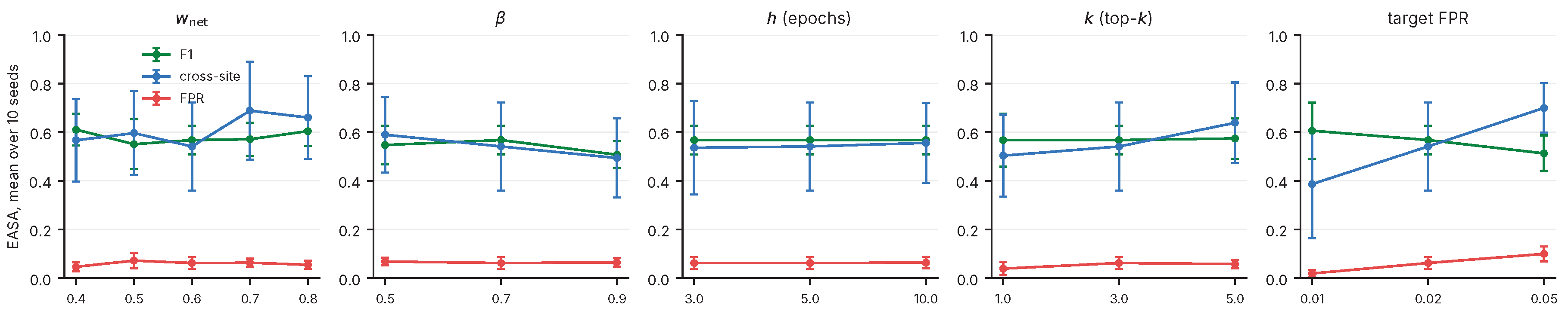
Table A2.
Sensitivity sweep: one parameter varied at a time around the defaults (10 seeds per point, in-process cloud mock).
Table A2.
Sensitivity sweep: one parameter varied at a time around the defaults (10 seeds per point, in-process cloud mock).
| Axis | Value | F1 | FPR | Cross-site | Contain. | Restricted share | Re-auth/dev-h | ||||||
|---|---|---|---|---|---|---|---|---|---|---|---|---|---|
| B3 net-only | EASA | B3 net-only | EASA | B3 net-only | EASA | B3 net-only | EASA | B3 net-only | EASA | B3 net-only | EASA | ||
| 0.4 | 0.535 | 0.611 | 0.063 | 0.047 | 0.591 | 0.567 | 0.772 | 0.821 | 0.150 | 0.186 | 0.258 | 0.214 | |
| 0.5 | 0.535 | 0.551 | 0.063 | 0.072 | 0.591 | 0.596 | 0.772 | 0.822 | 0.150 | 0.192 | 0.258 | 0.220 | |
| 0.6 | 0.535 | 0.568 | 0.063 | 0.062 | 0.591 | 0.541 | 0.772 | 0.834 | 0.150 | 0.177 | 0.258 | 0.257 | |
| 0.7 | 0.535 | 0.571 | 0.063 | 0.063 | 0.591 | 0.689 | 0.772 | 0.832 | 0.150 | 0.165 | 0.258 | 0.235 | |
| 0.8 | 0.535 | 0.604 | 0.063 | 0.055 | 0.591 | 0.660 | 0.772 | 0.846 | 0.150 | 0.160 | 0.258 | 0.238 | |
| 0.5 | 0.597 | 0.547 | 0.050 | 0.068 | 0.709 | 0.590 | 0.767 | 0.795 | 0.139 | 0.166 | 0.209 | 0.229 | |
| 0.7 | 0.535 | 0.568 | 0.063 | 0.062 | 0.591 | 0.541 | 0.772 | 0.834 | 0.150 | 0.177 | 0.258 | 0.257 | |
| 0.9 | 0.477 | 0.507 | 0.058 | 0.064 | 0.517 | 0.494 | 0.737 | 0.809 | 0.148 | 0.180 | 0.238 | 0.238 | |
| h (epochs) | 3 | 0.532 | 0.568 | 0.063 | 0.062 | 0.587 | 0.536 | 0.768 | 0.837 | 0.149 | 0.176 | 0.266 | 0.255 |
| 5 | 0.535 | 0.568 | 0.063 | 0.062 | 0.591 | 0.541 | 0.772 | 0.834 | 0.150 | 0.177 | 0.258 | 0.257 | |
| 10 | 0.529 | 0.568 | 0.064 | 0.064 | 0.587 | 0.556 | 0.772 | 0.838 | 0.153 | 0.180 | 0.252 | 0.257 | |
| k (top-k) | 1 | 0.531 | 0.567 | 0.029 | 0.039 | 0.429 | 0.503 | 0.606 | 0.717 | 0.094 | 0.135 | 0.277 | 0.238 |
| 3 | 0.535 | 0.568 | 0.063 | 0.062 | 0.591 | 0.541 | 0.772 | 0.834 | 0.150 | 0.177 | 0.258 | 0.257 | |
| 5 | 0.515 | 0.574 | 0.062 | 0.058 | 0.598 | 0.639 | 0.708 | 0.825 | 0.140 | 0.164 | 0.206 | 0.217 | |
| target FPR | 0.01 | 0.585 | 0.606 | 0.022 | 0.019 | 0.505 | 0.387 | 0.630 | 0.682 | 0.092 | 0.115 | 0.214 | 0.171 |
| 0.02 | 0.535 | 0.568 | 0.063 | 0.062 | 0.591 | 0.541 | 0.772 | 0.834 | 0.150 | 0.177 | 0.258 | 0.257 | |
| 0.05 | 0.516 | 0.513 | 0.078 | 0.100 | 0.659 | 0.700 | 0.811 | 0.903 | 0.162 | 0.206 | 0.366 | 0.305 | |
Three observations complement Section 5.10 (Table , Figure ; B3 has no fusion weights, so its rows repeat the default run; when varies the remainder is split between and in the default ratio). EASA’s calibrated tracks the fusion weight (0.71 at , 0.63 at the default, 0.54 at 0.8; B3 stays at 0.47): more weight on the noisier network term widens the benign trust distribution, so the threshold drops to hold the calibration-segment rate. The benign-side cost follows: the restricted share of benign epochs exceeds B3’s by 3.6 points at and 1.0 at 0.8, post-attack dwell by 417 and 141 s, so the lock-in of Section 5.7 is largest where the history term weighs most. Detection has no single direction: EASA’s F1 is higher at 15 of 17 points (exceptions , , and the 5% target, ), containment at every point, cross-site recall higher at six and lower at eleven (largest positive at , vs. ; largest negative at and the 1% target, each). The sweep varies one parameter at a time around a default at which the main experiment found no demonstrated detection value, so these points are exploratory; a fusion weight chosen on them would be chosen on the test traces.
Appendix D. Paired Differences
Table A2 and Table A3 give, per headline metric, the paired difference between EASA and each other configuration over the 30 seeds (same campaign schedule, phases and posture draws per seed): mean per-seed difference, 95% bootstrap confidence interval (2,000 seed resamples), two-sided paired Wilcoxon signed-rank p with Holm correction over the six comparisons per metric, and the number of seeds in which EASA is strictly better. Ties are excluded from the Wilcoxon statistic and the win count; metrics undefined in a seed are dropped pairwise. The per-seed result file is released with the code.
Table A3.
Paired differences versus EASA, detection metrics (Holm-corrected over six comparisons per metric).
Table A3.
Paired differences versus EASA, detection metrics (Holm-corrected over six comparisons per metric).
| Metric | vs. | (EASA − other) | 95% CI | p (Holm) | Seeds EASA better |
|---|---|---|---|---|---|
| F1 () | B0 static | +0.601 | 30/30 | ||
| B1 VNSF | +0.103 | 27/30 | |||
| B2 rules | +0.385 | 29/30 | |||
| B3 net-only | +0.037 | 0.090 | 21/30 | ||
| EASA−C | +0.162 | 26/30 | |||
| EASA−PH | −0.014 | 0.777 | 17/30 | ||
| FPR | B0 static | +0.054 | 0/30 | ||
| B1 VNSF | +0.001 | 1.000 | 14/30 | ||
| B2 rules | +0.007 | 1.000 | 9/30 | ||
| B3 net-only | +0.004 | 1.000 | 13/30 | ||
| EASA−C | +0.005 | 1.000 | 11/30 | ||
| EASA−PH | +0.004 | 1.000 | 13/30 | ||
| Recall (in-dist.) | B0 static | +0.756 | 30/30 | ||
| B1 VNSF | −0.065 | 0.088 | 9/30 | ||
| B2 rules | +0.612 | 29/30 | |||
| B3 net-only | −0.016 | 1.000 | 13/30 | ||
| EASA−C | +0.081 | 0.089 | 20/30 | ||
| EASA−PH | −0.016 | 1.000 | 13/30 | ||
| Recall (cross-site) | B0 static | +0.599 | 30/30 | ||
| B1 VNSF | +0.253 | 26/30 | |||
| B2 rules | +0.461 | 30/30 | |||
| B3 net-only | −0.028 | 0.980 | 13/30 | ||
| EASA−C | +0.362 | 29/30 | |||
| EASA−PH | −0.031 | 0.980 | 13/30 | ||
| Containment | B0 static | +0.849 | 30/30 | ||
| B1 VNSF | +0.167 | 23/30 | |||
| B2 rules | +0.584 | 29/30 | |||
| B3 net-only | +0.085 | 0.010 | 22/30 | ||
| EASA−C | +0.293 | 28/30 | |||
| EASA−PH | −0.000 | 0.666 | 14/30 | ||
| Replay catch (all runs) | B0 static | +0.806 | 29/30 | ||
| B1 VNSF | +0.624 | 28/30 | |||
| B2 rules | +0.642 | 26/30 | |||
| B3 net-only | +0.668 | 28/30 | |||
| EASA−C | +0.684 | 28/30 | |||
| EASA−PH | +0.049 | 0.355 | 10/30 |
Table A4.
Paired differences versus EASA, benign-side cost metrics (EASA is better when lower).
| Metric | vs. | (EASA − other) | 95% CI | p (Holm) | Seeds EASA better |
|---|---|---|---|---|---|
| False quarantine | B0 static | +0.042 | 0/30 | ||
| B1 VNSF | −0.034 | 21/30 | |||
| B2 rules | −0.035 | 0.002 | 19/30 | ||
| B3 net-only | +0.016 | 0.018 | 3/30 | ||
| EASA−C | +0.018 | 0.018 | 3/30 | ||
| EASA−PH | +0.016 | 0.018 | 3/30 | ||
| Re-auth / dev-h | B0 static | +0.228 | 0/30 | ||
| B1 VNSF | +0.228 | 0/30 | |||
| B2 rules | +0.228 | 0/30 | |||
| B3 net-only | −0.018 | 0.134 | 17/30 | ||
| EASA−C | +0.033 | 0.052 | 9/30 | ||
| EASA−PH | −0.018 | 0.134 | 16/30 | ||
| Restricted share (all benign epochs) | B0 static | +0.175 | 0/30 | ||
| B1 VNSF | +0.030 | 0.003 | 9/30 | ||
| B2 rules | +0.105 | 0/30 | |||
| B3 net-only | +0.035 | 5/30 | |||
| EASA−C | +0.055 | 4/30 | |||
| EASA−PH | +0.034 | 5/30 | |||
| Post-attack dwell (s) | B0 static | +1236 | 0/30 | ||
| B1 VNSF | +260 | 7/30 | |||
| B2 rules | +880 | 0/30 | |||
| B3 net-only | +285 | 5/30 | |||
| EASA−C | +454 | 3/30 | |||
| EASA−PH | +274 | 5/30 |
Appendix E. Sensitivity of the Labelling Rule
The dominant-source rule of Section 4.2 has three thresholds: the minimum flow share designating an address an attacker (5%), the attacker cap per ranking (8) and the weakness test excluding a type (attacker set below 40% of the capture and largest attacker below 25%). Over the full grid (27 settings) we recomputed the attacker sets and, per retained type, their Jaccard overlap with the default set and the share of rows relabelled (Table A4; scripts/label_sensitivity.py). The weakness threshold changes which low-coverage types are excluded, never an attacker set. A 3% share adds low-share addresses to the fragmented DDoS types and Mirai (Jaccard 0.57–0.77), relabelling up to 20% of one type’s rows and 0.4–1.9% of all retained rows; a cap of 6 truncates two of the four eight-attacker DDoS types (ACK fragmentation and HTTP flood, 13–15% of their rows); a 10% share removes attackers from most types (median Jaccard 0.50), relabelling 12% of all retained rows and 62% of the DDoS HTTP flood. The three high-volume DoS floods, which dominate the row count, are unaffected except by the 10% share on the SYN flood. Labels are thus stable under a tighter cap and a looser share, and sensitive to a stricter share, which would exclude attackers the default rule designates; whether those addresses are in fact attackers cannot be decided without the packet captures.
Table A5.
Sensitivity of the labelling rule to its thresholds on the raw captures: Jaccard overlap with the default attacker set and share of rows relabelled.
Table A5.
Sensitivity of the labelling rule to its thresholds on the raw captures: Jaccard overlap with the default attacker set and share of rows relabelled.
| min. share 3% | min. share 5% (default share) | min. share 10% | ||||||
|---|---|---|---|---|---|---|---|---|
| Attack type | Flows | Jaccard | rows changed (%) | Jaccard | rows changed (%) | Jaccard | rows changed (%) | |
| DDoS ACK fragmentation | 8 | 2,450,086 | 0.75 | 13.1 | 0.75 | 13.1 | 0.38 | 34.9 |
| DDoS ICMP flood | 8 | 202,251 | 0.57 | 10.6 | 0.88 | 0.3 | 0.25 | 13.6 |
| DDoS HTTP flood | 8 | 505,720 | 0.67 | 19.6 | 0.75 | 15.2 | 0.12 | 62.2 |
| DDoS ICMP fragmentation | 8 | 320,757 | 0.58 | 16.8 | 0.88 | 0.6 | 0.50 | 0.9 |
| DoS SYN flood | 4 | 16,290,644 | 0.67 | 0.0 | 1.00 | 0.0 | 0.50 | 11.7 |
| DoS HTTP flood | 1 | 1,642,744 | 1.00 | 0.0 | 1.00 | 0.0 | 1.00 | 0.0 |
| DoS UDP flood | 2 | 5,210,536 | 0.67 | 0.0 | 1.00 | 0.0 | 1.00 | 0.0 |
| Mirai | 11 | 174,588 | 0.77 | 11.4 | 0.91 | 0.2 | 0.64 | 23.2 |
| Vulnerability scan | 3 | 442,158 | 0.75 | 4.0 | 1.00 | 0.0 | 0.67 | 6.7 |
| DNS spoofing | 5 | 74,856 | 0.83 | 4.8 | 1.00 | 0.0 | 0.40 | 21.7 |
| SQL injection | 3 | 6,603 | 0.60 | 8.7 | 1.00 | 0.0 | 0.33 | 14.9 |
The shares above are computed on the raw captures, where the three high-volume DoS floods hold 85% of the retained rows; on the family-balanced working data of Table 6 the same alternative attacker sets move more of the rows the experiments use (Table A5): a 3% minimum share relabels 3.1% of working rows (3.4% of training rows; up to 16% of one DDoS type and 11% of Mirai), a cap of 6 relabels 2.7%, a cap of 12 relabels 0.4%, and a 10% minimum share relabels 17.6% (16.9% of training rows, 18.4% of test rows; 76% of the DDoS HTTP flood). Two distinctions matter. First, the benign device traces driving calibration and false-positive evaluation come from the benign capture chain only and are unaffected by every setting; the rule moves only the detector’s training labels and the attack-labelled capture records. Second, in the replayed designated-attacker traces a campaign emits, adding attackers (3%, or a cap of 12) removes no attack label, a cap of 6 removes it from 2.5% of trace records (7.8% of the DDoS traces), and the 10% share from 24.8% (45% of the DDoS, 50% of the Mirai, 51% of the Spoofing and 21% of the Web trace records; the DDoS ICMP and HTTP flood traces lose 100% and 95%). A detector trained under the 10% rule would therefore see substantially different positives and a campaign from the same traces substantially fewer attack-labelled records; we did not retrain or re-evaluate under any alternative rule, so the main comparisons are conditional on the default rule, and the per-family results show where that dependence is largest (DDoS, Mirai, Spoofing, Web).
Table A6.
Sensitivity of the labelling rule on the working data and the replayed attacker traces.
| 3%, 8 | 5%, 6 | 5%, 12 | 10%, 8 | |||||||
|---|---|---|---|---|---|---|---|---|---|---|
| Attack type | Rows | Trace rec. | rows % | traces % | rows % | traces % | rows % | traces % | rows % | traces % |
| DDoS ACK fragmentation | 352,116 | 92,959 | 0.0 | 0.0 | 9.6 | 10.1 | 0.0 | 0.0 | 32.5 | 35.9 |
| DDoS ICMP flood | 31,708 | 975 | 10.3 | 0.0 | 0.3 | 0.0 | 0.0 | 0.0 | 13.0 | 100.0 |
| DDoS HTTP flood | 72,684 | 21,289 | 0.0 | 0.0 | 16.3 | 0.0 | 8.6 | 0.0 | 76.3 | 94.8 |
| DDoS ICMP fragmentation | 46,060 | 5,064 | 16.3 | 0.0 | 0.6 | 1.1 | 0.0 | 0.0 | 0.8 | 1.1 |
| DoS SYN flood | 351,924 | 104,426 | 0.0 | 0.0 | 0.0 | 0.0 | 0.0 | 0.0 | 10.5 | 11.1 |
| DoS HTTP flood | 35,484 | 8,653 | 0.0 | 0.0 | 0.0 | 0.0 | 0.0 | 0.0 | 0.0 | 0.0 |
| DoS UDP flood | 112,784 | 30,351 | 0.0 | 0.0 | 0.0 | 0.0 | 0.0 | 0.0 | 0.0 | 0.0 |
| Mirai | 174,588 | 24,470 | 11.4 | 0.0 | 0.2 | 0.4 | 0.0 | 0.0 | 23.2 | 50.2 |
| Vulnerability scan | 442,158 | 79,719 | 4.0 | 0.0 | 0.0 | 0.0 | 0.0 | 0.0 | 6.7 | 13.2 |
| DNS spoofing | 74,856 | 9,401 | 4.8 | 0.0 | 0.0 | 0.0 | 0.0 | 0.0 | 21.7 | 50.9 |
| SQL injection | 6,603 | 1,304 | 8.7 | 0.0 | 0.0 | 0.0 | 0.0 | 0.0 | 14.9 | 21.4 |
| All retained types | 1,700,965 | 378,611 | 3.1 | 0.0 | 2.7 | 2.5 | 0.4 | 0.0 | 17.6 | 24.8 |
Appendix F. Implementation Audit of the Replay Protocol
The replay invariants of Section 4.3 and Section 4.5 were checked on the working pool with the released script scripts/audit_protocol.py; its output is reproduced below. It checks availability-time order (start plus duration, capped at the 120 s flow timeout) in every replay trace and counts the records moved relative to start order; reports the maximum recorded duration, distinguishing records exactly at the cap from those strictly above it (only the latter would become visible before their real end) and whether any occur in replay traces; checks that no device’s calibration and evaluation segments share a record or overlap in time and counts records that start in one and become available in the other; reports how often a trace wraps within a one-hour run and that every virtual clock is monotone; and lists the evaluation sample (records per segment and per designated attacker trace, and the test split’s absolute time range).
Table A7.
Implementation audit of the replay protocol on the working pool.
| Invariant | Check | Result |
|---|---|---|
| Duration cap | raw Flow Duration in s (unclipped), vs. the 120 s cap | maximum recorded duration 120.000 s; 0 rows above the cap; 40 rows exactly at it (train 22, val 3, test 15; 0.002%), of which 3 occur in calibration traces, 6 in evaluation traces and 1 in an attacker trace; 1,085 zero-duration rows (0.05%) visible at start |
| Availability order | every trace sorted by start + duration | OK for all traces; 362,285 of 497,014 trace records (72.9%) change position relative to start order |
| Segment boundary | calibration vs. evaluation segment per device | 65 devices; 39,425 calibration and 78,978 evaluation records; 0 shared; 0 devices with overlapping time ranges; 95 straddling records assigned to evaluation |
| Wrap | trace duration vs. run / pass / campaign length | evaluation traces: median 16,027 s, min 188 s, 7 of 65 shorter than one run; calibration traces: median 7,512 s, min 60 s, 8 of 65 shorter than the pass; attacker traces shorter than 600 s: DoS 2 of 5, Web 3 of 3 (DDoS, Mirai, Recon, Spoofing: none) |
| Virtual clock | cumulative clipped gaps | monotone in every trace |
| Sample | records per designated-attacker trace; test-split time range | test split 629,875 rows, 2022-08-02 12:00 to 2023-01-18 11:52; DDoS 13 traces (58–21,183), DoS 5 (81–73,719), Mirai 11 (90–11,058), Recon 3 (835–68,391), Spoofing 5 (894–2,829), Web 3 (131–1,025) |
Table A6 summarises the output; four findings qualify the protocol statements of Section 4 and are carried into the limitations. (i) No recorded duration exceeds 120 s (maximum exactly 120.000 s), because CICFlowMeter terminates a flow at its own 120 s timeout, so the cap of the availability rule is never binding and no record is made visible before the extractor would have emitted it; 40 rows (0.002%; 15 in the test split) sit exactly at the timeout (3 in calibration, 6 in evaluation and 1 in attacker traces, all replayed at the correct time), and 1,085 zero-duration single-packet rows (0.05%) are visible at their start, as an online extractor would report them. (ii) The availability rule is not cosmetic: 72.9% of replay-trace records change position relative to start order. (iii) The 65 devices’ calibration and evaluation segments share no record and do not overlap in time; 95 evaluation records (0.1%) that started before the calibration segment ended and became available after it are assigned to evaluation. (iv) Traces wrap: 7 of the 65 evaluation traces are shorter than the 3,600 s run (the shortest, 188 s, is replayed about 19 times), 8 calibration traces than the 1,800 s pass, and 2 of the 5 DoS and all 3 Web designated-attacker traces than the longest campaign (600 s), so those families can replay the same burst more than once. Every virtual clock is monotone, and all records are CICFlowMeter flow records as released, without further aggregation.
References
- Roman, R.; Lopez, J.; Mambo, M. Mobile Edge Computing, Fog et al.: A Survey and Analysis of Security Threats and Challenges. Future Gener. Comput. Syst. 2018, 78, 680–698. [Google Scholar] [CrossRef]
- Xiao, Y.; Jia, Y.; Liu, C.; Cheng, X.; Yu, J.; Lv, W. Edge Computing Security: State of the Art and Challenges. Proc. IEEE 2019, 107, 1608–1631. [Google Scholar] [CrossRef]
- Bittencourt, L.; Immich, R.; Sakellariou, R.; Fonseca, N.; Madeira, E.; Curado, M.; Villas, L.; DaSilva, L.; Lee, C.; Rana, O. The Internet of Things, Fog and Cloud Continuum: Integration and Challenges. Internet Things 2018, 3–4, 134–155. [Google Scholar] [CrossRef]
- Google Threat Intelligence Group. GTIG AI Threat Tracker: From Prompting to Autonomy—The Evolution of Adversarial AI. 2026. Available online: https://cloud.google.com/blog/topics/threat-intelligence/from-prompting-to-autonomy-the-evolution-of-adversarial-ai (accessed on 10 October 2026).
- Anthropic. Detecting and Countering Misuse of AI: September 2026. Available online: https://www.anthropic.com/threat-intelligence-report-september-2026 (accessed on 10 October 2026).
- Canavese, D.; Mannella, L.; Regano, L.; Basile, C. Security at the Edge for Resource-Limited IoT Devices. Sensors 2024, 24, 590. [Google Scholar] [CrossRef]
- Rivera-Julio, Y.E.; Leal-Narváez, E.A.; Tejedor, J.P. Blockchain-Backed Revocation and Yang–Baxter Consistency Screening for Zero-Trust IoT Admission Control. Sensors 2026, 26, 5960. [Google Scholar] [CrossRef]
- Alanazi, A.G.; Alanazi, H.A. EdgeGuard-AI: Zero-Trust and Load-Aware Federated Scheduling for Secure and Low-Latency IoT Edge Networks. Sensors 2026, 26, 1989. [Google Scholar] [CrossRef]
- Ashfaq, F.; Wasim, M.; Shah, M.A.; Ahad, A.; Pires, I.M. Enhancing Security in 5G Edge Networks: Predicting Real-Time Zero Trust Attacks Using Machine Learning in SDN Environments. Sensors 2025, 25, 1905. [Google Scholar] [CrossRef]
- Rose, S.; Borchert, O.; Mitchell, S.; Connelly, S. 2020. Zero Trust Architecture. Technical Report NIST Special Publication 800-207. National Institute of Standards and Technology. [Google Scholar] [CrossRef]
- Syed, N.F.; Shah, S.W.; Shaghaghi, A.; Anwar, A.; Baig, Z.; Doss, R. Zero Trust Architecture (ZTA): A Comprehensive Survey. IEEE Access 2022, 10, 57143–57179. [Google Scholar] [CrossRef]
- Rabbani, M.; Gui, J.; Nejati, F.; Zhou, Z.; Kaniyamattam, A.; Mirani, M.; Piya, G.; Opushnyev, I.; Lu, R.; Ghorbani, A.A. Device Identification and Anomaly Detection in IoT Environments. IEEE Internet Things J. 2025, 12, 13625–13643. [Google Scholar] [CrossRef]
- Canadian Institute for Cybersecurity. CIC IoT-DIAD 2024: IoT Device Identification and Anomaly Detection Dataset. 2024. Available online: https://www.unb.ca/cic/datasets/iot-diad-2024.html (accessed on 10 October 2026).
- Wu, T.Y.; Meng, Q.; Kumari, S.; Zhang, P. Rotating behind Security: A Lightweight Authentication Protocol Based on IoT-Enabled Cloud Computing Environments. Sensors 2022, 22, 3858. [Google Scholar] [CrossRef]
- Ju, S.; Park, Y. Provably Secure Lightweight Mutual Authentication and Key Agreement Scheme for Cloud-Based IoT Environments. Sensors 2023, 23, 9766. [Google Scholar] [CrossRef]
- Li, M.; Hu, S. A Lightweight ECC-Based Authentication and Key Agreement Protocol for IoT with Dynamic Authentication Credentials. Sensors 2024, 24, 7967. [Google Scholar] [CrossRef]
- Raza, S.; Shafagh, H.; Hewage, K.; Hummen, R.; Voigt, T. Lithe: Lightweight Secure CoAP for the Internet of Things. IEEE Sens. J. 2013, 13, 3711–3720. [Google Scholar] [CrossRef]
- Miettinen, M.; Marchal, S.; Hafeez, I.; Asokan, N.; Sadeghi, A.R.; Tarkoma, S. IoT SENTINEL: Automated Device-Type Identification for Security Enforcement in IoT. In Proceedings of the 37th IEEE International Conference on Distributed Computing Systems (ICDCS), Atlanta, GA, USA, June 2017; pp. 2177–2184. [Google Scholar] [CrossRef]
- Hafeez, I.; Antikainen, M.; Ding, A.Y.; Tarkoma, S. IoT-KEEPER: Detecting Malicious IoT Network Activity Using Online Traffic Analysis at the Edge. IEEE Trans. Netw. Serv. Manag. 2020, 17, 45–59. [Google Scholar] [CrossRef]
- Nguyen, X.H.; Nguyen, X.D.; Huynh, H.H.; Le, K.H. Realguard: A Lightweight Network Intrusion Detection System for IoT Gateways. Sensors 2022, 22, 432. [Google Scholar] [CrossRef]
- Subramanian, C.; Santhanam, B. Adaptive Internet of Things Edge Device Security. Intel Corporation: Assignee, April 2020. Available online: https://patents.google.com/patent/US10616249B2/en.
- Buck, C.; Olenberger, C.; Schweizer, A.; Völter, F.; Eymann, T. Never Trust, Always Verify: A Multivocal Literature Review on Current Knowledge and Research Gaps of Zero-Trust. Comput. Secur. 2021, 110, 102436. [Google Scholar] [CrossRef]
- Mthethwa, S.; Dlamini, M.T.; Jembere, E. Zero Trust for NHIs Based on Robust Identity and Access Management for a Resilient IoT Future. Sensors 2026, 26, 2392. [Google Scholar] [CrossRef]
- Ometov, A.; Molua, O.L.; Komarov, M.; Nurmi, J. A Survey of Security in Cloud, Edge, and Fog Computing. Sensors 2022, 22, 927. [Google Scholar] [CrossRef]
- Yan, Z.; Zhang, P.; Vasilakos, A.V. A Survey on Trust Management for Internet of Things. J. Netw. Comput. Appl. 2014, 42, 120–134. [Google Scholar] [CrossRef]
- Chen, I.R.; Bao, F.; Guo, J. Trust-Based Service Management for Social Internet of Things Systems. IEEE Trans. Dependable Secur. Comput. 2016, 13, 684–696. [Google Scholar] [CrossRef]
- Liu, Y.; Wang, J.; Yan, Z.; Wan, Z.; Jäntti, R. A Survey on Blockchain-Based Trust Management for Internet of Things. IEEE Internet Things J. 2023, 10, 5898–5922. [Google Scholar] [CrossRef]
- Dimitrakos, T.; Dilshener, T.; Kravtsov, A.; La Marra, A.; Martinelli, F.; Rizos, A.; Rosetti, A.; Saracino, A. Trust Aware Continuous Authorization for Zero Trust in Consumer Internet of Things. In Proceedings of the 19th IEEE International Conference on Trust, Security and Privacy in Computing and Communications (TrustCom), Guangzhou, China, December 2020; pp. 1801–1812. [Google Scholar] [CrossRef]
- Jeong, E.; Yang, D. A Trust Score-Based Access Control Model for Zero Trust Architecture: Design, Sensitivity Analysis, and Real-World Performance Evaluation. Appl. Sci. 2025, 15, 9551. [Google Scholar] [CrossRef]
- Aydin, H. A Federated Multi-Agent Communication Framework for Autonomous Cyber Defense in Edge–Cloud IoT Environments. Sensors 2026, 26, 5775. [Google Scholar] [CrossRef]
- McMahan, B.; Moore, E.; Ramage, D.; Hampson, S.; Agüera y Arcas, B. Communication-Efficient Learning of Deep Networks from Decentralized Data. In Proceedings of the 20th International Conference on Artificial Intelligence and Statistics (AISTATS), Fort Lauderdale, FL, USA, April 2017; Vol. 54, PMLR, pp. 1273–1282. Available online: https://proceedings.mlr.press/v54/mcmahan17a.html.
- Li, T.; Sahu, A.K.; Talwalkar, A.; Smith, V. Federated Learning: Challenges, Methods, and Future Directions. IEEE Signal Process. Mag. 2020, 37, 50–60. [Google Scholar] [CrossRef]
- Rahman, S.A.; Tout, H.; Talhi, C.; Mourad, A. Internet of Things Intrusion Detection: Centralized, On-Device, or Federated Learning? IEEE Netw. 2020, 34, 310–317. [Google Scholar] [CrossRef]
- Mothukuri, V.; Khare, P.; Parizi, R.M.; Pouriyeh, S.; Dehghantanha, A.; Srivastava, G. Federated-Learning-Based Anomaly Detection for IoT Security Attacks. IEEE Internet Things J. 2022, 9, 2545–2554. [Google Scholar] [CrossRef]
- Nguyen, T.D.; Marchal, S.; Miettinen, M.; Fereidooni, H.; Asokan, N.; Sadeghi, A.R. DÏoT: A Federated Self-learning Anomaly Detection System for IoT. In Proceedings of the 39th IEEE International Conference on Distributed Computing Systems (ICDCS), Dallas, TX, USA, July 2019; pp. 756–767. [Google Scholar] [CrossRef]
- Nguyen, T.D.; Rieger, P.; Miettinen, M.; Sadeghi, A.R. Poisoning Attacks on Federated Learning-Based IoT Intrusion Detection System. In Proceedings of the Workshop on Decentralized IoT Systems and Security (DISS), co-located with NDSS, San Diego, CA, USA, February 2020. [Google Scholar] [CrossRef]
- Ferrag, M.A.; Friha, O.; Hamouda, D.; Maglaras, L.; Janicke, H. Edge-IIoTset: A New Comprehensive Realistic Cyber Security Dataset of IoT and IIoT Applications for Centralized and Federated Learning. IEEE Access 2022, 10, 40281–40306. [Google Scholar] [CrossRef]
- Sommer, R.; Paxson, V. Outside the Closed World: On Using Machine Learning for Network Intrusion Detection. In Proceedings of the 2010 IEEE Symposium on Security and Privacy, Oakland, CA, USA, May 2010; pp. 305–316. [Google Scholar] [CrossRef]
- Ring, M.; Wunderlich, S.; Scheuring, D.; Landes, D.; Hotho, A. A Survey of Network-Based Intrusion Detection Data Sets. Comput. Secur. 2019, 86, 147–167. [Google Scholar] [CrossRef]
- Sivanathan, A.; Gharakheili, H.H.; Loi, F.; Radford, A.; Wijenayake, C.; Vishwanath, A.; Sivaraman, V. Classifying IoT Devices in Smart Environments Using Network Traffic Characteristics. IEEE Trans. Mob. Comput. 2019, 18, 1745–1759. [Google Scholar] [CrossRef]
- Kolias, C.; Kambourakis, G.; Stavrou, A.; Voas, J. DDoS in the IoT: Mirai and Other Botnets. Computer 2017, 50, 80–84. [Google Scholar] [CrossRef]
- Neto, E.C.P.; Dadkhah, S.; Ferreira, R.; Zohourian, A.; Lu, R.; Ghorbani, A.A. CICIoT2023: A Real-Time Dataset and Benchmark for Large-Scale Attacks in IoT Environment. Sensors 2023, 23, 5941. [Google Scholar] [CrossRef]
- Moustafa, N. A New Distributed Architecture for Evaluating AI-Based Security Systems at the Edge: Network TON_IoT Datasets. Sustain. Cities Soc. 2021, 72, 102994. [Google Scholar] [CrossRef]
- Purkaystha, C.; Gandhi, Y.N.; Kumar, P. Uncertainty-Aware Zero-Day Botnet Detection for IoT Networks with Real-World Edge Deployment on Resource-Constrained Hardware. Sensors 2026, 26, 5863. [Google Scholar] [CrossRef]
- Choobdar, P.; Davies, N.; Wilson, E.D.; Hodges, S.; Jude, E.B.; Bradbury, M.; Reeves, N.D. Cybersecurity of Smart Sensing Insole Systems: A Threat Modelling Approach to Understanding Security Vulnerabilities. Sensors 2026, 26, 6298. [Google Scholar] [CrossRef]
- Lashkari, A.H.; Draper-Gil, G.; Mamun, M.S.I.; Ghorbani, A.A. Characterization of Tor Traffic Using Time Based Features. In Proceedings of the 3rd International Conference on Information Systems Security and Privacy (ICISSP), Porto, Portugal, February 2017; pp. 253–262. [Google Scholar] [CrossRef]
- Blanchard, P.; El Mhamdi, E.M.; Guerraoui, R.; Stainer, J. Machine Learning with Adversaries: Byzantine Tolerant Gradient Descent. In Proceedings of the 31st Conference on Neural Information Processing Systems (NeurIPS 2017), Long Beach, CA, USA, December 2017; pp. 119–129. Available online: https://proceedings.neurips.cc/paper/2017/hash/f4b9ec30ad9f68f89b29639786cb62ef-Abstract.html.
- Yin, D.; Chen, Y.; Ramchandran, K.; Bartlett, P. Byzantine-Robust Distributed Learning: Towards Optimal Statistical Rates. In Proceedings of the 35th International Conference on Machine Learning (ICML), Stockholm, Sweden, July 2018; Vol. 80, PMLR, pp. 5650–5659. Available online: https://proceedings.mlr.press/v80/yin18a.html.
- Firouzi, A.; Dadkhah, S.; Maret, S.A.; Ghorbani, A.A. DataSense: A Real-Time Sensor-Based Benchmark Dataset for Attack Analysis in IIoT with Multi-Objective Feature Selection. Electronics 2025, 14, 4095. [Google Scholar] [CrossRef]
Figure 2.
Six headline metrics over 30 seeds (box: interquartile range; line: median; whiskers: 1.5 IQR; dots: outliers; dashed line: 2% calibration target; EASA hatched).
Figure 2.
Six headline metrics over 30 seeds (box: interquartile range; line: median; whiskers: 1.5 IQR; dots: outliers; dashed line: 2% calibration target; EASA hatched).
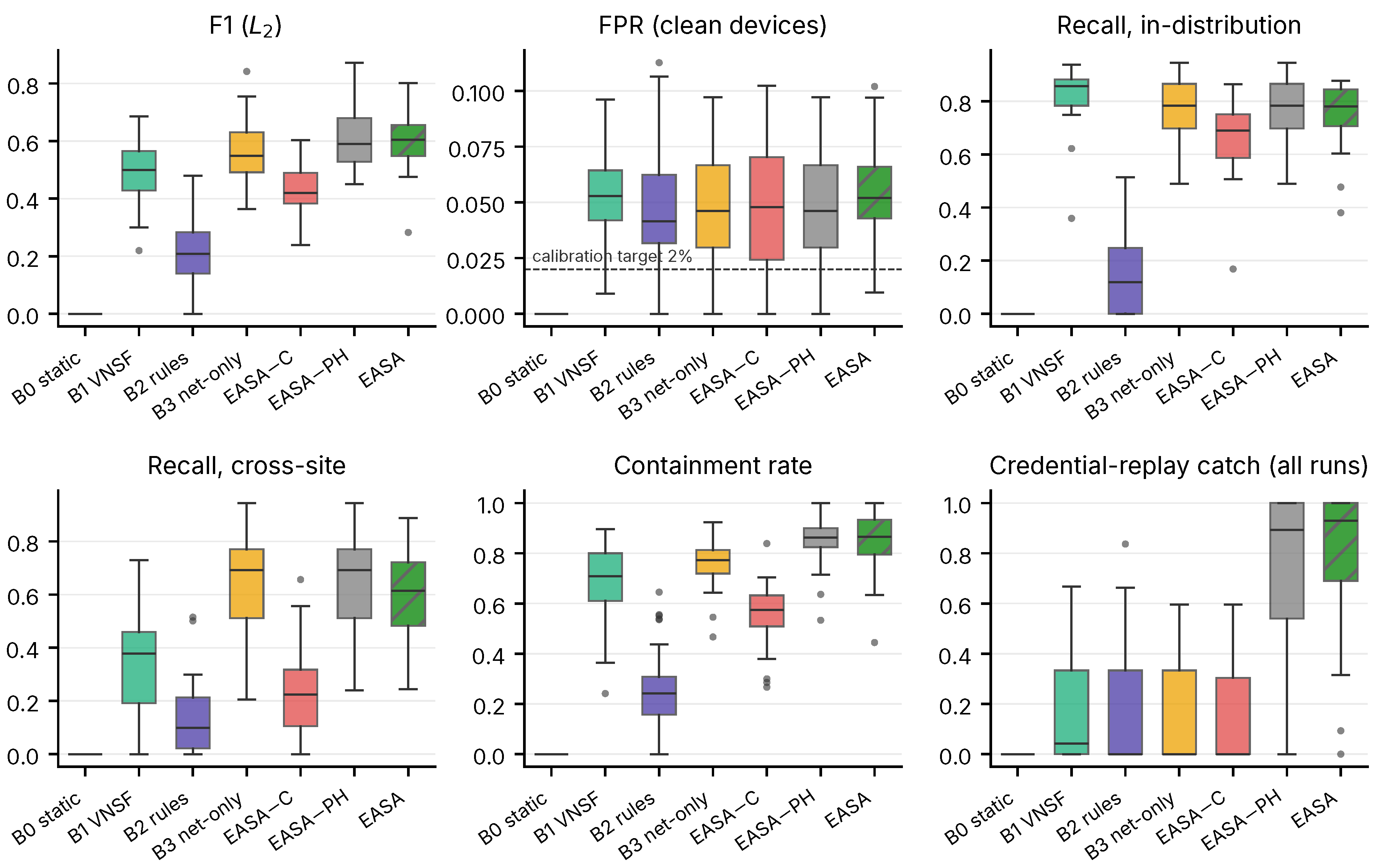
Figure 3.
Mean recall at the boundary over the runs in which each family occurs (run counts in Table 11; B0 and FirmwareTamper omitted).
Figure 3.
Mean recall at the boundary over the runs in which each family occurs (run counts in Table 11; B0 and FirmwareTamper omitted).
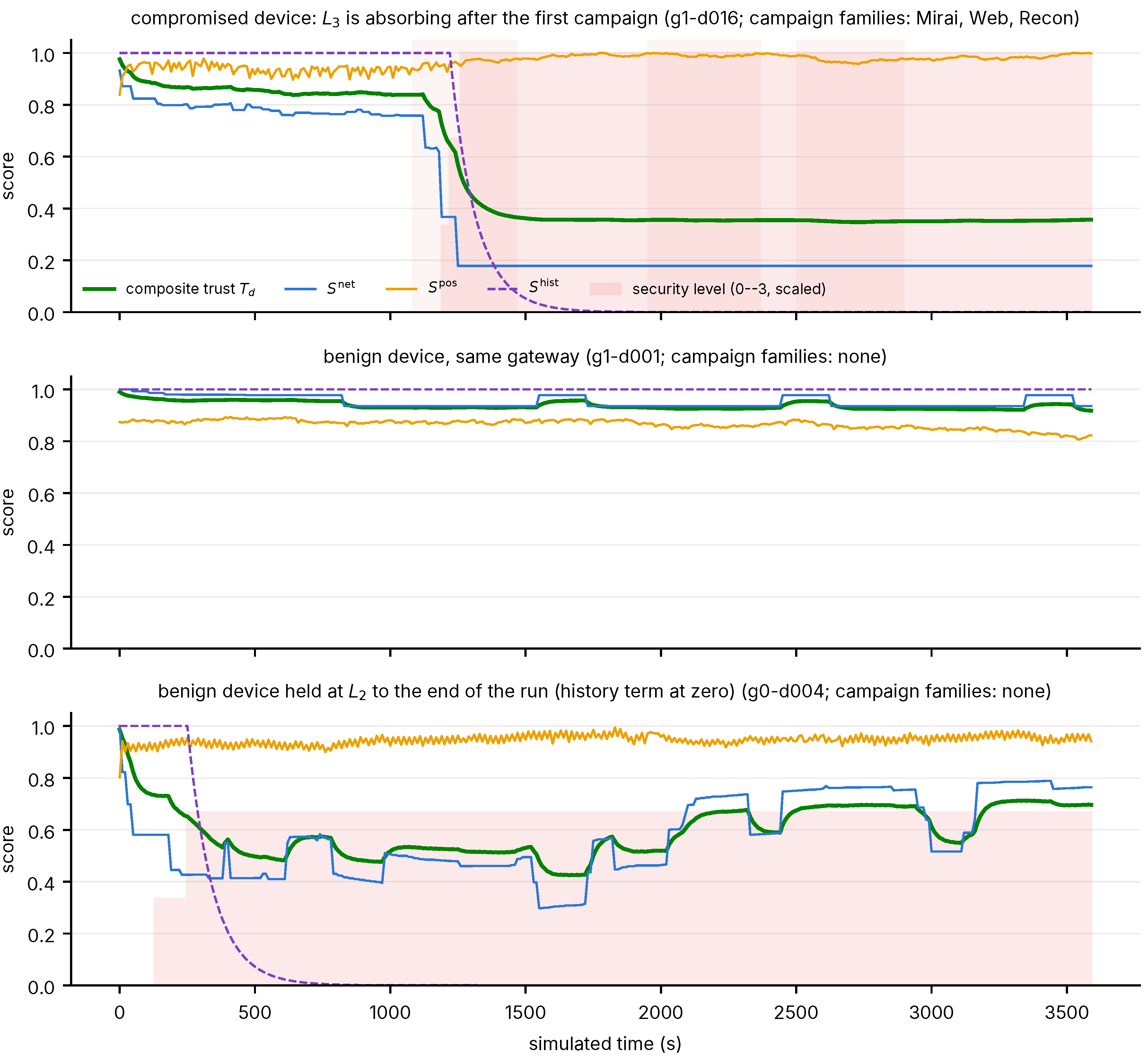
Figure 4.
Mean in-distribution and locally held-out-family (cross-site) recall at by configuration (30 seeds).
Figure 4.
Mean in-distribution and locally held-out-family (cross-site) recall at by configuration (30 seeds).
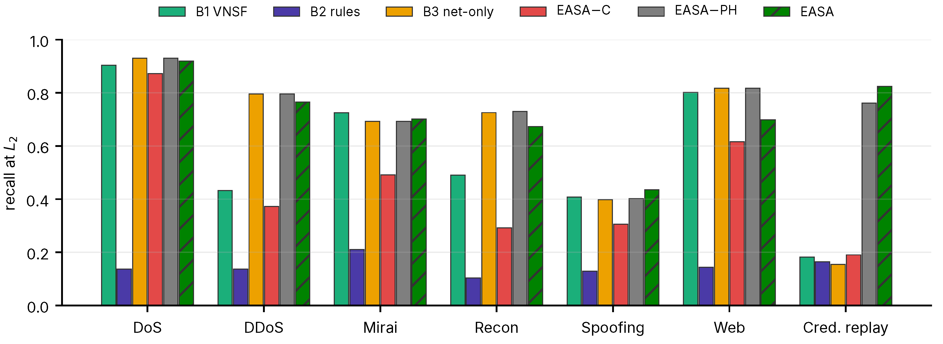
Figure 5.
EASA with the cloud reachable and during a 900 s outage after warm-up (30 paired seeds; box: interquartile range; line: median; whiskers: 1.5 IQR): replay rejection decreases, with no change detected in the evaluated local metrics.
Figure 5.
EASA with the cloud reachable and during a 900 s outage after warm-up (30 paired seeds; box: interquartile range; line: median; whiskers: 1.5 IQR): replay rejection decreases, with no change detected in the evaluated local metrics.
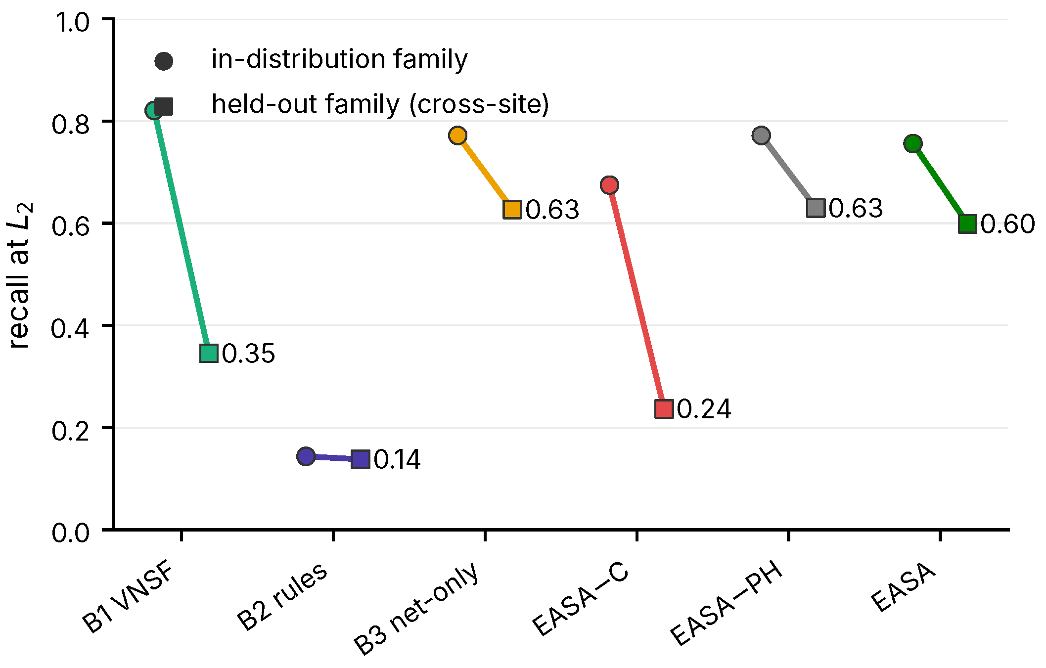
Table 3.
Transition rules of the PDP, one row per case.
| Condition | New level | Action and state |
|---|---|---|
| or credential revoked | drop traffic; publish revocation if ; persists while the condition holds | |
| for some | highest such | immediate; clean-epoch counter reset; on entering : re-handshake, or pending if |
| for h consecutive epochs | one level per h epochs; pending step-up cancelled if new level | |
| otherwise | ℓ | none; if and a step-up is pending and : execute re-handshake, clear pending |
Table 4.
EASA API primitives and their implementation status.
| Primitive | Caller→Callee | Freq. | Purpose | Status |
|---|---|---|---|---|
| POST /posture | D→E | per epoch | Posture beacon , signed. | emu |
| GET /trust/{d} | D→E | on demand | Current level and required action (e.g. re-auth). | emu |
| POST /auth/stepup | D→E | on | Challenge–response or mTLS re-handshake endpoint. | emu |
| POST /policy/evaluate | E (internal) | per epoch | TSE→PDP: returns given , posture, hysteresis state. | emu |
| POST /policy/enforce | E (internal) | on change | PDP→PEP: applies Table 2 actions. | emu |
| POST /sync/stats | E→C | hourly | Push local parameters (and sample count) for aggregation. | net |
| GET /sync/model | E→C | hourly | Pull aggregated with its version. | net |
| POST /revocations | E→C | on | Publish a revoked credential. | net |
| GET /sync/revocations | E→C | 5 min | Pull revoked credentials from all gateways. | net |
| POST /audit | E→C | on event | Level transitions, enforcement actions, model version. | net |
| GET /sync/policy | E→C | hourly | Pull versioned per device class. | spec |
Table 5.
Baselines and ablations expressed as EASA configurations.
| Configuration | Trust input | Enforcement | Cloud sync | Inspired by |
|---|---|---|---|---|
| B0 static | none (fixed auth) | none | none | lightweight AKA [14,15,16] |
| B1 VNSF | IPS alarm only | block/allow | none | IoT Proxy [6] |
| B2 rules | freshness/context rules | admit/reject | revocation only | YB-IoT-CG [7] |
| B3 net-only | only | 4 levels, always re-handshake | model only | EdgeGuard-AI [8] |
| EASA−C | composite | 4 levels, energy-aware | none | ablation: cloud removed |
| EASA−PH | only | 4 levels, energy-aware | model + revocation + audit | ablation: posture and history removed |
| EASA | composite | 4 levels, energy-aware | model + revocation + audit | proposed |
Table 6.
Working dataset after labelling, sampling and splitting.
| Family | Rows | Replayable attacker traces† | Attack types retained |
|---|---|---|---|
| Benign | 811,837 | – | benign chain + background traffic of attack captures |
| DDoS | 394,039 | 13 | ACK fragmentation, ICMP flood, HTTP flood, ICMP fragmentation |
| DoS | 482,715 | 5 | SYN flood, UDP flood, HTTP flood (TCP flood files corrupt, excluded) |
| Mirai | 80,683 | 11 | Mirai GRE/UDP floods |
| Recon | 288,623 | 3 | Vulnerability scan |
| Spoofing | 37,360 | 5 | DNS spoofing (ARP spoofing excluded) |
| Web | 4,038 | 3 | SQL injection (upload and XSS excluded) |
| Total 2,099,295 rows, 77 features; train / val / test = 1,259,535 / 209,885 / 629,875 rows (training 1,148,306 after de-duplication). † Designated attackers (Appendix A) whose flows occur in the test split of their capture and can therefore be replayed. | |||
Table 7.
Emulation and policy parameters.
| Parameter | Value | Note |
|---|---|---|
| Gateways / devices | 3 / 65 (22, 22, 21) | real device addresses with a benign trace |
| Decision epoch / flow window | 10 s / 120 s | window = CICFlowMeter default flow timeout |
| Run length / seeds | 3,600 s / 30 | mean ± std and 95% bootstrap CI |
| Campaigns per run | 10 | 3 forced cross-site, 1 forced credential replay, 6 sampled |
| Onset / duration | s / s | |
| Compromised fraction | 15% of a gateway’s devices | per campaign |
| Replay / tamper probability | 0.10 / 0.10 | among sampled campaigns |
| Held-out family | : DDoS, : Recon, : Spoofing | absent from that gateway’s training split |
| Device classes (share) | camera 0.25, hub 0.15, sensor 0.40, appliance 0.20 | |
| Battery (Wh) / idle (W) / per flow (mWh) | 20/1.2/0.6; 40/2.0/0.3; 5/0.05/0.15; mains | camera; hub; sensor; appliance |
| Re-authentication cost | 8 mWh | energy floor |
| 0.60, 0.25, 0.15 | Eq. 4 | |
| / | 0.70 / 0.90 | Eqs. 4, 3 |
| 0.40, 0.30, 0.30 | Eq. 2 | |
| Window score | top-k mean, , zero-padded | Section 4.5 |
| Flow availability | start + duration ( s) | a record is visible when an online extractor could emit it |
| Calibration segment | first 1/3 of each device’s test records (availability order) | benign pass only; the run replays the remaining 2/3 |
| Thresholds | calibrated per run | benign pass on the calibration segment, target FPR 2% |
| Hysteresis h / | 5 epochs (50 s) / | |
| L2 rate limit / L3 release | 2 flows/s / 600 s | release applies to reinstated credentials only; not exercised (every entry revokes) |
| Model sync / revocation poll | 300 s / 30 s | simulated time; design defaults 1 h / 5 min (Table 4) |
Table 8.
Main results over 30 seeds (mean ± sample std).
| Configuration | F1 () | FPR | Recall (in-dist.) | Recall (cross-site) | Containment | TTC p50 (s) | False quarantine | Re-auth / dev-h | Replay catch (all runs) |
|---|---|---|---|---|---|---|---|---|---|
| B0 static | 0.000 ± 0.000 | 0.000 ± 0.000 | 0.000 ± 0.000 | 0.000 ± 0.000 | 0.000 ± 0.000 | – | 0.000 ± 0.000 | 0.000 ± 0.000 | 0.000 ± 0.000 |
| B1 VNSF | 0.497 ± 0.106 | 0.053 ± 0.023 | 0.821 ± 0.110 | 0.346 ± 0.178 | 0.681 ± 0.148 | 42 ± 19 | 0.077 ± 0.032 | 0.000 ± 0.000 | 0.182 ± 0.229 |
| B2 rules | 0.216 ± 0.123 | 0.047 ± 0.029 | 0.144 ± 0.138 | 0.138 ± 0.138 | 0.265 ± 0.164 | 61 ± 79 | 0.077 ± 0.042 | 0.000 ± 0.000 | 0.165 ± 0.256 |
| B3 net-only | 0.564 ± 0.108 | 0.050 ± 0.024 | 0.772 ± 0.114 | 0.627 ± 0.217 | 0.763 ± 0.095 | 35 ± 17 | 0.026 ± 0.017 | 0.247 ± 0.057 | 0.138 ± 0.170 |
| EASA−C | 0.439 ± 0.089 | 0.048 ± 0.027 | 0.675 ± 0.142 | 0.237 ± 0.165 | 0.555 ± 0.134 | 58 ± 34 | 0.024 ± 0.019 | 0.195 ± 0.065 | 0.122 ± 0.168 |
| EASA−PH | 0.615 ± 0.102 | 0.050 ± 0.024 | 0.772 ± 0.114 | 0.630 ± 0.214 | 0.849 ± 0.099 | 33 ± 20 | 0.026 ± 0.017 | 0.246 ± 0.057 | 0.757 ± 0.295 |
| EASA | 0.601 ± 0.098 | 0.054 ± 0.023 | 0.756 ± 0.117 | 0.599 ± 0.172 | 0.849 ± 0.127 | 38 ± 24 | 0.042 ± 0.029 | 0.228 ± 0.047 | 0.806 ± 0.283 |
Table 9.
Benign-side cost over 30 seeds (mean ± std).
| Configuration | FPR (clean devices) | Restricted share (all benign epochs) | Post-attack dwell (s / compromised device) | False quarantine |
|---|---|---|---|---|
| B0 static | 0.000 ± 0.000 | 0.000 ± 0.000 | 0 ± 0 | 0.000 ± 0.000 |
| B1 VNSF | 0.053 ± 0.023 | 0.145 ± 0.035 | 975 ± 255 | 0.077 ± 0.032 |
| B2 rules | 0.047 ± 0.029 | 0.070 ± 0.027 | 355 ± 234 | 0.077 ± 0.042 |
| B3 net-only | 0.050 ± 0.024 | 0.140 ± 0.023 | 950 ± 184 | 0.026 ± 0.017 |
| EASA−C | 0.048 ± 0.027 | 0.119 ± 0.037 | 782 ± 245 | 0.024 ± 0.019 |
| EASA−PH | 0.050 ± 0.024 | 0.141 ± 0.024 | 962 ± 183 | 0.026 ± 0.017 |
| EASA | 0.054 ± 0.023 | 0.175 ± 0.037 | 1236 ± 308 | 0.042 ± 0.029 |
Table 10.
Restriction activation per attack episode, split by whether the device was already restricted at onset (mean ± std).
Table 10.
Restriction activation per attack episode, split by whether the device was already restricted at onset (mean ± std).
| Configuration | Activated (any) | Already restricted at onset | Newly restricted | TTC p50, newly restricted (s) |
|---|---|---|---|---|
| B0 static | 0.000 ± 0.000 | 0.000 ± 0.000 | 0.000 ± 0.000 | – |
| B1 VNSF | 0.681 ± 0.148 | 0.099 ± 0.066 | 0.583 ± 0.132 | 53 ± 16 |
| B2 rules | 0.265 ± 0.164 | 0.058 ± 0.055 | 0.207 ± 0.138 | 114 ± 115 |
| B3 net-only | 0.763 ± 0.095 | 0.108 ± 0.064 | 0.655 ± 0.091 | 47 ± 22 |
| EASA−C | 0.555 ± 0.134 | 0.090 ± 0.056 | 0.466 ± 0.118 | 74 ± 40 |
| EASA−PH | 0.849 ± 0.099 | 0.107 ± 0.064 | 0.742 ± 0.111 | 42 ± 23 |
| EASA | 0.849 ± 0.127 | 0.129 ± 0.059 | 0.720 ± 0.120 | 52 ± 29 |
Table 11.
Recall at the boundary per attack family (runs in which the family occurs in parentheses).
Table 11.
Recall at the boundary per attack family (runs in which the family occurs in parentheses).
| Family | B0 static | B1 VNSF | B2 rules | B3 net-only | EASA−C | EASA−PH | EASA |
|---|---|---|---|---|---|---|---|
| DoS (22) | 0.00 | 0.90 | 0.14 | 0.93 | 0.87 | 0.93 | 0.92 |
| DDoS (30) | 0.00 | 0.43 | 0.14 | 0.80 | 0.37 | 0.80 | 0.77 |
| Mirai (17) | 0.00 | 0.72 | 0.21 | 0.69 | 0.49 | 0.69 | 0.70 |
| Recon (30) | 0.00 | 0.49 | 0.10 | 0.73 | 0.29 | 0.73 | 0.67 |
| Spoofing (30) | 0.00 | 0.41 | 0.13 | 0.40 | 0.31 | 0.40 | 0.43 |
| Web (18) | 0.00 | 0.80 | 0.14 | 0.82 | 0.62 | 0.82 | 0.70 |
| FirmwareTamper (16) | 0.00 | 1.00 | 1.00 | 1.00 | 1.00 | 1.00 | 1.00 |
| CredentialReplay (30) | 0.00 | 0.18 | 0.16 | 0.15 | 0.19 | 0.76 | 0.82 |
Table 12.
Credential-replay denominators and catch rates per configuration (30 runs).
| Configuration | Runs with revocation | Campaigns, donor revoked | Catch (all runs) | Catch (runs with revocation) |
|---|---|---|---|---|
| B1 VNSF | 30/30 | 93% | 0.182 ± 0.229 | 0.182 ± 0.229 () |
| B2 rules | 5/30 | 14% | 0.165 ± 0.256 | 0.661 ± 0.104 () |
| B3 net-only | 26/30 | 78% | 0.138 ± 0.170 | 0.111 ± 0.143 () |
| EASA−C | 21/30 | 66% | 0.122 ± 0.168 | 0.099 ± 0.137 () |
| EASA−PH | 26/30 | 78% | 0.757 ± 0.295 | 0.825 ± 0.240 () |
| EASA | 28/30 | 89% | 0.806 ± 0.283 | 0.852 ± 0.227 () |
Table 13.
Low-battery scenario ( at , 30 seeds): the energy-aware selector isolated by EASA with and without it.
Table 13.
Low-battery scenario ( at , 30 seeds): the energy-aware selector isolated by EASA with and without it.
| Configuration | Deferred, cancelled | Deferred, pending at end | Re-auth / dev-h | Residual energy | F1 | FPR (clean) | Containment | Dwell (s) |
|---|---|---|---|---|---|---|---|---|
| B3 net-only | ||||||||
| EASA, no energy-aware action | ||||||||
| EASA |
Table 14.
Trajectory audit of seed 0: benign restriction episodes, their recovery and the post-attack restricted time of compromised devices.
Table 14.
Trajectory audit of seed 0: benign restriction episodes, their recovery and the post-attack restricted time of compromised devices.
| Configuration | Benign episodes | Dwell median (s) | Recovered (median s) | Stuck at / | Post-attack (s) | Post-attack (s) |
|---|---|---|---|---|---|---|
| B2 rules | 3 | 1940 | 0 (–) | 0 / 3 | 0 | 508 |
| B3 net-only | 4 | 990 | 2 (990) | 1 / 1 | 57 | 849 |
| EASA−PH | 4 | 990 | 2 (990) | 1 / 1 | 61 | 852 |
| EASA | 3 | 3350 | 0 (–) | 2 / 1 | 216 | 915 |
| EASA, history reset | 3 | 2290 | 1 (2290) | 1 / 1 | 118 | 915 |
Table 15.
Supplementary design revision: EASA with history reset versus EASA on the same 30 seeds (unadjusted p).
Table 15.
Supplementary design revision: EASA with history reset versus EASA on the same 30 seeds (unadjusted p).
| Metric | EASA | EASA, history reset | 95% CI | p | |
|---|---|---|---|---|---|
| F1 | 0.601 ± 0.098 | 0.600 ± 0.092 | −0.001 | 0.913 | |
| FPR (clean) | 0.054 ± 0.023 | 0.053 ± 0.021 | −0.000 | 0.173 | |
| Restricted share | 0.175 ± 0.037 | 0.166 ± 0.038 | −0.009 | ||
| Dwell (s) | 1236 ± 308 | 1162 ± 316 | −73 | ||
| False quarantine | 0.042 ± 0.029 | 0.045 ± 0.029 | +0.002 | 0.102 | |
| Containment | 0.849 ± 0.127 | 0.850 ± 0.132 | +0.001 | 0.646 | |
| Cross-site recall | 0.599 ± 0.172 | 0.618 ± 0.158 | +0.019 | 0.241 | |
| Replay catch | 0.806 ± 0.283 | 0.801 ± 0.245 | −0.005 | 0.917 | |
| Re-auth / dev-h | 0.228 ± 0.047 | 0.235 ± 0.051 | +0.007 | 0.075 |
Table 16.
Real cloud calls per run and round-trip times (Cloud Run, Seoul region).
| Configuration | Calls / run | RTT p50 (ms) | RTT p95 (ms) | RTT max (ms) | Retried | Dropped |
|---|---|---|---|---|---|---|
| B2 rules | 369 | 102 | 106 | 631 | 0 | 0 |
| B3 net-only | 127 | 122 | 159 | 391 | 0 | 0 |
| EASA−PH | 611 | 102 | 124 | 397 | 0 | 0 |
| EASA | 596 | 103 | 124 | 1257 | 0 | 0 |
RTT columns are the mean over runs of the corresponding per-run statistic; “max” is the mean of the per-run maxima, not the pooled maximum (585 ms excluding the 15 stalls of Section 5.8). Calls include warm-up.
Disclaimer/Publisher’s Note: The statements, opinions and data contained in all publications are solely those of the individual author(s) and contributor(s) and not of MDPI and/or the editor(s). MDPI and/or the editor(s) disclaim responsibility for any injury to people or property resulting from any ideas, methods, instructions or products referred to in the content. |
© 2026 by the authors. Licensee MDPI, Basel, Switzerland. This article is an open access article distributed under the terms and conditions of the Creative Commons Attribution (CC BY) license (http://creativecommons.org/licenses/by/4.0/).
Copyright: This open access article is published under a Creative Commons CC BY 4.0 license, which permit the free download, distribution, and reuse, provided that the author and preprint are cited in any reuse.