
Submitted:
13 October 2026
Posted:
14 October 2026
You are already at the latest version
Abstract
Water is crucial for rice growth, particularly in semi-arid Australia, where climate change threatens water allocation for rice growers and challenges the sustainability of the rice industry. Estimating water depth using remote sensing can be beneficial, as it can help growers transition from traditional continuous flooding (CF) to irrigation practices such as Delayed Permanent Water (DPW) and Aerobic Rice (AR), which are promising pathways to ensure industry sustainability. Synthetic aperture radar (SAR) has been widely evaluated for water depth prediction in rice crops. To date, a significant gap remains in the performance of the proposed models, with authors suggesting the use of optical and SAR data to improve their estimates. To this end, this research evaluated three machine learning (ML) models to estimate water depth in rice under different irrigation practices in the Australian semi-arid region. Three different ML approaches (Tree-based, Neural Networks, and pretrained foundational model) were evaluated with three data configurations: Set 1 with SAR only, set 2 with Optical Only, and Set 3 with multimodal (SAR and Optical) data. The pre-trained foundational model achieved the best results, with RMSE of 14.19 cm, MAE of 10.01 cm, R2 of 0.63, KGE of 0.73, and CCC of 0.78. Interestingly, the SHAP analysis reveals that optical remote sensing is more significant for the model than SAR. Specifically, the mean GVMI and VAWIlog standard deviation.
Keywords:
rice
; irrigation
; semi-arid
; multimodal remote sensing
; sentinel-2
; NISAR
; machine learning
; SHAP analysis
1. Introduction
Water is crucial for rice growth, as it supports nutrient uptake, photosynthesis, root development, and grain yield [1]. Rice possesses a unique anatomical characteristic that enables it to respire in non-aerobic environments, allowing the crop to grow under continuous flooding (CF) conditions [2]. However, despite these physiological adaptations to waterlogging, rice can also thrive in aerobic environments [3,4]. This adaptability enables water-saving irrigation practices such as Delayed Permanent Water (DPW) and Aerobic Rice (AR) [5].
In Australia, rice is predominantly cultivated in lowland systems within the southeastern Murray-Darling Basin [6]. The Murray-Darling Basin is Australia’s largest river system, accounting for 40% of the gross value of the nation’s agricultural production [7]. According to the Köppen-Geiger climate classification, this region is characterised by an arid steppe climate (BSk), with warm, dry summers, potentially cold winters, and low precipitation [8]. Recent studies demonstrate that this region is susceptible to severe environmental impacts associated with climate change, specifically the increasing frequency of droughts that reduce water availability and raise agricultural water prices [9].
In this context, the Australian rice industry requires a transformative increase in water productivity, as reflected by the industry goal of 1.5 t/ML rice production [10]. Among the several initiatives aimed at achieving this goal, optimising irrigation water usage stands out as a primary driver of overall water productivity. Therefore, the implementation and adoption of water-saving irrigation practices (WSI), such as DPW and AR, are necessary to ensure the long-term viability of rice production in semi-arid Australia.
While DPW and AR effectively increase water productivity [5], optimising these practices at scale requires precise, real-time monitoring of irrigation flushes, drainage, and crop development. Because many growers lack experience transitioning from traditional CF systems [11], tracking exact spatiotemporal water dynamics, like timing, distribution, and volume of applied water, is essential to maximise the efficiency and adoption of these practices [12]. This is particularly crucial for irrigation strategies that allow water levels to recede below the soil surface, where specific moisture thresholds must be strictly maintained to prevent crop stress [13]. Monitoring rice irrigation is an established topic in the literature, with remote sensing offering significant financial and operational advantages over traditional in-situ measurements [14,15].
Optical remote sensing is a commonly utilised tool for rice hydrology. For example, Boschetti, et al. [16] systematically evaluated and calibrated a range of Normalised Difference Spectral Indices (NDSIs) derived from MODIS data to identify robust spectral combinations for detecting surface water across diverse environments. Brinkhoff, et al. [17] developed machine learning models using time-series satellite imagery to estimate the precise date of first flooding date of DPW rice bays, facilitating improved phenological predictions and the tracking of water-saving practices. Expanding on this, Simeón, et al. [18] analysed correlations between water depth and Sentinel-2 reflectance to monitor yield spatial variability and establish near-infrared (NIR) anomalies as indicators of yield. However, the effectiveness of these optical remote sensing approaches is limited during periods when the water surface is completely covered by a dense vegetation canopy, which is a major part of the growing season. In contrast to optical remote sensing, synthetic aperture radar (SAR) has proven to be an alternative for rice hydrology monitoring due to the independence of SAR signals from cloud and solar radiation, enabling monitoring in tropical regions and at day and night [19]. Specifically, the SAR L-band is used because it can penetrate vegetation cover [20], thereby exposing the underlying soil-water conditions during periods of dense vegetation.
Recently, various authors have investigated SAR capability for rice hydrology. For example, Jin, et al. [21] investigated the backscattering mechanisms of SAR L-band for inundation and non-inundation classification in paddy fields to support agricultural water management of WSI monitoring. Similarly, Segami, et al. [22] mapped irrigated rice fields using satellite image bands corresponding to specific rice phenological stages, reducing reliance on extensive time-series data. Furthermore, Novresiandi, et al. [23] evaluated 10 ALOS-2/PALSAR-2 L-band full-polarimetric SAR parameters to assess their effectiveness in estimating water levels across various rice-growing phases. Finally, Islam, et al. [24] developed a remote sensing and Internet of Things (IoT) system for large-scale WSI irrigation detection, serving as a tool for monitoring, reporting, and verification for carbon credit generation.
Despite these advancements, the accuracy of SAR-based models is still constrained. To improve SAR-based models, the literature suggests using multimodal remote sensing data, i.e., fusing SAR with optical remote sensing, to improve the detection of soil-water conditions in rice bays. The recently discovered logarithmic transformation of the ratio between the Land Surface Water Index () and Enhanced Vegetation Index () [25], or indices sensitive to shallow water in rice bays such as the Atmospherically Resistant Vegetation Index () and Global Vegetation Moisture Index () [26] are good candidates to be fused with SAR.
To date, a significant gap remains in integrating these remote sensing indices with SAR to estimate water depth. Moreover, the literature on rice water estimation lacks models that leverage spatial information; instead, they rely on point-based pixel aggregation. Our hypothesis is that the spatial information in these remote sensing indices can reveal distinct patterns that enhance the models’ water-depth estimation capability.
Following its successful launch on July 30, 2025, the NASA-ISRO Synthetic Aperture Radar (NISAR) satellite has completed its commissioning phase and is now operational. As of mid-2026, provisional science data are available, providing L-band dual-polarimetric backscatter observations at a 20-metre spatial resolution across the semi-arid Australia [27].
To date, however, no studies have utilised this novel sensor for the specific application of rice water depth monitoring. In this context, this research aims to evaluate three distinct machine learning approaches, specifically tree-based algorithms, a neural network architecture, and the novel foundational model, Tabular Prior-Data Fitted Network (TabPFN) [28], to estimate rice water depth by fusing the spatial features derived from both SAR and optical remote sensing.
2. Materials and Methods
2.1. Research Area
This research was conducted using data collected in 24 individual bays across three commercial rice farms during the 2025/2026 summer growing season. The farms are situated in the Murrumbidgee Irrigation Area (MIA) in the southern Murray-Darling Basin (MDB). The soil in this region is predominantly classified as a Vertosol [29], which is uniform across bays, as shown in Figure 1. Data collected from [30] indicate that the bays’ Vertosols were characterised by 42.67% ± 4.16% Sand, 16.00% ± 1.14% Silt, and 41.38% ± 2.24% Clay, indicating that all the bays have roughly the same soil characteristic curve.
All bays on farm A and C, and farm B bays 8 to 15 were planted with the same medium grain rice variety, Oryza Sativa - Topaz. Farm B, bays 1 to 7, were planted with medium grain Oryza Sativa - Matilda. Farm A utilised a flat layout; Farm B and C utilised a field layout on a bed approximately 10 cm deep to facilitate gravity-driven water distribution [31] All bays were equipped with automated inlets and outlets [32] enabling practitioners to remotely control bay ponding and drainage events. Each bay comprised different irrigation practices as shown in Figure 1.
2.2. Methodology Workflow
The methodology workflow illustrated in Figure 2 outlines the approach used in this research. The workflow is structured into six processes corresponding to the subsequent subsections. First, the workflow begins with the SAR data acquisition (Section 2.3). Second, the optical remote sensing data (Section 2.4) are acquired and pre-processed. The third process illustrates in situ measurements and aggregation into daily averages (Section 2.5). The fourth process involves aggregating the data of all different sources by matching dates across samples and computing spatial features (Section 2.6). Fifth, the spatial features are used to train the three ML approaches : Three-based Extreme Gradient Boosting Machine (XGBoost), Artificial Neural Networks Deep Neural Network (DNN), and Foundational model TabPFN, using a group cross-validation strategy (Section 2.7). Finally, the framework concludes with an evaluation of performance metrics and model explanation (Section 2.8) to validate the model’s estimation and to interpret the relationships between the remote-sensing input features and the observed water depth.
2.3. SAR Data Acquisition and Pre-Processing
The L-band Synthetic Aperture Radar (SAR) data were acquired from the NISAR mission. By utilising SweepSAR technology, this mission acquires data across a ~240 km swath without sacrificing spatial fidelity, delivering dual-polarimetric imagery (HH and HV) at 20m pixel resolution [27]. The co-polarised (HH) and cross-polarised (HV) covariance arrays, representing the backscatter intensities of the radar returns from the Level 2 Geocoded Polarimetric Covariance (GCOV) product, were retrieved from the Alaska Satellite Facility (ASF) Vertex [33] This product distributes the backscatter coefficients ) in Digital Number (DN) radiometrically, terrain and corrected as well as projected onto a predefined Universal Transverse Mercator (UTM) system grid.
The linear covariance values HH and HV were converted to decibels (dB) using Equation 1 [34]. To ensure mathematical stability, invalid pixels containing zero or negative linear intensities were masked prior to logarithmic transformation. In addition to the primary HH and HV backscatter intensities, the polarisation ratio was calculated using Equation 2.
2.4. Optical Data Acquisition and Pre-Processing
The Sentinel-2 Multispectral Instrument (MSI), part of the European Space Agency’s (ESA) Copernicus programme, provides freely available data with high spatial and temporal resolution. The remote sensing product used in this research was the Level-2A (Surface Reflectance—SR), which provides high-resolution, harmonised multispectral data atmospherically corrected to Bottom-of-Atmosphere (BOA) reflectance with a revisit period of approximately 5 days. To ensure data integrity and minimise cloud obstruction losses, cloud masking was performed using Google Cloud Score+ (CS+) v1 [35]. For this research, the clear-sky threshold was set to 0.72.
The spectral bands used in this research include Red (), Green (), and Blue () as well as Narrow Near-Infrared () and Shortwave-Infrared (). Utilising those bands, the remote sensing indices of the Atmospherically Resistant Vegetation Index () and Global Vegetation Moisture Index () were used, given their sensitivity to soil-water conditions in rice [26]. Additionally, the logarithmic transformation of the ratio between the Land Surface Water Index () and Enhanced Vegetation Index (), referred to [25], was also considered as an input feature. Table 1 shows the optical remote sensing indices considered in this research.
2.5. Field Data Collection
At each bay, data were collected at 10-minute intervals throughout the growing season using an Arduino Wi-Fi datalogger [40]. The collected data was uploaded to and stored on the Irrisens platform [41] via an on-farm Wi-Fi network [42]. For continuous water depth measurements, a customised field water-inspection tube equipped with a pressure transducer sensor (Model ESMWLPS, Kexlimice, Shaanxi, China) was deployed. The inspection tube was made of PVC (length: 1 m; diameter: 10 cm) with perforations along its submerged section to facilitate water ingestion [43].
The inspection tubes were installed using an auger mounted in a tractor resulting installations varying from 50 cm to 76 cm below the ground level. The inspection tube values were calibrated using a correction factor (cf) to represent the water level in relation to the soil surface, with positive values indicating water above the surface, and negative values indicating water below the surface [44].
The correction factor was determined by calculating the difference between the sensor-measured water depth and the actual water depth relative to the reference soil surface on a day with standing water. This factor was then subtracted from subsequent sensor readings to calculate the final, corrected water depth. Figure 3B illustrates the schematic used to determine the water depth within the section tube relative to the reference soil surface.
In bays with rice planted on beds, the reference soil surface was considered the top of the bed, as in bays with a flat design the reference was considered the flat surface. Figure 3C illustrate the solution used for water depth data collection.
2.6. Data Alignment and Multimodal Dataset
The final dataset used to train the models comprises the SAR and Optical remote sensing data and water depth field data. To facilitate the multimodal fusion of SAR and optical data, a temporal alignment was applied to the satellite acquisitions. Sentinel-2 and NISAR data were paired only when their acquisition dates aligned within a maximum temporal window of two days. As detailed in Table 2, this narrow window ensured that both sensors captured a coherent representation of the rice bay’s conditions and crop phenology.
Notably, NISAR satellite remained in its commissioning phase until February 2026 [45]. This resulted in a lower frequency of available SAR acquisitions from the beginning of the crop season through to the end of January. Consequently, any Sentinel-2 images acquired during this initial period that lacked a corresponding NISAR acquisition were excluded. The final dataset comprises 324 tuples of NISAR and Sentinel-2 images, along with water depth, across all rice bays.
The satellite images were further processed to extract key spatial features. We hypothesise that this spatial information can significantly improve water depth estimations. To make this spatial data compatible with the models while avoiding the curse of dimensionality, due to the size of dataset used, we applied dimensionality reduction via zonal statistics prior to model training. Specifically, the spatial mean and standard deviation for each remote sensing index were extracted within the boundaries of each individual rice bay. By capturing the standard deviation, the models are directly fed a metric of the bay’s spatial information. The final feature set used to train the models is detailed in Table 3.
2.7. Machine Learning Models
To prevent data leakage, a 5-fold Group k-Fold cross-validation strategy was implemented, with groupings defined by unique rice bay identifiers (e.g., Farm 1 Bay 1, Farm 1 Bay 2, etc.)[46,47]. This approach ensures that all observations from a single bay are assigned exclusively to either the training or testing subset during any given iteration. Furthermore, feature standardisation was applied utilising a scaler fitted on the training folds and subsequently applied to the validation folds [48].
The tree model used XGBoost [49] was developed using Scikit-learn v1.9.0 [50] with hyperparameters set to prevent overfitting on the small training set. The model was designed with a maximum tree depth of 3 (max_depth = 3), a learning rate of 0.03, and 100 estimators. Row subsampling (subsample) and feature subsampling (colsample_bytree) were set to 0.75, with high regularisation using L1 (reg_alpha = 0.5) and L2 (reg_lambda = 5.0) penalties.
The neural network was implemented with a Deep Neural Network (DNN) built with TensorFlow v2.16.2 [51]. To avoid overfitting, the network was kept shallow, featuring an input layer, two dense layers with 32 and 16 units, and a linear output layer. A tangent activation function was used in the first dense layer, and a ReLU activation was used for the second, following the recommendations of [52]. Additionally, Batch Normalisation was applied after the first layer; both layers were regularised with L2 (0.01), and Dropout was set to 35% and 25%, respectively. This model was trained with the Adam optimiser [53] at a learning rate of 0.003 and a batch size of 16 for up to 60 epochs, with early stopping.
To benchmark the foundational model, the pre-trained TabPFN v3 [28] was evaluated. The TabPFN utilises a Transformer-based architecture pre-trained on millions of synthetic tabular datasets [54]. Rather than training from scratch like XGBoost and DNN, it leverages prior knowledge of general tabular data distributions to map inputs to the target variable in a single forward pass [54]. Yet, to allow comparison with the other models, it was used the same standardised features and Group K-Fold splits.
2.8. Evaluation Metrics
Model performance was evaluated by computing five metrics for each model across all folds, with the final reported values representing the cross-validation averages. Root Mean Square Error () and Mean Absolute Error () were used to quantify absolute error magnitudes, with RMSE applying heavier penalties to large outliers (Eq. 3, Eq. 4). The Coefficient of Determination () evaluated the proportion of explained variance (Eq. 5). Additionally, two hydrological and agreement metrics were employed to assess overall model behavior: the Kling-Gupta Efficiency (), which decomposes error into correlation, bias, and variability components (Eq. 6), and the Concordance Correlation Coefficient (), which evaluates the alignment of estimations with the 1:1 identity line (Eq. 7).
where is the total number of samples, is the measured water depth value for the i-th sample, is the estimated water depth for the i-th sample, is the mean of all measured water depth, is the Pearson Correlation Coefficient between the and , , and are the standard deviation of the measured and estimated water depth, respectively, is the mean of all estimated water depth, and is the covariance between the measured and estimated water depth.
Additionally, the Shapley Additive exPlanation (SHAP) values were used to explain the model’s outputs and quantify the contributions of each input feature to the estimated water depth. SHAP is a unified framework based on cooperative game theory that computes the contribution of each feature to the model’s estimate across all possible feature subsets [55]. This approach ensures the interpretability of the model’s outputs with respect to the input features [56].
3. Results
The evaluation of water depth estimation across all three models reveals increased model precision and reduced errors when both SAR and Optical features (Set 3) are used together (Table 4), reinforcing the literature expectation that multimodal remote sensing improves water depth estimation. However, the weakest performance was achieved when models were trained with only SAR features (Set 1), with a moderate improvement when Optical data (Set 2) was utilised. This result suggests that optical remote sensing encodes more significant information for water depth estimation than SAR features alone.
The TabPFN achieved the best metrics across all tested sets. The highest performance was achieved by Set 3, which recorded the lowest RMSE and MAE. Furthermore, it achieved the highest R2 at 0.63, indicating that Set 3 explained the greatest proportion of variance in the observed data. TabPFN also recorded the highest KGE (0.73) and CCC (0.78), demonstrating moderate-to-high agreement along the 1:1 identity line and robust capture of hydrological variability.
The tree-based XGBoost model scored the second-best metrics. Under the Set 3 configuration, it achieved an RMSE of 15.57, an MAE of 12 cm, and an R2 of 0.55, while its agreement along the 1:1 identity was lower than that of TabPFN (KGE of 0.59 and CCC of 0.69).
The DNN consistently exhibited the weakest performance across all feature sets. Even in its optimal configuration (Set 3), it recorded the highest error margins (RMSE: 16.51 cm, MAE: 12.49 cm) and the lowest metrics (: 0.50, KGE: 0.56, CCC: 0.65) when compared to the other models using the same dataset. Its performance was particularly compromised in Set 1, where the exceptionally low metrics indicate that the model failed to learn meaningful patterns sufficient to estimate water depth from SAR data alone.
The estimated water depth is most closely clustered around the 1:1 identity line when water levels are above the ground surface (0 to 20 cm), as shown in Figure 4. This indicates that the models achieve higher accuracy in the presence of a pronounced water depth, which is highly advantageous for managing Continuous Flooding (CF), and Delayed Permanent Water (DPW) strategies. Conversely, predictive performance degrades as the water depth recedes below the ground surface, where a divergence from the identity line can be observed.
Notably, the Mean Absolute Error (MAE) demonstrates that predictive error increases as water levels recede to below ground level. As shown in Figure 5, error rates increase significantly when the water depth drops below -10 cm. While the model successfully detected deeper water levels early in the season, this was primarily due to minimal canopy interference during that period. As the crop progresses and the vegetation becomes denser, the canopy begins to attenuate the remote sensing signal. For practices like Safe and Mild AR, which frequently allow water to recede below -10 cm after Panicle Initiation, this dense vegetation creates a challenging environment for the remote sensing data sources utilised in this research to accurately detect the underlying water depth.
The SHAP analysis carried out with the best performance model (TabPFN with Set 3) revels further insights regarding the model behaviour. Optical features demonstrated highest contributions. Specifically, the mean and the standard deviation with mean absolute SHAP values of 13.01 and 8.01 respectively (Figure 6B). Interestingly, the mean resulted in mostly high positive contributions (driving estimations towards higher water depth), while thestandard deviation exhibits mostly low negative contributions (driving estimations toward lower water depths) Figure 6A. This suggests a complementary relationship where the mean index captures overall bay inundation with some degree of overestimation of water depth, while the spatial variance of enalizes the overestimation driving the water depth down. This result is made evident with the distributions of the SHAP values shown on Figure 7.
Notably, the mean GVMI has the highest positive contribution when the pixel values are in the range of 0.4 and 0.6, typically when this remote sensing index is capturing high vegetation moisture which coincide with periods where the bay is flooded. The standard deviation SHAP values, in the other hand, has low negative contributions clustered in low variability (Figure 7B).
Among the SAR features, the spatial mean of the HV polarisation demonstrated the highest overall contribution to the model (mean |SHAP| = 3.25). This indicates that the HV mean is more sensitive to water depth than other SAR metrics, in which result a predominantly minor, positive influence. The HV standard deviation yielded the lowest overall contribution (Figure 6B), suggesting that the spatial information of the HV signal within individual rice bays provides minimal utility for water depth estimations.
4. Discussion
This research evaluated the capability of machine learning models to estimate water depth in semi-arid Australian rice systems by integrating spatial data from SAR and Optical remote sensing. Among the evaluated architectures, the pre-trained foundation model, TabPFN, achieved the most robust performance when utilising both SAR and Optical features set achieving better results compared with previous works [21,23].
Traditionally researchers use tree-based models like XGBoost. This model significantly outperforming the task-specific Deep Neural Network (DNN) [57]. Even with regularisation (e.g., dropout, L2 penalties, and early stopping), the DNN struggled to extract generalisable spatial patterns from the limited field observations as shown on Figure 4, and Table 4.
TabPFN’s superior performance in this study is likely because its vast tabular datasets used by this model contains structural and mathematical relationships analogous to the remote sensing parameters evaluated here, allowing it to generalise effectively despite the limited field data. This result is in line where other authors have achieved superior performance metrics with this model [58,59]. This is an advantage for agronomic applications where ground-truth data, such as water depth is rice bays, are scarce, time-consuming, imbalanced and at times expensive to collect.
However, the model’s estimation capacity significantly degrades as water depths recede below -10 cm, a factor that drives predictive error more profoundly than vegetation cover. This highlights a fundamental limitation of both optical and SAR remote sensing in resolving deep subsurface hydrology. These findings align with previous research evaluating optical and C-band SAR integrations [60,61,62,63,64], suggesting that the dual-polarimetric L-band data from NISAR encounters similar physical boundaries when attempting to model deep aerobic soil conditions.
The SHAP analysis revealed that optical remote sensing features, specifically the mean and andard deviation, were the most significant drivers of the TabPFN water height estimation.
The relies on Near-Infrared () and Shortwave-Infrared () bands, which are highly sensitive to both canopy water content and underlying soil moisture. A high spatial mean for indicates a uniformly, highly hydrated canopy [60], which physically corresponds to optimal, deep-water inundation. Consequently, the positive SHAP contributions indicates that this feature pushes the models to predict higher water depths when the bay-wide average moisture was high. Nevertheless, this remote sensing feature remains susceptible to errors due to canopy cover, which can lead the model to overestimate water depth in areas of extreme biomass [26].
Conversely, explicitly designed to minimize the vegetation signal in mixed vegetation-water pixels [25]. However, it is standard deviation of this index that proved most critical, as it quantifies the spatial heterogeneity of the surface. A flooded rice bay is highly heterogeneous, as the mixture of standing water and vegetation gaps creates significant variance Figure 8A. Conversely, when water depths recede below the surface, this contrast is lost, leaving a visually uniform surface over aerobic soil. The model successfully captured this dynamic where a low standard deviation indicates a uniformly dry or sub-surface water state, leading the model to drive the water depth estimation downward.
Despite the theoretical advantage of L-band Synthetic Aperture Radar (SAR) penetrating vegetation canopies, the SAR features (derived from NISAR) had generally lower contribution compared with optical indices in this research.
L-band backscatter interacts dynamically with flooded vegetation through double-bounce scattering mechanisms; however, this signal can saturate early in the crop cycle or at specific water depths [65]. Once the structural geometry of the rice stems and the water surface reach a certain density, variations in water depth (e.g., between 5 cm and 15 cm) may not yield a statistically significant change in the returned backscatter.
Nonetheless, SAR volume scattering remains a highly valuable metric for capturing temporal crop dynamics. Early in the season, when pixels are dominated by bare ground or open water, the HV backscatter is low, between -26 and -22 dB, [66]. The model accurately interprets this signature by applying a low positive SHAP contribution, pushing the predicted water depth upward toward surface inundation. As the crop progresses and canopy biomass increases and the water management decrease below the surface, L-band volume scattering intensifies Figure 8B. The model leverages this increased backscatter to drive the depth estimations downward, generating a regulatory effect like the standard deviation.
Ultimately, the inclusion of these SAR features significantly enhanced overall predictive performance; compared to the Optical-only configuration (Set 2), the fused model improved the RMSE by 8%, the MAE by 14%, R2 by 13%, KGE by 12%, and CCC by 8%.
5. Conclusions
The substantial improvement in performance metrics when utilising the complete feature set demonstrates that fusing SAR and optical remote sensing data yields the most robust predictions for rice water depth.
Among the evaluated architectures, the tabular foundation model (TabPFN) achieved the highest accuracy, outperforming traditional tree-based algorithms like XGBoost. This represents a significant methodological advancement for agricultural hydrology. TabPFN introduces a new paradigm for mapping complex environmental variables in data-scarce domains without requiring massive training sets. However, its application remains fundamentally constrained to contexts where the empirical data aligns with the synthetic distributions used during the model’s pre-training.
Based on the empirical evaluation of the spatial information of the indies according with the SHAP analysis, the remote sensing features were ranked as follows: mean, standard deviation, standard deviation, mean, mean, mean, mean, standard deviation, and, standard deviation, standard deviation, and standard deviation.
Interestingly, optical features encoded most of the predictive information, though SAR features remained essential for maximizing overall model accuracy. Notably, the consistently low SHAP contributions of the SAR standard deviation metrics indicate that radar spatial variance provides limited predictive utility in this context. Future models could remove these variance metrics and rely solely on the spatial means of the SAR backscatter.
Ultimately, this proposed data fusion approach advances the capability to monitor rice water depth with high representative accuracy. For example, this approach could be used to determine deep versus shallow ponding depths during early pollen microspore, when panicles are highly susceptible to cold events [67] or as a benchmarking tool for routine water depth checks. However, accurately estimating deep subsurface water levels (below -10 cm) remains a persistent challenge, particularly for monitoring water-saving irrigation practices like mild AR where water recedes significantly.
Another limitation of this research is the temporal data alignment; the proposed approach requires both NISAR and Sentinel-2 imagery to be acquired within a two-day window. While this condition was met in the study region, it may not hold true for other crops or geographical areas. Therefore, it is imperative that future research validates this approach across diverse regions and cropping systems.
While existing literature suggests the detecting water depth with optical remote sensing due to canopy attenuation, the potential of the of the index demonstrates that engineering specialized indices to explicitly minimize vegetation interference is a promising pathway. Future research could focus on developing analogous, mathematically derived indices for SAR data. Leveraging L-band’s capacity to penetrate vegetation could further decouple the sub-canopy water signature from the biomass, extending the viable depth range of satellite-based hydrological monitoring.
Author Contributions
Conceptualisation, B.T.; methodology, B.T.; software, B.T.; validation, B.T.; formal analysis, B.T.; investigation, B.T., and J.H.; resources, B.T. and G.T.; data curation, B.T., G.T.; writing—original draft preparation, B.T.; writing—review and editing, B.T., G.T., A.M.D. and J.H.; visualisation, B.T. and A.M.D.; supervision, A.M.D. and J.H.; project administration, J.H.; funding acquisition, J.H. All authors have read and agreed to the published version of the manuscript.
Funding
This research was funded by Deakin University.
Data Availability Statement
The data presented in this research are available on request from the corresponding author due to third-party collaboration agreements.
Acknowledgments
We would like to thank all rice growers involved in this research. During the preparation of this manuscript, the author(s) used Gemini, v3.1 Pro (Alphabet Inc., Mountain View, CA, USA) for the purposes of improving text readability and proofreading. The authors have reviewed and edited the output and take full responsibility for the content of this publication.
Conflicts of Interest
The authors declare no conflicts of interest.
Abbreviations
The following abbreviations are used in this manuscript:
| CF | Continuous Flooding |
| DPW | Delayed Permanent Water |
| AR | Aerobic Rice |
| SAR | Synthetic Aperture Radar |
| ML | Machine Learning |
| NISAR | NASA-ISRO SAR |
| TabPFN | Tabular Prior-Data Fitted Network |
| XGBoost | Extreme Gradient Boosting Machine |
| DNN | Deep Neural Network |
| HH | Co-Polarized Covariance |
| HV | Cross-Polarized Covariance |
| ARVI | Atmospherically Resistant Vegetation Index |
| GVMI | Global Vegetation Moisture Index |
| LSWI | Land Surface Water Index |
| EVI | Enhanced Vegetation Index |
| logarithmic transformation of the ratio between LSWI and EVI | |
| SHAP | Shapley Additive exPlanation |
| RMSE | Root Mean Square Error |
| MAE | Mean Absolute Error |
| Coefficient of Determination | |
| KGE | Kling-Gupta Efficiency |
| CCC | Concordance Correlation Coefficient |
References
- Qian, H.; Zhu, X.; Huang, S.; Linquist, B.; Kuzyakov, Y.; Wassmann, R.; Minamikawa, K.; Martinez-Eixarch, M.; Yan, X.; Zhou, F.; et al. Greenhouse gas emissions and mitigation in rice agriculture. Nat. Rev. Earth Environ. 2023, 4, 716–732. [Google Scholar] [CrossRef]
- JACKSON, M.B.; RAM, P.C. Physiological and Molecular Basis of Susceptibility and Tolerance of Rice Plants to Complete Submergence. Ann. Bot. 2003, 91, 227–241. [Google Scholar] [CrossRef] [PubMed]
- Ishfaq, M.; Farooq, M.; Zulfiqar, U.; Hussain, S.; Akbar, N.; Nawaz, A.; Anjum, S.A. Alternate wetting and drying: A water-saving and ecofriendly rice production system. Agric. Water Manag. 2020, 241, 106363. [Google Scholar] [CrossRef]
- Djaman, K.; Mel, V.C.; Diop, L.; Sow, A.; El-Namaky, R.; Manneh, B.; Saito, K.; Futakuchi, K.; Irmak, S. Effects of Alternate Wetting and Drying Irrigation Regime and Nitrogen Fertilizer on Yield and Nitrogen Use Efficiency of Irrigated Rice in the Sahel. Water 2018, 10, 711. [Google Scholar] [CrossRef]
- Tercete, G.; Hornbuckle, J.; Ballester-Lurbe, C.; Tondato, B.; Filev-Maia, R. Characterizing water-saving techniques for rice production through water balance: A meta-analysis. 2025. [Google Scholar] [CrossRef]
- Ashton, D.; van Dijk, J. Rice farms in the Murray-Darling Basin. Available online: https://www.agriculture.gov.au/abares/research-topics/surveys/irrigation/rice (accessed on 27 June 2026).
- CSIRO. Enhancing water security in the Murray-Darling Basin. Available online: https://www.csiro.au/en/research/natural-environment/water/murray-darling-basin/water_mdb (accessed on 25 July 2026).
- Peel, M.C.; Finlayson, B.L.; McMahon, T.A. Updated world map of the Köppen-Geiger climate classification. Hydrol. Earth Syst. Sci. 2007, 11, 1633–1644. [Google Scholar] [CrossRef]
- Lesk, C.; Anderson, W.; Rigden, A.; Coast, O.; Jägermeyr, J.; McDermid, S.; Davis, K.F.; Konar, M. Compound heat and moisture extreme impacts on global crop yields under climate change. Nat. Rev. Earth Environ. 2022, 3, 872–889. [Google Scholar] [CrossRef]
- AgriFutures. AgriFutures Rice Program Strategic RD&E Plan (2021-2026). Available online: (accessed on. (accessed on 28/08/2023).
- Carrijo, D.R.; Lundy, M.E.; Linquist, B.A. Rice yields and water use under alternate wetting and drying irrigation: A meta-analysis. Field Crops Res. 2017, 203, 173–180. [Google Scholar] [CrossRef]
- Nhamo, L.; Magidi, J.; Nyamugama, A.; Clulow, A.D.; Sibanda, M.; Chimonyo, V.G.P.; Mabhaudhi, T. Prospects of Improving Agricultural and Water Productivity through Unmanned Aerial Vehicles. Agriculture 2020, 10, 256. [Google Scholar] [CrossRef]
- Champness, M.; Ballester, C.; Hornbuckle, J. Effect of soil moisture deficit on aerobic rice in temperate Australia. Agronomy 2023, 13, 168. [Google Scholar] [CrossRef]
- Bastiaanssen, W.G.M.; Cheema, M.J.M.; Immerzeel, W.W.; Miltenburg, I.J.; Pelgrum, H. Surface energy balance and actual evapotranspiration of the transboundary Indus Basin estimated from satellite measurements and the ETLook model. Water Resour. Res. 2012, 48. [Google Scholar] [CrossRef]
- Garofalo, S.P.; Modugno, A.F.; De Carolis, G.; Sanitate, N.; Negash Tesemma, M.; Scarascia-Mugnozza, G.; Tekle Tegegne, Y.; Campi, P. Explainable artificial intelligence to predict the water status of cotton (gossypium hirsutum L., 1763) from sentinel-2 images in the mediterranean area. Plants 2024, 13, 3325. [Google Scholar] [CrossRef] [PubMed]
- Boschetti, M.; Nutini, F.; Manfron, G.; Brivio, P.A.; Nelson, A. Comparative Analysis of Normalised Difference Spectral Indices Derived from MODIS for Detecting Surface Water in Flooded Rice Cropping Systems. PLoS ONE 2014, 9, e88741. [Google Scholar] [CrossRef] [PubMed]
- Brinkhoff, J.; Houborg, R.; Dunn, B.W. Rice ponding date detection in Australia using Sentinel-2 and Planet Fusion imagery. Agric. Water Manag. 2022, 273, 107907. [Google Scholar] [CrossRef]
- Simeón, R.; Rubio, C.; Uris, A.; Coronado, J.; Agenjos-Moreno, A.; Bautista, A.S. Assessment of Water Depth Variability and Rice Farming Using Remote Sensing. Sensors 2025, 25, 4860. [Google Scholar] [CrossRef] [PubMed]
- Moreira, A.; Prats-Iraola, P.; Younis, M.; Krieger, G.; Hajnsek, I.; Papathanassiou, K.P. A tutorial on synthetic aperture radar. IEEE Geosci. Remote Sens. Mag. 2013, 1, 6–43. [Google Scholar] [CrossRef]
- Hess, L.L.; Melack, J.M.; Simonett, D.S. Radar detection of flooding beneath the forest canopy - A review. Int. J. Remote Sens. 1990, 11, 1313–1325. [Google Scholar] [CrossRef]
- Jin, X.; Dantanarayana, M.M.; Declaro, A.; Kanae, S.; Varquez, A.C.G. Drainage Duration Variability and PALSAR-2 Sensitivity to Rice-Field Water Status: Insights from Large-Scale In Situ Water-Level Observations. Remote Sens. 2026, 18, 2136. [Google Scholar] [CrossRef]
- Segami, G.; Oyoshi, K.; Sobue, S.; Takeuchi, W. Characterizing L-Band Backscatter in Inundated and Non-Inundated Rice Paddies for Water Management Monitoring. Remote Sens. 2026, 18, 370. [Google Scholar] [CrossRef]
- Novresiandi, D.A.; Rahmi, K.I.; Pratikasiwi, H.A.; Handika, R.; Oktavia, M.I.; Rarasati, A.; Sofan, P.; Arief, R.; Khomarudin, M.R.; Sobue, S.; et al. Evaluation of ALOS-2/PALSAR-2 L-Band SAR Polarimetric Parameters for Water-Level Estimation in Irrigated Rice Paddy Fields. Remote Sens. 2026, 18, 1313. [Google Scholar] [CrossRef]
- Islam, M.R.; Oyoshi, K.; Takeuchi, W. Alternate Wetting and Drying Irrigated Rice Paddy Field Water Status Monitoring with ALOS-2 Three Components and IoT Sensors. Remote Sens. 2026, 18, 1183. [Google Scholar] [CrossRef]
- Declaro, A.; Brown, Z.; Kanae, S. VAWIlog: A Log-Transformed LSWI–EVI Index for Improved Surface Water Mapping in Agricultural Environments. Remote Sens. 2025, 17, 2771. [Google Scholar] [CrossRef]
- Tondato, B.; Tercete, G.; Hornbuckle, J.; Ballester, C.; Maia, R.F. Characterization of rice irrigation-water status at paddock level in Semi-Arid Australia. Proc. 2025 IEEE Int. Workshop Metrol. Agric. For. (MetroAgriFor) 2025, 2025, 214–219. [Google Scholar] [CrossRef]
- Laboratory, N.J.P. NASA-ISRO SAR (NISAR) mission science users’ handbook, second edition. Available online. (accessed on 09 Oct 2026). [CrossRef]
- Grinsztajn, L.; Flöge, K.; Key, O.; Birkel, F.; Jund, P.; Roof, B.; Manium, M.; Hoo, S.B.; Bühler, M.; Garg, A. Tabpfn-3: Technical report. arXiv 2026, arXiv:2605.13986. [Google Scholar]
- CSIRO. Australian Soil Resource Information System Website. v1. CSIRO. Data Collection. Available online. (accessed on 12 July 2026). [CrossRef]
- State of NSW and Department of Planning, I.a.E. Sand, Silt, and Clay from espade.environment.nsw.gov.au ©. Available online: https://espade.environment.nsw.gov.au (accessed on 02 Jul 2025).
- Dunn, B.; Fowler, J.; Garnett, L.; Groat, M.; Mauger, T.; North, S.; Oli, P.; Plunkett, G.; Smith, A.; Stevens, M. Rice growing guide; Department of Primary Industries (DPI): Yanco, NSW, Australia, 2018. [Google Scholar]
- Champness, M.; Vial, L.; Ballester, C.; Hornbuckle, J. Evaluating the performance and opportunity cost of a smart-sensed automated irrigation system for water-saving rice cultivation in temperate Australia. Agriculture 2023, 13, 903. [Google Scholar] [CrossRef]
- Hogenson, K.; Kristenson, H.; Kennedy, J.; Johnston, A.; Rine, J.; Logan, T.; Zhu, J.; Williams, F.; Herrmann, J.; Smale, J.; Meyer, F. Hybrid. Pluggable Process. Pipeline (HyP3) A Cloud-Nativ. Infrastruct. Generic Process. SAR Data 2020. [CrossRef]
- La, T.; Khenchaf, A.; Comblet, F.; Nahum, C.; Ghanmi, H. Exploitation of electromagnetic models for sea wind speed estimation from C-band Sentinel-1 images. J. Electromagn. Anal. Appl. 2016, 8, 42–55. [Google Scholar] [CrossRef]
- Pasquarella, V.J.; Brown, C.F.; Czerwinski, W.; Rucklidge, W.J. Comprehensive quality assessment of optical satellite imagery using weakly supervised video learning. In Proceedings of the Proceedings of the ieee/cvf conference on computer vision and pattern recognition, 2023; pp. 2125–2135. [Google Scholar]
- Kaufman, Y.J.; Tanre, D. Atmospherically resistant vegetation index (ARVI) for EOS-MODIS. IEEE Trans. Geosci. Remote Sens. 1992, 30, 261–270. [Google Scholar] [CrossRef]
- Ceccato, P.; Gobron, N.; Flasse, S.; Pinty, B.; Tarantola, S. Designing a spectral index to estimate vegetation water content from remote sensing data: Part 1: Theoretical approach. Remote Sens. Environ. 2002, 82, 188–197. [Google Scholar] [CrossRef]
- Huete, A.; Didan, K.; Miura, T.; Rodriguez, E.P.; Gao, X.; Ferreira, L.G. Overview of the radiometric and biophysical performance of the MODIS vegetation indices. Remote Sens. Environ. 2002, 83, 195–213. [Google Scholar] [CrossRef]
- Chandrasekar, K.; Sesha Sai, M.V.R.; Roy, P.S.; Dwevedi, R.S. Land Surface Water Index (LSWI) response to rainfall and NDVI using the MODIS Vegetation Index product. Int. J. Remote Sens. 2010, 31, 3987–4005. [Google Scholar] [CrossRef]
- Tercete, G.; Filev-Maia, R.; Hornbuckle, J.; Tondato, B. Smart Sensing Architecture for Water Use Estimation in Surface Irrigated Rice Crops in Australia’s Semi-Arid Climate [Abstract]. In Proceedings of the 4th World Irrigation Forum (WIF4), Kuala Lumpur, Malaysia, 7–13 September 2025; International Commission on Irrigation and Drainage (ICID): Kuala Lumpur, Malaysia, 2025. [Google Scholar]
- Filev Maia, R.; Ballester Lurbe, C.; Agrahari Baniya, A.; Hornbuckle, J. IRRISENS: an IoT platform based on microservices applied in commercial-scale crops working in a multi-cloud environment. Sensors 2020, 20, 7163. [Google Scholar] [CrossRef] [PubMed]
- Maia, R.F.; Ballester-Lurbe, C.; Tondato, B.; Tercete, G.; Hornbuckle, J. Reshaping Wi-Fi Wireless Mesh Sensor Networks to Enable Irrigation Automation and Advanced Sensors in Broadacre Farming. IEEE Internet Things J. 2026, 13, 16621–16630. [Google Scholar] [CrossRef]
- Chen, H.; Sun, Y.; Xie, W.; Wu, Q.; Chi, D.; Yu, G.; Dai, J.; Zhang, M.; Wang, C.; Tang, Z. Use of clinoptilolite to enhance rice sink–source traits and water productivity under alternate wet–dry irrigation. J. Soil Sci. Plant Nutr. 2021, 21, 3555–3566. [Google Scholar] [CrossRef]
- Riaz, A.; Khaliq, A.; Fiaz, S.; Noor, M.A.; Nawaz, M.M.; Mahboob, W.; Ullah, S. Weed Management in Direct Seeded Rice Grown under Varying Tillage Systems and Alternate Water Regimes. 2018, 36. [Google Scholar] [CrossRef]
- Laboratory, N.J.P. NISAR Mission Overview and Science Operations. National Aeronautics and Space Administration. Available online: https://nisar.jpl.nasa.gov/ (accessed on 01 Aug 2026).
- Roberts, D.R.; Bahn, V.; Ciuti, S.; Boyce, M.S.; Elith, J.; Guillera-Arroita, G.; Hauenstein, S.; Lahoz-Monfort, J.J.; Schröder, B.; Thuiller, W.; et al. Cross-validation strategies for data with temporal, spatial, hierarchical, or phylogenetic structure. Ecography 2017, 40, 913–929. [Google Scholar] [CrossRef]
- Meyer, H.; Reudenbach, C.; Hengl, T.; Katurji, M.; Nauss, T. Improving performance of spatio-temporal machine learning models using forward feature selection and target-oriented validation. Environ. Model. Softw. 2018, 101, 1–9. [Google Scholar] [CrossRef]
- Hastie, T.; Tibshirani, R.; Friedman, J.H.; Friedman, J.H. The elements of statistical learning: data mining, inference, and prediction; Springer, 2009; Volume 2. [Google Scholar]
- Chen, T.; Guestrin, C. XGBoost: A Scalable Tree Boosting System. In Proceedings of the Proceedings of the 22nd ACM SIGKDD International Conference on Knowledge Discovery and Data Mining, San Francisco, California, USA, 2016; pp. 785–794. [Google Scholar]
- Pedregosa, F.; Varoquaux, G.; Gramfort, A.; Michel, V.; Thirion, B.; Grisel, O.; Blondel, M.; Prettenhofer, P.; Weiss, R.; Dubourg, V.; et al. Scikit-learn: Machine Learning in Python. J. Mach. Learn. Res. 2011, 12, 2825–2830. [Google Scholar]
- Martín, A.; Ashish, A.; Paul, B.; Eugene, B.; Zhifeng, C.; Craig, C.; Greg, S.C.; Andy, D.; Jeffrey, D.; Matthieu, D.; et al. TensorFlow: Large-Scale Machine Learning on Heterogeneous Systems. 2015. [Google Scholar] [CrossRef]
- Ballester, C.; Hornbuckle, J.; Tondato, B.; Filev-Maia, R. Convolutional Neural Networks accurately predict soil matric potential from soil, weather, and satellite-derived data. Comput. Electron. Agric. 2024, 227, 109597. [Google Scholar] [CrossRef]
- Kingma, D.P.; Ba, J. Adam: A Method for Stochastic Optimization. arXiv [cs.LG] 2017. [Google Scholar]
- Hollmann, N.; Müller, S.; Eggensperger, K.; Hutter, F. Tabpfn: A transformer that solves small tabular classification problems in a second. arXiv 2022, arXiv:2207.01848. [Google Scholar]
- https://doi.org/10.48550/arXiv.2207.01848.
- Lundberg, S.M.; Lee, S.-I. A unified approach to interpreting model predictions. In Proceedings of the Proceedings of the 31st International Conference on Neural Information Processing Systems, Long Beach, California, USA, 2017; pp. 4768–4777. [Google Scholar]
- Chen, S. Interpretation of multi-label classification models using shapley values. arXiv 2021, arXiv:2104.10505. [Google Scholar]
- Grinsztajn, L.; Oyallon, E.; Varoquaux, G. Why do tree-based models still outperform deep learning on typical tabular data? Adv. Neural Inf. Process. Syst. 2022, 35, 507–520. [Google Scholar] [CrossRef]
- Zhao, W.; Efremova, N. Grapevine disease prediction using climate variables from multi-sensor remote sensing imagery via a transformer model. arXiv 2024, arXiv:2406.07094. [Google Scholar]
- https://doi.org/10.48550/arXiv.2406.07094.
- Jha, S.K.; Brinkhoff, J.; Robson, A.J.; Dunn, B.W. Integrating Remote Sensing and Weather Time Series for Australian Irrigated Rice Phenology Prediction. Remote Sens. 2025, 17, 3050. [Google Scholar] [CrossRef]
- Nouraki, A.; Golabi, M.; Albaji, M.; Naseri, A.A.; Homayouni, S. Enhanced root zone soil moisture monitoring using multitemporal remote sensing data and machine learning techniques. Remote Sens. Appl. Soc. Environ. 2024, 36, 101354. [Google Scholar] [CrossRef]
- Nguyen, T.T.; Ngo, H.H.; Guo, W.; Chang, S.W.; Nguyen, D.D.; Nguyen, C.T.; Zhang, J.; Liang, S.; Bui, X.T.; Hoang, N.B. A low-cost approach for soil moisture prediction using multi-sensor data and machine learning algorithm. Sci. Total Environ. 2022, 833, 155066. [Google Scholar] [CrossRef] [PubMed]
- Hou, C.; Tan, M.L.; Yaseen, Z.M.; Zhang, F. Advancing soil moisture retrieval from SAR data using meta-heuristic optimization XGBoost and SHAP analysis. Int. J. Remote Sens. 2025, 46, 5354–5383. [Google Scholar] [CrossRef]
- Cai, S.; Xu, Y.; Yang, Z.; Crow, W.T.; Zhang, Z.; Shang, J.; Liu, J.; La Follette, P.; Reberg-Horton, C.; Schomberg, H.; et al. High-resolution surface and rootzone soil moisture over US cropland: A novel framework assimilating multi-source remote sensing data, machine learning, and the Layered Green and Ampt Infiltration with Redistribution model. Remote Sens. Environ. 2026, 334, 115167. [Google Scholar] [CrossRef]
- Zhu, Z.; Liu, D.; Guo, X.; Yang, Y.; Yang, S.; Wang, L. Multi-source remote sensing retrieval and spatiotemporal distribution characteristics of soil moisture content in typical karst farmlands of southwestern China. J. Hydrol. Reg. Stud. 2026, 63, 103052. [Google Scholar] [CrossRef]
- Inoue, Y.; Kurosu, T.; Maeno, H.; Uratsuka, S.; Kozu, T.; Dabrowska-Zielinska, K.; Qi, J. Season-long daily measurements of multifrequency (Ka, Ku, X, C, and L) and full-polarization backscatter signatures over paddy rice field and their relationship with biological variables. Remote Sens. Environ. 2002, 81, 194–204. [Google Scholar] [CrossRef]
- Liew, S.C.; Chen, P.; Kam, S.P.; Tuong, T.P.; Minh, V.Q.; Lim, H. Monitoring changes in rice cropping systems using space-borne SAR imagery. Proc. IEEE 1999 Int. Geosci. Remote Sens. Symp. IGARSS’99 (Cat. No.99CH36293) 1999, 1999 vol.742, 741–743. [Google Scholar]
- Yang, S. Cold responses in rice: From physiology to molecular biology. J. Plant Physiol. 2022, 269, 153602. [Google Scholar] [CrossRef] [PubMed]
Figure 1.
Research area and commercial rice bays as well its irrigation practices utilised by growers.
Figure 1.
Research area and commercial rice bays as well its irrigation practices utilised by growers.
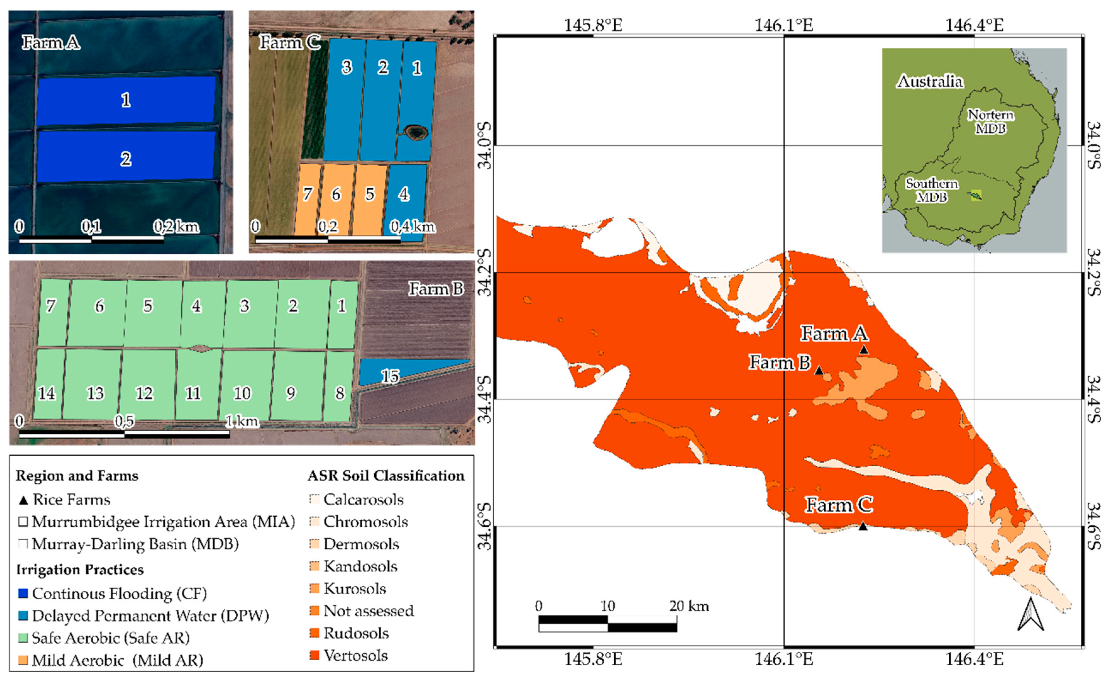
Figure 2.
Research methodology workflow.
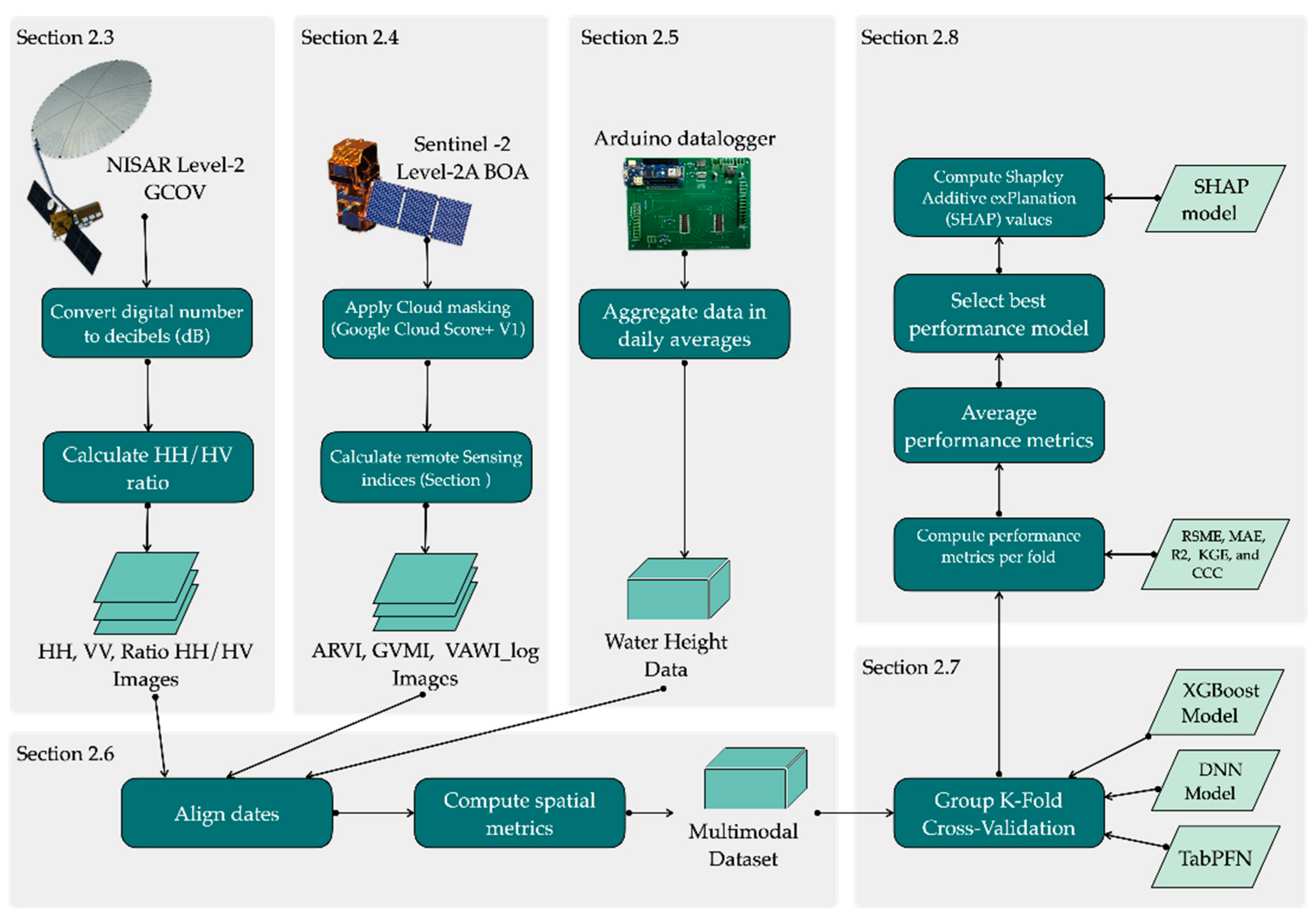
Figure 3.
Field inspection tube installation adapted from [40] (A), Schematic diagram for the calculation of the correction factor (cf) and Arduino datalogger with inspection tube field installation (C).
Figure 3.
Field inspection tube installation adapted from [40] (A), Schematic diagram for the calculation of the correction factor (cf) and Arduino datalogger with inspection tube field installation (C).
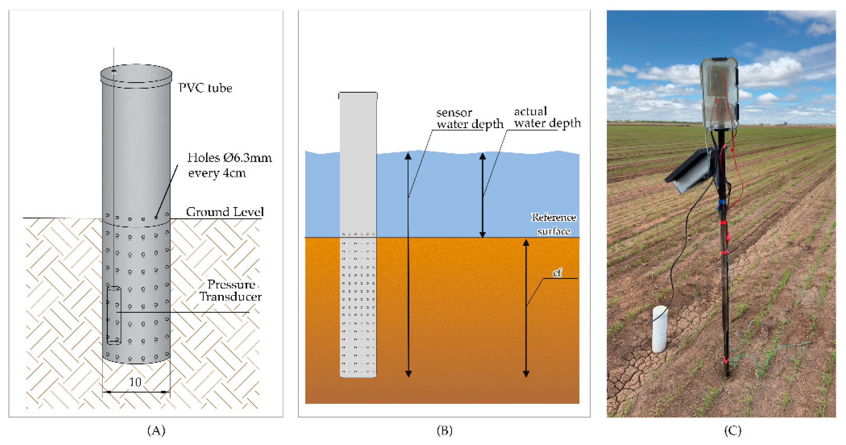
Figure 4.
Scatter plots of ML approaches estimated and observed water depth.
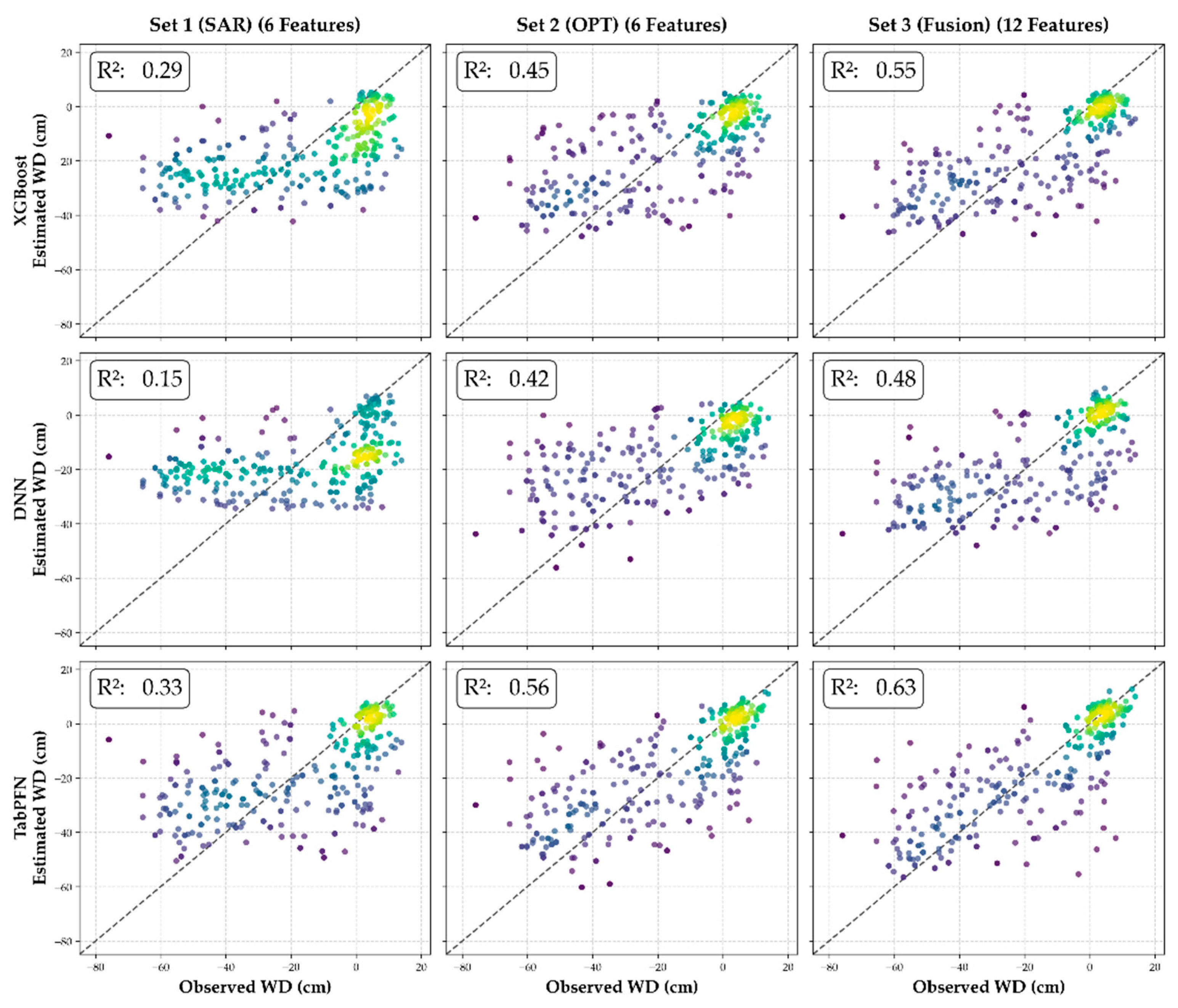
Figure 5.
TabPFN MAE error rate, crop growth and water height over crop period for CF (A), DPW (B), Safe AR (C), and mild AR (D).
Figure 5.
TabPFN MAE error rate, crop growth and water height over crop period for CF (A), DPW (B), Safe AR (C), and mild AR (D).
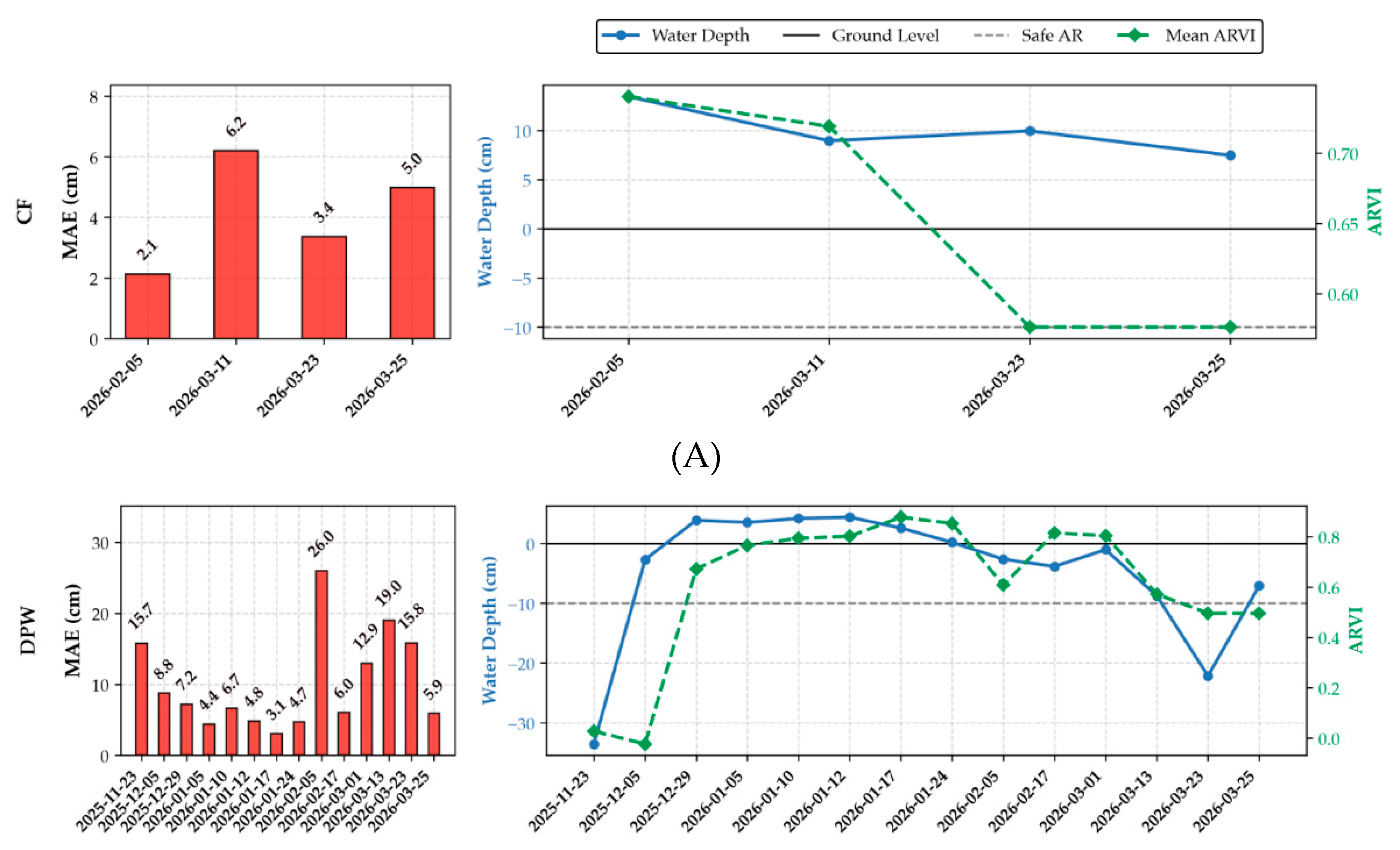
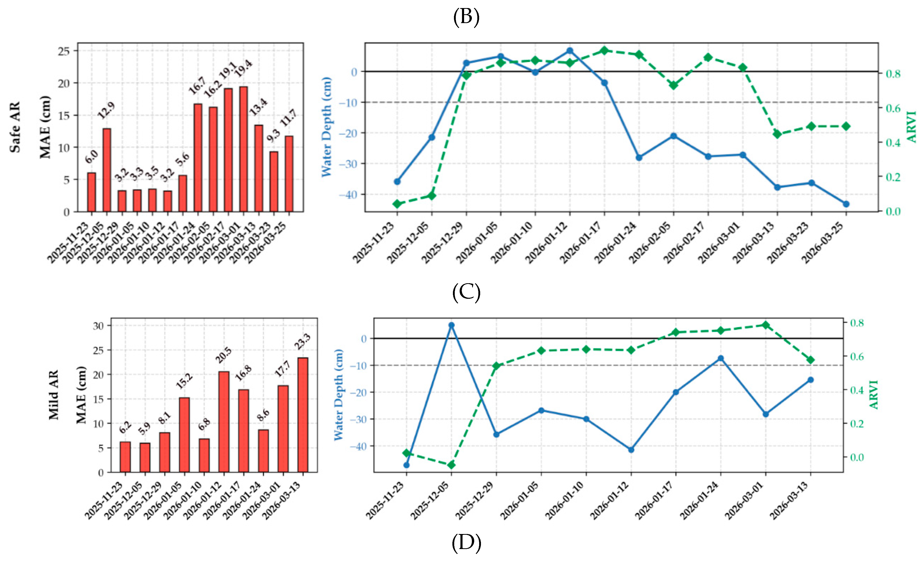
Figure 6.
SHAP values beehive plot (A) and mean |SHAP| values of each input feature of Set 3.
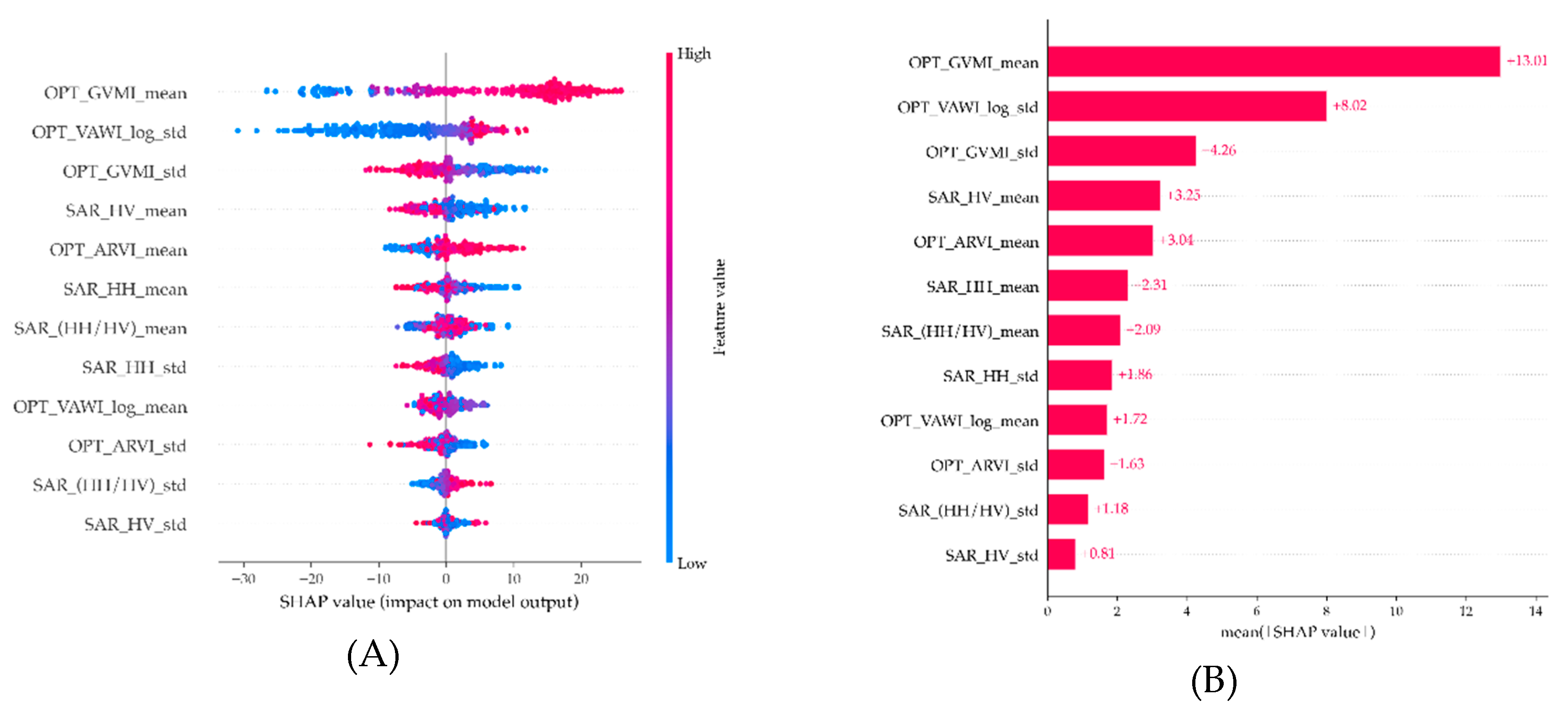
Figure 7.
Scatter plots of the SHAP values of mean (A), standard deviation (B), and mean (C).
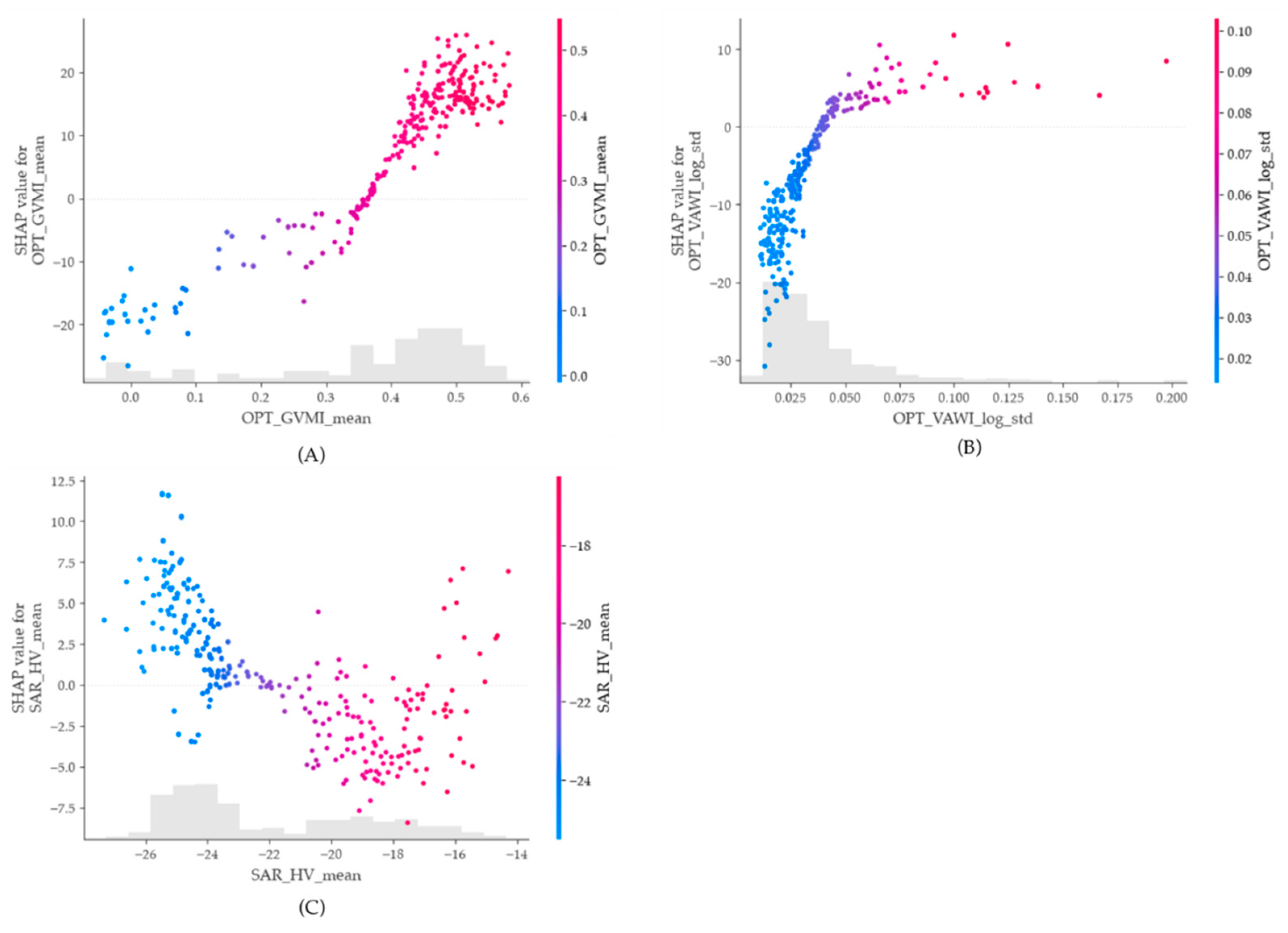
Figure 8.
Scatter plots of Water Heigh in relation to according to the standard deviation (A), and mean (B).
Figure 8.
Scatter plots of Water Heigh in relation to according to the standard deviation (A), and mean (B).
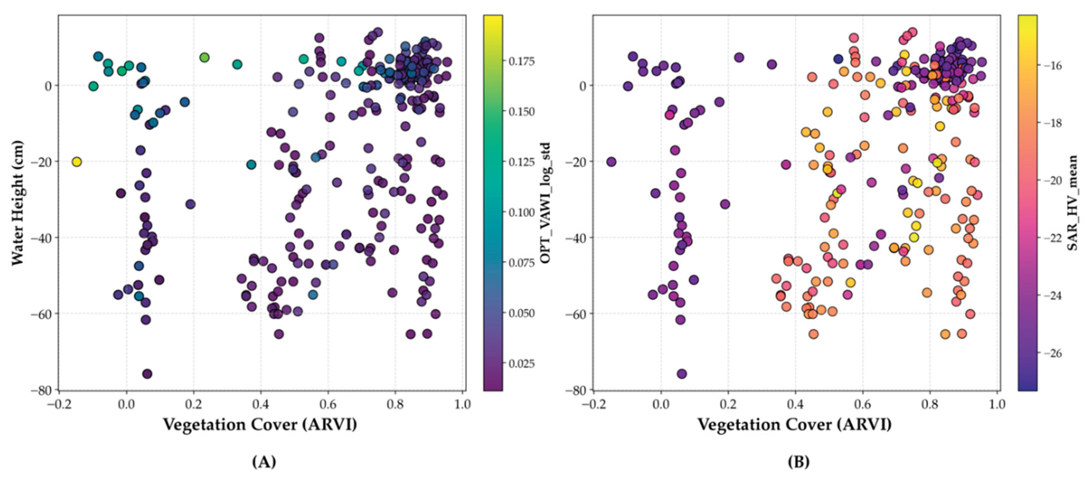

Table 1.
Optical remote sensing indices utilised in this research.
| Index | Formula | Reference |
|---|---|---|
| [36] | ||
| [37] | ||
| [38] | ||
| [39] | ||
| ) | [25] |
Table 2.
NISAR and Sentinel-2 acquisition date aliment.
| NISAR acquisition date | Sentinel-2 acquisition date | Acquisition date difference (days) |
|---|---|---|
| 23 November 2025 | 24 November 2025 | 1 |
| 5 December 2025 | 5 December 2025 | 0 |
| 29 December 2025 | 30 December 2025 | 1 |
| 5 January 2026 | 4 January 2026 | -1 |
| 7 January 2026 | 6 January 2026 | -1 |
| 10 January 2026 | 9 January 2026 | -1 |
| 12 January 2026 | 11 January 2026 | -1 |
| 17 January 2026 | 16 January 2026 | -1 |
| 24 January 2026 | 24 January 2026 | 0 |
| 5 February 2026 | 5 February 2026 | 0 |
| 17 February 2026 | 18 February 2026 | 1 |
| 1 March 2026 | 28 February 2026 | -1 |
| 11 March 2026 | 12 March 2026 | 1 |
| 13 March 2026 | 12 March 2026 | -1 |
| 23 March 2026 | 22 March 2026 | -1 |
| 25 March 2026 | 25 March 2026 | 0 |
Table 3.
Input features sets utilised to train each of the ML models.
| Input features | |
|---|---|
| Set 1 | HH_mean, HH_std, HV_mean, HV_std, (HH/HV)_mean, (HH/HV)_std |
| Set 2 | ARVI_mean, ARVI_std, GVMI_mean, GVMI_std, VAWI_log_mean, VAWI_log_std |
| Set 3 | HH_mean, HH_std, HV_mean, HV_std, (HH/HV)_mean, (HH/HV)_std, ARVI_mean, ARVI_std, GVMI_mean, GVMI_std, VAWI_log_mean, VAWI_log_std |
Table 4.
ML approaches result where (*) indicate the best metrics achieved by the models.
| Model | Feature Set | RMSE | MAE | KGE | CCC | |
|---|---|---|---|---|---|---|
| XGBoost | Set 1 | 19.63 | 15.94 | 0.29 | 0.32 | 0.43 |
| Set 2 | 17.22 | 13.53 | 0.45 | 0.52 | 0.61 | |
| Set 3 | 15.57* | 12* | 0.55* | 0.59* | 0.69* | |
| DNN | Set 1 | 21 | 16.94 | 0.18 | 0.2 | 0.32 |
| Set 2 | 17.19 | 13.52 | 0.45 | 0.46 | 0.59 | |
| Set 3 | 16.51* | 12.49* | 0.5* | 0.56* | 0.65* | |
| TabPFN | Set 1 | 18.98 | 14.23 | 0.33 | 0.49 | 0.55 |
| Set 2 | 15.49 | 11.64 | 0.56 | 0.65 | 0.72 | |
| Set 3 | 14.19* | 10.01* | 0.63* | 0.73* | 0.78* |
Disclaimer/Publisher’s Note: The statements, opinions and data contained in all publications are solely those of the individual author(s) and contributor(s) and not of MDPI and/or the editor(s). MDPI and/or the editor(s) disclaim responsibility for any injury to people or property resulting from any ideas, methods, instructions or products referred to in the content. |
© 2026 by the authors. Licensee MDPI, Basel, Switzerland. This article is an open access article distributed under the terms and conditions of the Creative Commons Attribution (CC BY) license (http://creativecommons.org/licenses/by/4.0/).
Copyright: This open access article is published under a Creative Commons CC BY 4.0 license, which permit the free download, distribution, and reuse, provided that the author and preprint are cited in any reuse.