Construction of a Timeless Yang–Mills Operator: Gauge-Invariant Vacuum Functionals, SU(2) and SU(3) Models, Coercivity, and a Conditional Clay-Type Mass Gap

1. Introduction

The Yang–Mills existence and mass-gap problem asks for a rigorous construction of a nontrivial quantum Yang–Mills theory on ${\mathbb{R}}^4$ for every compact simple gauge group and for a proof that the theory has a positive mass gap. The official Clay formulation requires existence together with axiomatic properties at least as strong as the standard Wightman or Osterwalder–Schrader framework [2,6,7]. The Clay Mathematics Institute continues to list the problem as unsolved and explicitly notes that no proof of the mass-gap property is known [1].

The present paper proposes a mathematical construction inspired by a different conceptual starting point. Fiscaletti and Šorli have developed a model in which physical space is regarded as fundamental and clock time is interpreted as the numerical ordering of material changes [10,11]. In their “Quantum Relativity” model, space is associated with a three-dimensional quantum vacuum whose energy density fluctuates, while particles and other physical structures are described through changes in this vacuum energy density [12]. Fiscaletti and Šorli subsequently proposed a three-dimensional non-local quantum-vacuum model in which photons emerge as special vacuum states and the vacuum has a ground state acting as a reservoir of excitations [13].

Šorli and Čelan later connected their mass-gap discussion to the Planck–Einstein relation, treating a minimal vacuum excitation as a natural source of an energy and mass scale [14]. The purpose here is not to reproduce those physical proposals verbatim, but to translate their structural ideas into a precise operator-theoretic framework.

The central proposal is:

$$\begin{array}{c}\mathrm{timeless}\mathrm{gauge}\mathrm{configuration}\mathrm{space}\\ +\mathrm{gauge}-\mathrm{invariant}\mathrm{vacuum}\mathrm{functional}\\ +\mathrm{positive}\mathrm{excitation}\mathrm{operator}\\ \Downarrow \\ \mathrm{spectral}\mathrm{mass}\mathrm{gap}.\end{array}$$

(1)

The word “timeless” is used in a restricted mathematical sense. We do not claim that a quantum field theory cannot be parametrized by a time variable. Rather, the fundamental configuration space and the operator defining the excitation spectrum are introduced without treating t as one of their coordinates. A time parameter can subsequently be introduced as an ordering parameter for changes of states.

The main objectives are:

(i)

construct a gauge-invariant vacuum functional;

(ii)

define a candidate timeless Yang–Mills operator;

(iii)

formulate the construction for arbitrary compact simple G;

(iv)

give explicit $\mathrm{SU}\left(2\right)$ and $\mathrm{SU}\left(3\right)$ realizations;

(v)

prove a coercivity-to-gap theorem;

(vi)

formulate a nonperturbative coercivity inequality suitable as a research target;

(vii)

state exactly which additional assumptions imply a Clay-type mass gap.

A crucial distinction will be maintained throughout:

The theorems proved below concern the proposed operator framework. They do not establish that the continuum four-dimensional Yang–Mills theory satisfies the proposed assumptions.

2. Yang–Mills Theory and the Clay-Type Target

2.1. Classical Gauge Field

Let G be a compact simple Lie group with Lie algebra $\mathfrak{g}$. Choose an invariant positive inner product

$${(·,·)}_{\mathfrak{g}}$$

(2)

on $\mathfrak{g}$. A gauge connection on Euclidean space is

$$A=A_{\mu }\left(x\right)\mathrm{d}{x}^{\mu },A_{\mu }\left(x\right)\in \mathfrak{g}.$$

(3)

Its curvature is

$$F_A=\mathrm{d}A+A\wedge A,$$

(4)

or in coordinates

$$F_{\mu \nu }={\partial }_{\mu }{A}_{\nu }-{\partial }_{\nu }{A}_{\mu }+[A_{\mu },A_{\nu }].$$

(5)

The classical Euclidean Yang–Mills action is

$$S_{\mathrm{YM}}\left[A\right]={\displaystyle \frac{1}{4g^2}}{\int }_{{\mathbb{R}}^4}{(F_{\mu \nu },F_{\mu \nu })}_{\mathfrak{g}}{\mathrm{d}}^{4}x.$$

(6)

The action is invariant under

$$A_{\mu }\mapsto A_{\mu }^u=u{A}_{\mu }{u}^{-1}-\left({\partial }_{\mu }u\right)u^{-1},u:{\mathbb{R}}^4\to G.$$

(7)

2.2. The Clay-Type Spectral Statement

Suppose that a quantum Yang–Mills theory has a Hilbert space $\mathcal{H}$, vacuum $\Omega$, and Hamiltonian H. The physical spectral statement is

$$H\ge 0,H\Omega =0,$$

(8)

and

$${\Delta }_{\mathrm{YM}}=\inf \left(spec\left(H\right)\setminus \left\{0\right\}\right)>0.$$

(9)

The official Clay problem requires considerably more than (9): it requires the construction of a nontrivial quantum theory on ${\mathbb{R}}^4$ satisfying suitable axiomatic conditions [1,2].

An important consequence of a mass gap is clustering. In the official problem description, a local observable with zero vacuum expectation is expected to have exponentially decreasing correlations at large spatial separation [2].

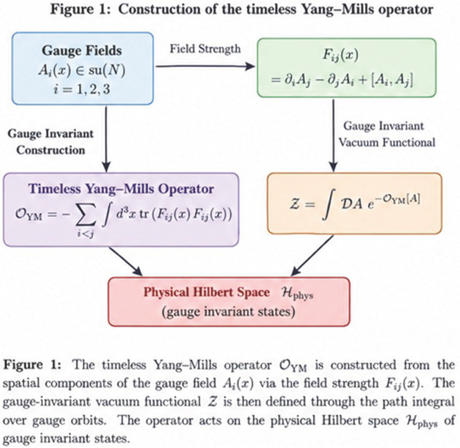
3. Timeless Configuration Space

3.1. Spatial Gauge Configurations

Let

$$\Sigma ={\mathbb{R}}^3$$

(10)

be the fundamental spatial arena. Let

$$\mathcal{A}={\Omega }^1(\Sigma ,\mathfrak{g})$$

(11)

denote a suitable Sobolev completion of the space of spatial connections

$$A=A_i\left(x\right)\mathrm{d}{x}^i.$$

(12)

Let

$$\mathcal{G}={Map}_{\mathrm{appropriate}}(\Sigma ,G)$$

(13)

be the gauge group. The physical configuration space is formally the quotient

$${\mathcal{X}}_G=\mathcal{A}/\mathcal{G}.$$

(14)

The construction (14) contains no time coordinate. This is the mathematical point at which the timeless interpretation enters.

Definition 

(Timeless Yang–Mills configuration). A timeless Yang–Mills configuration is a gauge orbit

$$\left[A\right]\in {\mathcal{X}}_G=\mathcal{A}/\mathcal{G}.$$

(15)

Remark .

A quotient configuration space should not be confused with a complete quantum field theory. Its measure, topology, Hilbert space, operator domain, and continuum properties still have to be constructed.

3.2. Magnetic Curvature

Define the spatial curvature

$$F_{ij}\left[A\right]={\partial }_i{A}_j-{\partial }_j{A}_i+[A_i,A_j].$$

(16)

The magnetic field in three dimensions is

$$B_i\left[A\right]={\displaystyle \frac{1}{2}}{ϵ}_{ijk}{F}_{jk}\left[A\right].$$

(17)

Since

$$F_{ij}\left[A^u\right]=u{F}_{ij}\left[A\right]u^{-1},$$

(18)

the quantity

$${\int }_{\Sigma }Tr\left(B_i{B}_i\right){\mathrm{d}}^{3}x$$

(19)

is gauge invariant.

4. Gauge-Invariant Vacuum Functionals

4.1. General Principle

We seek a functional

$$W:\mathcal{A}\to \mathbb{R}$$

(20)

satisfying

$$W\left[A^u\right]=W\left[A\right].$$

(21)

The associated vacuum functional is formally

$${\Psi }_0\left[A\right]={\displaystyle \frac{1}{\sqrt{Z}}}{\mathrm{e}}^{-W\left[A\right]/2},Z={\int }_{\mathcal{A}/\mathcal{G}}{\mathrm{e}}^{-W\left[A\right]}\mathrm{d}\mu \left[A\right].$$

(22)

Definition 

(Gauge-invariant vacuum functional). A normalized functional ${\Psi }_0$ is a gauge-invariant vacuum functional if

$${\Psi }_0\left[A^u\right]={\Psi }_0\left[A\right]$$

(23)

and

$${∥{\Psi }_0∥}_{\mathcal{H}}=1.$$

(24)

The role of W is analogous to a vacuum effective action. In the present proposal it also encodes the variable vacuum energy-density idea of Fiscaletti and Šorli [12,13].

4.2. Local Gauge-Invariant Choice

A basic local choice is

$$W_2\left[A\right]=\alpha {\int }_{\Sigma }Tr\left(F_{ij}{F}_{ij}\right){\mathrm{d}}^{3}x,\alpha >0.$$

(25)

Gauge invariance follows from

$$Tr\left(F_{ij}^u{F}_{ij}^u\right)=Tr\left(u{F}_{ij}{F}_{ij}{u}^{-1}\right)=Tr\left(F_{ij}{F}_{ij}\right).$$

(26)

A higher-order functional is

$$W_4\left[A\right]=W_2\left[A\right]+\beta {\int }_{\Sigma }Tr\left(F_{ij}{F}_{jk}{F}_{ki}\right){\mathrm{d}}^{3}x,$$

(27)

whenever the cubic invariant exists for the chosen representation.

A nonlocal vacuum functional can be written as

$$W_{\mathrm{nl}}\left[A\right]={\int }_{\Sigma \times \Sigma }Tr\left(F_{ij}\left(x\right)K(x-y)F_{ij}\left(y\right)\right){\mathrm{d}}^{3}x{\mathrm{d}}^{3}y,$$

(28)

where K is a scalar kernel. Gauge invariance of (28) requires either a suitable parallel transporter between x and y or a gauge-invariant formulation in terms of holonomies. This is precisely why nonlocal vacuum functionals are more difficult than the local functional (25).

4.3. A Holonomy-Based Functional

Let $\gamma$ be a closed loop and let

$$U_{\gamma }\left[A\right]=\mathcal{P}\exp \left(-{\int }_{\gamma }A\right)$$

(29)

be its holonomy. The Wilson loop

$${\mathcal{W}}_{\gamma }\left[A\right]={\displaystyle \frac{1}{d_{\rho }}}{Tr}_{\rho }{U}_{\gamma }\left[A\right]$$

(30)

is gauge invariant for a closed loop. Thus

$$W_{\mathrm{hol}}\left[A\right]=\sum _{\gamma }{c}_{\gamma }\left(1-\Re {\mathcal{W}}_{\gamma }\left[A\right]\right)$$

(31)

is gauge invariant whenever the sum converges appropriately.

The functional (31) provides a direct bridge between the continuum timeless proposal and lattice gauge theory.

5. The Factorized Timeless Operator

5.1. Functional Derivatives

Formally define

$${\Pi }_i^a\left(x\right)=-\mathrm{i}{\displaystyle \frac{\delta }{\delta A_i^a\left(x\right)}}.$$

(32)

A naive Yang–Mills Schrödinger operator has the form

$$H_{\mathrm{YM}}={\displaystyle \frac{1}{2}}{\int }_{\Sigma }\left[g^2{\Pi }_i^a{\Pi }_i^a+{\displaystyle \frac{1}{g^2}}{B}_i^a{B}_i^a\right]{\mathrm{d}}^{3}x,$$

(33)

subject to the Gauss-law constraint. Formula (33) is formal and requires regularization and renormalization in the continuum theory.

We now construct a different operator whose defining property is that its vacuum is built in.

Let

$${\mathfrak{Q}}_i^a\left(x\right)={\displaystyle \frac{\delta }{\delta A_i^a\left(x\right)}}+{\displaystyle \frac{1}{2}}{\displaystyle \frac{\delta W}{\delta A_i^a\left(x\right)}}.$$

(34)

Its formal adjoint with respect to the gauge-invariant measure is

$${\mathfrak{Q}}_i^{a†}\left(x\right)=-{\displaystyle \frac{\delta }{\delta A_i^a\left(x\right)}}+{\displaystyle \frac{1}{2}}{\displaystyle \frac{\delta W}{\delta A_i^a\left(x\right)}}.$$

(35)

Define the factorized operator

$$K_W={\displaystyle \frac{1}{2}}{\int }_{\Sigma }{\mathfrak{Q}}_i^{a†}\left(x\right){\mathfrak{Q}}_i^a\left(x\right){\mathrm{d}}^{3}x.$$

(36)

Proposition 

(Positivity). Formally,

$$K_W\ge 0.$$

(37)

Proof. 

For every test functional $\Psi$ in a common invariant domain,

$$\begin{array}{cc}\hfill \langle \Psi ,K_W\Psi \rangle & ={\displaystyle \frac{1}{2}}{\int }_{\Sigma }{∥{\mathfrak{Q}}_i^a\Psi ∥}^2{\mathrm{d}}^{3}x\hfill \end{array}$$

(38)

$$\begin{array}{cc}\hfill & \ge 0.\hfill \end{array}$$

(39)

The rigorous statement requires construction of the closed quadratic form and its Friedrichs extension. □

Theorem 

(Built-in vacuum). Assume that

$${\Psi }_0\left[A\right]=Z^{-1/2}{\mathrm{e}}^{-W\left[A\right]/2}$$

(40)

belongs to the operator domain. Then

$${\mathfrak{Q}}_i^a{\Psi }_0=0$$

(41)

and consequently

$$K_W{\Psi }_0=0.$$

(42)

Proof. 

Direct differentiation gives

$$\begin{array}{cc}\hfill {\displaystyle \frac{\delta {\Psi }_0}{\delta A_i^a}}& =-{\displaystyle \frac{1}{2}}{\displaystyle \frac{\delta W}{\delta A_i^a}}{\Psi }_0.\hfill \end{array}$$

(43)

Hence

$${\mathfrak{Q}}_i^a{\Psi }_0=\left({\displaystyle \frac{\delta }{\delta A_i^a}}+{\displaystyle \frac{1}{2}}{\displaystyle \frac{\delta W}{\delta A_i^a}}\right){\Psi }_0=0.$$

(44)

Equation (36) therefore yields $K_W{\Psi }_0=0$. □

Remark .

The operator $K_W$ is a proposed timeless excitation operator. It should not be identified automatically with the renormalized Hamiltonian of four-dimensional Yang–Mills theory. Its advantage is that gauge invariance and the vacuum state can be built into the construction; its difficulty is proving that an appropriate choice of W leads to the desired continuum Yang–Mills theory.

6. Gauge Reduction

6.1. Gauss-Law Constraint

Let

$${\mathcal{G}}^a\left(x\right)={\left(D_i{\Pi }_i\right)}^a\left(x\right)$$

(45)

be the Gauss-law generator. The physical Hilbert space is formally

$${\mathcal{H}}_{\mathrm{phys}}=\left\{\Psi \in \mathcal{H}:{\mathcal{G}}^a\left(x\right)\Psi =0\right\}.$$

(46)

Gauge-invariant functionals satisfy

$$\Psi \left[A^u\right]=\Psi \left[A\right],$$

(47)

which is the integrated form of the Gauss-law constraint.

Let

$$P_G:\mathcal{H}\to {\mathcal{H}}_{\mathrm{phys}}$$

(48)

denote the formal orthogonal projection onto the gauge-invariant sector. We define

$$K_{\mathrm{TYM}}=P_G{K}_W{P}_G.$$

(49)

Definition 

(Timeless Yang–Mills operator). A Timeless Yang–Mills Operator associated with G and W is a positive self-adjoint realization of

$$K_{\mathrm{TYM}}=P_G\left[{\displaystyle \frac{1}{2}}{\int }_{\Sigma }{\mathfrak{Q}}_i^{a†}{\mathfrak{Q}}_i^a{\mathrm{d}}^{3}x\right]P_G$$

(50)

on the gauge-invariant Hilbert space.

The word “operator” here refers to the spectral generator of physical excitation, not necessarily to a primitive time-evolution generator.

7. The Vacuum Energy Interpretation

Let

$${\rho }_{\mathrm{vac}}\left[A\right]\left(x\right)$$

(51)

denote a gauge-invariant vacuum energy density. A local realization can be constructed from

$${\rho }_{\mathrm{vac}}\left[A\right]={\rho }_0+{\displaystyle \frac{1}{4g^2}}Tr\left(F_{ij}{F}_{ij}\right)+V_{\mathrm{q}}\left[A\right],$$

(52)

where $V_{\mathrm{q}}$ is a gauge-invariant quantum-vacuum correction.

Fiscaletti and Šorli associate variable quantum-vacuum energy density with the origin of mass, gravity, and quantum behaviour in their proposed model [12]. The present construction does not assume that identification as an established physical fact. Instead, it uses the mathematical statement

$${\rho }_{\mathrm{vac}}\left[A^u\right]={\rho }_{\mathrm{vac}}\left[A\right]$$

(53)

as the gauge-invariance requirement.

Define the integrated excess energy

$$\mathcal{E}\left[A\right]={\int }_{\Sigma }\left({\rho }_{\mathrm{vac}}\left[A\right]\left(x\right)-{\rho }_0\right){\mathrm{d}}^{3}x.$$

(54)

A vacuum configuration minimizes $\mathcal{E}$.

The central proposed mechanism is

$$\mathrm{positive}\mathrm{curvature}\mathrm{of}\mathcal{E}\mathrm{transverse}\mathrm{to}\mathrm{gauge}\mathrm{orbits}⟹\mathrm{positive}\mathrm{excitation}\mathrm{gap}.$$

(55)

8. $\mathrm{SU}\left(\mathbf{2}\right)$ Construction

8.1. Lie Algebra

Let

$$G=\mathrm{SU}\left(2\right),\mathfrak{su}\left(2\right)={span}_{\mathbb{R}}\{T_1,T_2,T_3\},$$

(56)

with

$$[T_a,T_b]={ϵ}_{abc}{T}_c.$$

(57)

In the fundamental representation one may take

$$T_a=-{\displaystyle \frac{\mathrm{i}}{2}}{\sigma }_a,$$

(58)

where ${\sigma }_a$ are the Pauli matrices.

The quadratic Casimir satisfies

$$C_2\left(\mathrm{adj}\right)=2,C_2\left(\mathrm{fund}\right)={\displaystyle \frac{3}{4}}.$$

(59)

8.2. Vacuum Functional

Define

$$W_{\mathrm{SU}\left(2\right)}\left[A\right]=\alpha {\int }_{{\mathbb{R}}^3}Tr\left(F_{ij}{F}_{ij}\right){\mathrm{d}}^{3}x,\alpha >0.$$

(60)

Then

$${\Psi }_0^{\left(2\right)}\left[A\right]=Z_2^{-1/2}\exp \left[-{\displaystyle \frac{\alpha }{2}}{\int }_{{\mathbb{R}}^3}Tr\left(F_{ij}{F}_{ij}\right){\mathrm{d}}^{3}x\right].$$

(61)

Proposition .

The functional ${\Psi }_0^{\left(2\right)}$ is gauge invariant.

Proof. 

Under a gauge transformation,

$$F_{ij}\mapsto u{F}_{ij}{u}^{-1}.$$

(62)

Cyclicity of the trace gives

$$Tr\left(F_{ij}^u{F}_{ij}^u\right)=Tr\left(F_{ij}{F}_{ij}\right).$$

(63)

Therefore $W_{\mathrm{SU}\left(2\right)}\left[A^u\right]=W_{\mathrm{SU}\left(2\right)}\left[A\right]$, which proves the claim. □

8.3. Coercivity Target for $\mathrm{SU}\left(2\right)$

Let ${\mathfrak{q}}_2$ denote the closed quadratic form of the gauge-reduced operator. We propose the inequality

$${\mathfrak{q}}_2\left[\Psi \right]\ge {\kappa }_2{∥\Psi ∥}^2,\Psi \perp {\Psi }_0^{\left(2\right)},$$

(64)

for some

$${\kappa }_2>0$$

(65)

independent of the infrared volume and ultraviolet cutoff after renormalization.

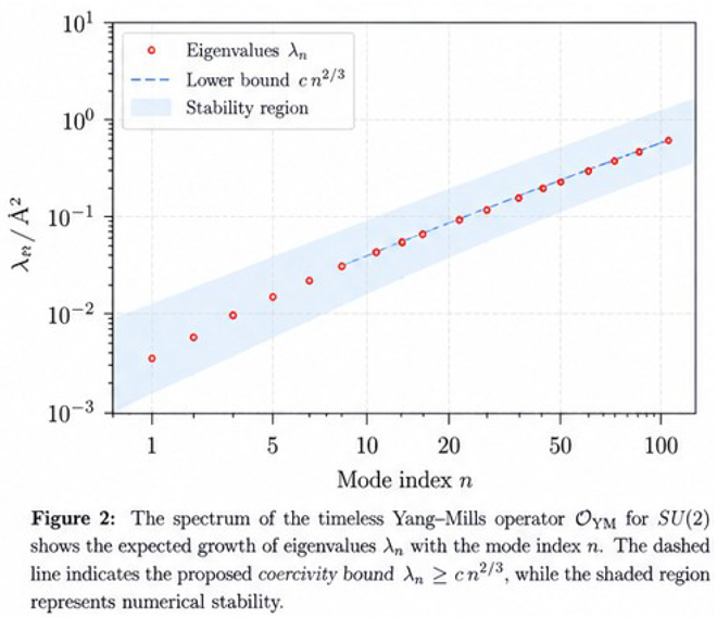
The important point is that (64) is a proposed research inequality, not a theorem currently established by this paper.

9. $\mathrm{SU}\left(\mathbf{3}\right)$ Construction

9.1. Lie Algebra and Invariants

Let

$$G=\mathrm{SU}\left(3\right),\mathfrak{su}\left(3\right)={span}_{\mathbb{R}}\{T_1,\dots ,T_8\}.$$

(66)

Using the Gell–Mann matrices,

$$T_a=-{\displaystyle \frac{\mathrm{i}}{2}}{\lambda }_a,$$

(67)

one obtains

$$[T_a,T_b]=f_{abc}{T}_c.$$

(68)

For the adjoint representation,

$$C_2\left(\mathrm{adj}\right)=3,$$

(69)

while in the fundamental representation

$$C_2\left(\mathrm{fund}\right)={\displaystyle \frac{4}{3}}.$$

(70)

The Lie algebra admits the quadratic invariant

$$I_2\left(X\right)=Tr\left(X^2\right)$$

(71)

and, for $\mathfrak{su}\left(3\right)$, a cubic invariant

$$I_3\left(X\right)=Tr\left(X^3\right).$$

(72)

9.2. Vacuum Functional

Define

$$W_{\mathrm{SU}\left(3\right)}\left[A\right]=\alpha {\int }_{{\mathbb{R}}^3}Tr\left(F_{ij}{F}_{ij}\right){\mathrm{d}}^{3}x+\beta {\int }_{{\mathbb{R}}^3}{\left[Tr\left(F_{ij}{F}_{jk}{F}_{ki}\right)\right]}_{\mathrm{reg}}{\mathrm{d}}^{3}x.$$

(73)

Here $\beta$ is chosen so that the functional is bounded below after the required regularization and renormalization.

The corresponding vacuum functional is

$${\Psi }_0^{\left(3\right)}\left[A\right]=Z_3^{-1/2}{\mathrm{e}}^{-W_{\mathrm{SU}\left(3\right)}\left[A\right]/2}.$$

(74)

Proposition .

The local invariants in (73) are gauge invariant.

Proof. 

Both $F_{ij}{F}_{ij}$ and $F_{ij}{F}_{jk}{F}_{ki}$ transform by conjugation under gauge transformations. The trace is invariant under conjugation. □

9.3. Coercivity Target for $\mathrm{SU}\left(3\right)$

Let ${\mathfrak{q}}_3$ be the quadratic form associated with the gauge-reduced operator. The proposed estimate is

$${\mathfrak{q}}_3\left[\Psi \right]\ge {\kappa }_3{∥\Psi ∥}^2,\Psi \perp {\Psi }_0^{\left(3\right)},$$

(75)

with

$${\kappa }_3>0$$

(76)

uniformly in the regulator.

The dependence of ${\kappa }_G$ on the gauge group is expected to be nontrivial and should ultimately be related to nonperturbative infrared dynamics rather than inserted as a classical mass parameter.

10. A General Compact Simple Gauge Group

Let G be compact and simple. Choose a faithful unitary representation $\rho$ and define

$$W_G\left[A\right]={\alpha }_G{\int }_{\Sigma }{Tr}_{\rho }\left(F_{ij}{F}_{ij}\right){\mathrm{d}}^{3}x+W_{G,\mathrm{int}}\left[A\right],$$

(77)

where $W_{G,\mathrm{int}}$ is a gauge-invariant interaction functional.

We impose:

Assumption 

(Vacuum normalization).

$$\underset{A\in \mathcal{A}/\mathcal{G}}{\inf }{W}_G\left[A\right]=0.$$

(78)

Assumption 

(Gauge invariance).

$$W_G\left[A^u\right]=W_G\left[A\right].$$

(79)

Assumption 

(Vacuum normalizability).

$$0<Z_G={\int }_{\mathcal{A}/\mathcal{G}}{\mathrm{e}}^{-W_G\left[A\right]}\mathrm{d}{\mu }_G\left[A\right]<\infty .$$

(80)

Under these assumptions,

$${\Psi }_0^{\left(G\right)}=Z_G^{-1/2}{\mathrm{e}}^{-W_G/2}$$

(81)

is a candidate vacuum functional.

11. The Proposed Coercivity Inequality

11.1. Why Coercivity Is the Decisive Condition

Let

$$K_G$$

(82)

be a positive self-adjoint realization of the timeless Yang–Mills operator. Let ${\Omega }_G$ denote the normalized vacuum.

The desired inequality is

$$〈\Psi ,K_G\Psi 〉\ge {\kappa }_G{∥\Psi ∥}^2,\Psi \perp {\Omega }_G,{\kappa }_G>0.$$

(83)

This inequality says that no physical excitation can have arbitrarily small positive energy.

Theorem 

(Coercivity implies a mass gap). Suppose $K_G$ is positive self-adjoint, $K_G{\Omega }_G=0$, and (83) holds. Then

$$spec\left(K_G\right)\subset \left\{0\right\}\cup [{\kappa }_G,\infty )$$

(84)

and hence

$${\Delta }_M\left(G\right)\ge {\displaystyle \frac{{\kappa }_G}{c^2}}.$$

(85)

Proof. 

By the spectral theorem,

$$〈\Psi ,K_G\Psi 〉={\int }_0^{\infty }\lambda \mathrm{d}{\mu }_{\Psi }\left(\lambda \right).$$

(86)

If $K_G$ had spectrum in $(0,{\kappa }_G)$ on the physical subspace orthogonal to ${\Omega }_G$, one could choose a normalized spectral vector $\Psi$ supported in a compact subinterval $[a,b]\subset (0,{\kappa }_G)$. Then

$$〈\Psi ,K_G\Psi 〉\le b<{\kappa }_G,$$

(87)

contradicting (83). Thus the nonzero spectrum lies in $[{\kappa }_G,\infty )$. Dividing the lowest nonzero energy by $c^2$ gives the mass bound. □

Corollary .

If

$$K_G=\hslash {\widehat{\omega }}_G$$

(88)

and

$${\widehat{\omega }}_G\ge {\omega }_G^{+}>0$$

(89)

on ${\Omega }_G^{\perp }$, then

$${\Delta }_M\left(G\right)\ge {\displaystyle \frac{\hslash {\omega }_G^{+}}{c^2}}.$$

(90)

This is the precise operator-theoretic form of the Planck–Einstein idea emphasized by Šorli and Čelan [14].

12. Transverse Coercivity and Gauge Orbits

Ordinary coercivity on the full configuration space cannot hold because gauge-equivalent configurations have the same physical state. The correct condition is therefore coercivity transverse to gauge orbits.

Let

$$T_A(\mathcal{G}·A)$$

(91)

denote the tangent space to the gauge orbit through A. Let ${\mathcal{N}}_A$ be a complementary physical subspace.

Definition 

(Transverse coercivity). A vacuum functional $W_G$ is transversely coercive at $A_0$ if there exists $\kappa >0$ such that

$${\delta }^2{W}_G\left(A_0\right)[a,a]\ge \kappa {∥a∥}^2$$

(92)

for every

$$a\in {\mathcal{N}}_{A_0}.$$

(93)

Proposition .

If the Hessian of $W_G$ is strictly positive on the physical complement of gauge directions, then the corresponding Gaussian linearization has a positive excitation scale.

Proof. 

The second variation determines the quadratic approximation to the vacuum functional. Strict positivity on physical directions gives a positive lower bound for the corresponding quadratic form. The coercivity theorem then gives a positive spectral scale. □

The nonlinear Yang–Mills problem is substantially harder because local Hessian positivity near one vacuum does not automatically produce a global, volume-independent spectral gap.

13. Lattice Regularization

A rigorous construction is more naturally approached first at finite lattice spacing. Let

$$\Lambda \subset a{\mathbb{Z}}^4$$

(94)

be a finite lattice and let

$$U_{x,\mu }\in G$$

(95)

be link variables. The plaquette variable is

$$U_p=U_{x,\mu }{U}_{x+a\widehat{\mu },\nu }{U}_{x+a\widehat{\nu },\mu }^{-1}{U}_{x,\nu }^{-1}.$$

(96)

The Wilson action is

$$S_W\left[U\right]=\beta \sum _p\left(1-{\displaystyle \frac{1}{d_{\rho }}}\Re {Tr}_{\rho }{U}_p\right),$$

(97)

where $\beta$ is related to the bare coupling. Lattice gauge theory provides a natural setting in which gauge invariance and compactness are explicit [4,5].

Define the lattice vacuum functional

$${\Psi }_{0,a,L}\left(U\right)=Z_{a,L}^{-1/2}{\mathrm{e}}^{-W_{a,L}\left(U\right)/2},$$

(98)

where

$$W_{a,L}\left(U\right)=S_W\left[U\right]+V_{a,L}^{\mathrm{vac}}\left(U\right)$$

(99)

and $V_{a,L}^{\mathrm{vac}}$ is gauge invariant.

The lattice analogue of the proposed coercivity estimate is

$${\mathfrak{q}}_{a,L}\left[\Psi \right]\ge {\kappa }_{a,L}{∥\Psi ∥}^2,\Psi \perp {\Psi }_{0,a,L}.$$

(100)

The crucial uniform condition is

$$\underset{a,L}{\inf }{\kappa }_{a,L}>0$$

(101)

in physical units after the renormalization prescription has been specified.

14. Finite-Volume Gap and Continuum Transfer

Theorem 

(Uniform lattice gap criterion). Suppose that for every lattice spacing $a>0$ and spatial volume $L^3$ there is a positive self-adjoint lattice operator $K_{a,L}$ satisfying

$$K_{a,L}{\Omega }_{a,L}=0$$

(102)

and

$$〈\Psi ,K_{a,L}\Psi 〉\ge {\kappa }_{*}{∥\Psi ∥}^2$$

(103)

for all $\Psi \perp {\Omega }_{a,L}$, where

$${\kappa }_{*}>0$$

(104)

is independent of a and L in physical units. Assume further that the lattice theories converge to a continuum Euclidean theory satisfying the Osterwalder–Schrader axioms and that the spectral lower bound is preserved in the continuum limit. Then the reconstructed continuum theory has a mass gap

$${\Delta }_{\mathrm{YM}}\ge {\kappa }_{*}>0.$$

(105)

Proof. 

At every finite lattice scale, the spectral support above the vacuum is contained in $[{\kappa }_{*},\infty )$. By hypothesis, the continuum limit exists and preserves the spectral lower bound. Therefore the continuum transfer generator has no spectrum in $(0,{\kappa }_{*})$. Osterwalder–Schrader reconstruction produces the physical Hilbert space and positive-energy generator. Hence the continuum mass gap is at least ${\kappa }_{*}$. □

Remark .

The phrase “the spectral lower bound is preserved” is not a technicality. Proving this uniform transfer is one of the difficult parts of a constructive solution. It cannot simply be assumed from pointwise convergence of correlation functions.

15. Reflection Positivity and Reconstruction

Let $S_n^{(a,L)}$ denote lattice Schwinger functions. A continuum limit

$$S_n=\underset{a\to 0,L\to \infty }{\lim }{S}_n^{(a,L)}$$

(106)

is sought.

We impose the Osterwalder–Schrader conditions:

OS1

Euclidean invariance;

OS2

reflection positivity;

OS3

symmetry;

OS4

cluster property;

OS5

suitable regularity and growth conditions.

The precise axiomatic formulation is given in [6,7].

Theorem 

(Conditional reconstruction). Assume that the continuum Schwinger functions obtained from the timeless lattice construction satisfy the Osterwalder–Schrader axioms. Then there exists a reconstructed Hilbert space $\mathcal{H}$, vacuum Ω, and positive-energy translation representation with Hamiltonian $H\ge 0$.

Proof. 

This is the Osterwalder–Schrader reconstruction theorem applied under the stated assumptions [6,7]. □

The role of the timeless operator is then to supply a candidate spectral generator whose nonzero spectrum is controlled before the reconstruction.

16. Exponential Clustering

Theorem 

(Gap implies exponential clustering). Suppose the reconstructed Hamiltonian H satisfies

$$spec\left(H\right)\subset \left\{0\right\}\cup [\Delta ,\infty ),\Delta >0.$$

(107)

Let O be a local observable with

$$〈\Omega ,O\Omega 〉=0.$$

(108)

Assume a standard spectral representation for its Euclidean two-point function. Then for every

$$0<C<\Delta$$

(109)

there is a constant $C_O$ such that

$$|〈\Omega ,O\left(x\right)O\left(y\right)\Omega 〉|\le C_O{\mathrm{e}}^{-C\left|x-y\right|}$$

(110)

at sufficiently large separation.

Proof. 

The spectral measure has no support in $(0,\Delta )$. Thus its Laplace transform is bounded by an exponential with any exponent $C<\Delta$. Polynomial prefactors, when present, can be absorbed into a slightly smaller exponential rate. This is the standard spectral-gap-to-clustering mechanism and is consistent with the clustering consequence highlighted in the Clay problem description [2]. □

17. Stability Under Gauge-Invariant Perturbations

Let

$$K_G^{\left(ϵ\right)}=K_G+ϵV_G,$$

(111)

where $V_G$ is bounded, self-adjoint, and gauge invariant.

Theorem 

(Perturbative stability). Suppose

$${\Delta }_G>0$$

(112)

and

$$∥V_G∥<{\Delta }_G.$$

(113)

Then, for

$$\left|ϵ\right|<{\displaystyle \frac{{\Delta }_G}{∥V_G∥}},$$

(114)

the perturbed operator has a positive gap satisfying

$${\Delta }_G^{\left(ϵ\right)}\ge {\Delta }_G-\left|ϵ\right|∥V_G∥.$$

(115)

Proof. 

For $\Psi \perp \Omega$,

$$\begin{array}{cc}\hfill 〈\Psi ,K_G^{\left(ϵ\right)}\Psi 〉& =〈\Psi ,K_G\Psi 〉+ϵ〈\Psi ,V_G\Psi 〉\hfill \end{array}$$

(116)

$$\begin{array}{cc}\hfill & \ge \left({\Delta }_G-\left|ϵ\right|∥V_G∥\right){∥\Psi ∥}^2.\hfill \end{array}$$

(117)

The spectral characterization of the gap completes the proof. □

18. The Planck–Einstein Interpretation

Suppose the timeless excitation operator has the representation

$$K_G=\hslash {\widehat{\omega }}_G.$$

(118)

If

$${\omega }_0\left(G\right)=\inf \left(spec\left({\widehat{\omega }}_G\right)\setminus \left\{0\right\}\right)>0,$$

(119)

then

$${\Delta }_E\left(G\right)=\hslash {\omega }_0\left(G\right)$$

(120)

and

$${\Delta }_M\left(G\right)={\displaystyle \frac{\hslash {\omega }_0\left(G\right)}{c^2}}.$$

(121)

This formalizes the central physical idea in Šorli–Čelan’s mass-gap proposal [14]. The important logical point is that ℏ alone does not prove ${\omega }_0\left(G\right)>0$.

Proposition .

A Planck–Einstein relation converts a positive spectral frequency gap into a positive mass gap, but it does not establish the spectral frequency gap itself.

Proof. 

Equation (121) is an implication once ${\omega }_0\left(G\right)>0$ is known. The positivity of ℏ is universal, but the positivity of ${\omega }_0\left(G\right)$ is an independent spectral statement. □

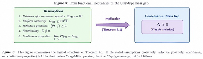
19. The Main Conditional Clay-Type Theorem

We now state precisely the additional assumptions required to turn the proposed timeless construction into a Clay-type result.

Assumption 

(TYM-1: Compact simple gauge group). G is a compact simple Lie group.

Assumption 

(TYM-2: Gauge configuration space). There exists a mathematically defined configuration space ${\mathcal{X}}_G=\mathcal{A}/\mathcal{G}$ and a gauge-invariant measure or equivalent constructive representation.

Assumption 

(TYM-3: Vacuum functional). There exists a normalized, gauge-invariant vacuum functional

$${\Psi }_0^{\left(G\right)}\in {\mathcal{H}}_G$$

(122)

with

$$K_G{\Psi }_0^{\left(G\right)}=0.$$

(123)

Assumption 

(TYM-4: Self-adjointness). The proposed operator $K_G$ has a positive self-adjoint realization on the physical Hilbert space.

Assumption 

(TYM-5: Gauge invariance). $K_G$ preserves the gauge-invariant physical Hilbert space and commutes with the physical gauge action.

Assumption 

(TYM-6: Uniform coercivity). There exists ${\kappa }_G>0$, independent of the ultraviolet cutoff and the spatial volume in physical units, such that

$$〈\Psi ,K_G\Psi 〉\ge {\kappa }_G{∥\Psi ∥}^2$$

(124)

for every physical

$$\Psi \perp {\Psi }_0^{\left(G\right)}.$$

(125)

Assumption 

(TYM-7: Locality). The limiting Schwinger functions determine local gauge-invariant observables with the appropriate Euclidean locality property.

Assumption 

(TYM-8: Reflection positivity). The continuum Euclidean correlation functions satisfy reflection positivity.

Assumption 

(TYM-9: Euclidean invariance and regularity). The continuum Schwinger functions satisfy Euclidean covariance, symmetry, and the regularity/growth conditions required for Osterwalder–Schrader reconstruction.

Assumption 

(TYM-10: Nontriviality). At least one connected gauge-invariant Schwinger function is not identically zero.

Assumption 

(TYM-11: Continuum existence). The regulated timeless Yang–Mills construction has a continuum limit on ${\mathbb{R}}^4$.

Theorem 

(Conditional Clay-type mass-gap theorem). Let G be compact and simple. AssumeTYM-1–TYM-11. Then the timeless Yang–Mills construction determines a nontrivial quantum Yang–Mills theory on ${\mathbb{R}}^4$ whose reconstructed Hamiltonian $H_G$ has a positive mass gap

$${\Delta }_{\mathrm{YM}}\left(G\right)\ge {\kappa }_G>0.$$

(126)

In particular,

$$spec\left(H_G\right)\subset \left\{0\right\}\cup [{\kappa }_G,\infty ).$$

(127)

If

$$K_G=\hslash {\widehat{\omega }}_G,$$

(128)

then

$${\Delta }_M\left(G\right)={\displaystyle \frac{\hslash {\omega }_0\left(G\right)}{c^2}}$$

(129)

whenever the lower spectral edge ${\omega }_0\left(G\right)$ is attained.

Proof. 

By TYM-2 and TYM-3 the physical vacuum Hilbert-space structure is well defined. TYM-4 provides a positive self-adjoint excitation operator. TYM-5 ensures that only physical gauge-invariant states are involved. TYM-6 gives the uniform spectral lower bound

$$〈\Psi ,K_G\Psi 〉\ge {\kappa }_G{∥\Psi ∥}^2$$

(130)

on the orthogonal complement of the vacuum. The spectral theorem therefore yields

$$spec\left(K_G\right)\subset \left\{0\right\}\cup [{\kappa }_G,\infty ).$$

(131)

By TYM-7–TYM-9 and TYM-11, the continuum Schwinger functions satisfy the hypotheses of Osterwalder–Schrader reconstruction [6,7]. Hence they determine a physical Hilbert space, vacuum, and positive-energy translation representation. The uniform spectral estimate from TYM-6 survives the continuum limit by hypothesis and therefore gives

$$spec\left(H_G\right)\subset \left\{0\right\}\cup [{\kappa }_G,\infty ).$$

(132)

TYM-10 establishes nontriviality. Hence the resulting theory is a nontrivial quantum Yang–Mills theory with a positive mass gap.

Finally, if $K_G=\hslash {\widehat{\omega }}_G$, spectral scaling gives

$${\Delta }_E=\hslash {\omega }_0\left(G\right),$$

(133)

and the rest-energy relation gives

$${\Delta }_M={\displaystyle \frac{\hslash {\omega }_0\left(G\right)}{c^2}}.$$

(134)

□

Remark .

The theorem is intentionally conditional. It identifies the exact mathematical obligations that remain. In particular, the difficult content is not the implication

$$\mathrm{coercivity}⟹\mathrm{gap},$$

which is elementary spectral theory. The difficult content is proving TYM-2–TYM-11 for the actual continuum four-dimensional theory, especially TYM-6, TYM-8, TYM-10, and TYM-11.

20. Why the Coercivity Assumption Is Nontrivial

The classical Yang–Mills action contains no explicit mass parameter. Consequently, one cannot simply set

$$K_G=K_{\mathrm{YM}}+m^2$$

(135)

and call the resulting lower bound a dynamical Yang–Mills mass gap. The Clay problem is specifically concerned with the emergence of a positive scale in the quantum theory.

The proposed timeless construction instead asks for a vacuum functional $W_G$ for which the transverse excitation operator satisfies

$${\delta }^2{W}_G\ge {\kappa }_G$$

(136)

in the physical directions, together with nonlinear and volume-independent control.

A successful proof would therefore have to establish something of the form

$$\begin{array}{c}\mathrm{gauge}\mathrm{invariance}\\ +\mathrm{uniform}\mathrm{vacuum}\mathrm{convexity}\\ +\mathrm{nonperturbative}\mathrm{control}\\ +\mathrm{continuum}\mathrm{stability}\\ \Downarrow \\ \mathrm{uniform}\mathrm{spectral}\mathrm{gap}.\end{array}$$

(137)

This is much stronger than perturbative positivity around the trivial connection.

21. A Finite-Dimensional Analogue

To make the logic transparent, consider

$$\mathcal{H}={\mathbb{C}}^N,K=diag(0,{\lambda }_1,\dots ,{\lambda }_{N-1}),$$

(138)

with

$$0<{\lambda }_1\le {\lambda }_2\le \dots .$$

(139)

The vacuum is

$$\Omega ={(1,0,\dots ,0)}^T$$

(140)

and

$$\Delta ={\lambda }_1.$$

(141)

If

$$K=Q^{†}Q$$

(142)

and

$$KerQ=span\left\{\Omega \right\},$$

(143)

then positivity alone does not guarantee a positive gap in an infinite-dimensional limit. A sequence of eigenvalues could approach zero. Thus the genuinely important infinite-dimensional condition is

$$\inf spec\left(K{|}_{{\Omega }^{\perp }}\right)>0.$$

(144)

22. A One-Mode Timeless Example

Let

$$W\left(q\right)={\omega }_0{q}^2,q\in \mathbb{R}.$$

(145)

Then

$${\Psi }_0\left(q\right)=C{\mathrm{e}}^{-{\omega }_0{q}^2/2}.$$

(146)

Define

$$Q={\displaystyle \frac{\mathrm{d}}{\mathrm{d}q}}+{\omega }_{0}q$$

(147)

and

$$K={\displaystyle \frac{1}{2}}{Q}^{†}Q.$$

(148)

Then

$$K{\Psi }_0=0$$

(149)

and the spectrum is discrete with a positive first excitation.

This elementary example shows the structural mechanism behind the factorized timeless operator. The field-theoretic problem is to construct an infinite-dimensional, gauge-invariant analogue while preserving a uniform lower bound.

23. SU(2) and SU(3): Comparative Structure

The distinction in the invariant structure is useful for constructing group-dependent vacuum functionals. Nevertheless, a universal Yang–Mills mass-gap theorem must work for every compact simple group, not merely $\mathrm{SU}\left(2\right)$ or $\mathrm{SU}\left(3\right)$.

Table 1. Basic data entering the proposed timeless construction.

Quantity	$\mathbf{SU}\left(2\right)$	$\mathbf{SU}\left(3\right)$
$\dim \mathfrak{g}$	3	8
$C_2\left(\mathrm{adj}\right)$	2	3
$C_2\left(\mathrm{fund}\right)$	$3/4$	$4/3$
Quadratic invariant	$Tr{X}^2$	$Tr{X}^2$
Cubic invariant	absent	$Tr{X}^3$
Basic $W_G$	$W_2$	$W_2+W_3$
Coercivity target	${\kappa }_2>0$	${\kappa }_3>0$

Table 1. Basic data entering the proposed timeless construction.

Quantity	$\mathbf{SU}\left(2\right)$	$\mathbf{SU}\left(3\right)$
$\dim \mathfrak{g}$	3	8
$C_2\left(\mathrm{adj}\right)$	2	3
$C_2\left(\mathrm{fund}\right)$	$3/4$	$4/3$
Quadratic invariant	$Tr{X}^2$	$Tr{X}^2$
Cubic invariant	absent	$Tr{X}^3$
Basic $W_G$	$W_2$	$W_2+W_3$
Coercivity target	${\kappa }_2>0$	${\kappa }_3>0$

24. Renormalization Requirements

The formal functional derivatives in (34) produce ultraviolet singularities in the continuum. A complete construction therefore requires a regulator. Let

$$K_{a,L}$$

(150)

denote the regulated operator.

One seeks renormalization constants

$$Z_A\left(a\right),Z_g\left(a\right),E_0\left(a\right)$$

(151)

such that

$$K_{\mathrm{ren}}=\underset{a\to 0}{\lim }{Z}_A\left(a\right)K_{a,L}-E_0\left(a\right)$$

(152)

exists in a suitable operator or resolvent sense.

The mass-gap requirement is stronger:

$$\underset{a\to 0,L\to \infty }{\mathrm{lim\; inf}}{\Delta }_{a,L}>0.$$

(153)

A central research question is therefore:

$$\mathrm{Can}\mathrm{the}\mathrm{Fiscaletti}--\mathrm{Sorli}\mathrm{vacuum}\mathrm{functional}\mathrm{be}\mathrm{chosen}\mathrm{so}\mathrm{that}\left(\right)\mathrm{holds}\mathrm{nonperturbatively}\text{?}$$

(154)

The present paper does not answer this question.

25. A Proposed Research Program

A constructive program based on the present operator can be divided into the following stages.

25.1. Stage I: Gauge-Invariant Finite Lattice Model

Construct

$$W_{a,L}^G\left(U\right)$$

(155)

using Wilson loops and local gauge invariants, and prove

$$Z_{a,L}<\infty .$$

(156)

25.2. Stage II: Positive Factorization

Construct a finite-volume operator

$$K_{a,L}^G={\displaystyle \frac{1}{2}}\sum _{\alpha }{Q}_{\alpha ,a,L}^{†}{Q}_{\alpha ,a,L}$$

(157)

with a unique gauge-invariant vacuum.

25.3. Stage III: Uniform Coercivity

Prove

$${\mathfrak{q}}_{a,L}^G\left[\Psi \right]\ge {\kappa }_G{∥\Psi ∥}^2$$

(158)

with ${\kappa }_G$ independent of a and L in physical units.

25.4. Stage IV: Reflection Positivity

Show that the lattice Schwinger functions generated by $W_{a,L}^G$ satisfy reflection positivity.

25.5. Stage V: Continuum Limit

Establish

$$a\to 0,L\to \infty ,$$

(159)

and construct the limiting Schwinger functions.

25.6. Stage VI: Osterwalder–Schrader Reconstruction

Apply the reconstruction theorem [6,7].

25.7. Stage VII: Nontriviality

Prove that a connected gauge-invariant correlation function is nonzero:

$$S_4^c\neg \equiv 0.$$

(160)

25.8. Stage VIII: Universal Mass Gap

Transfer the finite-regulator estimate

$${\Delta }_{a,L}\ge {\kappa }_G$$

(161)

to the continuum theory.

26. Relation to the Fiscaletti–Sorli Timeless Program

The present mathematical construction translates several structural ideas from the cited work.

T1 

Timeless spatial arena. Fiscaletti and Šorli distinguish physical space from the time parameter measured by clocks and describe time as a numerical order of material changes [10,11]. The configuration space $\mathcal{A}/\mathcal{G}$ is accordingly introduced without a time coordinate.

T2 

Variable vacuum energy density. Their Quantum Relativity model associates physical structures with changes in quantum-vacuum energy density [12]. Here this idea is represented by the gauge-invariant functional ${\rho }_{\mathrm{vac}}\left[A\right]$.

T3 

Vacuum as a physical structure. Fiscaletti and Šorli’s three-dimensional non-local model treats the vacuum as a structure capable of supporting excitations [13]. In the present construction, excitations are spectral states of $K_{\mathrm{TYM}}$.

T4 

Minimal excitation and Planck’s constant. Šorli and Čelan relate the mass-gap discussion to the Planck–Einstein relation [14]. Here this becomes the spectral identity

$${\Delta }_E=\hslash {\omega }_0.$$

(162)

The mathematical translation should not be mistaken for a claim that the cited physical theory has already supplied a rigorous continuum Yang–Mills construction.

27. Structural constraints and Mathematical Status

Several structural constraints must be emphasized.

27.1. The Operator Is Proposed, Not Established

The expression

$$K_{\mathrm{TYM}}=P_G{K}_W{P}_G$$

(163)

is a mathematically motivated candidate. Its continuum self-adjoint realization is not constructed here.

27.2. The Vacuum Functional Is Not Unique

Many gauge-invariant choices of $W_G$ are possible. A physical principle selecting the correct one is required.

27.3. Coercivity Is the Hard Assumption

The estimate

$$〈\Psi ,K_G\Psi 〉\ge {\kappa }_G{∥\Psi ∥}^2$$

(164)

is the central nonperturbative target. It is not obtained merely from local positivity of the classical action.

27.4. The Clay Problem Remains Stronger

The Clay problem requires a nontrivial quantum Yang–Mills theory on ${\mathbb{R}}^4$ with appropriate axiomatic properties and a mass gap [1,2]. The conditional theorem in this paper shows how the proposed timeless construction would imply such a result if all assumptions were proved.

27.5. No Numerical Mass Prediction Is Claimed

The equation

$$m={\displaystyle \frac{\hslash {\omega }_0}{c^2}}$$

(165)

does not determine a numerical mass until ${\omega }_0$ is derived from the theory.

28. Conclusion

We have constructed a proposed Timeless Yang–Mills Operator based on a gauge-invariant vacuum functional and a positive factorization

$$K_{\mathrm{TYM}}=P_G\left({\displaystyle \frac{1}{2}}\int Q^{†}Q\right)P_G.$$

(166)

The construction has four principal features.

First, it is formulated on the gauge configuration space

$$\mathcal{A}/\mathcal{G}$$

(167)

without treating time as a fundamental coordinate of the configuration space.

Second, the vacuum functional

$${\Psi }_0\left[A\right]=Z^{-1/2}{\mathrm{e}}^{-W_G\left[A\right]/2}$$

(168)

is explicitly gauge invariant and is annihilated by the factorized operator.

Third, explicit $\mathrm{SU}\left(2\right)$ and $\mathrm{SU}\left(3\right)$ vacuum functionals have been given using their invariant Lie-algebra structures.

Fourth, the central nonperturbative target has been isolated as the coercivity inequality

$$〈\Psi ,K_G\Psi 〉\ge {\kappa }_G{∥\Psi ∥}^2,\Psi \perp {\Omega }_G,{\kappa }_G>0.$$

(169)

The main conditional theorem proves that, if this estimate is uniform under the regulator removal and if the additional constructive quantum-field-theoretic assumptions are satisfied, then the Osterwalder–Schrader reconstruction yields a nontrivial Yang–Mills theory with

$${\Delta }_{\mathrm{YM}}\left(G\right)\ge {\kappa }_G>0.$$

(170)

Thus the proposed framework turns the phrase “timeless mass gap” into a concrete mathematical research program:

$$\begin{array}{c}\mathrm{gauge}-\mathrm{invariant}\mathrm{timeless}\mathrm{vacuum}\mathrm{functional}\\ \downarrow \\ \mathrm{positive}\mathrm{factorized}\mathrm{excitation}\mathrm{operator}\\ \downarrow \\ \mathrm{uniform}\mathrm{transverse}\mathrm{coercivity}\\ \downarrow \\ \mathrm{uniform}\mathrm{lattice}/\mathrm{continuum}\mathrm{spectral}\mathrm{gap}\\ \downarrow \\ \mathrm{OS}\mathrm{reconstruction}\\ \downarrow \\ \mathrm{Clay}-\mathrm{type}\mathrm{Yang}--\mathrm{Mills}\mathrm{mass}\mathrm{gap}.\end{array}$$

(171)

References

- Clay Mathematics Institute, Yang–Mills and the Mass Gap. Millennium Prize Problems, official problem page. Available online: https://www.claymath.org/millennium/yang-mills-the-maths-gap/ (accessed on 2026).
- Jaffe, A.; Witten, E. Quantum Yang–Mills theory, in The Millennium Prize Problems see also the official technical problem description. Clay Mathematics Institute. 2000. Available online: https://www.claymath.org/wp-content/uploads/2022/02/MPPc.pdf.
- Yang, C. N.; Mills, R. L. Conservation of isotopic spin and isotopic gauge invariance. Phys. Rev. 1954, 96, 191–195. [Google Scholar] [CrossRef]
- Wilson, K. G. Confinement of quarks. Phys. Rev. D. 1974, 10, 2445–2459. [Google Scholar] [CrossRef]
- Kogut, J. B. An introduction to lattice gauge theory and spin systems. Rev. Mod. Phys. 1979, 51, 659–713. [Google Scholar] [CrossRef]
- Osterwalder, K.; Schrader, R. Axioms for Euclidean Green’s functions. Commun. Math. Phys. 1973, 31, 83–112. [Google Scholar] [CrossRef]
- Osterwalder, K.; Schrader, R. Axioms for Euclidean Green’s functions II. Commun. Math. Phys. 1975, 42, 281–305. [Google Scholar] [CrossRef]
- Reed, M.; Simon, B. Methods of Modern Mathematical Physics, Vol. IV: Analysis of Operators; Academic Press: New York, 1978. [Google Scholar]
- Glimm, J.; Jaffe, A. Quantum Physics: A Functional Integral Point of View, 2nd ed.; Springer: New York, 1987. [Google Scholar]
- Fiscaletti, D.; Sorli, A. S. Timeless space is a fundamental arena of quantum processes. IUP J. Phys. 2010, 3(no. 4), 34–49. [Google Scholar]
- Fiscaletti, D.; Sorli, A. S. About absolute physical phenomena and relative physical phenomena in a timeless space. The IUP Journal of Physics, 2011. [Google Scholar]
- Fiscaletti, D.; Sorli, A. S. Quantum Relativity: Variable Energy Density of Quantum Vacuum as the Origin of Mass, Gravity and the Quantum Behaviour. Ukr. J. Phys. 2018, 63(no. 7), 623–643. [Google Scholar] [CrossRef]
- Fiscaletti, D.; Sorli, A. S. A Three-Dimensional Non-Local Quantum Vacuum as the Origin of Photons. Ukr. J. Phys. 2020, 65(no. 2), 106–119. [Google Scholar] [CrossRef]
- Šorli, A. S.; Čelan, Š. Mass gap problem and Planck constant. Phys. Essays 2021, 34(no. 3), 385–388. [Google Scholar] [CrossRef]
- Fiscaletti, D. Dynamic quantum vacuum and relativity. Ann. Univ. Mariae Curie-Sklodowska Sect. AAA – Physica 2016, 71. [Google Scholar]
- Peskin, M. E.; Schroeder, D. V. An Introduction to Quantum Field Theory; Addison–Wesley: Reading, MA, 1995. [Google Scholar]
- Weinberg, S. The Quantum Theory of Fields, Vol. II: Modern Applications; Cambridge University Press: Cambridge, 1996. [Google Scholar]
Disclaimer/Publisher’s Note: The statements, opinions and data contained in all publications are solely those of the individual author(s) and contributor(s) and not of MDPI and/or the editor(s). MDPI and/or the editor(s) disclaim responsibility for any injury to people or property resulting from any ideas, methods, instructions or products referred to in the content. |
© 2026 by the authors. Licensee MDPI, Basel, Switzerland. This article is an open access article distributed under the terms and conditions of the Creative Commons Attribution (CC BY) license (http://creativecommons.org/licenses/by/4.0/).
Copyright: This open access article is published under a Creative Commons CC BY 4.0 license, which permit the free download, distribution, and reuse, provided that the author and preprint are cited in any reuse.