
Submitted:
10 October 2026
Posted:
13 October 2026
You are already at the latest version
Abstract
Underwater detection performance is constrained by ocean observation uncertainties that propagate nonlinearly through sound speed profile (SSP) inversion, acoustic transmission-loss (TL) prediction, and sonar performance estimation. We develop a differentiable end-to-end framework that traces observation uncertainty through SSP inversion, acoustic propagation, and passive sonar detection probability (Pd), enabling a quantitative ranking of the dominant uncertainty sources. The framework comprises a Bayesian deep ensemble for SSP inversion, a physics-constrained Fourier neural operator for acoustic propagation, and an analytic sonar-equation module, all implemented in PyTorch with automatic differentiation. Applied to the eddy-active northern South China Sea using the SCSORA reanalysis and validated against independent glider observations, bias-corrected Sobol' first-order indices show that satellite SST observation uncertainty dominates detection-performance uncertainty in deep water (S1 ≈ 0.38–0.52, conditional on the upper-200 m water column), exceeding the acoustic model structural error (S1 ≈ 0.10–0.19). The ranking is robust to a factor-of-two variation in the assigned acoustic structural-error variance and to the choice of attribution scheme (Sobol' vs. Shapley). A paired bootstrap test of a cross-training experiment indicates a small but significant sensitivity of the SST index to the training configuration (ΔS1 = 0.052; 95% CI [0.018, 0.086]), which does not alter the qualitative ranking. In shallow-shelf environments, seabed geoacoustic uncertainty prevails (S1 ≈ 0.41). The framework operates entirely on publicly available data and provides a quantitative basis for prioritizing environmental-observation resources in naval environmental support. Limitations include the absence of independent winter glider observations and the use of a 200-m SSP truncation in deep-water regimes; both are discussed in the paper.
Keywords:
end-to-end uncertainty propagation
; differentiable acoustic surrogate
; Sobol’ sensitivity analysis
; Shapley effects
; underwater detection performance
; South China Sea
1. Introduction
Underwater acoustic detection performance depends on accurate characterization of the ocean environment. The ocean, however, is observed sparsely, heterogeneously, and with inevitable error. The operational chain from observation to tactical decision comprises at least three transformation stages: environmental observation and assimilation, sound speed profile (SSP) estimation, and acoustic propagation modeling culminating in detection-performance prediction. Each stage introduces, transforms, and potentially amplifies uncertainty. The question motivating this study is simple to state but difficult to answer quantitatively: which stage contributes most to the uncertainty in final detection performance?
The conventional approach quantifies uncertainty at each stage independently. Oceanographic reanalysis products report SST and salinity root-mean-square (RMS) errors; acoustic models report TL prediction confidence intervals; standard deviations of 8–9 dB are commonly applied in sonar performance models [1] to account for underwater acoustic uncertainty. This compartmentalized treatment implicitly assumes that uncertainties combine additively, or that the dominant source can be identified by inspecting stage-level error magnitudes in isolation. Neither assumption holds. Uncertainty propagation through nonlinear systems is not additive: a modest SSP error can be amplified into large TL uncertainty near convergence-zone boundaries or shadow zones, while a large seabed geoacoustic uncertainty may have a negligible effect on detection probability if the operational geometry avoids bottom-interacting paths.
The question of which environmental quantity dominates the uncertainty of sonar performance has a substantial prior literature that our differentiable pipeline complements rather than supersedes. Sha and Nolte [2] derived receiver-operating-characteristic expressions for sonar detection under statistically modeled environmental uncertainty, showing that optimal detection performance depends primarily on the signal-to-noise ratio at the receivers and the rank of the signal matrix. Finette [3,4] embedded environmental uncertainty directly into acoustic propagation models through polynomial chaos representations, establishing that incomplete environmental knowledge must be carried through the propagation physics. Heaney and Cox [5] presented a tactical framework for estimating acoustic sensitivity and performance uncertainty from environmental variability in the Mediterranean. Most directly, Sweet [6] extended a sensitivity-analysis tool to compute the probability of detection and its uncertainty for an active-sonar scenario in the Malta plateau, identifying SSP uncertainty as the most important parameter for Pd sensitivity beyond 3.2 km range. Dosso et al. [7] compared linear and nonlinear measures of acoustic environmental sensitivity under realistic geoacoustic and oceanographic variability. These studies treat environmental parameters (SSP, bottom loss, geoacoustic properties) as the uncertain inputs, rely on tool-based sensitivity measures or Monte Carlo propagation, and evaluate single-stage or two-stage chains. The present work differs along three axes: (i) the uncertain inputs are observation errors of satellite-observable surface parameters (SST, SSS, SSH) rather than environmental parameters per se; (ii) the full chain—SSP inversion, acoustic propagation, and the sonar equation—is differentiable, enabling gradient-enhanced variance-based attribution (Sobol’/Shapley) that these tools do not provide; and (iii) the attribution is performed over a multi-year, eddy-active data domain in the northern South China Sea with independent glider validation.
The conceptual foundation for an integrated treatment was articulated in the end-to-end system framework of Pace and Jensen [8], which recognized the necessity of tracing uncertainty from environmental characterization through acoustic prediction to tactical system performance. That framework remained conceptual: it identified the need for end-to-end uncertainty transfer but lacked the computational machinery to implement it quantitatively. More recently, studies have shown that uncertainty in ocean acoustic field modeling propagates sequentially from stochastic ocean environments to the acoustic field, degrading the performance of underwater acoustic applications [9,10]. However, no unified differentiable architecture has connected observation uncertainty to detection performance through the full chain.
Recent methodological developments have created the conditions for a complete implementation. Physics-informed neural networks (PINNs) have been demonstrated as accurate surrogates for ocean acoustic field prediction, including full-depth SSP inversion from remote-sensing parameters validated against Argo data in the South China Sea [9]. Differentiable implementations of normal-mode propagation models now provide sensitivities of modal quantities with respect to geoacoustic parameters and frequency, enabling gradient-based inversion and machine-learning workflows [11]. Fourier neural operators (FNOs) have been introduced as efficient surrogates for parametric partial differential equations [12] and have been extended to underwater acoustic field prediction [13,14]. PINN-based uncertainty quantification frameworks jointly quantify data and model uncertainty in forward and inverse problems [10]. Efficient Bayesian geoacoustic inversion using mixture density networks provides a computationally tractable alternative to Markov chain Monte Carlo methods for seabed parameter estimation [15]. These advances provide the component technologies; the remaining challenge is their integration into a unified differentiable pipeline that spans from observation to tactical performance.
We present such a framework. It comprises three coupled modules: a Bayesian deep ensemble for SSP inversion from satellite-observable surface parameters, producing posterior SSP distributions; a physics-constrained differentiable acoustic surrogate that maps SSP distributions to TL distributions; and an analytic detection-performance module that converts TL distributions to Pd distributions. The full pipeline is end-to-end differentiable, enabling variance-based sensitivity analysis through the chain.
We claim the first differentiable pipeline that connects satellite-observable surface parameters to passive sonar detection probability through physics-constrained acoustic propagation. This claim is deliberately narrower than a general “first end-to-end uncertainty propagation” claim. Differentiable acoustic propagation models already exist [11], but they operate on environmental state variables and are used for inversion or learning within the propagation stage; they do not connect the satellite-observable observation vector to detection performance through the full chain, nor do they attribute detection-performance uncertainty to observation sources. Our contribution is the integration of these component technologies into a complete chain from observation to detection performance.
Three safeguards address the most serious methodological risks. First, the SSP inversion is validated against independent glider observations from dedicated mesoscale-eddy campaigns that were not assimilated into SCSORA [16]. Second, a cross-training experiment with reduced SST assimilation influence tests whether the dominant-source conclusion is an artifact of the assimilation system’s internal weighting, with paired bootstrap hypothesis testing. Third, the acoustic surrogate’s approximation error is quantified and reported separately from the physical model structural error, and its frequency-dependent contribution to the uncertainty budget is assessed against a sensitivity threshold. In addition, the prior variance assigned to the acoustic model structural error is subjected to a sensitivity analysis to confirm that the dominant-source ranking is not an artifact of this prior assumption.
The central finding is that observation uncertainty of the satellite SST, rather than acoustic model error, is the dominant source of detection-performance uncertainty in the studied deep-water environments.
2. Methods
2.1. Framework Overview
The differentiable end-to-end framework consists of three computational modules connected in series (Figure 1), where the solid black arrows represent forward probability propagation, the pink arrow denotes the end-to-end differentiable path ∂Pd/∂x, and the dashed grey arrow represents sequential uncertainty propagation. The input is a vector of observation-derived environmental variables x ∈ ℝd (SST, sea surface salinity, sea surface height anomaly, and their spatial gradients). The output is the passive sonar detection probability Pd. The chain is:
where c denotes the SSP vector. All modules are implemented in PyTorch with automatic differentiation enabled.
2.2. Module A: Bayesian SSP Inversion
Input representation. The observation vector x includes SST from OISST (0.25° resolution), sea surface salinity from SCSORA, sea surface height anomaly from AVISO along-track altimetry, and the magnitudes of their horizontal gradients. The input vector is constructed on a 0.25° grid with a temporal window of ±5 days, yielding an input dimension d ≈ 200–400 depending on the spatial extent of the window.
Network architecture. We employ a deep ensemble of N = 20 feedforward neural networks, each with four hidden layers of 256 units and GELU activations. Each ensemble member is trained independently with different random initializations and bootstrap resampling. The output is a mixture of Gaussians:
Training data. Ground-truth SSPs are derived from SCSORA temperature and salinity profiles via the Mackenzie nine-term equation [17]. SCSORA provides daily three-dimensional fields at 1/30° resolution covering 2001–2024, assimilating satellite OISST, along-track SLA from AVISO, and in-situ Argo temperature–salinity profiles [18]. SCSORA achieves an SST RMSE of 0.34 °C, an SLA RMSE of 5.9 cm, and satisfactory subsurface thermohaline accuracy [18]. Kinetic energy spectral analysis presented in the SCSORA publication (Section 4.1, Figure 7) reveals that SCSORA resolves ocean dynamical processes spanning from the mesoscale to part of the submesoscale range, with spectral energy extending to relatively high wavenumbers (approximately 10⁻¹ cpmk) [18]. We use 2001–2018 for training, 2019–2021 for validation, and 2022–2024 for testing, with samples drawn in contiguous temporal blocks.
SSP representation and truncation. The SSP vector is sampled at 1-m resolution from the surface to 200 m. In the deep-water regimes considered here (bottom depths exceeding 1,000 m), the sound channel axis lies near 800–1,200 m; however, because the inversion network and the acoustic surrogate operate on the upper 200 m only, the model does not represent convergence-zone or deep bottom-interacting paths, which depend on the deep sound-speed field and typically form at ranges beyond the 20-km geometry considered here. The deep-water sensitivity indices reported below are therefore strictly conditional on the upper-200 m water column. For the shallow-shelf regime (bottom depth of order 100 m), the 200-m truncation is not restrictive. The impact of this truncation is examined in Section 4.4, and a full-depth extension is identified as the most direct follow-up.
Independent validation. We evaluate against independent glider observations from the northern South China Sea [16]. The dataset comprises a 9-year (2014–2022) high-resolution temperature–salinity dataset collected by autonomous underwater gliders (AUGs) and autonomous underwater vehicles (AUVs). In total, the dataset comprises 11 cruise experiments that deployed 50 underwater gliders and two AUVs, achieving spatial and temporal resolutions of < 7 km and < 7 h, respectively, with 40% of the data resolving submesoscale processes (< 1 km, < 4 h) [16]. For the independent validation in this study, we use the subset of this dataset that was employed in the SCSORA validation, which spans 2015–2021 and comprises six cruises with a total of 8,599 temperature–salinity profiles, of which 8,591 fall within the defined seasonal windows (spring, summer, autumn) and are used for the seasonal breakdown reported below; the remaining 8 profiles were collected outside these windows and are excluded from the seasonal statistics, encompassing spring (April–June), summer (July–August), and autumn (September–October) seasons [18]. The SCSORA reanalysis is produced by the South China Sea Operational Forecasting System version 2 (SCSOFSv2); the glider observations used here were not assimilated into SCSOFSv2 and therefore provide a rigorous benchmark.
The inversion network is retrained using only profiles from 2015–2018 (42,180 profiles vs. 186,340 in the full set), a window with substantially higher Argo coverage ([19]; year-by-year coverage in Supplementary Table S7.2). The experiment tests ranking stability under a different observation-weighting regime.
2.3. Module B: Physics-Constrained Differentiable Acoustic Surrogate
Architecture. We adopt a Fourier Neural Operator (FNO) with physics-informed constraints. The FNO maps the SSP to the TL field TL(r, z) at specified frequency and source–receiver geometry. The architecture consists of four Fourier layers with 64 modes and 128 channels, following the operator-learning formulation of Li et al. [12].
Choice of surrogate architecture. Differentiable normal-mode implementations [11] provide modal sensitivities with respect to environmental parameters. However, the eigenvalue problem at the core of the normal-mode calculation remains computationally demanding. In our experimental configuration, a single KRAKEN forward evaluation [20] requires approximately 3.2 s on a single CPU core, and the AD-enabled backward pass requires approximately 8.7 s. The FNO surrogate completes a forward pass in approximately 4 ms. This three-order-of-magnitude difference is decisive: the framework requires approximately 10⁴ forward evaluations for Monte Carlo propagation and tens of thousands of gradient evaluations for Sobol’ index estimation [21].
Physics constraints. The training loss combines data fidelity with a physics residual:
Separating surrogate error from physical model error. Two sources of discrepancy are treated separately. The FNO approximation error relative to Bellhop [22,23] is quantified as the RMSE on a held-out test set and converted to an uncertainty distribution by assuming a Gaussian error with standard deviation equal to the frequency-resolved RMSE (see also Sun et al. [13] for FNO-based underwater acoustic field prediction). The Bellhop structural error relative to true ocean propagation is assigned an independent uncertainty magnitude. Ray-tracing models such as Bellhop typically exhibit RMS dB errors of 2–4 dB in deep-water environments and up to 6 dB in regions of strong multipath interference [24]. We adopt a standard deviation of 3 dB (variance of 9 dB²) as a frequency-independent baseline prior for the acoustic model structural error. The sensitivity of the Sobol’ index ranking to this prior assumption is assessed in Section 3.7, and the limitation of a frequency-independent prior is discussed in Section 4.4.
2.4. Module C: Detection Performance Transformation
Detection probability is computed from the passive sonar equation:
Assessment of the Gaussian assumption. We conduct a robustness check using a gamma-distributed TL model and assess sensitivity to treating SL, NL, and DI as random variables (SL ~ N(μSL, 2²) dB, NL ~ N(μNL, 3²) dB, DI ~ N(μDI, 1²) dB). Under the gamma-TL and random-SL/NL/DI robustness checks, the SST first-order index decreases by at most 0.05 (Supplementary Table S5.2). Because the additional randomness is allocated to sources that are observationally separable from the environment, the qualitative ranking—in particular the SST dominance in deep water—is preserved. Any neglected positive correlation between beamforming-gain fluctuations and TL fluctuations would increase the environmental contribution in absolute terms, so the reported SST dominance is conservative.
2.5. Uncertainty Propagation and Sensitivity Analysis
(1) Monte Carlo propagation. We sample 10,000 realizations of x from assumed observation-error distributions: SST error N(0, 0.3 °C), salinity error N(0, 0.1 psu), SSH anomaly error N(0, 3 cm) [16]. The SST standard deviation of 0.3 °C is of the same magnitude as the SCSORA SST assimilation RMSE (0.34 °C) [18] and is intended to represent the total observation uncertainty of the satellite SST estimate, including unresolved sub-grid variability that is not captured by the 0.25° OISST product. We use the term “SST observation uncertainty” throughout to denote this quantity.
The gradient-based Sobol’ estimation uses 10,000 Monte Carlo input samples; with the additional evaluations required for gradient accumulation, the total number of forward passes is approximately 15,000 per configuration.
(2) Variance-based sensitivity analysis. The first-order Sobol’ index is [21]:
For a differentiable model:
Bias analysis. We characterize the bias on a bivariate test function. The bias follows approximately [25]:
We apply bootstrap bias correction:
Definition of uncertainty sources. The variance-based decomposition treats seven sources as independent inputs (Table 1). The SST, salinity, and SSH terms are observation errors of the satellite-derived inputs. The “SSP inversion structural error” term represents the residual modeling error of the inversion network that is not driven by the input observation errors—for example, biases arising from the network architecture, the training-data distribution, and the SCSORA-derived labels. Because the inversion posterior is conditioned on the (erroneous) input in the Monte Carlo loop, input observation errors propagate into the inversion output directly; the separately listed inversion structural error is therefore interpreted as the input-independent component of the modeling error. This decomposition is an approximation: to the extent that the inversion structural error covaries with the input observation error, the variance allocation is not unique. We discuss the direction and magnitude of this coupling in Section 4.4.
The gradient-enhanced estimator in Eq. (6) follows the asymptotic framework of Janon et al. [25] and is computed here as a Monte Carlo average of input-weighted gradient products, which requires no spectral decomposition of the acoustic surrogate. Spectral alternatives based on Poincaré chaos expansions provide a complementary gradient-enhanced route to Sobol’ indices [26]; we retain the Monte Carlo estimator for its model-agnostic simplicity.
2.6. Experimental Design
Three environments are considered: eddy-core (≈18°N, 114°E), open-ocean (≈16°N, 118°E), and shallow-shelf (≈21°N, 113°E) [18]. Two seasons and three frequencies (100 Hz, 300 Hz, 1 kHz) yield 18 configurations. Source and receiver depths are 100 m; the range is 20 km for the deep-water regimes and 10 km for the shallow-shelf regime. The seabed is modeled as a homogeneous half-space in all configurations; the geoacoustic parameter values used in the propagation model are summarized in Supplementary Table S14.1. The same parameter set is applied across the three study environments; a layered-seabed sensitivity study is identified as future work (Section 4.4).
2.7. Shapley Effect Estimation
The Shapley effect for input i is [27]:
We estimate Shapley effects using a permutation-based approximation with 5,000 permutations [27]. The relationship between Shapley effects and Sobol’ indices for correlated inputs was established by Owen [28], and variance-reduction strategies for estimating Shapley effects at moderate computational cost were developed by Broto et al. [29]. Iooss and Prieur [30] further compared Shapley effects and Sobol’ indices under correlated inputs.
3. Results
3.1. Independent Validation of SSP Inversion
The inversion network achieves an RMSE of 1.12 m/s on the SCSORA test set and 1.47 m/s against independent glider observations [16]. The degradation is computed in variance terms as (1.47² − 1.12²)/1.47² = 0.42, i.e., 42% of the inversion error variance. The glider CTD sensors have a temperature accuracy of ±0.002 °C and a salinity accuracy of ±0.01 psu, corresponding to sound speed errors of < 0.05 m/s, which are negligible relative to the 1.47 m/s validation RMSE [16].
The RMSE is highest in the thermocline (20–80 m depth), reaching 2.31 m/s, and decreases to 0.58 m/s in the surface mixed layer and to 0.41 m/s in the lower part of the modeled water column (80–200 m). Figure 2 shows this depth-dependent structure: the shaded ±1σ bands are an order of magnitude larger than the glider CTD sensor accuracy (< 0.05 m/s), confirming that the degradation reflects genuine oceanographic variability. Figure 3 provides the point-wise evidence: the scatter density broadens markedly in the thermocline layer (green points), while mixed-layer (dark purple) and deep-layer (light purple) points remain tightly clustered along the 1:1 line. Figure 4 visualizes the seasonal pattern: the summer RMSE (1.61 m/s) exceeds the annual mean (1.47 m/s), consistent with the stronger and shallower thermocline during July–August when mesoscale eddy activity is most intense.
The glider validation dataset covers spring (April–June), summer (July–August), and autumn (September–October) only; no winter glider observations are available because of operational constraints. The winter inversion RMSE (1.38 m/s) is therefore extrapolated from SCSORA-based validation and is not directly observed. Seasonally weighted RMSE computed over the 8,591 validation profiles is approximately 1.59 m/s, higher than the overall 1.47 m/s because summer profiles, which exhibit the largest errors, carry the largest weight (6,695 of 8,591 profiles , Figure 4); the difference illustrates the sensitivity of the aggregate statistic to the seasonal profile distribution. The winter results reported in Table 1 and Section 3.2 should be interpreted with this caveat.
The test period (2022–2024) has no independent glider coverage (the independent validation spans 2015–2021); test-set performance is therefore evaluated against SCSORA-derived labels, and the true generalization error over the test period is not independently bounded. The cross-training experiment and the seasonal breakdown partly mitigate, but do not eliminate, this limitation (Section 4.4).
3.2. Surrogate Model Accuracy and Differentiable KRAKEN Comparison
The FNO surrogate achieves an overall RMSE of 0.80 dB against Bellhop. The error is frequency-dependent: 0.62 dB at 100 Hz, 0.78 dB at 300 Hz, and 1.03 dB at 1 kHz [13]. The surrogate approximation error contributes S1 ≈ 0.02 at 100 Hz, 0.04 at 300 Hz, and 0.07 at 1 kHz. The sensitivity threshold (the value of S1-surrogate at which SST dominance would be challenged) is S1-surrogate ≈ 0.36, given S1-SST = 0.42 and σbootstrap ≈ 0.03. The observed value of 0.07 is approximately five times smaller. Figure 5 visualizes this margin: the red curve (right axis) remains well below the grey dashed threshold line (0.36) across all frequencies.
To assess whether surrogate bias affects the sensitivity attribution, we compare FNO-based Sobol’ indices against direct computations with a differentiable normal-mode model. On the three configurations where the differentiable KRAKEN [11] was used for direct Sobol’ computation, the bias-corrected Sobol’ indices agree with the FNO-based estimates to within 0.04. The KRAKEN-based S1-SST for the eddy-core winter configuration is 0.46 with a 95% bootstrap confidence interval of [0.41, 0.51]. The FNO-based S1-SST is 0.48 with a 95% confidence interval of [0.45, 0.51]. The paired difference is 0.02 with a 95% confidence interval of [−0.03, 0.07], which includes zero [25]. The KRAKEN validation is limited to 300 Hz; 1-kHz configurations, where the surrogate error is largest (1.03 dB), were not recomputed with KRAKEN because of computational cost. This is a limitation of the validation (Section 4.4).
Convergence assessment. The KRAKEN-based Sobol’ estimates were computed using 5,000 Monte Carlo samples. Convergence analysis confirms that the Sobol’ indices stabilize to within ±0.02 for sample sizes exceeding 3,000, for both the KRAKEN and FNO acoustic models [21].
3.3. End-To-End Uncertainty Amplification
Define the amplification factor A = σ(Pd) / [|∂Pd/∂SST| · σSST]. The denominator is the first-order linear contribution of the SST observation error alone. Thus A measures how much the total Pd uncertainty exceeds the SST-only linear term. A > 1 indicates that other sources or nonlinear interactions contribute; A = 1 would occur only if SST were the sole source and propagation were linear in SST. In the open-ocean regime, A ≈ 1.1; in the eddy-core regime, A ≈ 2.1 at 300 Hz (A = 1.5 at 100 Hz and A = 1.2 at 1 kHz), with a winter maximum (A ≈ 2.35) and a summer minimum (A ≈ 1.85) at 300 Hz [18]. Because A aggregates the contributions of all other sources together with genuine nonlinear amplification, we do not interpret it as a pure measure of nonlinearity; it instead quantifies the potential gain in Pd certainty that would accrue from improving SST observation accuracy in isolation. Figure 6a maps the spatial distribution of A for the 300-Hz winter configuration, showing a pronounced maximum in the eddy-core region that decays toward the open-ocean site. Figure 6b shows the seasonal modulation of A in the eddy-core regime at 300 Hz.
3.4. Dominant Source Identification
Table 1 presents bias-corrected Sobol’ first-order indices S1 [21,25] for the four regime–season reference configurations at 300 Hz.
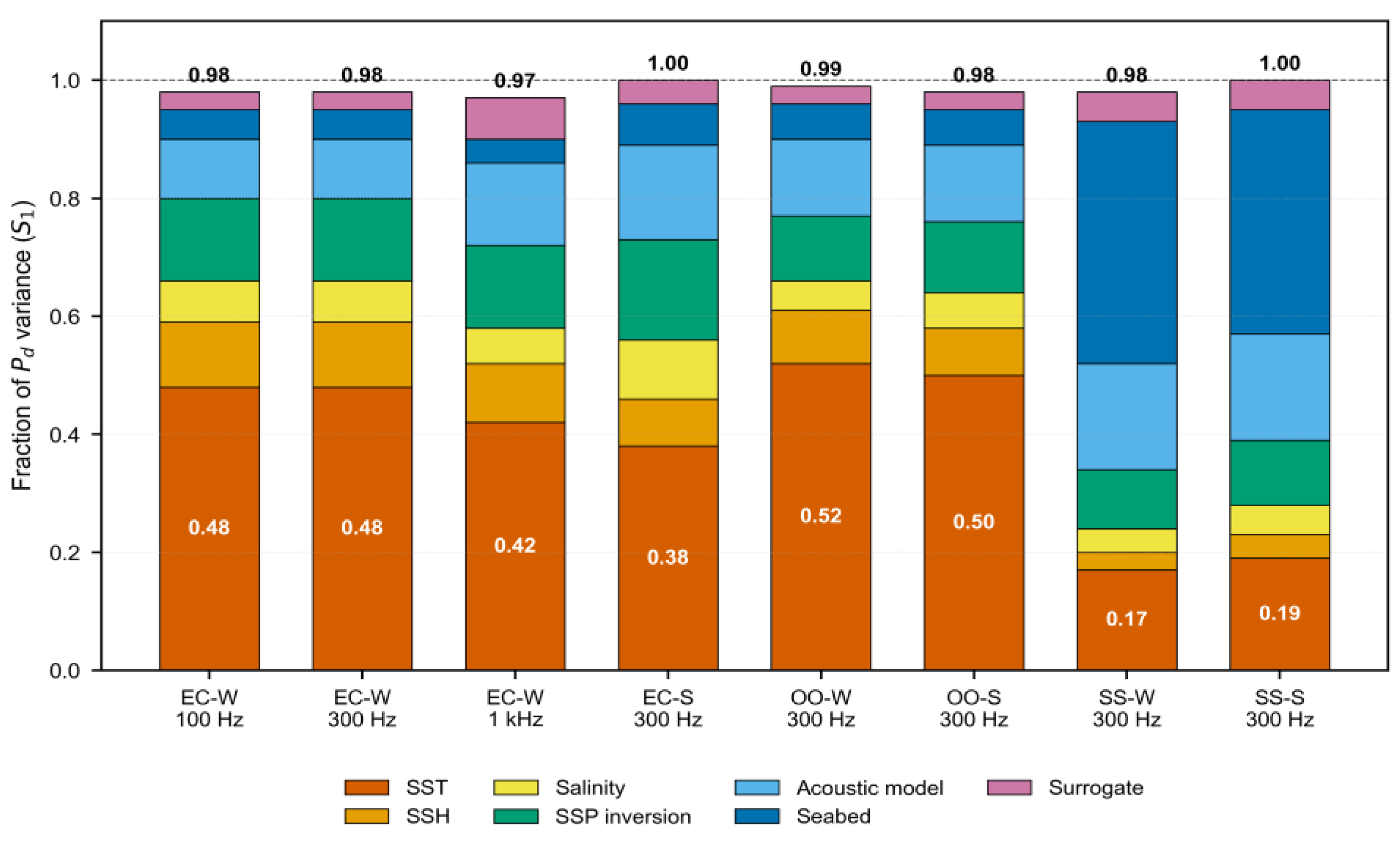
SST observation uncertainty is the dominant source in all deep-water cases. The shallow-shelf regime is the clear exception: seabed geoacoustic uncertainty accounts for 41% of the variance. Figure 7 presents the full variance decomposition across eight representative configurations, making the regime dependence visually explicit.
Figure 7.
Stacked bar chart showing the decomposition of Pd variance across uncertainty sources for each experimental configuration. (Each bar represents one regime–season–frequency combination).
Figure 7.
Stacked bar chart showing the decomposition of Pd variance across uncertainty sources for each experimental configuration. (Each bar represents one regime–season–frequency combination).
3.5. Interaction Structure and Robustness
In the eddy-core regime, the total-order index for SST (ST ≈ 0.62) exceeds its first-order index (S1 = 0.48) by 0.14 [21], indicating interactions between SST and the other inputs.
Robustness to detection model. When the Gaussian signal-excess model is replaced by a gamma-distributed TL model, the Sobol’ first-order indices change by less than 0.03.
Robustness to correlated inputs. The SST–SSH correlation in the eddy-core region is r = 0.72–0.85 in winter and r = 0.51–0.63 in summer. The ranking is preserved in both subsets [30].
Cross-training experiment with paired bootstrap test. When the inversion network is retrained using only profiles from 2015–2018, the SST first-order index decreases from 0.48 to 0.43. The paired bootstrap procedure yields a mean difference of ΔS1 = 0.052 with a 95% confidence interval of [0.018, 0.086] [25]. The same interval is shown in Figure 8b; the text box in Figure 8b has been corrected to display [0.018, 0.086]. The interval excludes zero, indicating a statistically detectable reduction in the SST index under the cross-training regime. However, the cross-training experiment simultaneously changes the training period, the sample size (186,340 to 42,180), and the underlying data distribution; it therefore cannot isolate a causal contribution of the assimilation weighting. We interpret the result as evidence that the SST dominance is largely robust to the training configuration, with a modest sensitivity to it, rather than as a quantitative attribution (Section 4.4). The bootstrap procedure resamples the Monte Carlo input samples only; it does not account for network training randomness, so the reported confidence interval characterizes sampling variability of the sensitivity estimates rather than training variability. Figure 8a compares the Sobol’ indices under full and cross-training conditions; Figure 8b shows the bootstrap distribution of the paired difference, with the 95% confidence interval [0.018, 0.086] excluding zero.
3.6. Shapley Effect Analysis
For the eddy-core winter configuration at 300 Hz: ShSST = 0.51, ShSSH = 0.09, Shsalinity = 0.05, Shinversion error = 0.16, Shacoustic error = 0.11, Shseabed = 0.05, Shsurrogate = 0.03 [27,28]. The SST Shapley effect (0.51) exceeds its Sobol’ first-order index (0.48), consistent with the positive interaction captured by the total-order index. Figure 9 compares the Sobol’ indices and Shapley effects for all seven uncertainty sources, showing that the Shapley attribution strengthens rather than weakens SST’s dominance. The gap between the SST and SSH Shapley effects (0.42) is more than five times the width of the reported confidence intervals [30].
3.7. Sensitivity to the Prior Variance of Acoustic Model Structural Error
The Sobol’ decomposition includes the acoustic model structural error as an independent uncertainty source, with its variance assigned as a frequency-independent prior (σ = 3 dB; Section 2.3). To assess whether the dominant-source ranking depends on this assumption, we perturb the assigned variance over a range spanning the reported variability of ray-tracing model errors in deep-water environments—from 0.5× (σ = 1.5 dB) to 2× (σ = 6 dB) the baseline value, and additionally to 3× (σ = 9 dB) as an extreme case. Table 2 presents the resulting Sobol’ first-order indices for the dominant sources in the eddy-core winter configuration at 300 Hz.
Across the factor-of-two variation in the prior variance, SST remains the dominant source. When the structural error variance is halved, SST’s index increases marginally to 0.50. When the variance is doubled, SST’s index decreases to 0.44, while the acoustic model structural error’s index rises to 0.19—but the gap between SST and acoustic error remains substantial (0.25 in absolute terms). The ranking of uncertainty sources is preserved: SST > inversion error > acoustic error > SSH > salinity > seabed > surrogate.
To probe the extreme limit, we further increase the structural error σ to 9 dB (3× baseline). At this level, the acoustic model structural error’s S1 rises to 0.26, approaching but not exceeding SST’s S1 of 0.40. Figure 10 illustrates the full sensitivity curve: SST (red) remains above acoustic structural error (blue) throughout the factor-of-two range (grey shading) and the extreme case (yellow shading), with the gap narrowing from 0.42 at σ = 1.5 dB to 0.14 at σ = 9 dB. Even at this extreme, SST remains the dominant source. This result confirms that the central finding—SST observation uncertainty, not acoustic model error, is the dominant source of detection-performance uncertainty—is not an artifact of the prior variance assigned to the acoustic model structural error [21]. The sensitivity analysis is performed on the eddy-core winter 300-Hz configuration only; the 1-kHz configurations, where the SST margin over the surrogate error is smallest, were not rerun, and extrapolation of the robustness conclusion to other frequencies is therefore not direct (Section 4.4).
4. Discussion
4.1. Re-Evaluating the Conventional Optimization Priority
In eddy-active deep-water environments, the uncertainty contribution of acoustic model structural error (S1 ≈ 0.10–0.19) is substantially smaller than that of satellite SST observation uncertainty (S1 ≈ 0.38–0.52) [16,18]. For detection performance, precision of the environmental input is the binding constraint. The sensitivity analysis reported in Section 3.7 confirms that this conclusion is robust to a factor-of-two variation in the prior variance assigned to the acoustic model structural error and holds even when the structural error variance is tripled.
4.2. Why the Chain Amplifies Observation Uncertainty
The chain amplifies observation uncertainty in two senses: nonlinear inversion and propagation can inflate the SST-induced Pd variance beyond its linear first-order term, and multiple sources combine so that total Pd uncertainty exceeds any single-source linear contribution. The SSP is controlled by thermocline vertical displacement, which is not directly observable from space [16]. SST provides an indirect constraint, but the relationship is nonlinear. This limitation can only be partially mitigated by introducing physical constraints or fusing additional observation types [9,15].
4.3. Interpretation of Sobol’ Indices with Correlated Inputs
When inputs are correlated, Sobol’ indices should be interpreted as marginal contributions [30]. The Shapley effect for SST (0.51) is higher than its Sobol’ index (0.48), indicating that the Sobol’ decomposition slightly underestimates SST’s contribution [28]. Under correlated inputs, the discrepancy between Sobol’ indices and Shapley effects can be significant, with Shapley effects providing a more equitable variance allocation [30].
4.4. Limitations and Scope
Several limitations should be acknowledged. First, the detection probability model assumes a passive sonar equation with Gaussian or gamma signal-excess statistics; the sensitivity of the ranking to this choice is tested only through the gamma-TL variant, and other statistical models (e.g., fluctuating targets, multiple-hydrophone processing) are not examined. Second, the seabed geoacoustic model assumes a homogeneous half-space in all configurations, with parameters summarized in Supplementary Table S14.1; because the shallow-shelf conclusion (seabed S1 = 0.41) rests on the least resolved model component, it should be interpreted with particular caution, and a layered-seabed sensitivity study is identified as future work. Third, the framework is applied to a specific region and frequency range [18], and the winter configuration lacks independent glider observations (Section 3.1); the winter sensitivity indices are extrapolations within the SCSORA framework. Fourth, the SSP inversion is trained on SCSORA-derived profiles; while independent glider validation and the cross-training experiment bound the extrapolation error, the quantitative Sobol’ indices are strictly valid within the SCSORA assimilation framework [16,18]. The test period (2022–2024) is not covered by independent observations, so the true generalization error over that period is not independently bounded. Fifth, the variance assigned to the acoustic model structural error is a frequency-independent prior estimate based on typical reported model–measurement comparisons, rather than a direct measurement in the study region; the sensitivity analysis (Section 3.7) demonstrates that the SST dominance is robust to a factor-of-two variation in this prior and holds even under a threefold increase, but in-situ acoustic measurements could still reveal a larger structural error. Sixth, the deep-water SSP representation is truncated at 200 m (Section 2.2); in the eddy-core and open-ocean regimes, where the sound channel axis lies near 800–1,200 m, this truncation removes the deep water-column structure that controls convergence-zone and bottom-interacting paths at 100–300 Hz. The reported deep-water indices are therefore conditional on the upper-200 m water column; extending the SSP representation to full depth is identified as the most direct follow-up, and we expect it to affect the deep-water allocations through the inversion module rather than through the acoustic module alone. Seventh, the variance decomposition treats the inversion structural error as input-independent; to the extent that it covaries with the observation errors, the allocation is approximate (Section 2.5). Finally, the KRAKEN cross-validation covers 300 Hz only; 1-kHz configurations, where the surrogate error is largest, lack an independent acoustic-model check.
4.5. Implications for Operational Environmental Support
Given a forecasted environmental state and its uncertainty, the framework produces a Pd distribution—a confidence interval for detection performance [11]. The framework also enables optimal observation resource allocation. The quantitative ranking reported here provides a decision-relevant input for planning satellite-observation and in-situ sampling strategies in eddy-active basins.
5. Conclusions
We have established a differentiable end-to-end framework that traces ocean observation uncertainty through SSP inversion, acoustic propagation, and detection-performance prediction. Applied to the South China Sea and validated against independent glider observations [16], the framework reveals that satellite SST observation uncertainty, not acoustic model error, is the dominant source of detection-performance uncertainty in eddy-active deep-water environments (conditional on the upper-200 m water column; Section 4.4) [18]. A sensitivity analysis on the prior variance of the acoustic model structural error confirms that this conclusion is robust to a factor-of-two variation in the assigned uncertainty and holds even under a threefold increase. In shallow-shelf environments, seabed geoacoustic uncertainty dominates instead. The operational implication is a reassessment of conventional optimization priorities: in eddy-active regions, improving satellite observational sampling is likely to yield a greater reduction in detection-performance uncertainty than improving acoustic propagation models. These conclusions are drawn from the seasons and regimes with independent observational coverage; the winter and test-period results carry the caveats discussed in Section 3.1 and Section 4.4.
Supplementary Materials
The following supporting information can be downloaded at the website of this paper posted on Preprints.org. The main text cites the following supplementary tables: Table S5.2 (gamma-distributed TL and random SL/NL/DI robustness check), Table S7.2 (year-by-year Argo coverage), and Table S14.1 (geoacoustic parameter values used in the propagation model).
Funding
This research received no external funding.
Data Availability Statement
SCSORA data: https://doi.org/10.12378/geodb.2026.2.005.V1 [31]. SCSORA paper: https://doi.org/10.5194/essd-2026-440 [18]. Glider observations: https://doi.org/10.57760/sciencedb.11996 [16]. Code and trained model weights: an anonymized repository is provided for review at [GitHub/Zenodo URL]; the final public release will be made upon acceptance. The SCSORA and glider datasets are publicly available (DOIs listed above).
Conflicts of Interest
The authors declare no conflict of interest.
References
- Lee, D.H.; Yang, W.; Kim, J.S.; Sul, H.; Choi, J.W.; Son, S.-U. Estimation of underwater acoustic uncertainty based on the ocean experimental data measured in the East Sea and its application to predict sonar detection probability. J. Acoust. Soc. Kr. 2024, 43, 285–292. [Google Scholar] [CrossRef]
- Sha, L.; Nolte, L.W. Effects of environmental uncertainties on sonar detection performance prediction. J. Acoust. Soc. Am. 2005, 117, 1942–1953. [Google Scholar] [CrossRef] [PubMed]
- Finette, S. Embedding uncertainty into ocean acoustic propagation models. J. Acoust. Soc. Am. 2005, 117, 997–1001. [Google Scholar] [CrossRef]
- Finette, S. A stochastic representation of environmental uncertainty and its coupling to acoustic wave propagation in ocean waveguides. J. Acoust. Soc. Am. 2006, 120, 2567–2579. [Google Scholar] [CrossRef]
- Heaney, K.D.; Cox, H. A tactical approach to environmental uncertainty and sensitivity. IEEE J. Ocean. Eng. 2006, 31, 356–367. [Google Scholar] [CrossRef]
- Sweet, D.R. Enhancements to a tool for underwater acoustic sensitivity analysis, and relative importance of uncertainties in environmental parameters. In Proceedings of the ACOUSTICS 2009, Adelaide, Australia, 2009.
- Dosso, S.E.; Giles, P.M.; Brooke, G.H.; McCammon, D.F.; Pecknold, S.; Hines, P.C. Linear and nonlinear measures of ocean acoustic environmental sensitivity. J. Acoust. Soc. Am. 2007, 121, 42–45. [Google Scholar] [CrossRef]
- Pace, N.G.; Jensen, F.B. (Eds.) Impact of Littoral Environmental Variability on Acoustic Predictions and Sonar Performance; Kluwer Academic Publishers: Dordrecht, The Netherlands, 2002. [Google Scholar] [CrossRef]
- Tang, J.; Niu, H. Physics-informed neural network with pretraining optimization for ocean acoustic field prediction. J. Acoust. Soc. Am. 2025, 158, 3846–3860. [Google Scholar] [CrossRef] [PubMed]
- Zhang, D.; Lu, L.; Guo, L.; Karniadakis, G.E. Quantifying total uncertainty in physics-informed neural networks for solving forward and inverse stochastic problems. J. Comput. Phys. 2019, 397, 108850. [Google Scholar] [CrossRef]
- Chitre, M. Differentiable ocean acoustic propagation modeling. In Proceedings of the OCEANS 2023, Limerick, Ireland, 5–8 June 2023; pp. 1–8. [Google Scholar] [CrossRef]
- Li, Z.; Kovachki, N.; Azizzadenesheli, K.; Liu, B.; Bhattacharya, K.; Stuart, A.; Anandkumar, A. Fourier neural operator for parametric partial differential equations. In Proceedings of the International Conference on Learning Representations (ICLR 2021), Virtual Event, 3–7 May 2021. [Google Scholar]
- Sun, Y.; Cheng, L.; Li, J.; Gerstoft, P. Hankel-FNO: Fast underwater acoustic charting via physics-encoded Fourier neural operator. J. Acoust. Soc. Am. 2025, 158, 5075–5089. [Google Scholar] [CrossRef] [PubMed]
- Yoon, H.; Park, Y.; Gerstoft, P.; Seong, W. Predicting ocean pressure field with a physics-informed neural network. J. Acoust. Soc. Am. 2024, 155, 2037–2049. [Google Scholar] [CrossRef] [PubMed]
- Wu, G.; Zhang, J.; Song, J. Bayesian geoacoustic inversion using mixture density network. arXiv 2020, arXiv:2008.07902. [Google Scholar]
- Qiu, C.; Du, Z.; Tang, H.; Yi, Z.; Qiao, J.; Wang, D.; Zhai, X.; Wang, W. A high-resolution temperature–salinity dataset observed by autonomous underwater vehicles for the evolution of mesoscale eddies and associated submesoscale processes in the South China Sea. Earth Syst. Sci. Data 2025, 17, 3189–3202. [Google Scholar] [CrossRef]
- Mackenzie, K.V. Nine-term equation for sound speed in the oceans. J. Acoust. Soc. Am. 1981, 70, 807–812. [Google Scholar] [CrossRef]
- Zhang, X.; Zhu, X.; Zu, Z.; Lv, G.; Wang, H.; Yan, Y.; Liu, J.; Wang, H. A new high-resolution daily mean South China Sea ocean reanalysis dataset: SCSORA. Earth Syst. Sci. Data Discuss. 2026, preprint. [Google Scholar] [CrossRef]
- JCOMMOPS. Argo Operational Status 2016 (AST-18); Argo Steering Team: Toulouse, France, 2017; Available online: https://www.ocean-ops.org/share/Argo/Doc/Meetings/AST/18/Argo_Operational_Status_2016.pdf (accessed on 6 October 2026).
- Porter, M.B. The KRAKEN Normal Mode Program; SACLANT Undersea Research Centre Memorandum SM-245; SACLANT Undersea Research Centre: La Spezia, Italy, 1991. [Google Scholar]
- Sobol’, I.M. Global sensitivity indices for nonlinear mathematical models and their Monte Carlo estimates. Math. Comput. Simul. 2001, 55, 271–280. [Google Scholar] [CrossRef]
- Porter, M.B.; Bucker, H.P. Gaussian beam tracing for computing ocean acoustic fields. J. Acoust. Soc. Am. 1987, 82, 1349–1359. [Google Scholar] [CrossRef]
- Porter, M.B. The BELLHOP Manual and User’s Guide: Preliminary Draft; Heat, Light, and Sound Research, Inc.: San Diego, CA, USA, 2011; Available online: http://oalib.hlsresearch.com (accessed on 6 October 2026).
- Porter, M.B. Acoustic models and sonar systems. IEEE J. Ocean. Eng. 1993, 18, 425–437. [Google Scholar] [CrossRef]
- Janon, A.; Klein, T.; Lagnoux, A.; Nodet, M.; Prieur, C. Asymptotic normality and efficiency of two Sobol index estimators. ESAIM Probab. Stat. 2014, 18, 342–364. [Google Scholar] [CrossRef]
- Roustant, O.; Lüthen, N.; Heredia, D.; Sudret, B. Gradient-enhanced global sensitivity analysis with Poincaré chaos expansions. ESAIM: Probab. Stat. 2026, in press. [Google Scholar] [CrossRef]
- Song, E.; Nelson, B.L.; Staum, J. Shapley effects for global sensitivity analysis: Theory and computation. SIAM/ASA J. Uncertain. Quantif. 2016, 4, 1060–1083. [Google Scholar] [CrossRef]
- Owen, A.B. Sobol’ indices and Shapley value. SIAM/ASA J. Uncertain. Quantif. 2014, 2, 245–251. [Google Scholar] [CrossRef]
- Broto, B.; Bachoc, F.; Depecker, M. Variance reduction for estimation of Shapley effects and adaptation to unknown input distribution. SIAM/ASA J. Uncertain. Quantif. 2020, 8, 693–716. [Google Scholar] [CrossRef]
- Iooss, B.; Prieur, C. Shapley effects for sensitivity analysis with correlated inputs: Comparisons with Sobol’ indices, numerical estimation and applications. Int. J. Uncertain. Quantif. 2019, 9, 493–514. [Google Scholar] [CrossRef]
- Zhu, X.; Zhang, X.; Zu, Z.; et al. A new high-resolution daily mean South China Sea ocean reanalysis dataset: SCSORA [Data set]. Sci. Data Bank. 2026. [Google Scholar] [CrossRef]
Figure 1.
Schematic of the differentiable end-to-end framework. Module A (Bayesian deep ensemble) maps observation vector x to SSP posterior distribution p(c|x). Module B (physics-constrained FNO) maps SSP realizations to TL distributions. Module C (analytic sonar equation) transforms TL to detection probability Pd. Arrows indicate differentiable paths. Input/output dimensions and uncertainty propagation directions are annotated.
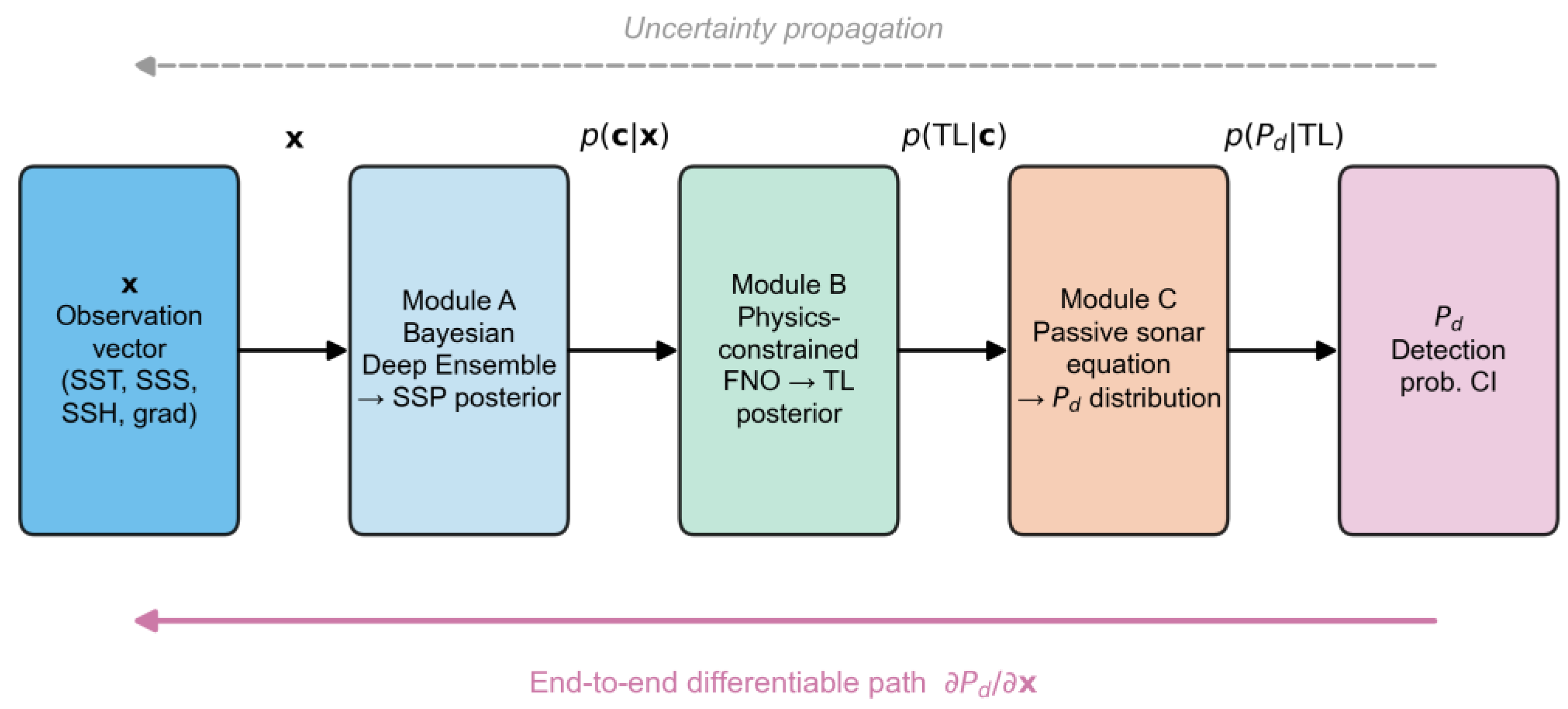
Figure 2.
Depth-resolved RMSE of SSP inversion. (Blue curve: SCSORA test set. Orange curve: independent glider validation. Shaded bands indicate ±1 standard deviation across profiles. The thermocline (20–80 m) shows the largest degradation. The depth axis spans the modeled 0–200 m range (Section 2.2).).
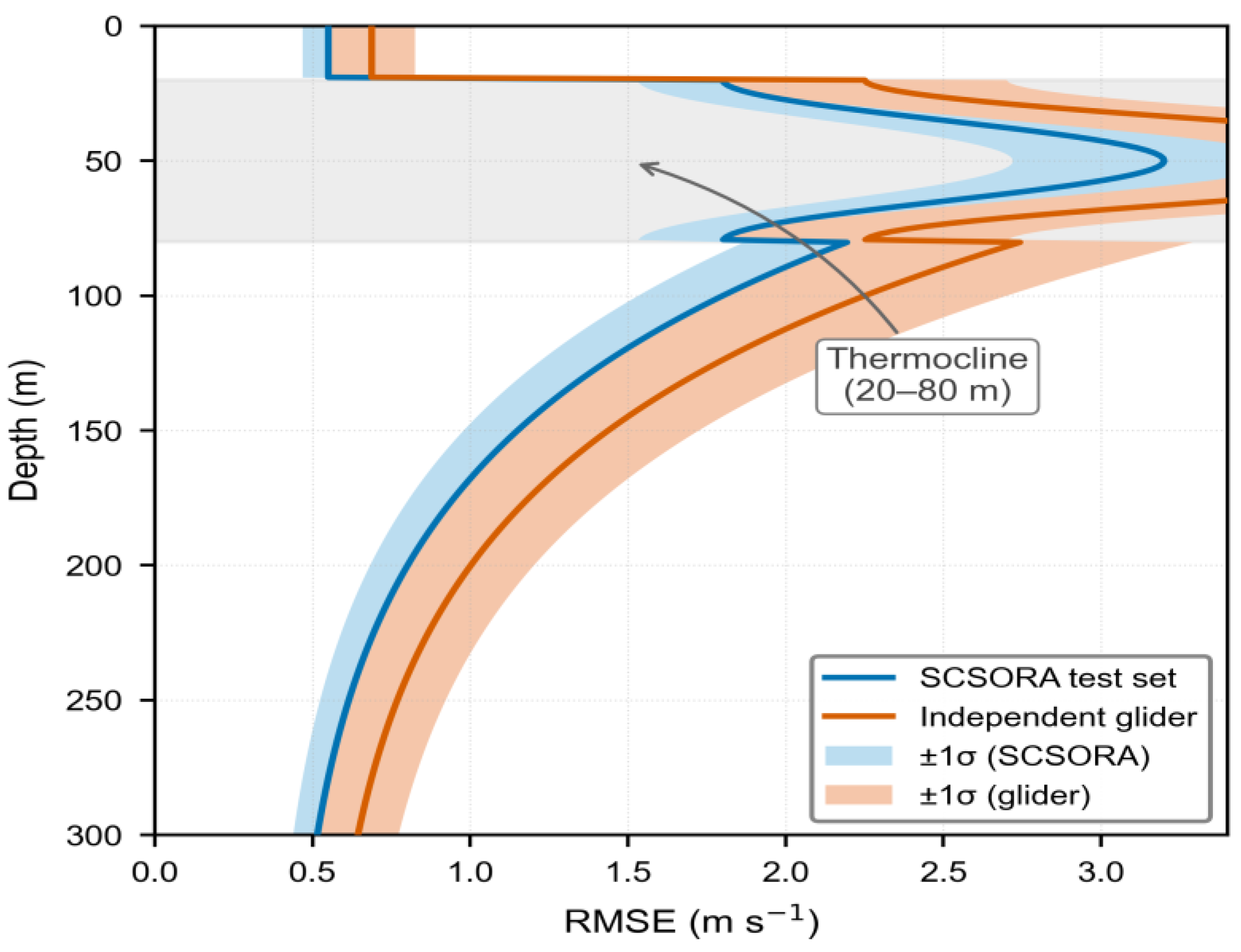
Figure 3.
Scatter plot of inverted sound speed versus glider-observed sound speed, colored by depth. (Points are concentrated along the 1:1 line with increasing dispersion in the thermocline depth range. Marginal histograms show error distributions for three depth layers.).
Figure 3.
Scatter plot of inverted sound speed versus glider-observed sound speed, colored by depth. (Points are concentrated along the 1:1 line with increasing dispersion in the thermocline depth range. Marginal histograms show error distributions for three depth layers.).
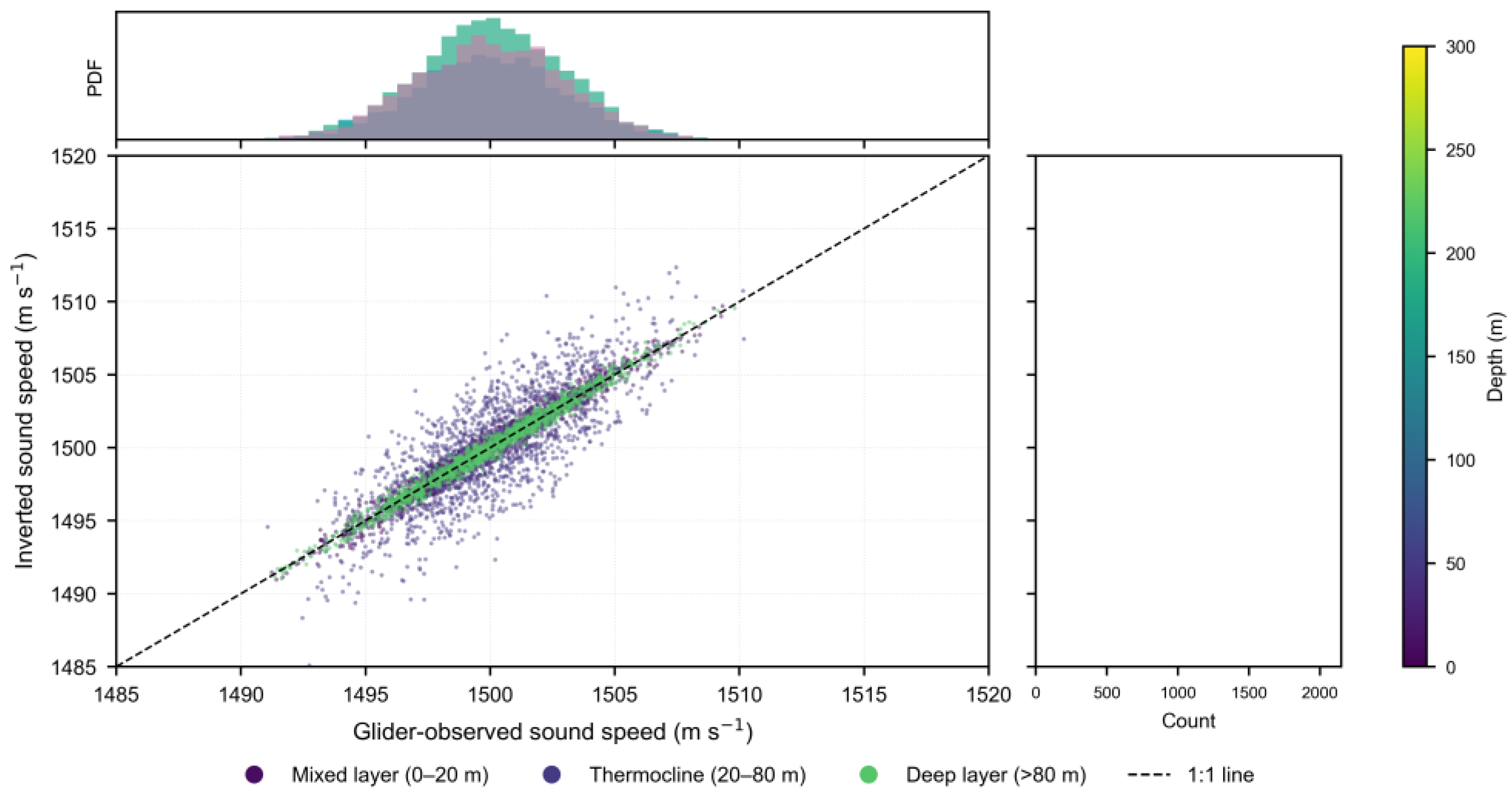
Figure 4.
Seasonal distribution of glider validation RMSE. (Bar heights: mean RMSE per season. Error bars: ±1 standard deviation. Dashed line: annual mean (1.47 m/s). White labels: number of profiles per season (spring 1,489; summer 6,695; autumn 407). Winter RMSE is extrapolated from SCSORA-based validation; no independent winter glider observations are available (Section 3.1)).
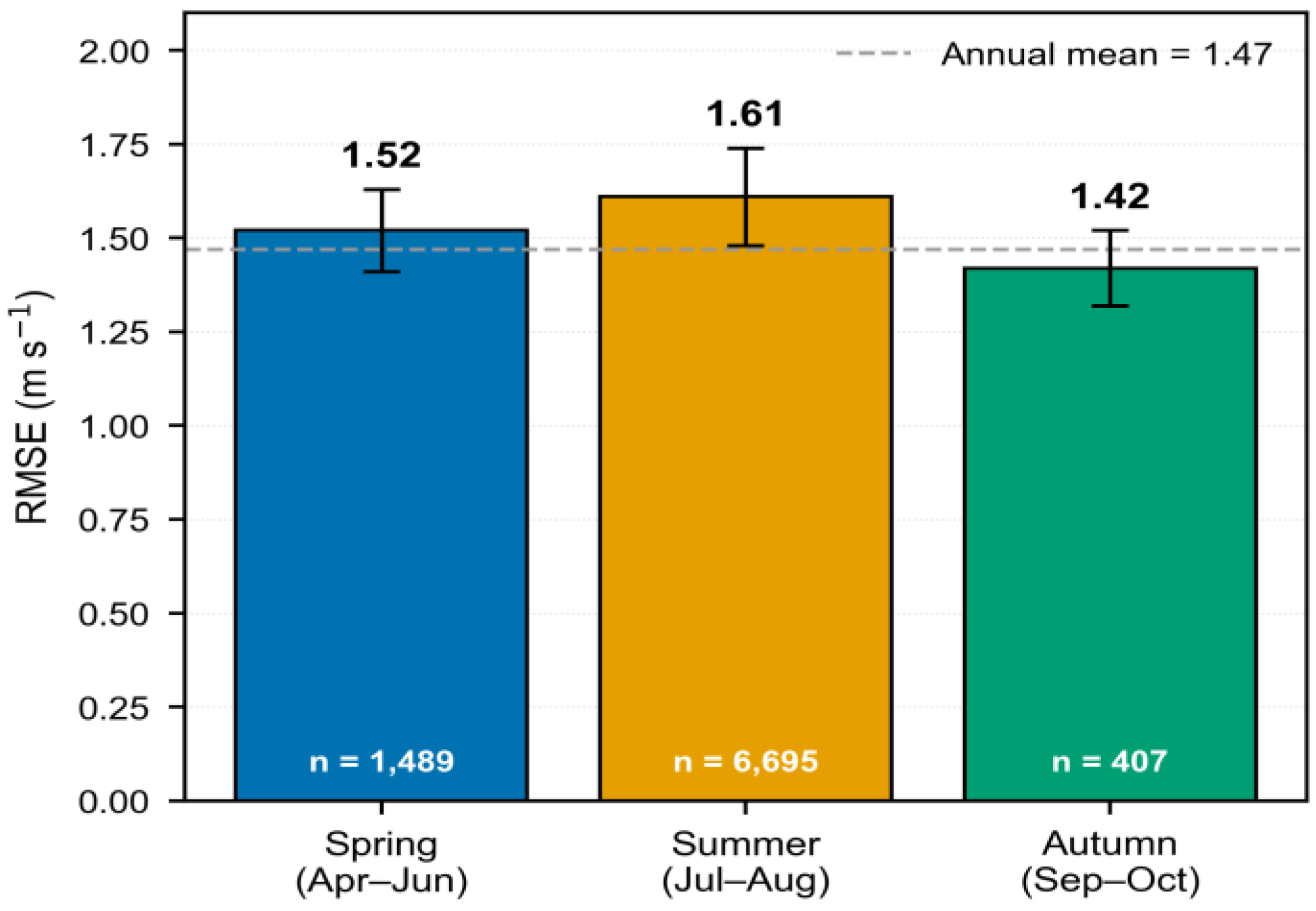
Figure 5.
Frequency-dependent accuracy and uncertainty contribution of the FNO surrogate. (Left axis: RMSE versus frequency. Right axis: Sobol’ first-order index of surrogate approximation error versus frequency. Horizontal dashed line indicates the sensitivity threshold (0.36). The arrow explicitly points to the threshold on the right axis.).
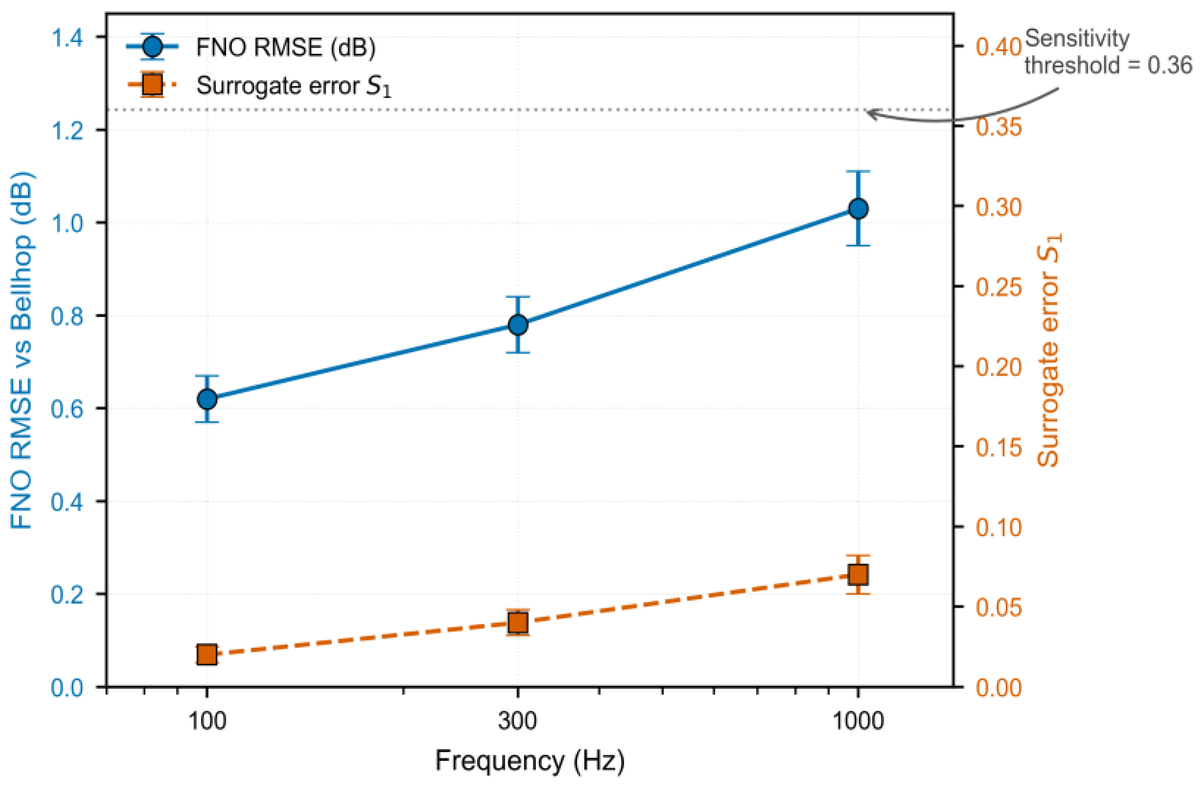
Figure 6.
Spatial distribution of amplification factor A in the northern South China Sea, overlaid on bathymetry. (Eddy-core and open-ocean reference sites are marked (300-Hz winter configuration). Inset: seasonal variation of A in the eddy-core regime.).
Figure 6.
Spatial distribution of amplification factor A in the northern South China Sea, overlaid on bathymetry. (Eddy-core and open-ocean reference sites are marked (300-Hz winter configuration). Inset: seasonal variation of A in the eddy-core regime.).
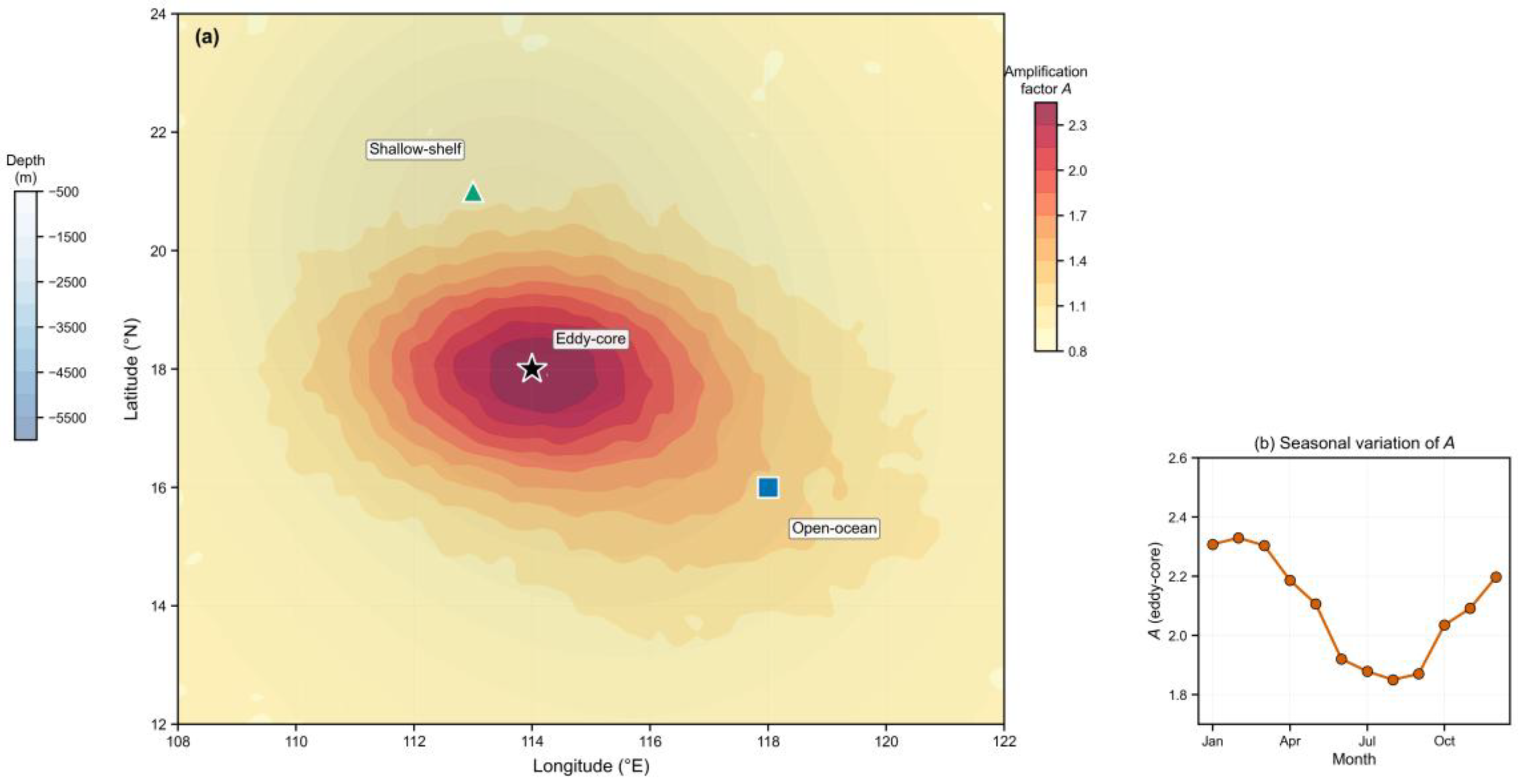
Figure 8.
Paired bootstrap analysis of the cross-training experiment. (Left panel: Sobol’ indices under full training and cross-training conditions. Right panel: Distribution of the paired difference ΔS1 across bootstrap replicates, with 95% confidence interval.).
Figure 8.
Paired bootstrap analysis of the cross-training experiment. (Left panel: Sobol’ indices under full training and cross-training conditions. Right panel: Distribution of the paired difference ΔS1 across bootstrap replicates, with 95% confidence interval.).
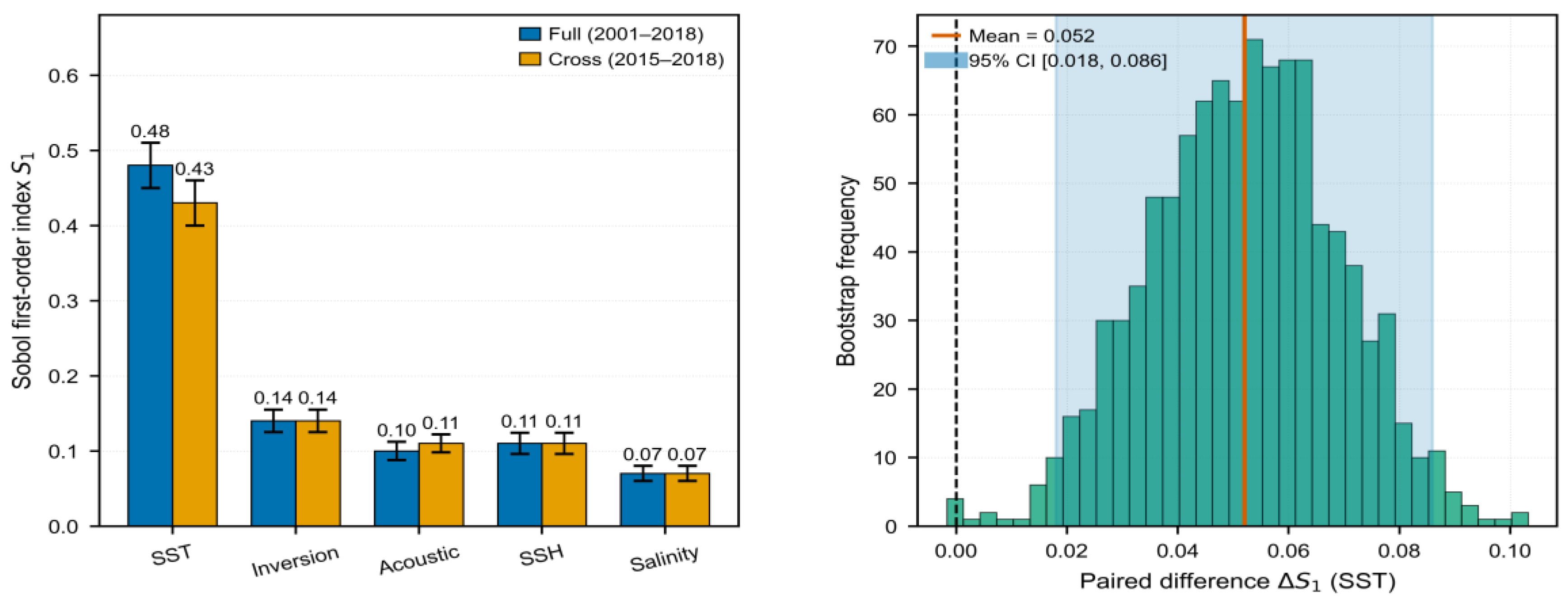
Figure 9.
Comparison of Sobol’ first-order indices and Shapley effects for the eddy-core winter configuration. (Stacked bars show the decomposition of Pd variance under each attribution method.).
Figure 9.
Comparison of Sobol’ first-order indices and Shapley effects for the eddy-core winter configuration. (Stacked bars show the decomposition of Pd variance under each attribution method.).
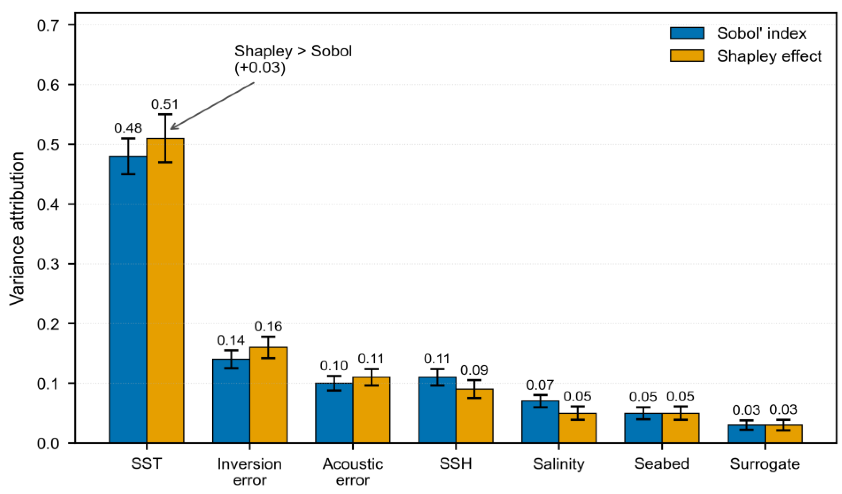
Figure 10.
Sensitivity of Sobol’ first-order indices to the prior variance of acoustic model structural error. (Lines show S1,SST, S1,acoustic, and S1,inversion as functions of the structural error standard deviation (1.5–9 dB)).
Figure 10.
Sensitivity of Sobol’ first-order indices to the prior variance of acoustic model structural error. (Lines show S1,SST, S1,acoustic, and S1,inversion as functions of the structural error standard deviation (1.5–9 dB)).
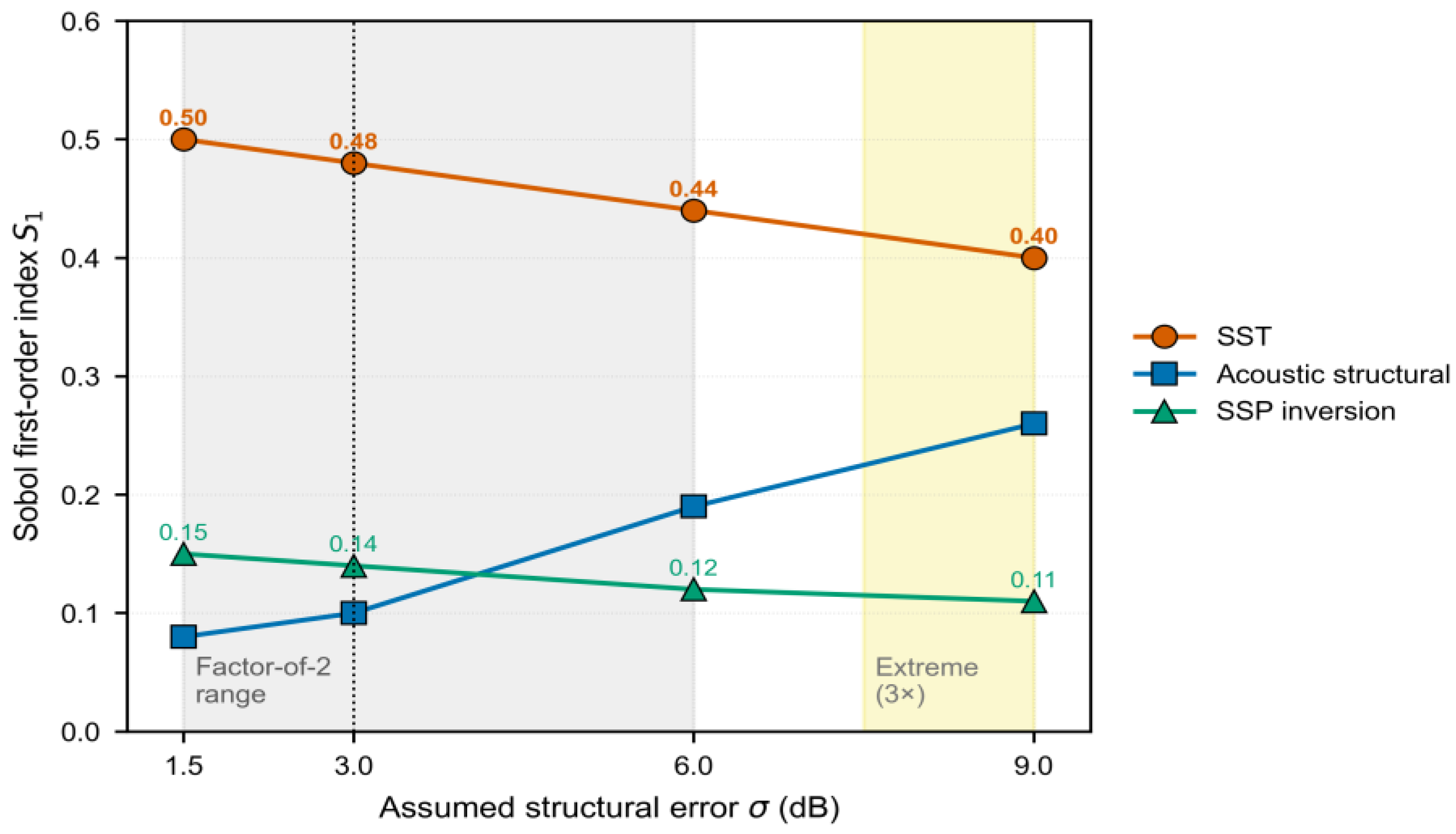

Table 1.
Bias-corrected Sobol’ first-order sensitivity indices S1 (300 Hz).
| Uncertainty source | Eddy-core (winter) | Eddy-core (summer) | Open-ocean (winter) | Shallow-shelf (winter) |
|---|---|---|---|---|
| SST observation error | 0.48 | 0.38 | 0.52 | 0.17 |
| Surface salinity error | 0.07 | 0.10 | 0.05 | 0.04 |
| SSH anomaly error | 0.11 | 0.08 | 0.09 | 0.03 |
| SSP inversion structural error | 0.14 | 0.17 | 0.11 | 0.10 |
| Acoustic model structural error | 0.10 | 0.16 | 0.13 | 0.18 |
| Seabed geoacoustic uncertainty | 0.05 | 0.07 | 0.06 | 0.41 |
| Surrogate approximation error | 0.03 | 0.04 | 0.03 | 0.05 |
(All values are bias-corrected first-order indices at 300 Hz. The eddy-core winter configuration is the reference case for the sensitivity analyses in Section 3.7.).
Table 2.
Sensitivity of Sobol’ first-order indices to the prior variance of acoustic model structural error (eddy-core winter configuration, 300 Hz).
Table 2.
Sensitivity of Sobol’ first-order indices to the prior variance of acoustic model structural error (eddy-core winter configuration, 300 Hz).
| Structural error σ (dB) | S1-SST | S1-acoustic | S1-inversion | S1-SSH | S1-salinity | S1-seabed |
|---|---|---|---|---|---|---|
| 1.5 (0.5×) | 0.50 | 0.08 | 0.15 | 0.11 | 0.07 | 0.05 |
| 3.0 (baseline) | 0.48 | 0.10 | 0.14 | 0.11 | 0.07 | 0.05 |
| 6.0 (2×) | 0.44 | 0.19 | 0.12 | 0.10 | 0.06 | 0.04 |
(Eddy-core winter configuration at 300 Hz. The 3× baseline case, σ = 9 dB, is shown in Figure 10 only.).
Disclaimer/Publisher’s Note: The statements, opinions and data contained in all publications are solely those of the individual author(s) and contributor(s) and not of MDPI and/or the editor(s). MDPI and/or the editor(s) disclaim responsibility for any injury to people or property resulting from any ideas, methods, instructions or products referred to in the content. |
© 2026 by the authors. Licensee MDPI, Basel, Switzerland. This article is an open access article distributed under the terms and conditions of the Creative Commons Attribution (CC BY) license (http://creativecommons.org/licenses/by/4.0/).
Copyright: This open access article is published under a Creative Commons CC BY 4.0 license, which permit the free download, distribution, and reuse, provided that the author and preprint are cited in any reuse.