

Submitted:
24 September 2026
Posted:
12 October 2026
You are already at the latest version
Abstract
Electroencephalography (EEG) records cortical activity with high temporal resolution without radiation and at low cost, which makes it a practical signal for automated screening of neurological disorders. Deep learning classifies EEG with high accuracy, but most models distinguish only two conditions and give no account of their decisions, which limits their use in screening and decision support. This paper presents SpectraXAI, an interpretable frequency-aware deep learning model that assigns resting-state EEG to four diagnostic categories: Alzheimer’s disease, Parkinson’s disease, schizophrenia, and healthy control. The model filters each EEG window into the delta, theta, alpha, beta, and gamma bands and processes every band in a separate convolutional branch with squeeze-and-excitation recalibration. Softmax-weighted band attention and temporal attention then combine the spectral and temporal evidence, and the same attention weights are intrinsic explanations of each prediction. Under a subject-disjoint evaluation protocol that prevents window leakage, the model reached 94.43% accuracy, 96.74% balanced accuracy, and 93.82% macro-F1 on 20,760 windows from 173 unseen subjects while using only 0.10 million parameters. An ablation study confirmed that the attention modules account for most of the improvement over a plain convolutional baseline. Attention weights, feature-attention heatmaps, Grad-CAM, and t-SNE embeddings trace each decision to specific frequency bands, time segments, and learned features, therefore the frequency structure that drives the accuracy also makes the predictions inspectable.
Keywords:
explainable artificial intelligence
; deep learning
; EEG
; neurological disorders
; frequency-band decomposition
; attention mechanism
1. Introduction
Neurological and neuropsychiatric disorders such as Alzheimer’s disease (AD), Parkinson’s disease (PD), schizophrenia (SCZ), and epilepsy affect memory, movement, and cognition, and they progress if left untreated [1,2]. Early diagnosis matters because timely intervention slows decline and lowers the long-term clinical burden [3]. Standard workups combine clinical assessment, neuropsychological testing, and imaging such as MRI or PET. These tools are informative but slow, expensive, and poorly suited to repeated monitoring. Electroencephalography (EEG) offers a different trade-off. An EEG montage records cortical electrical activity as a multi-channel signal at millisecond resolution, without radiation and at a fraction of the cost of imaging [4]. Those properties make EEG a practical front end for automated screening and decision support.
EEG data exemplify the challenges that motivate advanced mathematical methods in biomedical machine learning: the signals are high-dimensional, noisy, heterogeneous across acquisition sites, and imbalanced across diagnostic groups. Deep learning removes much of the handcrafted feature engineering that older EEG pipelines relied on and learns discriminative patterns directly from the recordings [4]. Yet three issues keep recurring in the literature. First, most models target a single disorder or a binary task such as patient versus control [1,5,6,7], which limits clinical value when several disorders share overlapping EEG signatures. Second, strong accuracy is often reported on small or narrow cohorts and without subject-level validation, so generalization is uncertain [2,4,8]. Third, many high-performing models stay opaque, and clinicians resist predictions they cannot inspect [9,10].
This study addresses those gaps together. SpectraXAI classifies resting-state EEG into AD, healthy control (HC), PD, and SCZ. Rather than treating the recording as one raw sequence, it splits each window into the five canonical bands, delta through gamma, and gives each band its own convolutional branch. A squeeze-and-excitation block learns feature importance inside each branch, a band-attention module weights the five bands per prediction, and a temporal-attention module selects the informative time segments before the classifier. The design is predictive and interpretable at the same time, since band attention, temporal attention, feature-attention heatmaps, Grad-CAM, and embedding visualization reveal which frequencies, time regions, and features support each decision. In this way, the mathematical structure of the model, band-wise decomposition followed by softmax-weighted attention mappings, is also the source of its transparency, which is the kind of principled coupling between model design and interpretability that machine learning for biomedical applications requires.
The contributions are as follows:
- A four-class EEG framework that distinguishes AD, HC, PD, and SCZ from a single harmonized dataset.
- A frequency-aware architecture in which delta, theta, alpha, beta, and gamma bands are processed by separate convolutional branches with squeeze-and-excitation recalibration.
- Band attention and temporal attention that fuse spectral and temporal evidence and, at the same time, expose it for inspection.
- A subject-level evaluation protocol that removes window leakage and reports performance on unseen subjects, with a statistical analysis of the results and an ablation against a convolutional baseline.
- A compact model of about 0.10 million parameters, which is small enough to be attractive for edge and point-of-care deployment.
The remainder of the paper is organized as follows. Section 2 reviews related work. Section 3 describes the data, preprocessing, architecture, implementation, and explainability pipeline. Section 4 reports classification performance, the ablation, the statistical analysis, and the interpretability outputs. Section 5 positions the results against related work and states the limitations, and Section 6 concludes.
2. Related Work
2.1. Deep Learning Architectures for EEG
Convolutional networks are the most common backbone for EEG, since they learn local time-frequency patterns directly from the signal and remove the need for handcrafted features [4]. Later work added mechanisms that model longer-range and cross-band structure. Squeeze-and-excitation and spectral fusion improved motor-imagery decoding by recalibrating feature channels and combining sub-band representations [11], and geometric formulations on the covariance manifold pushed accuracy further [12]. Graph networks capture the spatial layout of electrodes, either as local-global-graph representations [13] or as sparse spectral graphs for epileptic signals [8]. Multitask and clustering-based feature learning [14] and spatio-spectral convolutional representations [15] show that separating spatial, spectral, and temporal factors helps generalization. Learnable band-pass front ends make the spectral factor explicit inside the network [16]. SpectraXAI follows this line by giving each frequency band its own branch, which keeps the spectral factor explicit rather than entangled inside a single convolutional stack.
2.2. Attention and Transformers for EEG
Attention has become central to EEG modeling because it can weight the parts of a signal that matter and, as a by-product, expose those weights for inspection. Time-distributed attention isolates informative segments within a limb-specific task [17,18], and dual-scale fusion combines fine and coarse temporal views [19]. Transformer hybrids such as the EEG Conformer join convolutional front ends with self-attention and add a class-activation visualization [20], while interactive-frequency and convolutional-transformer variants target the spectral axis directly [21,22]. Multi-scale vision transformers extend this to richer temporal hierarchies [23], and a transformer combining spatial and temporal information classifies raw EEG without heavy preprocessing [24]. Recent foundation models pre-train on large unlabeled EEG corpora and transfer to many downstream tasks, including LaBraM [25], EEGPT [26], and image-decoding transformers [27]. These models are powerful but data-hungry and hard to interpret, whereas SpectraXAI keeps a small, transparent attention design suited to modest clinical datasets.
2.3. Explainable AI in Biomedical Signals
Interpretability is a precondition for clinical adoption, so recent EEG studies pair predictions with explanations. Attention maps and SHAP values have been used for SCZ risk stratification [9], pairwise common spatial patterns with random forests give transparent dementia features [28,29], and graph-learning models expose the connectivity behind a PD diagnosis [10,30]. Sleep-staging networks add interpretability and uncertainty quantification on top of attention [31,32], and hemisphere-asymmetry and depression networks link learned features back to physiology [33,34]. SpectraXAI contributes intrinsic explanations at three levels, band, feature, and time, and adds a post-hoc Grad-CAM view, so a single prediction can be traced through the spectral and temporal evidence. Within this literature, the present work targets the multi-disorder screening problem that single-disease studies leave open.
3. Materials and Methods
The framework classifies neurological conditions from resting-state EEG using frequency-aware representation learning and attention-based explainability. Let the dataset be , where is the recording of subject i, is the number of channels after harmonization, T is the number of temporal samples, and labels AD, HC, PD, and SCZ. The goal is to learn a mapping that returns a posterior over the four classes.
3.1. Datasets
We built a combined open-source EEG dataset from three disease-specific cohorts so that the task becomes multi-class screening rather than repeated binary comparisons (Table 1). The PD recordings come from the resting-state dataset of Jackson et al. [35], which captures the altered synchronisation and spectral changes associated with the disorder. The AD and HC recordings come from the routine-EEG dementia dataset of Miltiadous et al. [36], where AD is linked to slowed activity, higher delta and theta power, and reduced fast activity. The SCZ recordings come from the resting-state dataset of Olejarczyk and Jernajczyk [37], which reflects abnormal oscillations, altered gamma activity, and disrupted functional integration. Using three cohorts lets the model learn neurodegenerative and neuropsychiatric patterns and tell them apart.
Because the cohorts differ in montage and protocol, we harmonized them before training. All recordings were mapped to a common 19-channel format; recordings with more channels were truncated and recordings with fewer were zero-padded. Signals were then aligned to the shortest shared duration and rescaled to a common amplitude range to reduce inter-dataset variability. The result is a single subject-level dataset used for windowing, band decomposition, and classification.
Because the diagnostic groups were obtained from independent public cohorts, diagnostic label and dataset of origin are partly associated. Differences in recording hardware, reference scheme, montage, acquisition protocol, recruitment criteria, and source-level preprocessing may therefore remain in the harmonized signals. Subject-level partitioning prevents windows from the same participant from appearing in more than one split, but it does not fully remove this source-related confounding. Healthy controls from the available cohorts were combined into a single HC class before subject-level partitioning; nevertheless, the disease groups remain linked to their respective source datasets. The present evaluation should therefore be interpreted as classification within a harmonized multicohort dataset rather than definitive evidence of acquisition-invariant disease recognition.
The harmonization procedure standardized channel count, sampling length, and amplitude scale so that recordings could be processed by one architecture. However, channel truncation may discard information, zero-padding may introduce artificial missing-channel patterns, and amplitude normalization cannot remove differences in amplifier response, electrode reference, or source-level filtering. These limitations were considered when interpreting the results, and no claim is made that harmonization completely eliminates inter-dataset variability.
3.2. Subject-Level Partitioning, Windowing, and Normalization
To prevent leakage, we split the data by subject rather than by window, so every window from a given subject stays within one of the training, validation, or test sets:
This evaluates the model on unseen subjects, which is the realistic clinical setting, instead of unseen windows from subjects already observed during training.
Each recording is segmented into fixed windows. With sampling frequency Hz and window length s, each window holds samples. For subject i, the k-th window is with stride and overlap . Every window is normalized per channel using z-scoring,
where and are the channel mean and standard deviation and is a small constant for numerical stability.
3.3. Frequency-Band Decomposition
EEG rhythms carry distinct physiological information, so each normalized window is band-pass filtered into the five canonical bands listed in Table 2. Writing for the band-pass operator of band b, the multi-band tensor is
with . Training windows are augmented on the fly with additive Gaussian noise, small temporal shifts, channel dropout, and band dropout. Augmentation is applied only during training, never at validation or test time.
3.4. Frequency-Aware SpectraXAI Architecture
The model has five band-specific convolutional branches, squeeze-and-excitation feature attention, band attention, temporal attention, and a classifier (Figure 1). Table 3 lists the layers of one band branch and the fusion stage.
Band-specific feature extraction. For band b, the input passes through two convolutional blocks with batch normalization, ELU activation, dropout, and max-pooling, followed by a projection to a fixed temporal resolution through adaptive average pooling. This yields , where is the number of learned feature channels and is the compressed temporal length.
Squeeze-and-excitation feature attention. To weight feature channels inside a branch, global temporal pooling produces , and a small gating network returns the attention vector
where is ReLU and is the sigmoid. This recalibrates each band by amplifying informative feature channels, following the temporal-spectral squeeze-and-excitation idea introduced for EEG decoding [11].
Band attention. The five recalibrated maps are scored and normalized, then fused into a single spectral representation:
where . The weights show which bands drove a given prediction.
Temporal attention. The fused map is scored along time to locate the informative segments, giving weights and an embedding :
where g is produced by a small temporal convolutional scorer.
Classification. A fully connected head maps the embedding to class logits o, and a softmax returns the posterior:
3.5. Training
The model is trained with label-smoothed cross-entropy. For a sample with true label y and smoothing factor , the smoothed target is with , and the per-sample loss is
Optimization uses AdamW with weight decay and gradient-norm clipping. Class imbalance is handled with a weighted sampler that draws each class with probability inversely proportional to its window count, so the minority SCZ class is not overwhelmed by the majority healthy class. Training runs for a fixed number of epochs, the learning rate is reduced when validation macro-F1 plateaus, and the checkpoint with the best validation macro-F1 is kept for testing. Algorithm 1 summarizes the pipeline.
| Algorithm 1 SpectraXAI training and explanation pipeline. |
| Require: EEG dataset , bands , epochs E, learning rate |
| Ensure: Best model , predictions , explanations |
|
3.6. Implementation Details
The framework was implemented in PyTorch and trained on a single GPU. Table 4 lists the settings, all fixed across runs for reproducibility, and a fixed random seed was used throughout. Table 5 reports the parameter budget. The full model has about 0.10 million trainable parameters, most of them in the five band branches and the band-attention scorer. The convolutional baseline used in the ablation is smaller still, which makes the comparison in Section 4 a comparison of design rather than of raw capacity. A model of this size is small enough to run on modest hardware, which matters for point-of-care deployment.
3.7. Explainability and Evaluation
Explanations come from both the learned attention weights and a post-hoc gradient map. Band attention and temporal attention are read directly from the network and averaged within a class to give class-level spectral and temporal relevance. The squeeze-and-excitation vectors provide feature-level relevance across bands and learned channels. For a local, prediction-specific view, Grad-CAM weights the activations of a convolutional layer by the gradient of the target logit, , and forms the normalized temporal relevance map .
Performance is reported at the window level with accuracy, balanced accuracy, macro-precision, macro-recall, and macro-F1. Balanced accuracy averages per-class recall and macro-F1 averages per-class F1, so both weight every class equally regardless of support, which matters because the test set is imbalanced, with HC the largest class and SCZ the smallest. All test windows belong to 173 participants who were completely unseen during training, so the evaluation is subject-disjoint, but the reported 94.43% accuracy remains a window-level metric rather than participant-level diagnostic accuracy. To quantify sampling uncertainty, we report 95% Wilson confidence intervals for the headline metrics in Section 4; these describe uncertainty in the window-level estimates and are not a substitute for repeated subject-level cross-validation or independent external validation.
4. Results
We evaluated SpectraXAI on the four-class task using the subject-level protocol. The test set held 173 unseen subjects and produced 20,760 EEG windows. Table 6 lists the split.
4.1. Training Behavior
Figure 2 shows training and validation dynamics. Training loss fell steadily across epochs, which points to stable optimization. Validation loss dropped quickly early on and then fluctuated slightly in the middle epochs, which is expected because the validation set contains unseen subjects whose class balance does not match each training batch. Validation balanced accuracy rose from about 0.88 to about 0.98, and validation macro-F1 rose from about 0.82 to about 0.97. Table 7 lists the epoch-by-epoch values for the proposed model. The model therefore improved class-balanced performance, not just overall accuracy.
4.2. Overall and Class-Wise Performance
Table 8 summarizes the test results with 95% confidence intervals. The model reached 94.43% accuracy, 96.74% balanced accuracy, 91.74% macro-precision, 96.74% macro-recall, and 93.82% macro-F1. The intervals are narrow, which follows from the large number of test windows, so the point estimates are stable. High balanced accuracy and macro-recall on an imbalanced test set indicate that the model performed across all classes rather than favoring the majority.
The class-wise report is in Table 9 and Figure 3. AD scored 96.18% precision, 98.99% recall, and 97.56% F1. PD reached 99.93% recall at 95.87% F1, so almost every PD window was recovered. SCZ also had very high recall, 99.95%, but lower precision, 79.31%, meaning the model was highly sensitive to SCZ yet produced some false positives, mostly from healthy windows. HC had the highest precision, 99.37%, and lower recall, 88.10%, so a share of healthy windows were read as disease-related.
4.3. Confusion Matrix and Embeddings
Figure 4a shows the confusion matrix. The model classified 5108 of 5160 AD windows, 8140 of 9240 healthy windows, 4317 of 4320 PD windows, and 2039 of 2040 SCZ windows correctly. Most errors sat in the healthy class: 199 healthy windows were read as AD, 369 as PD, and 532 as SCZ. This fits the difficulty of screening, where healthy EEG can carry spectral or temporal patterns that resemble early disease. The strong diagonal confirms good separation across the four classes.
Figure 4b shows the t-SNE projection of the learned embeddings. The four classes form distinct regions: AD on the right, PD on the left and upper-left, and SCZ in a compact central region. Healthy samples spread more widely and sit next to the disease clusters, which matches the confusion matrix, where healthy windows were the main source of false positives. The embedding structure indicates that the model learned disease-relevant representations rather than window-level artifacts.
4.4. Ablation Study
To isolate the effect of the attention design, we compared the full model with a plain convolutional baseline that receives the same band-decomposed input but has no band, feature, or temporal attention (Table 10 and Figure 5). The baseline reached 61.02% accuracy and 61.36% macro-F1. The full model reached 95.55% accuracy and 95.88% macro-F1 in the same setting. The jump from 61.36% to 95.88% macro-F1 shows that most of the performance comes from the frequency-aware attention, not from the convolutional features alone. Figure 6 shows why: the baseline plateaus near 0.63 validation macro-F1 within a few epochs, while SpectraXAI climbs past 0.96. A plain network can extract local time-frequency patterns, but it does not model which bands or time segments matter, which is precisely what the attention modules add. The gain arrives with only a modest increase in parameters, from 0.02 M to 0.10 M.
Because the attention modules were removed together, this experiment demonstrates the contribution of the complete attention-enabled design but does not isolate the independent effect of each module.
The large performance difference between the two tested architectures is descriptive evidence in favor of SpectraXAI under the reported experimental setting. However, confidence intervals for individual metrics do not constitute a paired significance test, and windows from the same participant are statistically dependent. The results therefore support a strong within-experiment improvement over the tested convolutional baseline, but they should not be interpreted as proof of superiority over all established EEG architectures. Direct comparison with independently implemented models would require identical preprocessing, subject partitions, optimization settings, and model-selection procedures to ensure a fair evaluation.
4.5. Statistical Analysis
The confidence intervals in Table 8 are tight because the test set contains 20,760 windows, so the reported accuracy of 94.43% sits within roughly percentage points at the window level. The more conservative unit of analysis is the subject: the test set holds 173 unseen subjects, and the subject-level protocol guarantees that no window from a test subject appeared in training. This design is the main safeguard against the optimistic estimates that window-level splits can produce, where near-duplicate windows from the same subject leak across the split. The gap between the full model and the baseline, about 34 macro-F1 points, is far larger than the sampling uncertainty, so the effect of the attention design is not an artifact of the particular test draw. The remaining error is concentrated in the healthy class rather than spread evenly, which points to a specific, addressable failure mode rather than general noise.
4.6. Temporal Explainability
Figure 7a shows temporal attention across the compressed time indices. The curves are fairly even through the middle of the window, so the model draws on information spread across the segment rather than a single instant. All classes show rising relevance toward the later indices, around index 14, which suggests that late-window patterns are informative. Figure 7b shows Grad-CAM for a representative prediction. It highlights several high-relevance regions with the strongest activation near the middle of the sequence. The multiple peaks mean the decision rests on distributed temporal evidence, not one transient. Together, temporal attention gives the class-level view and Grad-CAM gives the local, per-prediction view.
4.7. Frequency and Feature Explainability
The squeeze-and-excitation blocks produce a feature-attention map over the five bands and the learned convolutional channels. Figure 8 shows these maps per class. The model does not weight all bands and channels equally; it learns class-specific patterns. AD shows strong gamma and theta activation with support from alpha and beta. HC show a more diffuse map, consistent with the absence of a single disease signature. PD activates beta, gamma, and theta channels, in line with the oscillatory abnormalities of movement-related activity. SCZ shows distributed attention across alpha, beta, theta, and gamma, which suggests the model reads a spread of spectral abnormalities rather than one band. These maps back the central claim that frequency-aware attention improves both accuracy and interpretability, since the model reports which spectral branches and channels contributed alongside the class label.
5. Discussion
5.1. Principal Findings
The results support SpectraXAI as an accurate and interpretable EEG classification framework. Window-level accuracy of 94.43% and macro-F1 of 93.82% under a subject-disjoint split with 173 unseen subjects, together with high balanced accuracy, show that the model held up across four classes despite an imbalanced test set. The ablation makes the source of performance explicit: without the band, feature, and temporal attention, macro-F1 dropped to 61.36%, so the frequency-aware attention, not the convolutional stack, does most of the work. This is consistent with EEG decoding studies where squeeze-and-excitation and spectral fusion improved motor-imagery classification [11], where interactive-frequency designs helped decoding [21], and where attention over spectral and temporal structure improved sleep staging [31,32].
5.2. Comparison with Related Work
Table 11 places the framework against representative studies. Direct numeric comparison is limited, because studies differ in target disorder, dataset, modality, and validation, and some are reviews without a single result. Read against that backdrop, most prior work is binary or single-disease [1,5,6,7], relies on handcrafted features with classical classifiers [28,29], or reaches high accuracy without subject-level validation [8,20,24]. Foundation models such as LaBraM and EEGPT reach strong transfer performance but need large-scale pre-training and remain hard to interpret [25,26,27]. Interpretable EEG models exist, for example the graph-learning approach for PD diagnosis [10] and hemisphere-asymmetry networks [33], but they usually address one disorder. SpectraXAI differs by being EEG-only, multi-class, subject-level, frequency-aware, and explainable at once, at a footprint of only 0.10 M parameters.
5.3. Physiological Plausibility
The feature-attention maps are not just accurate but plausible. Elevated theta and slowed activity are established markers of AD, and the model placed strong weight on gamma and theta channels for that class. Beta and gamma activity is tied to movement-related and integrative processing, and the model emphasized those bands for PD. SCZ produced distributed attention across several bands, which matches its broad oscillatory abnormalities rather than a single spectral marker. Because the explanations line up with known physiology, they give a clinician a concrete quantity to check, which is the practical point of pairing a predictive model with an interpretable mathematical structure.
5.4. Computational Efficiency
At about 0.10 M parameters, SpectraXAI is two to three orders of magnitude smaller than typical transformer or foundation models for EEG [25,26]. Small models train quickly, need less data to avoid overfitting, and are easier to deploy on embedded or bedside hardware. For a screening tool intended to run near the point of care, this efficiency is a feature rather than a compromise, and it fits the direction of brain-inspired and neuromorphic computing toward low-power inference [39].
5.5. Error Analysis and Limitations
Most errors involved healthy windows classified as one of the disease categories, whereas the disease classes achieved very high recall. For a screening-oriented system, this behavior favors sensitivity but may increase unnecessary referrals. The current results are reported per window, and clinical deployment would require combining all windows from a participant into one calibrated subject-level decision.
The principal limitation is the association between diagnostic class and dataset of origin. AD, PD, and SCZ recordings came from different public cohorts, each with its own acquisition conditions and source-level preprocessing. Although all participants were separated at the subject level and healthy controls were pooled, the classifier may still use dataset-specific characteristics in addition to disorder-related EEG patterns. The reported performance therefore demonstrates discrimination within the combined harmonized dataset and does not establish that the model will generalize across hospitals, devices, or acquisition protocols.
The study also uses one subject-level train-validation-test partition. The large number of test windows produces stable window-level estimates, but windows from the same participant are correlated, and a single split does not measure variation caused by different subject compositions. The study further lacks evaluation on an independent external cohort. These considerations limit the strength of claims regarding clinical and cross-site generalization.
The cohorts were collected independently and were not prospectively matched for demographic variables. Age and sex can influence EEG spectral characteristics and may therefore act as additional confounders when their distributions differ across diagnostic groups. Source-level demographic reporting was not sufficiently uniform to support a complete matched analysis across all cohorts.
The attention maps and Grad-CAM outputs provide model-centered explanations rather than causal physiological evidence. Their agreement with previously described EEG patterns supports qualitative plausibility, but attention magnitude alone does not prove that a frequency band or time region is a disorder-specific biomarker. Explanation stability, perturbation analysis, and clinician assessment remain necessary before these outputs can be treated as clinically actionable.
5.6. Future Work
Future evaluation should prioritize independent external cohorts acquired with different equipment and protocols, repeated subject-level cross-validation, and direct comparison with established EEG architectures under identical conditions. Participant-level probability aggregation, calibration, and abstention mechanisms would allow uncertain cases to be referred for clinical review rather than automatically classified. Additional analyzes should also quantify dataset-origin information, examine demographic effects, and separate the individual contributions of squeeze-and-excitation, band attention, and temporal attention. These steps are necessary to determine whether the present performance reflects transferable neurological information rather than characteristics specific to the combined cohorts.
6. Conclusions
We presented SpectraXAI, a frequency-aware and explainable deep learning framework for four-class EEG screening of AD, HC, PD, and SCZ. The model decomposes each window into delta, theta, alpha, beta, and gamma bands, processes each band with its own convolutional branch and squeeze-and-excitation recalibration, and fuses the evidence through band and temporal attention. On subject-level splits it reached 94.43% accuracy, 96.74% balanced accuracy, and 93.82% macro-F1 with only 0.10 M parameters, and the ablation confirmed that the attention design drives the gain. Band attention, temporal attention, feature-attention heatmaps, Grad-CAM, and t-SNE embeddings make the decisions inspectable, which is what moves EEG classification from an accurate black box toward a decision-support tool that a clinician can inspect. With external validation and participant-level decision aggregation, the framework is a step toward interpretable multi-disorder EEG screening.
Author Contributions
Conceptualization, C.B. and L.H.B.; methodology, C.B.; software, C.B.; validation, L.H.B., M.H.B. and H.A.; formal analysis, H.A. and M.A.; investigation, L.H.B. and H.A.; resources, C.B.; data curation, C.B.; writing—original draft preparation, C.B. and L.H.B.; writing—review and editing, H.A., M.A. and S.K.; visualization, C.B.; supervision, H.A. and S.K.; project administration, L.H.B.; funding acquisition, H.A., M.A., and S.K. All authors have read and agreed to the published version of the manuscript.
Funding
This work was supported by the National Research Foundation of Korea (NRF) grant funded by the Government of Korea (MSIT) (No. RS-2026-25486543) and in part by the Gachon university research fund of 2025 (GCU-202503060001).
Institutional Review Board Statement
Not applicable.
Informed Consent Statement
Not applicable.
Data Availability Statement
The datasets used in this study are publicly available. The source code supporting the reported results is available from the corresponding author on reasonable request.
Conflicts of Interest
The authors declare no conflicts of interest.
References
- Ghasemi, M.; Boostani, R.; Lak, A.J. A Brief Review on EEG-Based Diagnosis of Parkinson’s Disease Using Deep Learning Models. In Proceedings of the 2024 E-Health and Bioengineering Conference (EHB). IEEE, 2024, pp. 1–4. [CrossRef]
- Bose, J.T.; Surya, C.K.; Panachakel, J.T.; Anusha, S.P. A Survey on Deep Learning Techniques for Dementia Detection Using EEG Signals. In Proceedings of the 2026 5th International Conference on Sentiment Analysis and Deep Learning (ICSADL). IEEE, 2026, pp. 1180–1184. [CrossRef]
- Ali, S.S.A.; Memon, K.; Yahya, N.; Khan, S. Deep Learning Frameworks for MRI-Based Diagnosis of Neurological Disorders: A Systematic Review and Meta-Analysis. Artificial Intelligence Review 2025, 58, 171. [CrossRef]
- Amrani, G.; Adadi, A.; Berrada, M.; Souirti, Z.; Boujraf, S. EEG Signal Analysis Using Deep Learning: A Systematic Literature Review. In Proceedings of the 2021 Fifth International Conference on Intelligent Computing in Data Sciences (ICDS). IEEE, 2021, pp. 1–8. [CrossRef]
- Bhandage, V.; Pokuri, T.; Desai, D.; Jeyabose, A. Detection of Epilepsy Disorder Using Spectrogram Images Generated from Brain EEG Signals. IEEE Access 2024, 12, 195054–195064. [CrossRef]
- Oh, S.L.; Vicnesh, J.; Ciaccio, E.J.; Yuvaraj, R.; Acharya, U.R. Deep Convolutional Neural Network Model for Automated Diagnosis of Schizophrenia Using EEG Signals. Applied Sciences 2019, 9, 2870. [CrossRef]
- Srinivas, V.; Venkatesh, N.; Srinivas, V. Schizophrenia Detection Using Attention-Based Deep Convolutional Neural Networks and Continuous Wavelet Transform on EEG Signals. In Proceedings of the 2025 3rd International Conference on Advances in Computation, Communication and Information Technology (ICAICCIT). IEEE, 2025, Vol. 1, pp. 708–714. [CrossRef]
- Wang, J.; Gao, R.; Zheng, H.; Zhu, H.; Shi, C.J.R. SSGCNet: A Sparse Spectra Graph Convolutional Network for Epileptic EEG Signal Classification. IEEE Transactions on Neural Networks and Learning Systems 2024, 35, 12157–12171. [CrossRef]
- Sathyanarayanan, S.; Muthukumaravel, A. Explainable Deep Learning for Schizophrenia Risk Stratification: Interpreting Multimodal Biomarkers through Attention Maps and SHAP Values. In Proceedings of the 2025 4th International Conference on Distributed Computing and Electrical Circuits and Electronics (ICDCECE). IEEE, 2025, pp. 1–6. [CrossRef]
- Zhao, S.; Dai, G.; Li, J.; Zhu, X.; Huang, X.; Li, Y.; Tang, M.; Yang, L.; Liu, H. An Interpretable Model Based on Graph Learning for Diagnosis of Parkinson’s Disease with Voice-Related EEG. npj Digital Medicine 2024, 7, 3. [CrossRef]
- Li, Y.; Guo, L.; Liu, Y.; Liu, J.; Meng, F. A Temporal-Spectral-Based Squeeze-and-Excitation Feature Fusion Network for Motor Imagery EEG Decoding. IEEE Transactions on Neural Systems and Rehabilitation Engineering 2021, 29, 1534–1545. [CrossRef]
- Ju, C.; Guan, C. Tensor-CSPNet: A Novel Geometric Deep Learning Framework for Motor Imagery Classification. IEEE Transactions on Neural Networks and Learning Systems 2023, 34, 10955–10969. [CrossRef]
- Ding, Y.; Robinson, N.; Tong, C.; Zeng, Q.; Guan, C. LGGNet: Learning from Local-Global-Graph Representations for Brain-Computer Interface. IEEE Transactions on Neural Networks and Learning Systems 2023. [CrossRef]
- Zhang, Y.; Zhou, T.; Wu, W.; Xie, H.; Zhu, H.; Zhou, G.; Cichocki, A. Improving EEG Decoding via Clustering-Based Multitask Feature Learning. IEEE Transactions on Neural Networks and Learning Systems 2022, 33, 3587–3597. [CrossRef]
- Bang, J.S.; Lee, M.H.; Fazli, S.; Guan, C.; Lee, S.W. Spatio-Spectral Feature Representation for Motor Imagery Classification Using Convolutional Neural Networks. IEEE Transactions on Neural Networks and Learning Systems 2022, 33, 3038–3049. [CrossRef]
- Liu, C.; Jin, J.; Daly, I.; Li, S.; Sun, H.; Huang, Y.; Wang, X.; Cichocki, A. SincNet-Based Hybrid Neural Network for Motor Imagery EEG Decoding. IEEE Transactions on Neural Systems and Rehabilitation Engineering 2022, 30, 540–549. [CrossRef]
- Ma, X.; Qiu, S.; He, H. Time-Distributed Attention Network for EEG-Based Motor Imagery Decoding from the Same Limb. IEEE Transactions on Neural Systems and Rehabilitation Engineering 2022, 30, 496–508. [CrossRef]
- Bunterngchit, C.; Jamroen, C.; Aslam, S.; Rasool, A.; Samuel, O.W. Attention-guided electroencephalography fusion with fractal and nonlinear dynamics decodes early Alzheimer’s biomarkers. Computers and Electrical Engineering 2026, 133, 111076. [CrossRef]
- Tao, W.; Wang, Z.; Wong, C.M.; Jia, Z.; Li, C.; Chen, X.; Chen, C.L.P.; Wan, F. ADFCNN: Attention-Based Dual-Scale Fusion Convolutional Neural Network for Motor Imagery Brain-Computer Interface. IEEE Transactions on Neural Systems and Rehabilitation Engineering 2024, 32, 154–165. [CrossRef]
- Song, Y.; Zheng, Q.; Liu, B.; Gao, X. EEG Conformer: Convolutional Transformer for EEG Decoding and Visualization. IEEE Transactions on Neural Systems and Rehabilitation Engineering 2023, 31, 710–719. [CrossRef]
- Wang, J.; Yao, L.; Wang, Y. IFNet: An Interactive Frequency Convolutional Neural Network for Enhancing Motor Imagery Decoding from EEG. IEEE Transactions on Neural Systems and Rehabilitation Engineering 2023, 31, 1900–1911. [CrossRef]
- Zhao, W.; Jiang, X.; Zhang, B.; Xiao, S.; Weng, S. CTNet: A Convolutional Transformer Network for EEG-Based Motor Imagery Classification. Scientific Reports 2024, 14, 20237. [CrossRef]
- Liu, K.; Yang, T.; Yu, Z.; Yi, W.; Yu, H.; Wang, G.; Wu, W. MSVTNet: Multi-Scale Vision Transformer Neural Network for EEG-Based Motor Imagery Decoding. IEEE Journal of Biomedical and Health Informatics 2024, 28, 7126–7137. [CrossRef]
- Xie, J.; Zhang, J.; Sun, J.; Ma, Z.; Qin, L.; Li, G.; Zhou, H.; Zhan, Y. A Transformer-Based Approach Combining Deep Learning Network and Spatial-Temporal Information for Raw EEG Classification. IEEE Transactions on Neural Systems and Rehabilitation Engineering 2022, 30, 2126–2136. [CrossRef]
- Jiang, W.B.; Zhao, L.M.; Lu, B.L. Large Brain Model for Learning Generic Representations with Tremendous EEG Data in BCI. In Proceedings of the The Twelfth International Conference on Learning Representations (ICLR), 2024.
- Wang, G.; Liu, W.; He, Y.; Xu, C.; Ma, L.; Li, H. EEGPT: Pretrained Transformer for Universal and Reliable Representation of EEG Signals. In Proceedings of the Advances in Neural Information Processing Systems (NeurIPS), 2024, Vol. 37, pp. 39249–39280.
- Song, Y.; Liu, B.; Li, X.; Shi, N.; Wang, Y.; Gao, X. Decoding Natural Images from EEG for Object Recognition. In Proceedings of the The Twelfth International Conference on Learning Representations (ICLR), 2024.
- Rana, M.J.; Ria, M.N.T.; Mahmood, S.; Aman, N.; Miah, A.S.M.; Hassan, N.; Tomioka, Y.; Nobuyoshi, A.; Shin, J. An Explainable EEG Framework for Alzheimer’s and Frontotemporal Dementia Diagnosis Using Pairwise CSP and Random Forest. In Proceedings of the 2025 13th International Conference on Awareness Science and Technology (iCAST). IEEE, 2025, pp. 1–8. [CrossRef]
- Lee, H.Y.; Jung, M.K.; Lee, C.H.; Kim, H.; Kim, D.J. Detection of Alzheimer’s Disease and Frontotemporal Dementia: An Explainable Machine Learning Approach Using EEG Signals. In Proceedings of the 2025 13th International Conference on Brain-Computer Interface (BCI). IEEE, 2025, pp. 1–5. [CrossRef]
- Bunterngchit, C.; Sid’El Moctar, S.M.; Baniata, L.H.; Aslam, S.; Rasool, A. Spatio-temporal feature fusion with cross-frequency coupling for interpretable Parkinson’s detection using EEG. Applied Soft Computing 2026, 203, 116141. [CrossRef]
- Eldele, E.; Chen, Z.; Liu, C.; Wu, M.; Kwoh, C.K.; Li, X.; Guan, C. An Attention-Based Deep Learning Approach for Sleep Stage Classification with Single-Channel EEG. IEEE Transactions on Neural Systems and Rehabilitation Engineering 2021, 29, 809–818. [CrossRef]
- Phan, H.; Mikkelsen, K.; Chen, O.Y.; Koch, P.; Mertins, A.; De Vos, M. SleepTransformer: Automatic Sleep Staging with Interpretability and Uncertainty Quantification. IEEE Transactions on Biomedical Engineering 2022, 69, 2456–2467. [CrossRef]
- Shen, J.; Li, K.; Liang, H.; Zhao, Z.; Ma, Y.; Wu, J.; Zhang, J.; Zhang, Y.; Hu, B. HEMAsNet: A Hemisphere Asymmetry Network Inspired by the Brain for Depression Recognition from Electroencephalogram Signals. IEEE Journal of Biomedical and Health Informatics 2024, 28, 5247–5259. [CrossRef]
- Seal, A.; Bajpai, R.; Agnihotri, J.; Yazidi, A.; Herrera-Viedma, E.; Krejcar, O. DeprNet: A Deep Convolution Neural Network Framework for Detecting Depression Using EEG. IEEE Transactions on Instrumentation and Measurement 2021, 70, 1–13. [CrossRef]
- Jackson, N.; Cole, S.R.; Voytek, B.; Swann, N.C. Characteristics of Waveform Shape in Parkinson’s Disease Detected with Scalp Electroencephalography. eNeuro 2019, 6. [CrossRef]
- Miltiadous, A.; Tzimourta, K.D.; Afrantou, T.; Ioannidis, P.; Grigoriadis, N.; Tsalikakis, D.G.; Angelidis, P.; Tsipouras, M.G.; Glavas, E.; Giannakeas, N.; et al. A Dataset of Scalp EEG Recordings of Alzheimer’s Disease, Frontotemporal Dementia and Healthy Subjects from Routine EEG. Data 2023, 8, 95. [CrossRef]
- Olejarczyk, E.; Jernajczyk, W. Graph-Based Analysis of Brain Connectivity in Schizophrenia. PLoS ONE 2017, 12, e0188629. [CrossRef]
- Bunterngchit, C.; Baniata, L.H.; Rasool, A. NeuroXAI: Explainable Deep Learning for EEG-Based Detection of Alzheimer’s and Parkinson’s Diseases. In Proceedings of the 2025 IEEE 25th International Conference on Bioinformatics and Bioengineering (BIBE). IEEE, 2025, pp. 612–619. [CrossRef]
- Wu, Y.; Zhao, R.; Zhu, J.; Chen, F.; Xu, M.; Li, G.; Song, S.; Deng, L.; Wang, G.; Zheng, H.; et al. Brain-Inspired Global-Local Learning Incorporated with Neuromorphic Computing. Nature Communications 2022, 13, 65. [CrossRef]
Figure 1.
The SpectraXAI framework. Each EEG window is decomposed into five frequency bands. Each band passes through a convolutional branch with squeeze-and-excitation feature attention. Band attention fuses the spectral branches, temporal attention selects informative compressed time segments, and the classifier predicts the neurological class. Attention weights and Grad-CAM provide the explanations.
Figure 1.
The SpectraXAI framework. Each EEG window is decomposed into five frequency bands. Each band passes through a convolutional branch with squeeze-and-excitation feature attention. Band attention fuses the spectral branches, temporal attention selects informative compressed time segments, and the classifier predicts the neurological class. Attention weights and Grad-CAM provide the explanations.
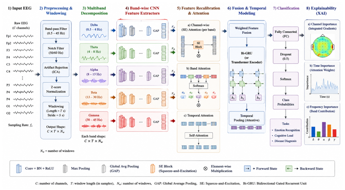
Figure 2.
Training behavior of SpectraXAI: (a) training and validation loss; (b) validation balanced accuracy and macro-F1. Loss decreases steadily while validation metrics stay high.
Figure 2.
Training behavior of SpectraXAI: (a) training and validation loss; (b) validation balanced accuracy and macro-F1. Loss decreases steadily while validation metrics stay high.
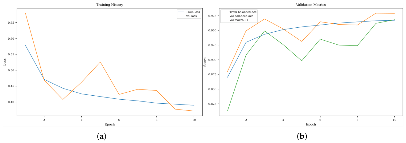
Figure 3.
Class-wise precision, recall, and F1-score on the subject-level test set. Recall is high for all four classes; the main trade-off is lower precision for SCZ, driven by false positives from healthy windows.
Figure 3.
Class-wise precision, recall, and F1-score on the subject-level test set. Recall is high for all four classes; the main trade-off is lower precision for SCZ, driven by false positives from healthy windows.
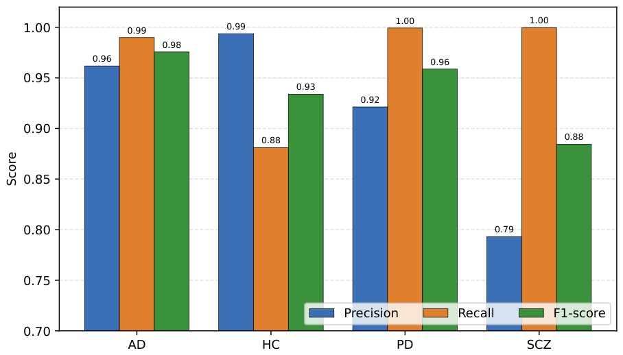
Figure 4.
Classification and representation analysis: (a) confusion matrix, with strong diagonal dominance; (b) t-SNE of the learned embeddings, showing class-separable clusters.
Figure 4.
Classification and representation analysis: (a) confusion matrix, with strong diagonal dominance; (b) t-SNE of the learned embeddings, showing class-separable clusters.
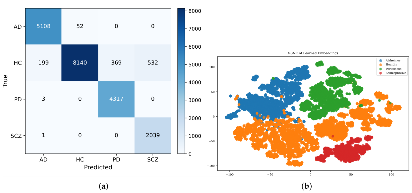
Figure 5.
Ablation results. The frequency-aware attention design lifts every metric well above the convolutional baseline on the same band-decomposed input.
Figure 5.
Ablation results. The frequency-aware attention design lifts every metric well above the convolutional baseline on the same band-decomposed input.
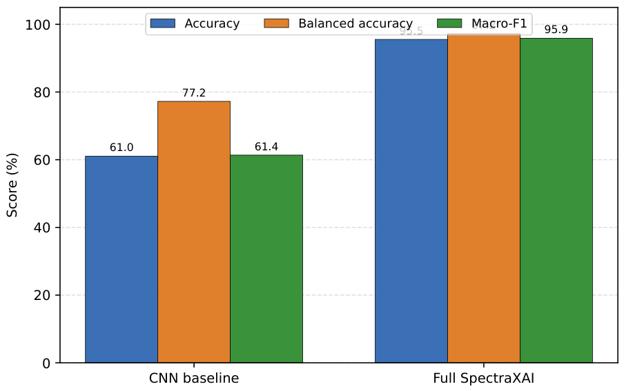
Figure 6.
Validation convergence of SpectraXAI and the convolutional baseline over training epochs: (a) macro-F1; (b) balanced accuracy. The baseline saturates early at a much lower level.
Figure 6.
Validation convergence of SpectraXAI and the convolutional baseline over training epochs: (a) macro-F1; (b) balanced accuracy. The baseline saturates early at a much lower level.
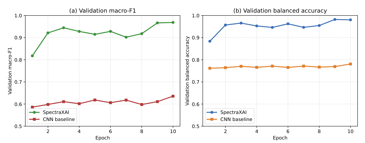
Figure 7.
Temporal explainability: (a) class-wise temporal attention; (b) Grad-CAM temporal relevance for a representative prediction. Attention shows global class relevance while Grad-CAM localizes the time regions behind a single decision.
Figure 7.
Temporal explainability: (a) class-wise temporal attention; (b) Grad-CAM temporal relevance for a representative prediction. Attention shows global class relevance while Grad-CAM localizes the time regions behind a single decision.
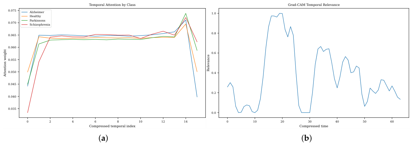
Figure 8.
Class-wise feature-attention heatmaps across EEG bands and learned convolutional channels. The model learns a different frequency-feature relevance pattern for each class.
Figure 8.
Class-wise feature-attention heatmaps across EEG bands and learned convolutional channels. The model learns a different frequency-feature relevance pattern for each class.
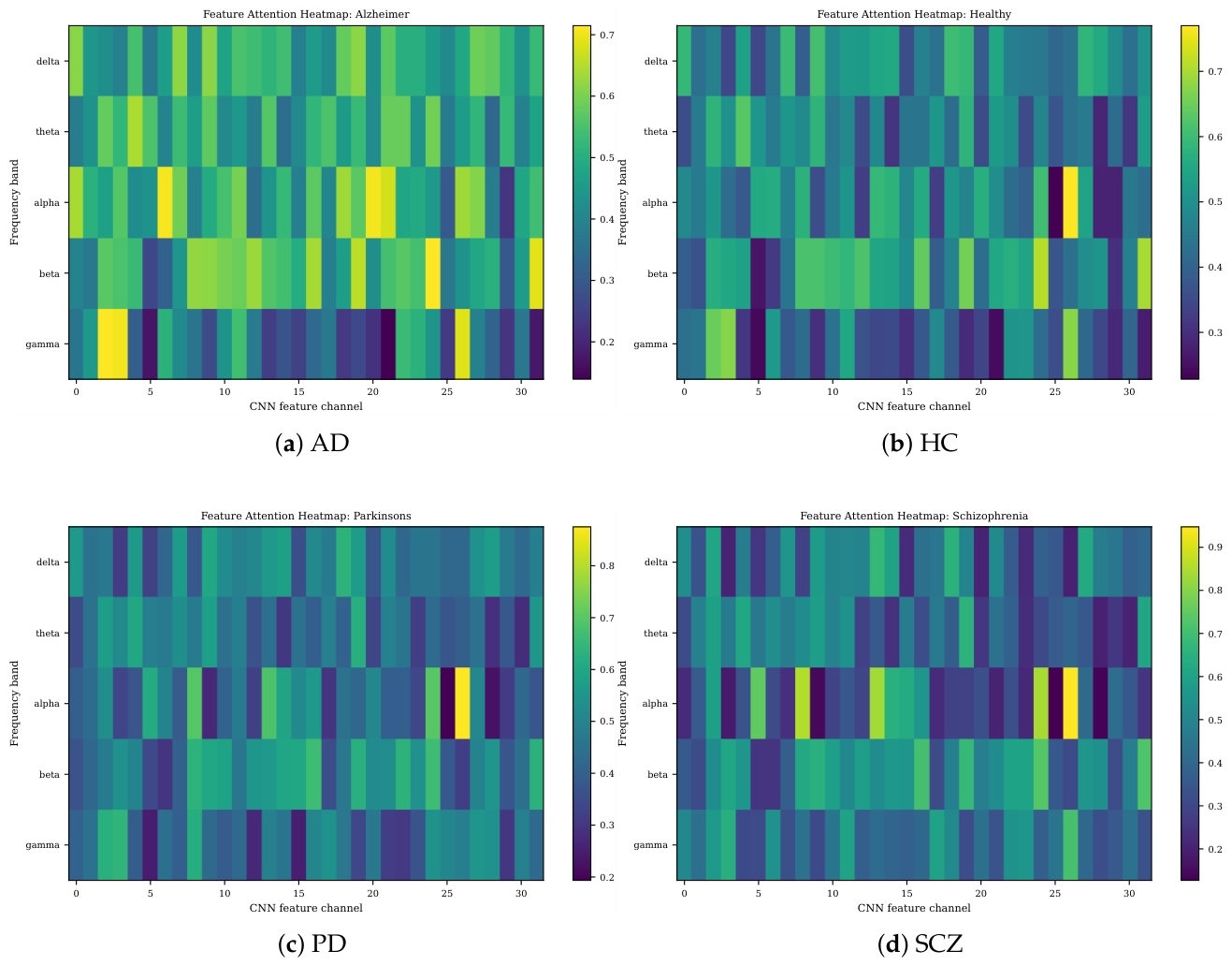

Table 1.
Composition of the combined EEG dataset.
| Source dataset | Classes used | Reference |
|---|---|---|
| Resting-state PD | PD, HC | [35] |
| Routine dementia | AD, HC | [36] |
| Resting-state SCZ | SCZ, HC | [37] |
Table 2.
EEG frequency bands used for decomposition and their typical associations.
| Band | Range (Hz) | Typical association |
|---|---|---|
| Delta () | 0.5–4 | Deep sleep; increased power in neurodegeneration |
| Theta () | 4–8 | Memory and drowsiness; elevated in dementia |
| Alpha () | 8–13 | Relaxed wakefulness; posterior rhythm |
| Beta () | 13–30 | Active cognition; motor-related activity |
| Gamma () | 30–45 | Sensory and integrative processing |
Table 3.
Layers of a single band branch and the fusion stage. Output shapes are given as channels × time for one window.
Table 3.
Layers of a single band branch and the fusion stage. Output shapes are given as channels × time for one window.
| Stage | Operation | Output shape |
|---|---|---|
| Input | one band, 19 channels | |
| Conv block 1 | Conv1d(), BN, ELU, dropout, max-pool(4) | |
| Conv block 2 | Conv1d(), BN, ELU, dropout, max-pool(4) | |
| Feature attention | squeeze-and-excitation over 32 channels | |
| Projection | Conv1d(), BN, ELU, adaptive avg-pool(16) | |
| Band attention | softmax fusion over 5 branches | |
| Temporal attention | softmax over 16 time steps | 32 |
| Classifier | Linear(32,64), BN, ELU, dropout, Linear(64,4) | 4 |
Table 4.
Training and preprocessing hyperparameters.
| Setting | Value |
|---|---|
| Sampling rate | 256 Hz |
| Window length / samples | 4 s / 1024 |
| Window overlap | 0.25 |
| Channels | 19 |
| Frequency bands | 5 (delta–gamma) |
| Optimizer | AdamW |
| Learning rate | |
| Weight decay | |
| Batch size | 32 |
| Epochs | 10 |
| Label smoothing | 0.08 |
| Gradient-norm clip | 1.0 |
| Learning-rate schedule | reduce on validation macro-F1 plateau |
| Imbalance handling | weighted random sampler |
| Augmentation (train only) | Gaussian noise, time shift, channel and band dropout |
Table 5.
Parameter budget of SpectraXAI and the convolutional baseline.
| Component | Parameters |
|---|---|
| Band branch (per band) | 14,820 |
| Five band branches | 74,100 |
| Band-attention scorer | 24,673 |
| Temporal-attention module | 1,569 |
| Classifier head | 2,500 |
| Full SpectraXAI | 102,842 (≈ 0.10 M) |
| Convolutional baseline | 17,700 (≈ 0.02 M) |
Table 6.
Subject-level split used for training, validation, and testing.
| Split | Subjects | AD | HC | PD | SCZ |
|---|---|---|---|---|---|
| Train | 552 | 138 | 245 | 115 | 54 |
| Validation | 139 | 35 | 62 | 29 | 13 |
| Test | 173 | 43 | 77 | 36 | 17 |
Table 7.
Epoch-by-epoch training and validation metrics of SpectraXAI.
| Epoch | Train loss | Train bal. acc. | Val loss | Val acc. | Val bal. acc. | Val macro-F1 |
|---|---|---|---|---|---|---|
| 1 | 0.578 | 0.870 | 0.644 | 0.794 | 0.884 | 0.818 |
| 2 | 0.470 | 0.928 | 0.448 | 0.926 | 0.957 | 0.921 |
| 3 | 0.443 | 0.943 | 0.419 | 0.942 | 0.966 | 0.944 |
| 4 | 0.427 | 0.951 | 0.457 | 0.918 | 0.953 | 0.928 |
| 5 | 0.416 | 0.957 | 0.475 | 0.905 | 0.946 | 0.915 |
| 6 | 0.409 | 0.959 | 0.427 | 0.936 | 0.962 | 0.928 |
| 7 | 0.404 | 0.962 | 0.487 | 0.906 | 0.946 | 0.902 |
| 8 | 0.397 | 0.965 | 0.450 | 0.920 | 0.955 | 0.918 |
| 9 | 0.395 | 0.965 | 0.364 | 0.972 | 0.982 | 0.967 |
| 10 | 0.389 | 0.968 | 0.367 | 0.969 | 0.980 | 0.969 |
Table 8.
Overall test performance of SpectraXAI with 95% Wilson confidence intervals over 20,760 test windows.
Table 8.
Overall test performance of SpectraXAI with 95% Wilson confidence intervals over 20,760 test windows.
| Metric | Score | 95% CI |
|---|---|---|
| Accuracy | 94.43% | [94.11, 94.73] |
| Balanced accuracy | 96.74% | [96.49, 96.97] |
| Macro-precision | 91.74% | — |
| Macro-recall | 96.74% | — |
| Macro-F1 | 93.82% | [93.48, 94.14] |
Table 9.
Class-wise test performance of SpectraXAI.
| Class | Precision | Recall | F1-score | Support |
|---|---|---|---|---|
| AD | 0.9618 | 0.9899 | 0.9756 | 5160 |
| HC | 0.9937 | 0.8810 | 0.9339 | 9240 |
| PD | 0.9213 | 0.9993 | 0.9587 | 4320 |
| SCZ | 0.7931 | 0.9995 | 0.8844 | 2040 |
| Macro average | 0.9174 | 0.9674 | 0.9382 | 20760 |
| Weighted average | 0.9510 | 0.9443 | 0.9446 | 20760 |
Table 10.
Ablation comparison between the convolutional baseline and the full SpectraXAI model.
| Model | Accuracy | Balanced Acc. | Macro-F1 | Params |
|---|---|---|---|---|
| Convolutional baseline | 61.02% | 77.24% | 61.36% | 0.02 M |
| Full SpectraXAI | 95.55% | 97.23% | 95.88% | 0.10 M |
Table 11.
Compact comparison of representative studies with SpectraXAI.
| Ref. | Task / modality | Method | Key limitation |
|---|---|---|---|
| [1,38] | PD / AD detection from EEG | CNN, LSTM, temporal CNN with attention and XAI | Mostly binary or disease-specific |
| [28,29] | AD / dementia EEG classification | CSP with random forest; PSD and connectivity with SVM; SHAP/LIME | Relies on handcrafted features |
| [6,7] | SCZ detection | CNN, wavelet-CNN, attention CNN | Binary SCZ-versus-control |
| [5] | Epilepsy EEG classification | Spectrogram images with CNN backbones | Single-disorder binary task |
| [8,20,24] | General EEG decoding | Transformer and graph networks | High accuracy without a multi-disorder screening focus |
| [25,26] | EEG foundation models | Large-scale self-supervised pre-training | Data-hungry and hard to interpret |
| [10] | PD diagnosis from voice-related EEG | Interpretable graph learning | Single disorder |
| SpectraXAI | Four-class EEG: AD, healthy, PD, SCZ | Multi-band CNN with SE, band and temporal attention, Grad-CAM | EEG-only, multi-class, subject-level, explainable, 0.10 M params |
Disclaimer/Publisher’s Note: The statements, opinions and data contained in all publications are solely those of the individual author(s) and contributor(s) and not of MDPI and/or the editor(s). MDPI and/or the editor(s) disclaim responsibility for any injury to people or property resulting from any ideas, methods, instructions or products referred to in the content. |
© 2026 by the authors. Licensee MDPI, Basel, Switzerland. This article is an open access article distributed under the terms and conditions of the Creative Commons Attribution (CC BY) license (http://creativecommons.org/licenses/by/4.0/).
Copyright: This open access article is published under a Creative Commons CC BY 4.0 license, which permit the free download, distribution, and reuse, provided that the author and preprint are cited in any reuse.