

Submitted:
09 October 2026
Posted:
12 October 2026
You are already at the latest version
Abstract
We study the joint kernel of operators that replace an ordinary tensor factor by an odd marker. In characteristic zero its decomposition deletes the first column of each site partition. Over every field, ballot words describe the leading words of every socle layer and give dimensions independent of the characteristic. The closed cochains form a free associative algebra generated by prime ballot words; we determine its hook-shaped generator multiplicities. A Grassmannian evaluation map gives exact polynomial-exponential growth below the free range. A cyclic frame reduces group-invariant closure to one equation. The Cartan complex identifies exterior-algebra Ext with the homology of row-bounded rook complexes. Their top cycles have field-independent dimension, so the next integral homology group is torsion-free. For rectangular chessboards this proves the torsion-free half of a conjecture of Shareshian and Wachs on higher chessboard homology and, together with known torsion results, completes their criterion for torsion in bottom homology.
Keywords:
closed tensor cochains
; ballot words
; free associative algebras
; super Schur–Weyl duality
; Grassmannians
; chessboard complexes
; Shareshian–Wachs conjecture
; algebraic combinatorics
2020 Mathematics Subject Classification. Primary 05E10, 16S10; Secondary 05E45, 14M15, 16W22, 17B10, 20C30, 55U10.
1. Introduction
For a covector ϕ ∈ W*, let dϕ act on (W⊕Ke)⊗n by replacing an ordinary tensor factor w by the odd marker ϕ(w)e, with the Koszul sign. We study the joint kernel in marker degree p. In characteristic zero, the Sμ-multiplicity space is in degree p = 𝓁(μ) and zero in the other degrees, where μ− is obtained by deleting the first column of μ. This Column Law separates the site combinatorics from the invariant theory of any group acting on W.
The characteristic-free form replaces the decomposition by a ballot condition on leading words. It gives the dimension of every content space and every socle layer over an arbitrary field. In multilinear content, these spaces are top cycles of complete chessboard complexes. Their field-independent dimensions imply that is free for every 1 ≤ m ≤ n. This includes the two boundary families n = 2m − 4,2m − 3 left open in the bottom-homology torsion criterion of Shareshian and Wachs [27, §§7,11], and proves the torsion-free implication of their higher-degree conjecture [27, Conjecture 7.4].
The Schur–Weyl and Pieri rules and the transposition class-sum scalar are classical [9,12,17,20,23]. Berele–Regev [1] and Sergeev [26] provide the super Schur–Weyl setting; see also Cheng–Wang [4]. Related content factors appear in the Pieri inclusions of Olver [21], Sam–Weyman [24], and Eisenbud–Fløystad–Weyman [6]. Marko [18,19] studies even-primitive vectors, meaning highest vectors for the even subgroup [18, §1.5]. Our joint kernel consists instead of invariants of the odd nilradical and contains an entire GL(W)-module in its highest marker degree.
The group-dependent step is Lemma 2.2: on invariant cochains, a frame whose orbit spans W* detects every contraction. In degree one this identifies invariant closed cochains with symmetric invariants; higher degrees are controlled by invariant multiplicities of Schur functors.
Organisation. Section 2, Section 3 and Section 4 prove the Column Law in characteristic zero, compute the content spectrum, and treat invariant closed cochains. Section 5 establishes the characteristic-free leading-word and socle formulas. Section 6 determines free generators and their hook multiplicities; Section 7 gives the free-range dimensions and Grassmannian evaluation. Section 8 treats smaller orbit spans and several markers. Section 9 applies the formulas to chessboard and row-bounded rook homology. Section 10 and Section 11 record the computations and open questions.
1.1. Conventions
Unless stated otherwise, K is a field of characteristic zero, W is a finite-dimensional K-vector space, and G acts linearly on W. The group may be finite, algebraic, or a specified subgroup of GL(W); no averaging over G is used. Section 5 and Section 9, the freeness and multigraded dimension statements of Section 6, and Proposition 8.4 hold over every field. Schur-module decompositions and Grassmannian evaluation use characteristic zero, except for the good-characteristic extension in Proposition 3.2. Numerical joint-kernel dimension formulas extend to every field by Theorem 5.5. Schur functors vanish when their partitions have more than dimW rows.
We write 𝓁(λ) for the number of nonzero parts of a partition and θ ∈ W* for the fixed frame.
Write [n] = {1,…,n}, m = n − p, Sλ for a Specht module, and 𝕊λW for a Schur functor. We use the English convention for Young diagrams and the content
For a set of sites T, write WT for the tensor product with those site labels. Write Cc for the complement of C in [n]. All tensor slots are labelled by sites. An odd marker has degree one; an element of W has degree zero. Permutations of sites use the resulting Koszul signs.
Table 1 records the spaces and actions used throughout the paper.
The fixed-frame operator is not generally a differential on G-invariants. Accordingly, our theorem concerns closed cochains and a joint kernel; it does not identify the cohomology of an invariant subcomplex.
2. The Site Construction and the Column Law
The site construction keeps the orientation of the marked slots separate from the ordinary tensor factors. Define
The orientation of C = {c1<…<cp} is . Equivalently, (2.1) is the component with p odd markers of (W⊕Ke)⊗n. For θ ∈ W*, the map replaces a slot wj by ej, multiplies by θ(wj), and attaches the sign
(−1)|{i∈C:i<j}|.
Summing this operation over the unmarked sites defines dθ. The two orders of marking distinct sites have opposite signs. Hence , and more generally dϕdψ + dψdϕ = 0.
Set
Call θ a cyclic frame if spanK(Gθ) = W*. In particular, a nonzero frame is cyclic when W* is irreducible.
Theorem 2.1 (Column Law). Let 0 ≤ p ≤ n. There is an isomorphism of GL(W) × Sn-modules
If θ is a cyclic frame, then
Here λ + (1p) means addition of one box to each of the first p rows, padding λ with zeros. Thus the operation adds a column of height p to the left of the diagram after the usual row alignment. The empty partition and p = 0 are interpreted in the evident way.
Lemma 2.2 (Orbit amplification). Under the cyclic-frame hypothesis,
Proof. Naturality gives gdθg−1 = dgθ. If v is fixed by G and dθv = 0, then dgθv = 0 for every g ∈ G. Linearity in the covector and the spanning condition imply dϕv = 0 for all ϕ. The reverse inclusion is immediate. □
The lemma identifies exactly where the group is used. Everything needed to determine is group-free.
2.1. Column Deletion and the Super Tensor Interpretation
For a partition μ, let μ− denote the partition obtained by deleting its first column and discarding zero rows. If 𝓁(λ) ≤ p, then μ = λ + (1p) has exactly p rows and μ−=λ. Consequently, Theorem 2.1 has the equivalent form
Summing over p,
Each partition μ indexes one summand in (2.8), in degree p = 𝓁(μ). The nonzero summands satisfy 𝓁(μ−)≤d, equivalently μd+1 ≤ 1, where d = dimW: this is the (d,1)-hook of super Schur–Weyl duality [1,26]. In the tensor power of W⊕Ke, the Column Law selects the GL(W) multiplicity space obtained by first-column deletion. Table 2 illustrates the decomposition at n = 5.
By cochain degree p = 0,…,5, the same total is 0 + 15 + 80 + 51 + 12 + 1 = 159. Here 𝕊∅W = K; the p = 0 joint kernel is zero for n > 0, while .
Remark 2.3 (Odd nilradical and a second proof). Put V = W⊕Ke and 𝔤 = 𝔤𝔩(W|Ke). Its type-I grading has 𝔤+1 = Hom(W,Ke), 𝔤0 = 𝔤𝔩(W)⊕𝔤𝔩(Ke), and 𝔤−1 = Hom(Ke,W) [13]. For φ ∈ W*, the element Xφ ∈ 𝔤+1 sends w to φ(w)e and kills e. Its tensor action is exactly dφ: the odd coproduct sign is (2.2). Consequently, the direct sum in (2.8) is .
In characteristic zero, super Schur–Weyl duality decomposes V⊗n as ⨁μLμ⊗Sμ, where the nonzero Lμ are the irreducible covariant tensor modules indexed by the (d,1)-hook [1,4,26]. Grade each Lμ by the number of odd factors. If a nonzero homogeneous has degree a, PBW gives (𝔤)v = (𝔤−1)(𝔤0)v, which has degrees at most a. Irreducibility therefore forces a to be the top degree. Conversely, every vector in that top degree is killed by 𝔤+1, since this subalgebra raises degree. The invariant space is graded, so this accounts for every invariant vector.
The hook Schur character in one odd variable is
The largest possible exponent of y is 𝓁(μ), attained uniquely by ν = μ−; its coefficient is . Thus as a GL(W)-module, in degree 𝓁(μ), proving (2.7). The rational tensor action, Young projectors, multiplicity spaces, and contraction kernels commute with scalar extension, giving the identification over every characteristic-zero field. Section 3 supplies an independent proof and the additional information of every content eigenvalue.
3. Proof by a Content Operator
The Column Law is the zero-eigenvalue part of a natural content operator. Its other eigenvalues give an exact spectral bound.
3.1. The Sum of Squares
First work over ℝ and choose an orthonormal basis w1,…,wd of W. Give the oriented tensor basis of (2.1) the corresponding positive inner product. Put and
Then : the last equality follows because φ ↦ dφ is linear, so it suffices to test a basis. Although (3.1) uses an inner product, the next expression shows that H is natural in W.
Lemma 3.1. On ,
The transposition in this formula is the signed site transposition, and the set of mixed pairs is evaluated on each summand of (2.1).
Proof. Contracting and then restoring the same site contributes one copy of the identity for each of the m unmarked sites. Contracting one site and restoring a different marked site exchanges those two sites. The marker passes the markers between them with the Koszul sign, while the two differential signs supply the additional minus sign in (3.2). These exhaust the terms in . □
Under the sign identification of Lemma 9.1, H on the content-(1m) subspace of is the top-degree chessboard Laplacian ∂t∂ studied by Friedman and Hanlon [8].
3.2. Pieri Decomposition and Content Scalars
Schur–Weyl duality and induction give
By the exterior Pieri rule [9,17,23], each induced factor is the multiplicity-free sum of Sμ for which μ/λ is a vertical p-strip, with at most one new box in each row. Thus the nonzero (λ,μ) blocks are irreducible for the product action.
Let . On each oriented summand of (2.1), split the pairs into marked–marked, unmarked–unmarked, and mixed pairs. A restriction to one fixed marking set is not by itself a globally Sn-equivariant operator; the marking set is transported with the summand. The marked–marked contribution is the global scalar . The unmarked–unmarked contribution is the central class sum of , acting by c(λ) on the unmarked λ-type. Finally Ωn acts by c(μ) on total site type μ [12,20]. Subtracting these actions in (3.2) is therefore well defined and gives
3.3. The Zero Eigenvalue
Write the rows receiving new boxes as r1<…<rp, padding λ with zeros. The new box in row r has content λr + 1 − r. Substitution in (3.4) gives
Both summands are nonnegative integers. Equality holds precisely when rj = j for every j, and every box of λ lies in those first p rows. Thus
hλ,μ = 0 ⇔ 𝓁(λ) ≤ p and μ = λ + (1p).
Since H is a sum of squares, its zero eigenspace is exactly the joint kernel. This proves (2.4) over ℝ. All contraction matrices, site permutations, and characteristic-zero Young decompositions used here are defined over ℚ. Equality of their kernels therefore extends to every characteristic-zero field by scalar extension. Taking G-fixed vectors and using Lemma 2.2 proves (2.5). □
The positive inner product determines a universal rational kernel, so no invariant form on W is needed.
3.4. The Exact Spectral Radius and Good Characteristic
Proposition 3.2. Put m = n − p and d = dimW ≥ 1. Every ambient Pieri block satisfies
0 ≤ hλ,μ ≤ m + p𝓁(λ) ≤ m + pmin(d,m).
The last bound is attained. Thus the spectral radius is m + pmin(d,m); the dimension-independent bound (p + 1)m is attained whenever d ≥ m. If charK > n, the decompositions (2.4), (2.7) and the cyclic-frame formula (2.5) remain valid; this assertion uses Theorem 5.5 below.
Proof. Put r = 𝓁(λ). In (3.5), the jth added box lies in a row rj ≤ r + j. Hence hλ,μ ≤ m + pr. Equality holds exactly when the new boxes occupy rows r + 1,…,r + p, equivalently μ = (λ,1p). A partition of m of length min(d,m) exists when m > 0; use the empty partition when m = 0. Appending p rows realises the bound. The earlier bound follows from min(d,m) ≤ m.
For the characteristic assertion, work with the integral tensor lattice localised at n!. The Young projectors and the Schur–Weyl decomposition are defined there. On reducing modulo q > n, the relevant symmetric-group algebras and polynomial Schur algebras are semisimple [9,23]. The stacked map is GL(W) × Sn-equivariant, so its kernel splits according to those ambient domain types. Each restricted contraction matrix can only lose rank under reduction. Theorem 5.5 says that the sum of their kernel dimensions does not increase. Therefore no projected kernel dimension increases, and the characteristic-zero block multiplicities persist. Lemma 2.2 then gives the invariant formula without any averaging over G. This assertion concerns the joint contraction kernel; kerH need not equal it in positive characteristic. □
3.5. A Complete Small Block
For p = 2 and λ = (2,1), the induced site representation has dimension . Table 3 gives the dimensions and eigenvalues of all four Pieri summands.
Figure 1 shows their added strips and the surviving first column.
4. The Invariant Degree-One Poincaré Lemma
The one-marker case identifies invariant closed cochains with symmetric invariants. A comparison with the single-frame kernel shows why cyclicity is needed.
Corollary 4.1. If θ is cyclic, then
and Sn acts trivially on this space.
Proof. The only partition of n − 1 with at most one row is (n − 1). Its column extension is (n), which affords the trivial representation. □
We use the normalised symmetrisation map, with r ≥ 0,
Here Pol0(1) = 1. If qr:W⊗r → SymrW is the quotient map, then qrPolr = id, while Polrqr is the averaging projector. We abbreviate Polr to Pol when the degree is clear.
For P ∈ Symn−1W, put Poln−1(P) in the slots other than i, with marker ei, for every i. The two contractions contributing to a two-marker component cancel. Under cyclicity, Corollary 4.1 makes this a bijection onto invariant closed cochains; its inverse applies qn−1 to any vertex component. Equivalently, P is a homogeneous invariant polynomial on W*; polynomials on W require replacing W by its dual.
Example 4.2 (Failure without a cyclic frame). Let G be trivial, let W = Kx⊕Ky, and let θ(x) = 1, θ(y) = 0. At n = 2, p = 1, a cochain is a pair (u,v) ∈ W⊕W, and closure imposes only θ(v − u) = 0. The closed space has dimension three. The diagonal polarisation image has dimension two. For example, (y,0) is closed and is not diagonal. Thus invariance alone does not suffice; the orbit-spanning condition cannot be omitted.
The same proof gives the dimension formula
For p = 1, all dimension growth is therefore controlled by the Hilbert series of symmetric invariants. For higher p, the required data are invariant multiplicities of Schur functors, not merely dimensions of symmetric powers.
4.1. The Size of a Single-Frame Kernel
Proposition 4.3 (Single-frame kernel). Let d = dimW ≥ 1, let θ ≠ 0, and put . Then
Proof. Choose u ∈ W with θ(u) = 1. As a two-term complex, V = W⊕Ke with Δθ(w) = θ(w)e splits as . The oriented site complex is V⊗n with its total differential. Künneth therefore gives H0 = (kerθ)⊗n and Hp = 0 for p ≥ 1. In positive degree the kernel is the preceding image, whose dimension is . This proves (4.4), with the usual empty-tensor convention when n = 0. □
For Example 4.2, the single-frame kernel has dimension 4 − 1 = 3, whereas the joint kernel has dimension two. Table 4 gives further comparisons on the full cochain space.
For d = 3 and p = 2, the recurrence and the hook formulas simplify to
At n = 2, the factor 2n−3 = 1/2 still gives the joint-kernel dimension 1. For the last identity, write λ = (n − 2 − b,b). Its contribution is . Pairing b with n − 1 − b and using the binomial second moment gives (4.5). The ambient and single-frame dimensions have exponential base three, while the joint kernel has base two; the joint-to-ambient ratio is exactly (2/3)n−2.
5. Characteristic-Free Leading Words and Socle Layers
We now describe the joint kernel and every layer of its socle filtration by leading words. Let K be any field, W = Kd, and order the alphabet by e < 1<…<d, with e odd and the letters even. We take the lexicographically largest supported word as the leading word LW(x).
For a letter a, let
For a word u, let Eu(j)=#{i > j:ui = e}. Write (k) for the words satisfying
for every strictly increasing subsequence of nonmarker letters, with j1<…<jt. Set = (1); its elements are called ballot words (the term refers to (5.1), not the classical Yamanouchi condition). For p ≥ 0 and α ∈ ℕd with p + |α| = n, let k;p,α be the words in (k) having p markers and nonmarker content α, and put p,α = 1;p,α. The condition concerns all increasing subsequences, not only adjacent runs.
t ≤ k − 1 + Eu(j1)
Lemma 5.1 (the marker-free tail). Let 0 ≠ x ∈ sock(n) and u = LW(x). If an increasing subsequence starts at j1 and no marker occurs after j1, its length is at most k − 1.
Proof. Suppose its first k letters are a1<…<ak, in positions j1<…<jk. Replace these letters by markers to obtain ω. A word contributing to the coefficient of ω in dSx, where S = {a1,…,ak}, is obtained by restoring these k letters in marker positions of ω. Every original marker of u lies before j1. Restoring a letter in such a position produces a word larger than u. If only the positions j1,…,jk are used, the increasing assignment is the lexicographically smallest assignment of the k distinct letters. Thus every assignment except the original one again gives a larger word. Only u contributes, with coefficient ±xu ≠ 0. This contradicts dSx = 0. □
Lemma 5.2 (deleting a marker). For a position f, define
Proof. The socle conditions are homogeneous in marker degree, so it suffices to take x homogeneous of marker degree p. Move slot f to the last position by the signed permutation of tensor factors. The signed adjacent interchange is τ(v⊗w) = (−1)|v||w|w⊗v. Substitution in the Koszul rule d(v⊗w) = dv⊗w + (−1)|v|v⊗dw gives τd = dτ term by term; composing adjacent interchanges proves the same for the slot move. Write the resulting tensor as
Indeed, at most one contraction can act in the final slot. In the term arising from , the first i − 1 contractions act in the left factor, changing its parity from p to p + i − 1. Applying the i-th contraction in the final slot therefore contributes (−1)p+i−1 by the Koszul rule. Every later contraction again acts in the left factor, with no further tensor-product sign. Since dSτx = 0, every ya belongs to sock(n − 1). For a set T of size k + 1, choose t ∈ T and apply dt to (5.2) with S = T∖{t}. Every term on its right contains k distinct contractions applied to some ya, and therefore vanishes. Hence dTy = 0. □
Theorem 5.3 (leading-word bound). Over every field,
LW(sock(n)∖{0}) ⊆ (k).
Proof. Induct on n, the empty word being immediate. Let u = LW(x). If u contains no marker, Lemma 5.1 applies to every increasing subsequence. Otherwise let f be its last marker. A subsequence starting after f again satisfies the required bound by Lemma 5.1. For a subsequence starting before f, use Lemma 5.2. Among words having a marker in slot f, deletion of that slot is injective and preserves lexicographic order. The coefficient of u∖f in is exactly . Consequently
The Robinson–Schensted–Knuth (RSK) correspondence, using ordinary row insertion [23,25], gives a count uniform in the socle index. Write Kνα for the number of semistandard tableaux of shape ν and content α, and fμ for the number of standard tableaux of shape μ.
Proposition 5.4 (standardised RSK). Fix a word u with p markers. Replace its i-th marker from the right by εi, where
εp<…<ε1 < 1<…<d.
Apply ordinary row insertion to the resulting word read from right to left, obtaining an insertion tableau P(u), a recording tableau R(u) and a shape μ(u). The marker entries of P(u) occupy exactly the first p boxes of its first column. Moreover,
For k = 1 this gives SSYT(λ,α) × SYT(λ + (1p)), summed over λ⊢n − p with 𝓁(λ) ≤ p.
Proof. Restricting an insertion tableau to its smallest symbols gives the insertion tableau of their subword. Here that subword is ε1,…,εp, which is strictly decreasing, so its tableau is the first-column shape (1p).
By Schensted’s theorem [25], 𝓁(μ(u)) is the longest strictly decreasing subsequence in the reversed standardised word. Such a subsequence consists of letters followed by markers. Reading its letters in the original order gives a strictly increasing subsequence starting at j1, of some length t. Every marker to the left of j1 can then be included: they occur in decreasing order and are smaller than every letter. The longest length is therefore
To verify surjectivity in (5.3), start with any displayed pair (T,R). Fill the removed column, from top to bottom, by εp,…,ε1. The result is an ordinary semistandard tableau P, because every marker is smaller than every letter. Inverse RSK applied to (P,R) recovers a word whose marker subword has insertion tableau a single column. Since the marker symbols are distinct, that subword is necessarily ε1,…,εp in this order. Reverse the recovered word and replace all εi by e. This is precisely the standardisation convention above and gives the unique inverse. The row bound identifies the words in k;p,α.
When k = 1, the marker column forces 𝓁(μ) = p. Subtracting one box from each of these rows gives λ, and shifting the remaining tableau one column to the left identifies its skew shape with λ. □
The Pieri rule gives
Theorem 5.5 (characteristic-free Column Law). For every field K, every n,p ≥ 0, and every nonmarker content α ∈ ℕd with p + |α| = n,
Proof. Gaussian elimination identifies the dimension of a subspace with the number of its possible leading words. Theorem 5.3 and the case k = 1 of Proposition 5.4 therefore bound the left side of (5.4) above by its stated right side. Over ℚ, equality is the weight-space form of the characteristic-zero Column Law. On each content space the stacked contraction matrix has integer entries. Reduction modulo a prime can only decrease its rank, so its kernel over that prime field has dimension at least its rational kernel dimension. Extension of the coefficient field preserves rank. The upper and lower bounds coincide in every characteristic, forcing both the dimension formula and equality of the leading-word sets. □
Theorem 5.6 (characteristic-free socle series). For every field K, every k ≥ 1 and every n,p,α as in Theorem 5.5,
LW(sock(n)p,α∖{0}) = k;p,α,
In particular, the dimensions of every socle term and every successive socle quotient are independent of the field.
Proof. First work in characteristic zero. Under super Schur–Weyl duality, write V⊗n = ⨁μLμ⊗Sμ, with μd+1 ≤ 1. Grade Lμ by the number of markers. The hook-Schur branching formula gives
Let 𝔤 = 𝔤𝔩(W∣Ke) and write 𝔤 = 𝔤−1⊕𝔤0⊕𝔤+1, where 𝔤+1 consists of the contractions. It is odd abelian, with enveloping algebra Λ(𝔤+1), and raises marker degree by one. Suppose 0 ≠ v ∈ Lμ[p] is annihilated by all products of k contractions. Longer products annihilate it as well. The PBW theorem, ordered with the raising part acting first, gives
(𝔤)v = (𝔤−1)(𝔤0)Λ<k(𝔤+1)v.
Every vector on the right has marker degree at most p + k − 1. Irreducibility implies (𝔤)v = Lμ, so p + k − 1 ≥ 𝓁(μ). Conversely, every vector of degree p ≥ 𝓁(μ) − k + 1 is killed by k contractions, since they would raise its degree above the largest one present. It follows that
Combining (5.6), the branching formula and the multiplicity fμ proves (5.5) over ℚ. Partitions outside the (d,1) hook contribute zero to its right side because every associated Kostka number is zero.
For an arbitrary field, Theorem 5.3 and Proposition 5.4 now give
dimKsock(n)p,α ≤ |k;p,α| = dimℚsock(n)p,α ≤ dimKsock(n)p,α.
The last inequality follows from the integer matrix obtained by stacking all dS with |S| = k, exactly as in Theorem 5.5. Equality throughout proves both assertions. Subtracting the dimensions of successive terms proves the claim about the quotients. □
The empty-partition conventions cover n = p = 0. If d = 0, the only word is en; if k > d, the intersection defining sock is the whole tensor power and every word satisfies the ballot inequality. Formula (5.5) includes both cases.
6. The Algebra of Closed Cochains
Let , including , and let 𝒵+ be its augmentation ideal. Since each contraction is a parity-skew derivation, concatenation makes 𝒵 a graded subalgebra of T(W⊕Ke). Write
6.1. Prime Ballot Words
A nonempty ballot word is prime if it is not the concatenation of two nonempty ballot words. Denote the set of prime ballot words by Π.
Theorem 6.1 (freeness). For each π ∈ Π, choose a closed cochain gπ with leading word π, homogeneous in its length, marker number and letter content. Then the elements gπ freely generate 𝒵.
Proof. Every suffix of a ballot word is ballot: the number of markers to the right of the first letter of any increasing subsequence is unchanged on passing to a suffix. Ballot words are also closed under concatenation. Indeed, split an increasing subsequence in uv into its portions in u and v; their lengths are bounded by the relevant markers in u and by the total number of markers in v, respectively.
Consequently, a ballot word is prime precisely when it has no proper nonempty ballot prefix. Factoring at the shortest nonempty ballot prefix, and repeating on the remaining suffix, gives a unique factorisation into primes. Equivalently, the prime words form a prefix code, and the ballot monoid is the free monoid on Π.
Leading words multiply under concatenation. Thus distinct products of the gπ have distinct leading words, namely the distinct ballot words, and are linearly independent. In each multidegree, the characteristic-free leading-word theorem says that their number is dim𝒵 in that multidegree. They therefore form a basis. □
Let (t,u;w) be the character series of 𝒵, where t records length, u records marker number and w records letter content. Then
Proposition 6.2 (support). If p ≥ 2, then for n < 2p.
Proof. For a prefix u, let
Δ(u) = max(0, t−#{markers to the right of j1 in u}),
where the maximum ranges over all strictly increasing subsequences of letters. Proposition 5.4 identifies this deficit with 𝓁(μ(u)) − p(u), where p(u) is the marker count. Thus u is ballot exactly when Δ(u) = 0. Appending a letter increases Δ by at most one, whereas appending a marker replaces it by max(0,Δ−1).
A prime word other than e has positive deficit at every proper nonempty prefix. Each of its p markers therefore lowers the deficit by exactly one, and its letters must supply at least p increases. It has at least p letters, so its length is at least 2p. Theorem 6.1 now gives the assertion. □
6.2. Generator Representations
Every positive-degree closed cochain has at least one marker, so the one-marker part is indecomposable. The Column Law gives
Proof. The multiplicity of 𝕊(n−2−j,j)W in is
Proposition 6.4 (Catalan diagonal). The multiplicity of ΛpW in is
Proof. A column ΛrW can occur in only when n = p + r and r ≤ p. Proposition 6.2 forces r = p for generators with p ≥ 2, while the one-marker formula gives only e and W among column-shaped generators.
A Littlewood–Richardson product can contain a column only if each factor is a column, and ΛaW⊗ΛbW contains Λa+bW with multiplicity one whenever the latter is nonzero. In a product of such generators, each non-scalar factor has length minus twice its marker number equal to zero, whereas e has this difference equal to −1. Hence e cannot occur in a product contributing to ΛpW at (n,p) = (2p,p). The Column Law gives multiplicity in . If B(z) records the corresponding generator multiplicities and , freeness gives
Theorem 6.5 (hook generators). Assume that K has characteristic zero. For p ≥ 1 and n ≥ 2p, the hook-shaped part of consists of
Proof. Work first with the stable symmetric-function character series (t,u) of 𝒵, where t records length and u records marker number. Let ρ:Λℚ → ℚ[x,y] be the ring homomorphism defined on power sums by
ρ(pj) = xj + (−1)j−1yj.
The one-even-variable, one-odd-variable specialisation of the Schur functions gives
ρ(chQ) = 1 − ρ()−1.
To compute ρ(), put for a ≥ 1, b,c ≥ 0, and put f(0,0,c) = 1. Set f = 0 on all other triples, and define
f(a,b,c) = f(a − 1,b,c) + f(a,b − 1,c + 1) + f(a,b,c − 1).
The zero convention includes the missing first-row corner when a = 1 and b > 0. Summing this recursion gives
ω2 − (1 − X)ω + v = 0, B = 1 − X − ω, v = ωB.
Substitution w = ω is valid formally and determines vΨ(X,v,0) = ω(1 − v/(1 − ω)). The two sides of the preceding functional equation then contain the factor w − ω; cancelling it and using v = ωB yields the convenient form
For a hook λ = (a,1b) in the Column Law, write c = p − 1 − b. Then λ + 1p = (a + 1,2b,1c). Consequently, with
X = xt, v = yut2, w = tu,
the specialised Column Law is
Theorem 6.5 recovers the hook part of Proposition 6.3 and the Catalan diagonal of Proposition 6.4.
For example, in characteristic zero the first generator beyond the one-marker polarisations has (n,p) = (4,2) and type Λ2W. For a,b ∈ W, a representative is
abee − aeeb − baee + beea − eabe + ebae + eeab − eeba.
In characteristic two this integral representative becomes decomposable; homogeneous generators with prime leading words are supplied by Theorem 6.1.
6.3. Hilbert Series and Invariant Algebras
Put , , and . Freeness gives . For n ≥ 1 and d = 1,
The invariant algebra 𝒵(W)G is free for every subgroup G ≤ GL(W). Choose a degreewise GL(W)-stable lift of Q to identify 𝒵(W) equivariantly with T(Q). The Lane–Kharchenko theorem [15,16], in the arbitrary-rank form of Ferreira–Murakami–Paques [7, Corollary 3.3], then gives freeness. For a cyclic frame, Lemma 2.2 identifies this algebra with the invariant closed cochains.
Figure 2 shows the support of the generator dimensions and the two-marker multiplicities, including the boundary values of Proposition 6.3.
7. The Free Range and Grassmannian Sections
The dimension formula simplifies when p ≥ d; for p < d it is realised by sections of a vector bundle on a Grassmannian.
7.1. The Free Range
Put d = dimW ≥ 1. The marker operators make (W⊕Ke)⊗n a graded module over the exterior algebra E = Λ(W*).
Proposition 7.1 (Free-range dimensions). For d ≤ p ≤ n,
Equivalently, this dimension is the coefficient of tp−d in the polynomial quotient obtained by dividing (d + t)n by (1 + t)d. Consequently,
Proof. In the super Schur–Weyl decomposition, a covariant tensor module Lμ is typical precisely when 𝓁(μ) ≥ d. For the even-first Borel, its Kac presentation is Λ(Hom(W,Ke))⊗L0, so it is free over E; its generators have marker degree 𝓁(μ) − d, and its socle has degree 𝓁(μ). These are the standard typicality and Kac-module facts for 𝔤𝔩(d|1), with the raising odd nilradical used in Remark 2.3; see Cheng–Wang [5, (2.2), Theorem 2.7 and Proposition 3.11]. The remaining summands have top marker degree 𝓁(μ) < d, by (2.9). Thus
(d + t)n = (1 + t)dGn(t) + An(t), degAn < d,
where Gn counts the generators of the typical summands, including their Specht multiplicities. In degree p ≥ d, the joint kernel is their socle, so .
Expand
Here freeness refers to the exterior-algebra action of the contractions; it is separate from the associative-algebra freeness of Section 6.
Corollary 7.2 (A primitive in the free range). Choose a basis of W* and put . For p ≥ d,
Proof. On a free E-module the joint kernel of multiplication by its generators is the image of its top exterior power. Apply this to every typical summand. Atypical summands have no component in degree p ≥ d. □
7.2. Sections on a Grassmannian
Let 1 ≤ p < d, let X = Grp(W) denote the Grassmannian of rank-p quotients of W, and let be its tautological quotient bundle. The symmetric group acts on ⊗n by ordinary place permutations.
Theorem 7.3 (Grassmannian evaluation). There is a natural GL(W) × Sn-equivariant isomorphism
Proof. The prescription is polynomial in the quotient map and is unchanged by a change of quotient frame, since the determinant factor cancels the change in the alternating tensor. Interchanging two markers changes sign on both sides, so evaluation intertwines the signed place action on the source with the ordinary place action on the target.
Schur–Weyl duality gives
It remains to show that the specified map is nonzero on each summand. First take a real vector space U of dimension p, with an orthonormal basis, and let . The free-range identity gives . Up to a fixed overall sign, evaluation at the identity quotient is the transpose Δt: the transpose contractions replace markers with the alternating basis frame. Since imΔ∩kerΔt = 0, this evaluation is injective on .
Now choose a split quotient W↠U. Its splitting induces . Every partition μ with 𝓁(μ) = p occurs in , so evaluation on W is nonzero on every summand. Schur’s lemma proves the isomorphism over ℝ. The maps and decompositions are defined over ℚ, hence the result holds over every characteristic-zero field by scalar extension. □
Corollary 7.4 (exact polynomial growth). Put D = p(d − p). There is a polynomial Pp,d(n) of degree D such that
Proof. The preceding Borel–Weil–Bott computation also proves that all higher cohomology vanishes. Hirzebruch–Riemann–Roch [10] therefore gives
For p = 1 this recovers , with n ≥ 1. At the other boundary,
Proof. A polynomial of degree D multiplied by pn has a rational generating function with denominator (1 − px)D+1; its nonzero leading coefficient prevents cancellation of that pole. The final term is the free-range series. □
The evaluation map depends on the characteristic: when p = 1, the closed cochain evaluates to 2A(w) and hence vanishes in characteristic two.
8. Variations
The frame reduction also applies when its orbit spans only part of W*. Allowing several marker types replaces first-column deletion by deletion of the first k columns.
8.1. Frames with a Smaller Orbit Span
Let G ⊆ GL(W) and θ ∈ W*. Set
A = spanK(Gθ), W0 = A⊥ ⊆ W.
Thus A and W0 are G-stable. The orbit-amplification argument does not require A = W*.
Proposition 8.1 (Orbit-span decomposition). One has
Suppose that W = W0⊕W' with W' G-stable. Then, as G × Sn-modules,
Here for p > k, , and the action of G on each tensor product is diagonal. If denotes a Littlewood–Richardson coefficient, then
where
Proof. If v is G-invariant and dθv = 0, then equivariance gives dgθv = 0 for every g, and linearity gives (8.1). Restriction identifies A with W'*. Expand
The complement hypothesis holds for finite G in characteristic zero.
Example 8.2. Let G = C2 act on W = Kx⊕Ky by gx = x and gy = −y, and take θ0 = x*. Then W0 = Ky, W' = Kx, and, for p ≥ 1,
Indeed, , while the n − k copies of y contribute the character (−1)n−k. In particular, for n ≥ 1,
For the cyclic frame θ+=x* + y*, Corollary 4.1 instead gives
Here 𝕊(a,b)W≅(detW)⊗b⊗Syma−bW, so the multiplicity a(a,b) in (4.3) counts the integers 0 ≤ j ≤ a − b with j + b even. Table 5 compares the two frames at p = 1,2.
Thus failure of cyclicity can leave an exponentially larger invariant closed space.
8.2. Several Odd Markers
Let U be an odd vector space of dimension k ≥ 1, let W be even of dimension d ≥ 1, and put V = W⊕U. For u⊗ϕ ∈ U⊗W*, let du,ϕ be the odd derivation that sends w ∈ W to ϕ(w)u and kills U. Write
The odd-first highest-weight rule is due to Cheng–Lam–Wang [3]; we use the formulation in Cheng–Wang [5, Theorem 3.14 and Example 3.16(2)].
Proof. Super Schur–Weyl duality decomposes V⊗n as . The contractions form the odd nilradical Hom(W,U) of the parabolic whose ordered blocks are U,W. The invariant subspace of a simple polynomial module Lμ is a simple module for the even Levi subgroup GL(W) × GL(U): an additional Levi highest-weight vector would be an additional highest-weight vector for the full Borel in the simple module. For the odd-first Borel, the highest-weight rule reads the first k columns of μ as the U-weight and then reads the remaining rows as the W-weight. This gives exactly the two Schur modules displayed above. □
Proposition 8.4 (freeness with several markers). The algebra 𝒵(W,U) = ⨁n𝒵(W,U)n is free associative over every field.
Proof. Suppose first that charK ≠ 2. The contractions and the parity operator σ give a homogeneous action on T(W⊕U) of the Hopf algebra
= Λ(U⊗W*)⋊K[C2], ΔH(d) = d⊗1 + σ⊗d.
The subalgebra A generated by the σd is a right coideal: its generators satisfy
ΔH(σd) = σd⊗σ + 1⊗σd ∈ A⊗.
Its invariant algebra is exactly the joint contraction kernel, since σ is invertible. Ferreira–Murakami–Paques [7, Corollary 3.2] prove that the invariant algebra of a right coideal under a homogeneous Hopf action on a free algebra is free. In characteristic two the contractions are ordinary commuting square-zero derivations. Use instead the exterior Hopf algebra on U⊗W*, with primitive generators, and take the whole Hopf algebra as the coideal. The same corollary applies. □
Conjecture 8.5 (characteristic-free several-marker leading words). Order the alphabet by e1<…<ek < 1<…<d. Standardise each marker type separately: the j-th occurrence of ei from the right receives εi,j, with εi,j+1 < εi,j; all symbols of type i precede those of type i + 1, and all marker symbols precede the letters. Apply ordinary RSK to the reversed standardised word. Let μ(u) be its shape and the shape occupied by marker entries in its insertion tableau.
For every field K, the leading words in 𝒵(W,U)n are exactly those satisfying
The proposed set has the displayed cardinality: standardised RSK gives a semistandard letter tableau of shape λ(k)(μ), a semistandard tableau of shape κ(k)(μ) obtained by transposing the marker part, and a standard recording tableau of shape μ. The inverse-descent property forces the prescribed order of the standardised occurrences of each marker type, giving the inverse bijection.
Theorem 8.3 gives this dimension in characteristic zero. A leading-word inclusion over every field would prove the conjecture by the integer-rank argument of Theorem 5.5.
9. Chessboard Complexes
The multilinear content spaces encode placements of nonattacking rooks. Let Mm,n be the chessboard complex of the complete rectangular m × n board, with 1 ≤ m ≤ n; it has dimension m − 1. All homology groups below are reduced.
Lemma 9.1 (the top-degree dictionary). Over any field K, the space is isomorphic to the subspace of with each nonmarker letter occurring exactly once.
Proof. Encode a placement of m rooks by the word having letter a in column j when its row-a rook lies in column j, and marker e in each empty column. Order the vertices of a simplex by increasing column. The simplicial boundary sign for removing a rook in column j is
(−1)#{rooks in columns <j},
whereas the corresponding contraction sign is
(−1)#{empty columns <j}.
Their ratio is (−1)j−1. For any placement R, set
Theorem 9.2 (field-independent top homology). For every field K,
In particular, this dimension is independent of the characteristic.
Proof. Apply Theorem 5.5 with p = n − m and content (1,…,1). A semistandard tableau with this content is a standard tableau, so . Lemma 9.1 identifies the resulting joint kernel with the required homology. □
Over ℚ, (9.1) is Garst’s top-homology formula [27, Corollary 6.2], with conjugate partitions. The Friedman–Hanlon decomposition was known over fields of characteristic greater than m and n [28, Remark 3.4].
Corollary 9.3. The group is free abelian for every 1 ≤ m ≤ n.
Proof. For m ≥ 2, the homological universal coefficient theorem gives, for every prime q, a short exact sequence
The integral top homology is a subgroup of the free abelian top chain group and is therefore free. Its rank is its rational dimension. By Theorem 9.2, the first two terms of (9.2) have the same dimension, so the Tor term vanishes for every prime. The finitely generated group consequently has no torsion and is free abelian. When m = 1, the complex is nonempty and , which gives the remaining case. □
Since top homology is free and homology vanishes above dimension m − 1, Corollary 9.3 gives free for every i ≥ m − 2. This proves the torsion-free implication of Shareshian–Wachs Conjecture 7.4 [27].
Put
νm,n = min{m,n,⌊(m + n + 1)/3⌋} − 1.
Shareshian and Wachs [27, Conjecture 7.1] conjectured that is torsion-free exactly when n ≥ 2m − 4. The families n = 2m − 4 and n = 2m − 3 were left open in [27, §§7,11].
An integral top-homology basis alone leaves the Tor term in (9.2) undetermined. The leading-word bound controls the top-cycle dimension over every field and makes that term vanish.
Corollary 9.4. For 2 ≤ m ≤ n,
This settles the i = 3,4 families in Wachs’s problem [28, Problem 6.10], where n = 2m − i; their ranks follow from Friedman–Hanlon [8; 27, Theorem 6.1]. The other listed families, i = 6,7,10, have bottom-degree 3-torsion by Jonsson [11, Theorem 2; 27, Table 1.2].
Example. On the 5 × 6 board, which lies in n = 2m − 4, the relevant words have five distinct letters and one marker. There is exactly one ballot word, 54321e: the marker must be last and no increasing letter pair is allowed. Equivalently, (9.1) has only λ = (5) and gives f(5)f(6) = 1. Hence the top homology has dimension one over every field, and is free. The face counts in degrees 0,1,2,3,4 are 30,300,1200,1800,720. Their reduced Euler characteristic is −151; the known connectivity below degree 3 [11, Theorem 1.1] then gives .
In the proof of their top-homology basis theorem, Shareshian and Wachs [27, Theorem 6.3, (6.5)–(6.6)] pair integral cycles with single-simplex cocycles v(S,T) to obtain a unitriangular matrix, giving the same lower bound over every field. Theorem 5.3 supplies the corresponding upper bound on top cycles.
9.1. The Cartan Complex and Row Bounds
Let W = Kd, M = (W⊕Ke)⊗n, and E = Λ(W*), acting on M by the contractions da. In this subsection ExtE means Ext for ordinary left modules over the exterior algebra, with the content grading retained and the super grading forgotten. Give da content degree −ea and its dual variable wa degree ea. The Cartan cochain complex is
Proposition 9.5 (the dictionary in every degree). For α ∈ ℕd, let r = |α|, and let Δα,n be the complex of sets of squares on the complete d × n board containing at most αa squares in row a and at most one in each column. For every field K, every n ≥ 0, and every i ≥ 0,
The content-α component has basis
u⊗wα−β, content(u) = β ≤ α, |β| = r − i.
Here u encodes a placement R of r − i rooks, with a letter in each occupied column and e in each empty column. Order the vertices by increasing column and put
Under Proposition 9.5, for 2 ≤ m ≤ n the bottom degree νm,n corresponds to Ext degree i = m − 1 − νm,n = max(0,m − ⌊(m + n + 1)/3⌋), and n ≥ 2m − 4 is equivalent to i ≤ 1. Thus Corollary 9.4 says that bottom homology is torsion-free exactly when it lies in Ext degree 0 or 1 (Figure 3).
Theorem 9.6 (row-bounded complexes). Suppose r = |α| ≤ n, and put p = n − r. Then for every field K,
These complexes are the chessboard complexes with multiplicities of Reiner and Roberts [22, Proposition 3.2], for every α. Karaguezian, Reiner and Wachs [14, §5] realise these complexes as weight spaces of a GL(W) × GLn-complex with terms Λq(W⊗Kn)⊗Sym*W⊗Sym*(Kn).
10. Computations
The proofs are independent of the computations. The supplied verification files are run by verification/run_all.py. Rational row reduction gives the fifteen cases in Table 6, the seven single-frame comparisons in Table 4, and the six C2 frame kernels in Table 5; the formula (4.5) is also checked for 2 ≤ n ≤ 30. Spectral checks cover nine full matrices and 539 content triples, and a size-limited sweep covers 153 pieces at primes 2,3,5,7. Ballot leading words are tested at primes 2,3 for (d,nmax) = (2,7),(3,6),(4,5),(5,5); exact character arithmetic checks hook multiplicities through n = 36. Socle checks cover 647 rational content-and-layer cases for d = 0,1,2,3 through lengths 4,5,5,4, and leading words at primes 2,3,1000003 for d = 2,n ≤ 6,k ≤ 2 and d = 3,n ≤ 5,k ≤ 3. Several-marker leading words are checked at the same three primes for (d,k,nmax) = (1,2,7),(2,2,6),(1,3,6),(2,3,5),(3,2,5). Chessboard top boundaries are checked on fifteen boards at primes 2,3,5,7; the Cartan dictionary is checked in every degree for eight contents at primes 3,1000003, and ten row-bounded complexes at primes 2,3,5,1000003. Grassmannian evaluation has the predicted rank at sampled quotients over 𝔽1000003 in five cases.
11. Open Questions
Theorem 6.1 indexes the free generators by prime ballot words, while Theorem 6.5 determines their hook-shaped constituents. Can the character identity in §6.1 be turned into a direct combinatorial rule for every Schur multiplicity? This asks, in particular, how the nonhook constituents are reflected in the prime-word basis.
Conjecture 8.5 proposes a tableau description of leading words for several marker types. The proposed set has the required cardinality in characteristic zero; the remaining step is to establish the leading-word bound over every field. An analogue of the argument in §5 would then extend the characteristic-free Column Law to this setting.
The chessboard complex is the matching complex of a complete bipartite graph. Can a comparable leading-word description be found for matching complexes of complete graphs? The question is whether the same approach can identify characteristic-independent top-cycle dimensions and, through the universal coefficient theorem, yield torsion-freeness one degree below.
Use of AI tools. Claude (Anthropic), ChatGPT/Codex (OpenAI) were used for mathematical exploration, proof development, literature searches, writing the code for the computations in Section 10, and drafting and editing the text. The author takes full responsibility for the arguments, the computations and the final text.
Supplementary Materials
The following supporting information can be downloaded at the website of this paper posted on Preprints.org.
References
- Berele; Regev, A. Hook Young diagrams with applications to combinatorics and to representations of Lie superalgebras. Adv. Math. 1987, 64, 118–175. [Google Scholar] [CrossRef]
- Bott, R. Homogeneous vector bundles. Ann. Math. 1957, 66, 203–248. [Google Scholar] [CrossRef]
- Cheng, S.-J.; Lam, N.; Wang, W. Super duality and irreducible characters of ortho-symplectic Lie superalgebras. Invent. Math. 2011, arXiv:0911.0129183(no. 1), 189–224. [Google Scholar] [CrossRef]
- Cheng, S.-J.; Wang, W. Dualities and Representations of Lie Superalgebras. In Graduate Studies in Mathematics 144; American Mathematical Society, 2012. [Google Scholar] [CrossRef]
- Cheng, S.-J.; Wang, W. Dualities for Lie superalgebras, in Lie Theory and Representation Theory. In Surveys of Modern Mathematics 2; International Press, 2012; pp. 1–46. [Google Scholar]
- Eisenbud, D.; Fløystad, G.; Weyman, J. The existence of equivariant pure free resolutions. Ann. De l’Institut Fourier 2011, 61, 905–926. [Google Scholar] [CrossRef]
- Ferreira, V. O.; Murakami, L. S. I.; Paques, A. A Hopf–Galois correspondence for free algebras. J. Algebra 2004, 276, 407–416. [Google Scholar] [CrossRef]
- Friedman, J.; Hanlon, P. On the Betti numbers of chessboard complexes. J. Algebr. Comb. 1998, 8, 193–203. [Google Scholar] [CrossRef]
- Fulton, W.; Harris, J. Representation Theory: A First Course. In Graduate Texts in Mathematics 129; Springer, 1991. [Google Scholar] [CrossRef]
- Hirzebruch, F. Topological Methods in Algebraic Geometry. In Grundlehren der mathematischen Wissenschaften 131, 3rd ed., second corrected printing; Springer, 1978. [Google Scholar] [CrossRef]
- Jonsson, J. On the 3-torsion part of the homology of the chessboard complex. Ann. Comb. 2010, arXiv:1203.564414(no. 4), 487–505. [Google Scholar] [CrossRef]
- Jucys, A.-A. A. Symmetric polynomials and the center of the symmetric group ring. Rep. Math. Phys. 1974, 5, 107–112. [Google Scholar] [CrossRef]
- Kac, V. G. Representations of classical Lie superalgebras, in Differential Geometrical Methods in Mathematical Physics II. In Lecture Notes in Mathematics 676; Springer: Berlin, 1978; pp. 597–626. [Google Scholar] [CrossRef]
- Karaguezian, D. B.; Reiner, V.; Wachs, M. L. Matching complexes, bounded degree graph complexes, and weight spaces of GLn-complexes. J. Algebra 2001, 239(no. 1), 77–92. [Google Scholar] [CrossRef]
- Kharchenko, V. K. Algebras of invariants of free algebras. In Algebra i Logika;Algebra and Logic; English translation; Volume 17, 1978, p. 478–487 316–321. [CrossRef]
- Lane, D. R. Free Algebras of Rank Two and Their Automorphisms. Ph.D. thesis, Bedford College, University of London, 1976. [Google Scholar]
- Macdonald, I. G. Symmetric Functions and Hall Polynomials. In Oxford Mathematical Monographs, 2nd ed.; Clarendon Press, 1995. [Google Scholar]
- Marko, F. Even-primitive vectors in induced supermodules for general linear supergroups and in costandard supermodules for Schur superalgebras. J. Algebr. Comb. 2020, arXiv:1608.0898951, 369–417. [Google Scholar] [CrossRef]
- Marko, F. Primitive vectors in induced supermodules for general linear supergroups. J. Pure Appl. Algebra 2015, 219, 978–1007. [Google Scholar] [CrossRef]
- Okounkov, A.; Vershik, A. A new approach to representation theory of symmetric groups. In Selecta Mathematica; (N.S.), 1996; Volume 2, pp. 581–605. [Google Scholar] [CrossRef]
- Olver, P. J. Differential Hyperforms I. University of Minnesota Mathematics Report 82-101. 1982. Available online: https://www-users.cse.umn.edu/~olver/a_/hyper.pdf.
- Reiner, V.; Roberts, J. Minimal resolutions and the homology of matching and chessboard complexes. J. Algebr. Comb. 2000, 11(no. 2), 135–154. [Google Scholar] [CrossRef]
- Sagan, E. The Symmetric Group: Representations, Combinatorial Algorithms, and Symmetric Functions. In Graduate Texts in Mathematics 203, 2nd ed.; Springer, 2001. [Google Scholar] [CrossRef]
- Sam, S. V.; Weyman, J. Pieri resolutions for classical groups. J. Algebra 2011, 329, 222–259. [Google Scholar] [CrossRef]
- Schensted. Longest increasing and decreasing subsequences. Can. J. Math. 1961, 13, 179–191. [Google Scholar] [CrossRef]
- Sergeev, A. N. The tensor algebra of the identity representation as a module over the Lie superalgebras 𝔤𝔩(n,m) and Q(n). Math. USSR-Sb. 1985, 51, 419–427. [Google Scholar] [CrossRef]
- Shareshian, J.; Wachs, M. L. Torsion in the matching complex and chessboard complex. Adv. Math. 2007, arXiv:math212, 525–570. [Google Scholar] [CrossRef]
- Wachs, M. L. Topology of matching, chessboard, and general bounded degree graph complexes. Algebra Universalis 2003, 49, 345–385. [Google Scholar] [CrossRef]
- Weyman, J. Cohomology of Vector Bundles and Syzygies. In Cambridge Tracts in Mathematics 149; Cambridge University Press, 2003. [Google Scholar] [CrossRef]
Figure 1.
The survivor (3,2) with its first column hatched above, and the four ambient Pieri summands with their added vertical strips shaded grey below. Deleting the hatched column recovers (2,1); only this summand has h = 0.
Figure 1.
The survivor (3,2) with its first column hatched above, and the four ambient Pieri summands with their added vertical strips shaded grey below. Deleting the hatched column recovers (2,1); only this summand has h = 0.
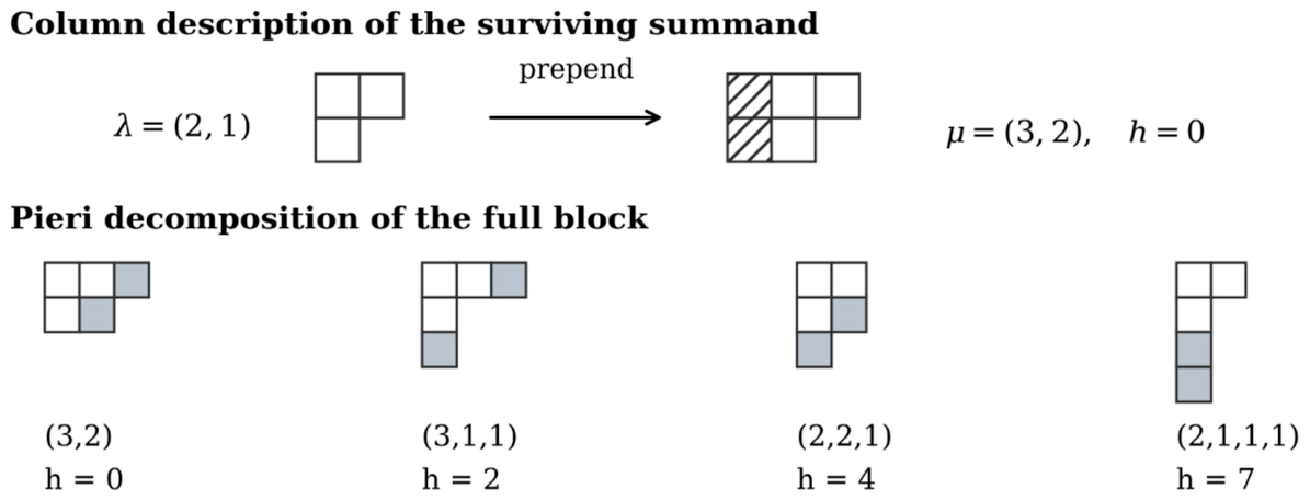
Figure 2.
(a) Generator dimensions for dimW = 3; blank cells are zero, and for p ≥ 2 the support lies in n ≥ 2p. (b) The multiplicities of 𝕊(n−2−j,j)W in ; outlined cells have n = 2j + 2 and multiplicity Catj+1 − 1. Shading increases with the logarithm of the value.
Figure 2.
(a) Generator dimensions for dimW = 3; blank cells are zero, and for p ≥ 2 the support lies in n ≥ 2p. (b) The multiplicities of 𝕊(n−2−j,j)W in ; outlined cells have n = 2j + 2 and multiplicity Catj+1 − 1. Shading increases with the logarithm of the value.
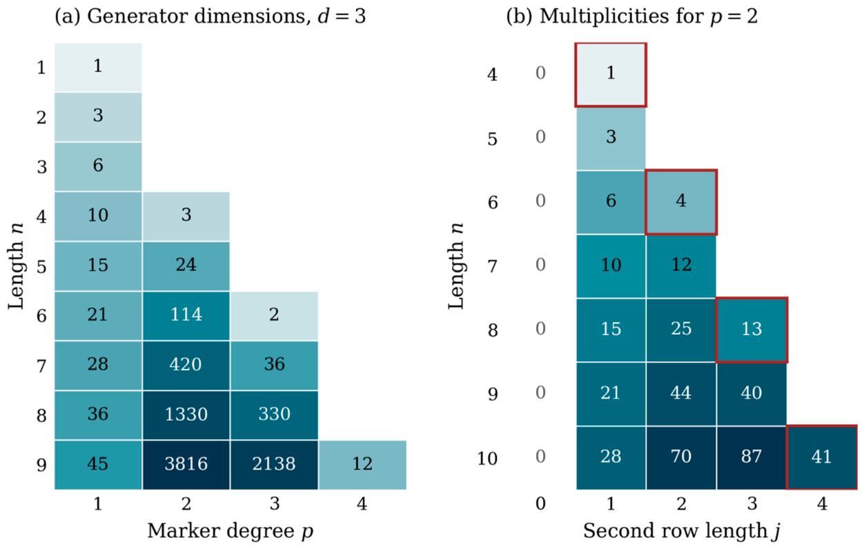
Figure 3.
Ext degree i = m − 1 − νm,n of bottom homology under Proposition 9.5. Integral bottom homology is torsion-free exactly where i ≤ 1 (Corollary 9.4); boxes mark n = 2m − 4 and n = 2m − 3.
Figure 3.
Ext degree i = m − 1 − νm,n of bottom homology under Proposition 9.5. Integral bottom homology is torsion-free exactly where i ≤ 1 (Corollary 9.4); boxes mark n = 2m − 4 and n = 2m − 3.
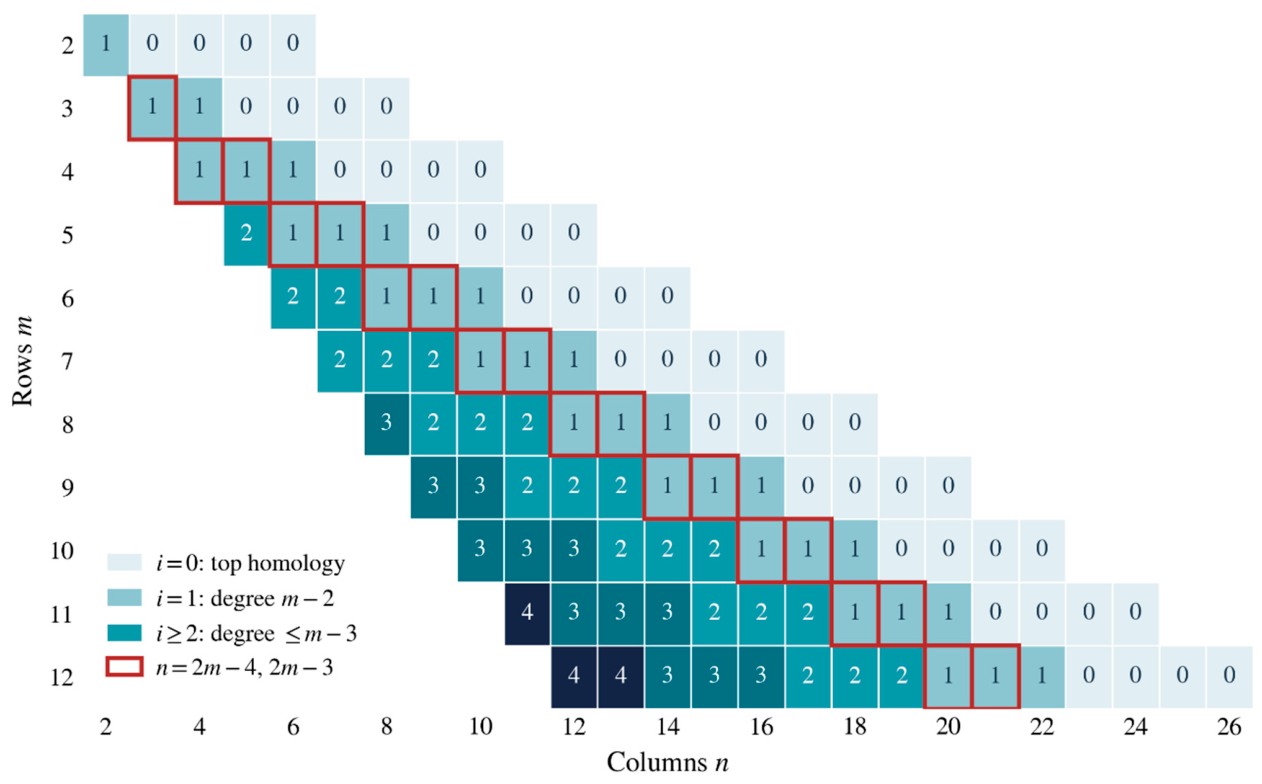

Table 1.
The ambient objects and the roles of their symmetries.
| Object | Definition or role | Acting symmetry |
| p odd markers and n − p ordinary slots | GL(W) × Sn | |
| dθ | Contraction with a fixed frame θ ∈ W* | Sn; generally not G |
| Kernel of every dϕ | GL(W) × Sn | |
| G-fixed cochains killed by dθ | Sn | |
| aλ | Group-dependent multiplicity |
Table 2.
First-column deletion at n = 5 and d = 3.
| μ | p = 𝓵(μ) | μ− | fμ | Contribution | |
| 5 | 1 | 4 | 1 | 15 | 15 |
| 4,1 | 2 | 3 | 4 | 10 | 40 |
| 3,2 | 2 | 2,1 | 5 | 8 | 40 |
| 3,1,1 | 3 | 2 | 6 | 6 | 36 |
| 2,2,1 | 3 | 1,1 | 5 | 3 | 15 |
| 2,1,1,1 | 4 | 1 | 4 | 3 | 12 |
| 1,1,1,1,1 | 5 | ∅ | 1 | 1 | 1 |
| Total | 159 |
Table 3.
The entire λ = (2,1) block at n = 5, p = 2.
| Total partition μ | dimSμ | hλ,μ | In the joint kernel? |
| 3,2 | 5 | 0 | Yes |
| 3,1,1 | 6 | 2 | No |
| 2,2,1 | 5 | 4 | No |
| 2,1,1,1 | 4 | 7 | No |
Table 4.
Single-frame and joint kernels on the full cochain space.
| n | p | d | dim kerdθ | ||
| 2 | 1 | 2 | 4 | 3 | 2 |
| 3 | 1 | 2 | 12 | 7 | 3 |
| 4 | 1 | 2 | 32 | 15 | 4 |
| 4 | 2 | 2 | 24 | 17 | 11 |
| 5 | 2 | 2 | 80 | 49 | 26 |
| 4 | 2 | 3 | 54 | 43 | 24 |
| 6 | 3 | 3 | 540 | 422 | 233 |
Table 5.
C2-invariant cochains in Example 8.2: the two frame kernels by exact rational row reduction, and the joint invariant kernel from (4.3).
Table 5.
C2-invariant cochains in Example 8.2: the two frame kernels by exact rational row reduction, and the joint invariant kernel from (4.3).
| (n,p) | θ+ (cyclic) | θ0(not cyclic) | ||
| (3,1) | 6 | 2 | 4 | 2 |
| (4,2) | 12 | 6 | 9 | 6 |
| (5,2) | 40 | 13 | 24 | 13 |
Table 6.
Rational ranks of the stacked contraction matrix. Each kernel dimension agrees with the Column Law.
Table 6.
Rational ranks of the stacked contraction matrix. Each kernel dimension agrees with the Column Law.
| n | p | d | Cochain dimension | Stacked rank | Kernel dimension |
| 2 | 1 | 2 | 4 | 2 | 2 |
| 3 | 1 | 2 | 12 | 9 | 3 |
| 3 | 2 | 2 | 6 | 2 | 4 |
| 4 | 1 | 2 | 32 | 28 | 4 |
| 4 | 2 | 2 | 24 | 13 | 11 |
| 4 | 3 | 2 | 8 | 2 | 6 |
| 5 | 2 | 2 | 80 | 54 | 26 |
| 5 | 3 | 2 | 40 | 17 | 23 |
| 4 | 2 | 3 | 54 | 30 | 24 |
| 6 | 3 | 2 | 160 | 88 | 72 |
| 5 | 2 | 3 | 270 | 190 | 80 |
| 5 | 3 | 3 | 90 | 39 | 51 |
| 6 | 2 | 3 | 1,215 | 975 | 240 |
| 4 | 2 | 4 | 96 | 54 | 42 |
| 6 | 3 | 3 | 540 | 307 | 233 |
Disclaimer/Publisher’s Note: The statements, opinions and data contained in all publications are solely those of the individual author(s) and contributor(s) and not of MDPI and/or the editor(s). MDPI and/or the editor(s) disclaim responsibility for any injury to people or property resulting from any ideas, methods, instructions or products referred to in the content. |
© 2026 by the authors. Licensee MDPI, Basel, Switzerland. This article is an open access article distributed under the terms and conditions of the Creative Commons Attribution (CC BY) license (http://creativecommons.org/licenses/by/4.0/).
Copyright: This open access article is published under a Creative Commons CC BY 4.0 license, which permit the free download, distribution, and reuse, provided that the author and preprint are cited in any reuse.