Stakeholder Pressure and Verification in the Low Carbon Transition

1. Introduction

Consider a manufacturer choosing among cleaner equipment, water-saving processes, and a sustainability communication campaign. Equipment and process improvements change genuine outcomes and may lower operating costs. Communication can change how stakeholders assess the firm. All three use resources that could otherwise support production. Customers, investors, or other stakeholders may reward a favorable assessment, so the firm’s response depends on what the assessment measures, how it is verified, and which benefits managers recognize. The model asks how these features shape investment in the low-carbon transition.

The model separates genuine carbon and non-carbon outcomes, a metric aggregating them, and the stakeholder assessment. The assessment combines verified metric performance with a soft component influenced by communication. The gap between these components explains verification’s immediate effect: it raises the assessment when verified performance is higher and lowers it when the soft component is higher. The firm then adjusts its activities. Metric weights introduce a separate issue, because a broad sustainability metric can improve largely through non-carbon outcomes.

Assessment-oriented effort can include framing, branding, outreach, or selective emphasis on truthful but nonverified information. It need not be deceptive. Research on greenwashing and selective disclosure motivates this channel (Delmas and Burbano, 2011; Marquis et al., 2016), but the model also permits truthful activity that changes the soft assessment component without changing genuine outcomes. Communication that becomes independently verified belongs to the verification margin. Stakeholder assessment is an institutional evaluation technology rather than a Bayesian posterior or a signaling equilibrium.

The first main result is that verification can reduce genuine investment (Proposition 1). Consider the manufacturer whose verified performance is stronger than its soft assessment component. Better verification raises its assessment at unchanged activities. When further assessment gains bring sufficiently smaller stakeholder rewards, this increase can weaken the incentive to invest more. That effect can outweigh the higher assessment weight on genuine performance, even while communication remains active. The reversal depends on how rapidly marginal stakeholder rewards diminish and the firm’s adjustment across activities; the gap’s sign alone is insufficient. Corollary 2 gives cleaner component signs when stakeholder rewards rise linearly with the assessment (affine rewards) and choices across activities can be analyzed separately (a separable allocation problem).

The second main result is a minimum verification requirement for implementation (Proposition 2). One scalar pressure instrument can support an interior socially optimal genuine allocation only if the metric gives the right relative incentives across activities, the metric congruity requirement in Lemma 2. Even with those weights, weak verification can make communication attractive at the pressure needed to induce genuine investment. The threshold identifies when that additional obstacle disappears.

The third main result is that genuine outcomes and assessment can move in opposite directions (Proposition 3). In this benchmark, with favorable governance channels, governance improves genuine outcomes or leaves them unchanged. If it strengthens verification, it can also remove weight from a favorable soft assessment component. The assessment can fall when genuine improvement does not offset that loss. A construction with governance acting only through verification establishes the possibility. It does not predict that governance generally lowers assessments.

A focused extension gives carbon its own verification margin (Section 4.11). For the manufacturer, an improvement in emissions assurance can change the reward for cleaner equipment without changing verification of water savings. The relative incentive depends on both metric weights and the ratio of verification qualities. Proposition 4 characterizes when that ratio supports the social target and when remaining rewards for communication prevent implementation. The three main propositions retain the common-verification baseline.

Supporting results distinguish operating performance from full firm payoff. Stakeholder payments enter the latter, while operating efficiency measures performance before those payments. Pressure can initially improve operating performance when managers underweight operating benefits and the induced investment response is suitably aligned with them. A later decline requires an additional condition. An operating-efficiency optimum need not maximize full firm payoff or welfare.

The analytical foundation is multitask incentive and performance-measurement theory, which explains why a misaligned measure distorts effort allocation (Holmström and Milgrom, 1991; Baker, 1992, 2002; Feltham and Xie, 1994). Lemma 2 applies that established congruity logic. The lemmas and corollaries supply allocation, targeting, and operating-performance benchmarks for the three main propositions. The model studies resource allocation after stakeholder rewards reach the firm, complementing theories of stakeholder pressure and sustainable investing.

A numerical illustration shows that several benchmark mechanisms can coexist. Governance raises genuine performance while lowering the assessment in one regime, favorable incentive alignment permits an initial efficiency gain from pressure, and a low carbon weight produces little decarbonization despite a broader metric improvement. These are illustrative patterns rather than empirical estimates. Section 7 retains the outcome comparison; Appendix C gives the parameterization, figures, derivations, and checks.

Section 2 positions the contribution in the literature. Section 3 states the model and assumptions; Appendix A supplies additional details and a managerial microfoundation. Section 4 and Section 5 derive the pressure, verification, welfare, and governance results, with proofs in Appendix B. Section 6 develops empirical and practical implications. Section 7 presents the numerical comparison, and Section 8 concludes.

2. Literature Review and Theoretical Positioning

2.1. Sustainability Outcomes and Their Assessment

Sustainability covers multiple environmental, economic, and social outcomes. Liu et al. (2017) document this breadth within social sustainability and the difficulties of consistent operationalization. Carbon-specific evidence is therefore necessary when studying the low-carbon transition. Bolton and Kacperczyk (2021) examine emissions and investor compensation for carbon risk; Azar et al. (2021) study institutional engagement and subsequent emissions; Flammer (2021) reports changes in both environmental ratings and emissions following green-bond issuance.

External assessments add a separate measurement layer. Berg et al. (2022) attribute ESG-rating divergence to differences in scope, measurement, and weighting, with measurement contributing the largest share. A stakeholder-facing rating may proxy an institutional assessment, whereas a genuine-performance metric requires explicit aggregation of underlying outcomes. Neither automatically measures decarbonization. The model maintains these distinctions rather than treating sustainability performance as one observable index.

2.2. Stakeholder Pressure and Corporate Response

Wang et al. (2020), in a meta-analysis of 58 studies, find an overall positive association between stakeholder pressures and environmental strategies, with variation across pressure types and settings. Their internal, coercive, market, and social categories identify different sources of corporate incentives. Dyck et al. (2019) associate institutional ownership with environmental and social performance, while Azar et al. (2021) document engagement concentrated among high-emitting firms and a negative association between large institutional ownership and subsequent emissions.

The measured response remains crucial. Wang et al. (2020) note that environmental management and environmental performance are sometimes conflated. A strategy or disclosure program need not improve physical outcomes. The model summarizes the value of a favorable assessment through stakeholder pressure and asks how that incentive is allocated among genuine and assessment-oriented activities.

2.3. Disclosure Greenwashing and Verification

Pineiro-Chousa et al. (2016) connect environmental performance, disclosure, and reputational-risk management. Delmas and Burbano (2011) examine the drivers of greenwashing; Lyon and Maxwell (2011) model strategic environmental disclosure under possible activist audit and penalties. Lyon and Montgomery (2015) synthesize the different forms of misleading environmental communication grouped under greenwash. Marquis, Toffel, and Zhou (2016) study selective disclosure and scrutiny, while Berrone, Fosfuri, and Gelabert (2017) show that apparent responsibility can backfire when actual performance deteriorates under substantial NGO scrutiny. These studies motivate a separate assessment channel. Here r also includes truthful nonverified communication, so positive assessment-oriented effort alone does not establish greenwashing.

Assurance and reporting institutions can strengthen the link to genuine performance. Simnett, Vanstraelen, and Chua (2009) find that firms seeking reporting credibility and a stronger reputation are more likely to obtain voluntary assurance. Christensen, Hail, and Leuz (2021) examine the informational and real effects of mandatory sustainability reporting; Flammer (2021) finds a stronger investor response to certified green bonds and subsequent changes in ratings and emissions. The model distinguishes the value attached to an assessment from the verification weight linking it to genuine metric performance.

Stakeholder payments may depend on a rating or eligibility score, allowing communication to affect rewards through that score before genuine outcomes change. Berg et al. (2022) document differences in rating scope, measurement, and weighting, motivating the treatment of assessment as a constructed measure.

The positive effect of r on its soft input is a separate modeling assumption. For example, an institutional rule that credits the presentation of an unverified initiative can reward communication without changing D or H. The firm responds to that rule, while independently verified communication belongs to the verification margin. The assessment is an institutional evaluation rule rather than a Bayesian posterior; endogenous stakeholder learning or redesign of the rule would require an additional model.

2.4. Corporate Governance

Castillo-Merino and Rodríguez-Pérez (2021) contrast agency and good-governance explanations and examine governance as a moderator of institutional influences on financial firms’ ESG performance. Ferrell, Liang, and Renneboog (2016) associate stronger governance and fewer agency concerns with greater CSR activity. Eccles, Ioannou, and Serafeim (2014) identify differences in board responsibility, incentives, engagement, and measurement among firms with long-standing sustainability policies. Because governance is itself included in many ESG indexes, using it to explain the same aggregate index can obscure the mechanism. Here governance enters structurally through managerial internalization, verification, implementation costs, and assessment-oriented effectiveness.

2.5. Sustainability and Corporate Operating Performance

Environmental investment consumes resources but may also improve the firm’s operating performance. Porter and van der Linde (1995) argue that well-designed environmental requirements can stimulate innovation and resource-productivity gains. Hart and Ahuja (1996) find that emission reductions can precede improved operating performance, particularly among initially high-emitting firms. Eccles et al. (2014) document organizational and long-term performance differences associated with sustainability policies. Gillan, Koch, and Starks (2021) emphasize competing explanations and unresolved empirical results in the ESG and CSR literature.

Castillo-Merino and Rodríguez-Pérez (2021) consider both agency costs and mutually reinforcing sustainability and financial performance. In reviewing earlier studies, Wang et al. (2020) discuss regulatory costs and evidence of non-monotonic environmental actions under government pressure. This motivates an analysis of when stakeholder incentives correct underinvestment in operating benefits and when they instead induce excessive genuine investment or assessment-oriented expenditure.

2.6. Economic Theory and the Research Gap

The closest analytical benchmark is multitask agency and performance measurement. Holmström and Milgrom (1991) show how incentives on measured tasks distort effort allocation. Baker (1992) studies measures that differ from the principal’s objective, Feltham and Xie (1994) formalize congruity, and Baker (2002) distinguishes measurement distortions from risk. Lemma 2 applies this established logic to the metric weights needed to support an interior genuine allocation. The additional implementation issue arises because stakeholder rewards depend partly on a separately manipulable assessment channel.

Theories of stakeholder pressure and corporate social responsibility explain why external concerns enter corporate decisions. Baron (2001) models activist pressure and separates profit-motivated responses from broader social objectives. Bénabou and Tirole (2010) discuss delegated prosocial preferences and long horizons; Hart and Zingales (2017) distinguish shareholder welfare from market value when investors value externalities. The present model takes the strength of stakeholder rewards as given and studies the composition of the firm’s response.

Sustainable-investing theory addresses how investor preferences reach firms. Heinkel, Kraus, and Zechner (2001) show how green-investor exclusion can raise polluting firms’ cost of capital enough to change technology. Pástor, Stambaugh, and Taylor (2021) analyze green preferences and climate hedging in general equilibrium; Oehmke and Opp (2025) study the roles of financing conditions and investment mandates in reducing externalities. This paper begins after these incentives reach the managerial objective, allowing similar pressure to originate with customers, employees, communities, or other stakeholders.

Disclosure and reputation models provide a further comparison. Fischer and Verrecchia (2000) analyze costly reporting bias when the market is uncertain about managerial objectives. Their model connects reporting incentives to the informativeness of a report. Lyon and Maxwell (2011) study strategic environmental disclosure under audit, while signaling, career-concern, and reputation models incorporate equilibrium inference about hidden information (Stein, 1989; Holmström, 1999). The present model takes the institutional assessment mapping as given and asks how rewards under that mapping allocate resources between genuine outcomes and assessment-oriented activity.

The three main propositions isolate mechanisms generated by separating the metric from assessment: verification-curvature reversal (Proposition 1), a verification threshold for first-best implementation despite metric congruity (Proposition 2), and governance-induced divergence between genuine outcomes and assessment within the benchmark (Proposition 3). Supporting lemmas and corollaries establish the allocation and targeting benchmarks and the conditions under which pressure locally corrects managerial underinvestment in operating benefits. The contribution concerns institutional assessment interacting with corporate resource allocation. Section 4.11 extends the linear metric to separate carbon and non-carbon verification, showing how assurance scope changes targeting across genuine outcomes.

3. Model

3.1. Activities Outcomes and Stakeholder Assessment

A firm allocates a fixed organizational resource base M>0 among production and three nonnegative activities: decarbonization effort d, other genuine sustainability effort h, and assessment-oriented effort r. Genuine outcomes are D=D(d) and H=H(h), with positive and weakly decreasing marginal products. D is explicitly a carbon outcome; H captures the other substantive sustainability outcome. A jointly concave metric S(D,H), increasing in both arguments, aggregates them. Its weights need not equal their social values.

Stakeholders respond to an institutional assessment that combines verified metric performance with a soft component:

Ŝ = θS(D,H) + (1 - θ)[S̄ + R(r)].

Here θ∈[0,1] is verification quality, S̄ is the soft-component baseline, and R is increasing and concave. The activity r changes this component while holding genuine outcomes and verification fixed; it can include truthful framing or outreach. Independently verified communication belongs to θ. When θ=1, the assessment equals S and r has no direct assessment effect. This is a reduced-form evaluation technology, not a Bayesian posterior. For z=(d,h,r), define the verified-versus-soft gap

Δ(z) = S(D,H) − [S̄ + R(r)].

For illustration, hold activities fixed and measure both components on the same scale. If verified performance is 8 and the soft component is 4, raising θ from 0.25 to 0.75 raises the assessment from 5 to 7. Reversing the component values lowers it from 7 to 5. These are arithmetic examples, not predicted equilibrium responses. The gap describes assessment components; its sign alone establishes neither deception nor deliberate undercommunication. Appendix A.4 gives further outcome and optimality details.

3.2. Resources and Corporate Incentives

Resource costs are C_D(d), C_H(h), and C_R(r). Remaining resources produce ordinary output F(x), where

x = M - C_D(d) - C_H(h) - C_R(r),

The resource constraint is x≥0. Genuine activities also generate operating benefits A_D(d) and A_H(h) accruing to the firm. Corporate operating efficiency, meaning real operating performance before assessment-contingent stakeholder payments, is

$ℰ$(d,h,r) = F(x) + A_D(d) + A_H(h).

This measures real operating performance from the fixed resource base, rather than technical efficiency in the production-theory sense. Assessment-oriented effort has no direct operating benefit in the baseline. All payoff components are expressed in common units. Stakeholder pressure λ≥0 scales the assessment-contingent net pecuniary payment T(z;λ)=λB(Ŝ(z)) received by the firm. B is increasing and concave; its level may represent a net reward or penalty. The full firm payoff is

Π(z;λ) = $ℰ$(z) + T(z;λ) = $ℰ$(z) + λB(Ŝ(z)).

The managerial objective is

V(d,h,r) = F(x) + ω[A_D(d) + A_H(h)] + λB(Ŝ).

over the feasible set

$𝒳$ = {(d,h,r) ∈ ℝ₊³ : C_D(d) + C_H(h) + C_R(r) ≤ M}.

Managers attach weight ω∈(0,1] to genuine operating benefits: ω=1 represents full internalization, while ω<1 captures short horizons or other organizational frictions. At ω=1, V equals the full firm payoff Π; otherwise V underweights operating benefits while retaining the stakeholder payment. Demand, financing, employment, or reputational channels motivate these payments, but the baseline represents their pecuniary transfer component only. Any associated productivity gains, consumer utility, information benefits, or financing efficiencies beyond transfers would require additional operating or welfare terms. The parameters λ, θ, and ω describe incentive strength, verification, and managerial internalization. Appendix A.1 gives a two-period microfoundation; Appendix A.4 gives the marginal incentives and complementary-slackness conditions. Activities may optimally be zero.

3.3. Maintained Conditions

Primitives are continuous on feasible domains and twice continuously differentiable on relevant interiors when derivatives are used. The following assumptions govern the general model; Appendix A.5 explains their role in uniqueness and differentiation. Governance-specific conditions appear in Section 5.1.

Assumption 1 (Resource costs). For j ∈ {D,H,R}, C_j(0)=0, C_j′>0, C_j″≥0, and resource costs are coercive, meaning that they grow without bound as activity rises.

Assumption 2 (Technology and operating benefits). F is increasing and strictly concave, with marginal productivity becoming large as productive resources approach zero. This boundary condition keeps production active by making the last resources retained for production especially valuable. The functions A_D, A_H, D, H, and R are concave on the relevant domains, with A_D′≥0 and A_H′≥0. The right derivative of the assessment technology at the origin exists and is finite: 0<R′(0)<∞.

Assumption 3 (Sustainability and stakeholder response). S(D,H) is jointly concave and increasing in both arguments, while B(Ŝ) is increasing and concave.

Assumption 4 (Strict resource-cost curvature for uniqueness). For general-model results that invoke a unique optimizer or differentiable comparative statics, C_j″>0 for j∈{D,H,R} on the relevant domain. Together with Assumptions 1–3, this makes the production-resource term strictly concave and the interior Hessian of V negative definite. For results explicitly invoking the affine-separable benchmark, the one-dimensional strict-concavity conditions in Assumption 5 replace this requirement.

Differentiable comparative statics hold the active set fixed locally. Boundary choices are treated through the separate Kuhn–Tucker or monotone-comparative-static arguments. Proofs are in Appendix B.

3.4. The Affine Separable Benchmark

Sharper signed responses use the following benchmark, which removes stakeholder-value curvature and interactions through nonlinear productive output or a binding resource constraint.

Assumption 5 (Affine-separable benchmark). In results explicitly invoking the benchmark, F(x)=νx with ν>0, S=α_mD+β_mH with α_m,β_m>0, and B(Ŝ)=b₀+b₁Ŝ with b₁>0. The strict-concavity and boundary conditions imposed on F in Assumption 2 do not apply. The common resource constraint is slack at the relevant optimum, and each one-dimensional component problem is strictly concave.

Slackness is maintained throughout the parameter region under consideration. The objective then separates into three strictly concave component problems, given in Appendix A.6. This benchmark replaces the relevant general-model restrictions; it is not an additional restriction requiring F to be both strictly concave and linear. Results relying on it explicitly invoke Assumption 5. Section 4.11 states explicitly how the benchmark changes when verification differs across outcomes.

3.5. Analytical and Numerical Methods

The analysis derives constrained optimality conditions and comparative statics from the stated primitives; formal proofs appear in Appendix B. The numerical illustration evaluates the specified component choices and operating-performance formulas using illustrative parameters reported in Appendix C. ChatGPT assisted with drafting and revision, literature organization, alternative theoretical formulations, algebraic and logical consistency checks, and numerical checking and figure preparation through executable calculations. The numerical results were computed from the stated formulas. Details of the tool used and author responsibility are disclosed in the Acknowledgments.

4. Social Pressure, Verification, and Corporate Responses

This section examines how the firm responds to changes in stakeholder pressure and environmental verification. The analysis first establishes results that hold in the general model and then uses the separable benchmark of Section 3.4 to obtain sharper directional predictions. The final subsections introduce social welfare and show why credible verification, although important, is not by itself sufficient to generate the socially preferred allocation of sustainability effort.

The full technical statements, including boundary cases and proofs, are collected in Appendix B. The main text emphasizes the economic content of the results.

4.1. Existence and the Basic Corporate Choice

Under Assumptions 1–3, the firm’s feasible set is compact and its objective is continuous and concave. An optimal allocation therefore exists. Under Assumption 4, the production-resource component is strictly concave and the remaining terms are concave, so the full objective is strictly concave and the optimal allocation

z* = (d*, h*, r*)

is unique and varies continuously with the model parameters.

This preliminary result is useful because the three activities need not all be positive. A firm may undertake no assessment-oriented activity when verification is sufficiently strong, or it may choose zero activity in one genuine sustainability dimension when its marginal benefit is too small. The subsequent results therefore do not depend on assuming an interior solution unless this is explicitly stated.

A particularly simple implication concerns assessment-oriented activity. If there is no stakeholder pressure,

λ = 0,

then

r* = 0,

because assessment-oriented expenditure consumes resources without producing either a genuine sustainability outcome or a direct operating benefit. The same conclusion holds under perfect verification,

θ = 1,

because assessment-oriented activity no longer affects stakeholder assessments.

When λ > 0 and θ < 1, however, r* > 0 can be optimal. The firm compares the marginal stakeholder benefit of raising the soft assessment component with the marginal resource cost of doing so. Thus imperfect verification can create an economic return to assessment-oriented activity even when the firm makes no false statements.

4.2. What Stronger Social Pressure Guarantees

A central question is whether stronger stakeholder pressure necessarily produces better environmental outcomes. The general model gives a strong answer for the stakeholder sustainability assessment but a deliberately weaker answer for the genuine-sustainability performance metric.

Let

P(z) = B(Ŝ(z))

denote the assessment-contingent payment per unit of pressure, and let

Gω(z) = F(x) + ω[A_D(d) + A_H(h)]

denote the part of the managerial objective that would remain in the absence of stakeholder pressure.

Consider two levels of pressure,

λ₂ > λ₁.

The optimality of the firm’s choices at the two values of λ implies the following result.

Lemma 1. Social pressure weakly increases the stakeholder sustainability assessment. Holding verification and managerial internalization fixed, stronger stakeholder pressure weakly increases the firm’s optimal assessment.

Ŝ*(λ₂) ≥ Ŝ*(λ₁).

At the same time,

Gω[z*(λ₂)] ≤ Gω[z*(λ₁)].

More precisely,

λ₁(P₂ − P₁) ≤ Gω,1 − Gω,2 ≤ λ₂(P₂ − P₁).

The first conclusion is general: stronger pressure makes the firm choose an allocation that generates at least as much stakeholder-valued assessment.

What does not follow is equally important. Lemma 1 does not imply

D*(λ₂) ≥ D*(λ₁)

or even

S*(λ₂) ≥ S*(λ₁).

The firm is rewarded for the stakeholder sustainability assessment, not directly for either decarbonization or the genuine-sustainability performance metric. When verification is imperfect, it can respond through genuine decarbonization, other genuine sustainability activity, assessment-oriented activity, or a combination of the three.

This distinction provides a theoretical explanation for why greater stakeholder attention to sustainability can produce a change in reporting or reputation through the soft assessment channel without an equally strong change in underlying emissions.

4.3. Social Pressure and Corporate Operating Efficiency

Pressure can improve operating performance by correcting benefits that managers initially underweight. With full internalization, that correction is absent: at zero pressure the firm already maximizes $ℰ$, and further pressure cannot raise it.

Corollary 1. Social pressure cannot improve operating efficiency in the frictionless benchmark. If ω = 1 and λ₂ > λ₁, then

$ℰ$[z*(λ₂)] ≤ $ℰ$[z*(λ₁)].

Under uniqueness, the inequality is strict whenever the firm’s optimal allocation changes.

Corollary 1 concerns operating performance before stakeholder payments. It does not establish a decline in the full firm payoff Π; at ω=1 managers maximize that payoff, including payments, at each pressure level.

When ω<1, pressure can instead encourage investments whose operating benefits managers underweight. Consider a unique interior optimum in the two genuine activities at zero pressure, with assessment-oriented effort remaining at zero for small pressure increases and a negative-definite Hessian on the genuine margins. A small increase in pressure improves $ℰ$ if the induced investment response has a positive combined contribution to the omitted operating benefits. Write Γθ for the sum of each genuine activity’s marginal operating benefit multiplied by that activity’s local response to pressure at zero pressure. The condition Γθ>0 requires this combined contribution to be positive after accounting for interactions between activities; agreement in the signs of their separate marginal benefits is insufficient. Appendix B.3 gives the formal expression and derivation. With no verification, this first-order correction through genuine activity vanishes.

An initial gain need not persist as pressure rises. If every assessment-maximizing allocation yields lower operating performance than the zero-pressure allocation, sufficiently strong pressure eventually reverses the gain. Together with the local alignment, uniqueness, and continuity conditions, this yields a finite positive operating-efficiency-maximizing pressure λᴱ. Appendix B.3 states the exact condition and proof. A globally single-peaked inverted-U does not follow, and λᴱ need not maximize full firm payoff or welfare.

4.4. Verification and Diminishing Stakeholder Rewards

Verification changes how performance translates into an assessment. The resulting change in marginal stakeholder rewards explains why better verification need not produce more genuine investment.

Use the gap Δ defined in Section 3.1. At unchanged activities, a positive gap means verification raises the assessment; a negative gap means it lowers it. With diminishing marginal rewards, the first change reduces the payment earned from an additional assessment gain, while the second increases it. Both occur alongside verification’s direct shift in assessment weight toward genuine performance. The balance between these effects, followed by the firm’s adjustment, determines investment.

Define the marginal stakeholder returns to the three activities as

J_D = λB′(Ŝ)θS_DD′,

J_H = λB′(Ŝ)θS_HH′,

and

J_R = λB′(Ŝ)(1 − θ)R′.

Measure the curvature of stakeholder rewards by

η_B(Ŝ) = −B″(Ŝ)/B′(Ŝ) ≥ 0.

For λ > 0, holding the activity vector fixed and taking 0 < θ < 1, the relative-return ratios are

J_D/J_R = [θ/(1 − θ)]·[S_DD′/R′]

and

J_H/J_R = [θ/(1 − θ)]·[S_HH′/R′].

Both ratios increase strictly with θ. This relative reweighting is robust to the curvature of B because the common factor B′(Ŝ) cancels.

For the carbon margin, the absolute marginal stakeholder return changes as follows at unchanged activities; Appendix B.4 gives the corresponding expressions for the other margins:

∂J_D/∂θ = λB′(Ŝ)S_DD′[1 − θη_B(Ŝ)Δ(z)].

The term 1 captures verification’s direct increase in the genuine-performance weight. The term θη_BΔ captures the change in marginal rewards caused by the assessment change. A positive gap permits the latter to outweigh the former, but the direct return falls only when θη_BΔ>1. Equilibrium investment also responds to resource costs and adjustment in other activities. In the statement below, a zero-activity (corner) solution means that the firm chooses none of that activity.

Proposition 1. Verification has an unambiguous relative effect but an ambiguous absolute effect. For λ > 0 and 0 < θ < 1, better verification strictly raises J_D/J_R and J_H/J_R holding the activity vector fixed. With concave stakeholder valuation, however, the absolute marginal returns J_D, J_H, and J_R need not move in the corresponding directions. In a one-genuine-margin local corner case with h*=r*=0 and d*>0, provided those corners remain unchanged for the local perturbation, sign(∂d*/∂θ)=sign[1−θη_B(Ŝ*)Δ*]. More strongly, the reversal can occur while assessment-oriented activity remains active: admissible primitives exist with d*>0, r*>0, and ∂d*/∂θ<0.

The scalar sign formula in Proposition 1 applies when the other activities remain at their corners. When communication adjusts, its response can offset the direct incentive to cut genuine investment, so stronger curvature may be needed. Appendix B.4 gives the exact interior condition and a construction with d*=1 and r*=0.1 in which better verification locally reduces both activities. Thus the reversal can occur with active communication; neither a positive gap nor diminishing rewards alone guarantees it.

If stakeholder valuation is affine, η_B = 0 and this curvature channel disappears. The next subsection shows that the familiar positive verification signs then emerge under the affine-separable benchmark.

4.5. Verification in the Affine Separable Benchmark

Suppose stakeholder valuation is affine:

B(Ŝ) = b₀ + b₁Ŝ, b₁ > 0.

With affine rewards, η_B=0: verification increases the direct marginal stakeholder return to genuine activity and reduces it for assessment-oriented effort. It also gives a general composition result using the gap Δ from Section 3.1:

For θ₂ > θ₁, revealed preference implies

Δ[z*(θ₂)] ≥ Δ[z*(θ₁)].

Thus better verification weakly increases the verified-performance component relative to the soft assessment component even when the common resource constraint can bind.

Under the affine-separable benchmark of Assumption 5, the individual activity responses can also be signed. For the corresponding interior component choices, define

K_D = νC_D″ − ωA_D″ − λb₁θα_mD″ > 0, K_H = νC_H″ − ωA_H″ − λb₁θβ_mH″ > 0, K_R = νC_R″ − λb₁(1 − θ)R″ > 0.

For λ > 0, implicit differentiation gives

∂d*/∂θ = λb₁α_mD′/K_D > 0,

∂h*/∂θ = λb₁β_mH′/K_H > 0,

and

∂r*/∂θ = −λb₁R′/K_R < 0.

At corners, the corresponding verification responses are weak: ∂d*/∂θ ≥ 0, ∂h*/∂θ ≥ 0, and ∂r*/∂θ ≤ 0. The strict signs apply to the corresponding interior choices when λ > 0.

Stronger social pressure produces a different pattern. For 0 < θ < 1 and corresponding interior choices,

∂d*/∂λ = b₁θα_mD′/K_D > 0,

∂h*/∂λ = b₁θβ_mH′/K_H > 0,

and

∂r*/∂λ = b₁(1 − θ)R′/K_R > 0.

At corners, the corresponding pressure responses are weakly nonnegative.

Corollary 2. Affine valuation signs the assessment-component gap; separability signs individual activities. With affine B, better verification weakly increases Δ[z*(θ)] in the general model. Under Assumption 5, for λ > 0 it weakly increases d and h and weakly reduces r, while for 0 < θ < 1 stronger stakeholder pressure weakly expands all three response channels. The corresponding benchmark signs are strict for interior choices.

Affine rewards sign the gap’s response even with a binding common resource constraint. Signing each activity additionally requires separability. This distinction separates the benchmark from Proposition 1’s general-model reversal. The next subsections ask whether these incentives can implement a socially preferred allocation.

4.6. Metric Weights and Decarbonization

Even when verification succeeds in directing resources toward genuine activity, an improvement in the broad sustainability performance metric need not translate proportionately into lower carbon emissions.

Under the linear benchmark

S = α_mD + β_mH,

the response of the genuine-sustainability performance metric to any parameter τ is

dS*/dτ = α_mD′(d*)·∂d*/∂τ + β_mH′(h*)·∂h*/∂τ.

A positive change in S* therefore does not imply that the carbon contribution is large. Under Assumption 5, holding the other primitives fixed and maintaining local component curvature bounded away from zero, the direct decarbonization response to improved verification converges to zero as α_m approaches zero, while S can continue to rise through h.

Verification changes the assessment weight placed on the genuine-performance metric relative to the soft component. Perfect verification makes Ŝ coincide with S, but it does not determine how the metric divides weight between carbon and non-carbon outcomes. If the policy objective is specifically a low-carbon transition, carbon performance must therefore remain visible as a separate target.

4.7. Social Welfare

Corporate operating efficiency does not capture all of the benefits produced by genuine sustainability activity. Decarbonization reduces climate damages, while non-carbon sustainability activity may generate other environmental or social benefits that are not fully captured by the firm.

Let Φ_D(D) denote the external social benefit of decarbonization and Φ_H(H) the external benefit associated with other genuine sustainability outcomes, with both increasing and concave.

Social welfare is

W(d,h,r) = $ℰ$(d,h,r) + Φ_D[D(d)] + Φ_H[H(h)].

The welfare population includes the firm and the stakeholders making or receiving T=λB(Ŝ). Their payment −T offsets the firm’s receipt +T, so the transfer cancels from aggregate welfare. Genuine external benefits enter through Φ_D and Φ_H. The assessment has no independent utility value in this baseline, and r has no direct operating or external benefit. Thus W includes $ℰ$ before payments, whereas the full firm payoff Π includes them. Treating stakeholder rewards as new resource surplus or adding direct benefits of communication would require a different welfare specification.

Since r consumes resources without producing either a genuine sustainability outcome or a direct external benefit,

r^FB = 0

at the first-best allocation. For an interior first best, genuine activity satisfies

F′(x^FB)C_D′(d^FB) = A_D′(d^FB) + Φ_D′(D^FB)D′(d^FB),

and

F′(x^FB)C_H′(h^FB) = A_H′(h^FB) + Φ_H′(H^FB)H′(h^FB).

These conditions make clear why the corporate optimum and social optimum need not coincide. The firm may underweight private operating benefits when ω < 1, and it does not directly internalize the external benefits Φ_D and Φ_H.

4.8. Perfect Verification Does Not Guarantee the First Best

Proposition 1 and Corollary 2 concern how information quality changes private incentives. The implementation problem is stricter: even if verification eliminates the soft assessment channel entirely, the sustainability performance metric may still reward the wrong mix of genuine activities.

Suppose verification is perfect:

θ = 1.

Assessment-oriented activity disappears, and stakeholder pressure operates only through the genuine-sustainability performance metric. It might therefore appear that sufficiently strong stakeholder pressure can always reproduce the social optimum. This is not generally true.

For an interior first-best genuine allocation, define the required incentive per marginal unit of the sustainability performance metric for decarbonization as

κ_D^FB = [(1 − ω)A_D′(d^FB) + Φ_D′(D^FB)D′(d^FB)] / [S_D^FBD′(d^FB)],

and for non-carbon sustainability as

κ_H^FB = [(1 − ω)A_H′(h^FB) + Φ_H′(H^FB)H′(h^FB)] / [S_H^FBH′(h^FB)].

Lemma 2. Perfect verification aligns assessment with the metric; first-best implementation also requires metric congruity. For an interior first-best genuine allocation, a single level of stakeholder pressure can decentralize the first-best allocation under perfect verification if and only if

κ_D^FB = κ_H^FB.

When the common value is κ^FB,

λ^FB = κ^FB / B′(S^FB).

The equality is the performance-measure congruity requirement from multitask agency theory (Holmström and Milgrom, 1991; Baker, 1992, 2002; Feltham and Xie, 1994). A single scalar incentive supports the desired allocation only when the metric supplies the right relative rewards across genuine activities. Lemma 2 is the targeting benchmark for the verification threshold in Proposition 2.

For the manufacturer, a metric heavily weighting water savings can make the pressure needed to induce the desired water investment too weak for the desired carbon investment. Increasing common verification does not repair that imbalance. Even with appropriate weights, however, insufficient verification can reward communication alongside genuine activity; Proposition 2 addresses this separate constraint.

For the linear performance-metric benchmark, S = α_mD + β_mH, the alignment condition becomes

[(1 − ω)A_D′/D′ + Φ_D′]/α_m = [(1 − ω)A_H′/H′ + Φ_H′]/β_m,

evaluated at the first-best allocation. The metric carbon weight α_m therefore matters independently of verification quality.

4.9. A Minimum Verification Requirement

When verification is imperfect, implementing the first best becomes more demanding because the level of stakeholder pressure required to support genuine activity may simultaneously make assessment-oriented activity profitable.

Normalize

R(0) = 0

Maintain the interior first-best genuine allocation and suppose the alignment condition of Lemma 2 holds. Let the common required genuine-activity incentive be κ^FB.

To support the first-best allocation while maintaining r^FB = 0, the marginal return to assessment-oriented activity at zero must not exceed its marginal resource cost. This requires

κ^FB[(1 − θ)/θ]R′(0) ≤ F′(x^FB)C_R′(0).

Solving for verification quality yields

θ̲ = κ^FBR′(0) / [κ^FBR′(0) + F′(x^FB)C_R′(0)].

Proposition 2. Conditional on metric congruity, first-best implementation requires sufficient verification. Under the interior first-best and targeting conditions of Lemma 2, the first-best allocation can be decentralized without assessment-oriented activity if and only if

θ ≥ θ̲.

Below the threshold, pressure supporting the desired genuine allocation also makes assessment-oriented activity attractive. At or above it, that pressure satisfies the zero-effort condition for r. Better targeting solves the relative-incentive problem across genuine activities; sufficient verification prevents the additional soft-channel response.

With common verification, congruity remains a prerequisite: if the genuine margins require different corrections per unit of the metric, no verification level makes one scalar pressure implement the first best. For κ^FB>0, the maintained positive marginal technology and cost terms imply 0<θ̲<1. The degenerate case κ^FB=0 requires both the external marginal benefit and the underinternalized operating-benefit term to vanish on each genuine margin; no corrective pressure is then needed and θ̲=0. The curvature and scale of B cancel from the threshold once pressure is chosen to support the congruent genuine margins.

4.10. Verification and Welfare

The welfare effect of better verification is not unconditional. If genuine sustainability activity is already above its socially preferred level, redirecting still more corporate resources toward it need not increase welfare.

The separable benchmark provides a transparent sufficient condition. Define

Ω_D = (1 − ω)A_D′ + [Φ_D′ − λb₁θα_m]D′

and

Ω_H = (1 − ω)A_H′ + [Φ_H′ − λb₁θβ_m]H′.

These terms measure the remaining social gain from additional genuine decarbonization and other sustainability effort after accounting for the stakeholder incentive already faced by the firm.

Verification and welfare result. Under Assumption 5, at any parameter value at which the unique optimizer is locally differentiable in θ, if

Ω_D ≥ 0, Ω_H ≥ 0,

then

dW*/dθ ≥ 0,

with a strict welfare improvement only when at least one contribution is strictly positive: Ω_D(∂d*/∂θ) > 0, Ω_H(∂h*/∂θ) > 0, or −νC_R′(∂r*/∂θ) > 0.

The condition requires additional genuine activity to remain socially valuable. In the separable benchmark, verification also reduces assessment-oriented expenditure, a resource cost with no direct welfare benefit. A strict welfare gain requires at least one strictly positive contribution.

Stakeholder pressure, verification, and metric design affect distinct incentive margins. Pressure raises the value to the firm of a favorable stakeholder assessment. Verification changes the relative assessment weights on genuine metric performance and the soft component, with equilibrium genuine-activity responses depending on the stated conditions. Metric design determines the relative rewards assigned to decarbonization and other genuine outcomes.

4.11. Carbon and Non Carbon Verification

An emissions assurance improvement can differ from verification of water savings or other non-carbon outcomes. Proposition numbers follow the contribution hierarchy: this extension is Proposition 4, while the governance result, Proposition 3, follows in Section 5.3. To examine that asymmetry, retain S=α_mD+β_mH with positive weights and replace common verification by θ_D,θ_H∈[0,1]. Let the outcome components share the existing communication activity r:

Ŝ₂ = α_m[θ_D D + (1 − θ_D)(D̄ + ℓ_D R(r))] + β_m[θ_H H + (1 − θ_H)(H̄ + ℓ_H R(r))].

(1)

The fixed soft baselines satisfy α_mD̄+β_mH̄=S̄. The nonnegative communication loadings satisfy α_mℓ_D+β_mℓ_H=1, and R(0)=0. Setting θ_D=θ_H=θ recovers the baseline assessment exactly. Costs, operating benefits, the managerial objective, and welfare retain their definitions, with Ŝ₂ replacing Ŝ in stakeholder payments. This extension allows verification to differ; it does not assume that carbon is always more verifiable.

At unchanged activities and with λ>0 and θ_D,θ_H>0, the ratio of marginal stakeholder returns to genuine activities is

J_D/J_H = (α_mθ_D D′)/(β_mθ_H H′).

(2)

The common marginal reward B′ cancels. Carbon verification therefore raises the relative reward for decarbonization even with concave rewards. Absolute investment responses still depend on reward curvature and resource competition. In the affine-separable benchmark of Assumption 5, with (1) replacing its common-verification assessment and slackness maintained over the comparison, raising θ_D at fixed θ_H weakly raises d, leaves h unchanged, and weakly lowers r. The carbon response is strict at an interior choice when λ>0 and local component curvature is positive. Appendix B.13 supplies the derivatives and the concave-reward qualification.

Proposition 2 asked whether one common verification level suffices. With two rates, targeting and the communication constraint become linked conditions on a verification pair. Evaluate κ_D^FB and κ_H^FB from Section 4.8 using S_D=α_m and S_H=β_m. Assume both corrections are positive and the first-best target has d^FB,h^FB,x^FB>0. Define

σ(θ_D,θ_H) = α_m(1 − θ_D)ℓ_D + β_m(1 − θ_H)ℓ_H,

K^FB = F′(x^FB)C_R′(0).

Proposition 4. Different verification rates change targeting and constrain implementation. For assessment (1), under Assumptions 1–4 with the linear metric, or the modified affine-separable benchmark at a slack first-best target, the target can be decentralized by one scalar pressure λ if and only if there exists t>0 such that

κ_D^FB/θ_D = κ_H^FB/θ_H = t, tσ(θ_D,θ_H)R′(0) ≤ K^FB.

(3)

Here θ_D,θ_H>0 and the implementing pressure is λ=t/B′(Ŝ₂^FB). The first equality matches the corrections needed on the two genuine margins. The inequality prevents communication from being profitable at zero. Define κ_L=α_mℓ_Dκ_D^FB+β_mℓ_Hκ_H^FB and κ_max=max{κ_D^FB,κ_H^FB}. The admissible verification pairs are exactly

(θ_D,θ_H) = (κ_D^FB/t, κ_H^FB/t), κ_max ≤ t ≤ κ_L + K^FB/R′(0).

(4)

Thus a pair exists precisely when K^FB≥R′(0)(κ_max−κ_L). With equal corrections and common verification, (3) reduces to Proposition 2’s threshold. With unequal corrections, the verification ratio can offset a targeting imbalance, but doing so leaves a soft channel that may prevent implementation. These are linked conditions on the pair, rather than independent minimum verification levels.

For example, Appendix B.13 gives a firm with κ_D^FB=2, κ_H^FB=1, equal communication weights, R′(0)=1, and K^FB=0.75. Carbon verification θ_D=1 and non-carbon verification θ_H=0.5 implement its target. If K^FB falls to 0.4, no verification pair can do so. More carbon assurance can therefore repair relative incentives without being sufficient to remove the communication obstacle.

5. Corporate Governance as a Structural Determinant of Sustainability Response

The governance analysis returns to the common-verification baseline. The preceding analysis treats managerial internalization and verification quality as characteristics of the firm’s decision environment. Corporate governance provides one institutional mechanism through which these characteristics can differ across firms.

Governance enters through managerial incentives, verification, and implementation technologies. It is a determinant of sustainability outcomes in this model.

Let

γ ∈ [0,1]

denote governance quality, with higher values representing stronger governance arrangements. Governance may include board oversight, managerial incentives, internal control systems, organizational accountability, sustainability expertise, and other mechanisms that affect corporate decision making.

The model allows governance to operate through four channels: managerial internalization, verification, implementation costs, and the effectiveness of assessment-oriented activity. The governance functions introduced below are assumed continuously differentiable to the order required by the comparative statics; where second cross-partials are used, they are assumed to exist and be continuous on the relevant domain.

5.1. Four Governance Channels

Managerial internalization. Governance can increase the extent to which managers recognize the long-run private operating benefits generated by genuine sustainability activity. Let

ω = ω(γ), ω′(γ) ≥ 0.

Better governance therefore moves managerial incentives closer to the firm’s long-run operating interests. This channel can represent longer managerial horizons, compensation systems that reward long-term performance, stronger board oversight, or internal decision processes that reduce managerial short-termism. When ω(γ) = 1, the managerial distortion associated with underweighting private sustainability benefits disappears.

Verification. Governance can also improve the quality of internal measurement, reporting, and control systems. To distinguish this channel from external verification, let v represent the quality of the external verification environment and write total verification quality as

θ = Θ(v,γ),

where

Θ_v > 0, Θ_γ ≥ 0.

External assurance, regulation, auditing standards, certification, and stakeholder monitoring can increase v. Internal controls, board oversight, environmental data systems, and governance quality can increase the governance component.

The stakeholder sustainability assessment becomes

Ŝ = Θ(v,γ)S(D,H) + [1 − Θ(v,γ)][S̄ + R(r;γ)].

This formulation distinguishes the external verification environment v from governance’s contribution to the institutional link between metric performance and stakeholder assessment.

Implementation costs. Better governance can reduce the organizational cost of genuine sustainability activity. Firms with effective internal coordination, stronger management systems, clearer accountability, and better access to relevant information may be able to implement decarbonization or other sustainability initiatives at lower cost.

Write

C_D = C_D(d;γ), C_H = C_H(h;γ),

and assume

∂C_D/∂γ ≤ 0, ∂C_H/∂γ ≤ 0.

More specifically, governance can reduce marginal implementation costs:

∂²C_D/(∂d∂γ) ≤ 0, ∂²C_H/(∂h∂γ) ≤ 0.

These conditions do not imply that governance makes sustainability investment costless. They simply allow better-governed firms to implement the same genuine activity with less organizational friction.

Assessment-oriented effectiveness. Finally, governance can reduce the effectiveness of activity that raises the soft assessment component without improving genuine outcomes. Let

R = R(r;γ)

and assume

∂²R/(∂r∂γ) ≤ 0.

For a given amount of assessment-oriented activity, stronger governance therefore weakens its marginal ability to influence the stakeholder assessment. One interpretation is that stronger internal controls, board oversight, and more credible reporting systems make it harder for soft communication to substitute for demonstrable performance. Another is that firms with stronger governance rely less heavily on symbolic responses because internal decision systems place greater emphasis on verified outcomes.

These channels describe how governance changes incentives and capabilities. The following benchmark signs depend on the favorable directions specified above.

5.2. Governance and Corporate Resource Allocation

Combine the channels in Section 5.1 with the affine-separable benchmark of Assumption 5. The derivative expressions below show how higher internalization and verification, lower marginal genuine-activity costs, and lower communication effectiveness affect allocation. Lemma 3 collects their implications; Proposition 3 then examines the assessment.

For decarbonization, the interior first-order condition is

−ν(∂C_D/∂d) + ωA_D′ + λb₁Θα_mD′ = 0.

Differentiating with respect to governance gives

∂d*/∂γ = [ω′A_D′ + λb₁(∂Θ/∂γ)α_mD′ − ν∂²C_D/(∂d∂γ)] / K_D,

where

K_D, K_H, and K_R are the positive curvature denominators defined in Section 4.5, evaluated at θ=Θ(v,γ), ω=ω(γ), and the governance-dependent cost and assessment technologies. Activity derivatives hold γ fixed within each denominator.

Each term in the numerator is weakly positive under the maintained assumptions. Governance can therefore increase decarbonization through three distinct channels: stronger managerial recognition of operating benefits, better verification of genuine outcomes, and lower marginal implementation costs.

Similarly,

∂h*/∂γ = [ω′A_H′ + λb₁(∂Θ/∂γ)β_mH′ − ν∂²C_H/(∂h∂γ)] / K_H ≥ 0.

For assessment-oriented activity,

∂r*/∂γ = λb₁[−(∂Θ/∂γ)(∂R/∂r) + (1 − Θ)∂²R/(∂r∂γ)] / K_R ≤ 0.

The first term captures the effect of better verification: genuine performance receives more weight, leaving less weight on assessment-oriented activity. The second captures the possibility that governance directly reduces the marginal effectiveness of r.

Lemma 3. Under the maintained governance-channel directions, the affine-separable benchmark shifts toward genuine sustainability outcomes. Under Assumption 5 and the governance-channel restrictions in Section 5.1,

∂d*/∂γ ≥ 0, ∂h*/∂γ ≥ 0, ∂r*/∂γ ≤ 0.

The activity responses are globally weakly monotone under these restrictions, including across corners. Wherever the optimizer is differentiable, the derivative signs shown above hold. At an interior solution, the corresponding inequality is strict whenever at least one channel entering that activity’s comparative-static numerator is strict. Consequently,

∂D*/∂γ ≥ 0, ∂S*/∂γ ≥ 0.

A strictly positive decarbonization response requires at least one active governance channel affecting d.

The favorable channel directions supply the allocation signs in Lemma 3. They do not determine the assessment’s response.

5.3. Genuine Outcomes and Stakeholder Assessment

The manufacturer can improve its verified outcomes while losing part of a favorable soft assessment. If that loss is large enough, governance raises genuine performance but lowers the assessment. The result below states the exact balance at a locally differentiable optimum; a locally unchanged active set suffices for the derivatives.

With total verification Θ(v,γ), let Q* denote the soft component and evaluate the gap from Section 3.1 at the optimum:

Q* ≡ S̄ + R(r*;γ),

Δ* ≡ S* − Q*.

Differentiating the stakeholder sustainability assessment along the equilibrium path gives

dŜ*/dγ = Θ_γΔ* + Θ(dS*/dγ) + (1 − Θ)[R_r(dr*/dγ) + R_γ].

Under the normalization R(0;γ)=0 and the maintained condition R_{rγ}≤0, R_γ(r;γ)≤0 for r≥0. Lemma 3 also gives dr*/dγ≤0. Define the governance-induced loss in the soft assessment channel as

L_γ ≡ −[R_r(dr*/dγ) + R_γ] ≥ 0.

Then

dŜ*/dγ = Θ(dS*/dγ) + Θ_γΔ* − (1 − Θ)L_γ. (P3)

Therefore

dŜ*/dγ < 0 if and only if (1 − Θ)L_γ > Θ(dS*/dγ) + Θ_γΔ*. (P3a)

The left-hand side of (P3a) is the loss through the soft assessment channel. The first term on the right is the contribution of improved genuine-performance metric S; the second is the direct reweighting effect of better verification. Because Δ* can be positive or negative, Lemma 3's result dS*/dγ≥0 does not determine the sign of dŜ*/dγ.

Proposition 3. Governance can improve genuine sustainability outcomes while lowering the stakeholder assessment. Under Assumption 5, the governance-channel restrictions in Section 5.1, and R(0;γ)=0, consider a parameter value at which the unique optimum is locally differentiable in γ. Define Q*, Δ*, and L_γ as above. Then (P3) holds and the stakeholder sustainability assessment falls exactly when condition (P3a) holds. Lemma 3 implies that D and H weakly improve and that dS*/dγ≥0, but the sign of dŜ*/dγ is not determined. Moreover, this indeterminacy does not require governance to alter managerial internalization, implementation costs, or the effectiveness of assessment-oriented activity directly: there exist admissible primitives with governance acting only through verification for which dS*/dγ>0 while dŜ*/dγ<0. With the same structural primitives, parameter values also exist for which both derivatives are positive.

The sign of the assessment change therefore cannot identify the sign of the genuine-performance change when governance changes assessment technology. In the verification-only construction, the soft component initially exceeds verified performance: Δ*<0. Better verification removes part of that soft contribution while inducing more genuine activity. The latter gain can be smaller than the former loss. With a different initial verification environment, the same primitives give increases in both S* and Ŝ*. A negative gap helps explain the construction, but is not a general condition sufficient for an assessment decline.

The numerical illustration in Section 7 provides a separate, broader-channel example: under low verification, moving from low to high governance raises D and the genuine-sustainability performance metric S while slightly lowering the stakeholder sustainability assessment Ŝ.

5.4. Governance and Corporate Operating Efficiency

A shift toward genuine sustainability does not automatically imply higher operating efficiency. Genuine activity still uses corporate resources, and additional investment can eventually exceed the level justified by its private operating benefits.

Under Assumption 5,

$ℰ$ = ν[M − C_D − C_H − C_R] + A_D + A_H.

At any parameter value at which the unique optimum is locally differentiable in γ, the effect of governance on operating efficiency is

d$ℰ$*/dγ = [(1 − ω)A_D′ − λb₁Θα_mD′](∂d*/∂γ) + [(1 − ω)A_H′ − λb₁Θβ_mH′](∂h*/∂γ) − νC_R′(∂r*/∂γ) − ν(∂C_D/∂γ + ∂C_H/∂γ).

The expression identifies several competing mechanisms. The final two terms are weakly positive. Governance reduces assessment-oriented expenditure when ∂r*/∂γ ≤ 0, and it directly reduces genuine implementation costs when ∂C_D/∂γ ≤ 0 and ∂C_H/∂γ ≤ 0. The first two terms depend on whether genuine activity remains below or has already exceeded its operating-efficiency-maximizing level.

A convenient sufficient condition for governance to improve corporate operating efficiency is

(1 − ω)A_D′ ≥ λb₁Θα_mD′,

and

(1 − ω)A_H′ ≥ λb₁Θβ_mH′.

Corollary 3. Governance weakly improves operating efficiency under favorable channel and marginal conditions. Under Assumption 5 and the governance-channel restrictions of Section 5.1, at any parameter value at which the unique optimum is locally differentiable in γ, if the two preceding inequalities hold, then

d$ℰ$*/dγ ≥ 0,

with strict inequality whenever at least one term in the derivative expression is strictly positive. For example, strictness follows if governance strictly lowers a genuine implementation cost or assessment-oriented activity, or if it strictly raises a genuine activity whose bracketed operating-efficiency margin is positive.

The result should not be interpreted as saying that every governance intervention necessarily increases efficiency. Rather, governance improves efficiency when it helps correct an existing managerial or organizational distortion without inducing genuine sustainability expenditure beyond its privately efficient level. This distinction parallels the earlier result for social pressure. Governance is most likely to raise operating efficiency where the firm begins with meaningful internal underinvestment.

5.5. Governance and Social Welfare

The welfare effect of governance includes the private operating-efficiency mechanisms just described together with the external benefits of genuine sustainability.

Recall that

W = $ℰ$ + Φ_D(D) + Φ_H(H).

Use the welfare margins Ω_D and Ω_H from Section 4.10, evaluated at θ=Θ(v,γ), ω=ω(γ), and the current optimum. When both are nonnegative, additional genuine activity remains socially valuable. The favorable governance channels also reduce assessment-oriented expenditure and implementation costs.

Corollary 4. Governance weakly improves welfare under favorable channel and marginal conditions. Under Assumption 5 and the governance-channel restrictions of Section 5.1, at any parameter value at which the unique optimum is locally differentiable in γ, if Ω_D ≥ 0 and Ω_H ≥ 0, then

dW*/dγ ≥ 0.

The inequality is strict whenever at least one term in the welfare derivative is strictly positive.

The welfare condition is weaker than the corresponding corporate-efficiency condition whenever genuine sustainability generates positive external benefits. Governance can therefore remain socially beneficial even after some additional genuine investment no longer raises corporate operating efficiency. This is especially relevant for decarbonization because part of the benefit from reduced greenhouse-gas emissions accrues outside the firm.

5.6. Governance and the Need for External Stakeholder Pressure

Governance also affects how much external sustainability pressure is required to support a desired level of genuine activity.

To isolate this mechanism, suppose temporarily that governance operates only through managerial internalization, ω = ω(γ), and that verification is perfect. Hold the first-best allocation fixed.

The level of stakeholder pressure required to support socially efficient decarbonization is

λ_D^FB(γ) = [(1 − ω(γ))A_D′ + Φ_D′D′] / [B′(S^FB)S_DD′].

Similarly,

λ_H^FB(γ) = [(1 − ω(γ))A_H′ + Φ_H′H′] / [B′(S^FB)S_HH′].

Since

ω′(γ) ≥ 0,

both required pressures are weakly decreasing:

dλ_D^FB/dγ ≤ 0, dλ_H^FB/dγ ≤ 0.

Corollary 5. Managerial internalization weakly reduces the corrective pressure required on each genuine margin. Under the maintained setup of this subsection—governance operating only through ω(γ), perfect verification, and a fixed interior first-best allocation—the stakeholder pressure required on each genuine margin weakly declines as governance improves managerial internalization. A single pressure level supports both margins only when their required pressures remain equal.

This result captures an important form of substitution between internal and external corporate discipline. A firm whose managers already recognize long-run sustainability benefits needs less external pressure to induce the same genuine investment.

However, governance does not eliminate the targeting condition derived in Section 4.8. A single stakeholder-pressure parameter still implements the first best only if

λ_D^FB = λ_H^FB.

Governance can lower both required pressures while leaving them unequal. Better internal incentives therefore do not repair inappropriate relative metric weights.

This distinction matters particularly when climate mitigation is the policy objective. A well-governed firm may respond efficiently to a broad sustainability measure, but if the measure places insufficient weight on carbon outcomes, governance alone cannot transform it into a carbon-specific incentive.

5.7. Governance and Verification Requirements as Partial Substitutes

A governance channel can also reduce the minimum total verification quality required for effective stakeholder pressure.

Recall the minimum total verification-quality threshold derived in Section 4.9:

θ̲ = κ^FBR′(0) / [κ^FBR′(0) + F′(x^FB)C_R′(0)].

Corollary 6. Governance can lower the verification threshold through assessment-oriented effectiveness. Suppose governance reduces the marginal effectiveness of assessment-oriented activity, so R′(0;γ) declines as γ increases, while κ^FB > 0 and the remaining terms are held fixed. Then

dθ̲/dγ < 0.

Better governance therefore lowers the total verification quality θ required to support the genuine target without inducing assessment-oriented activity. Because Θ_v > 0, this also lowers the external-verification input v needed to attain the threshold, holding the other verification channels fixed.

This creates a partial substitution between internal governance and external verification along this channel. The substitution is not complete: external verification can provide information that internal governance cannot credibly supply to outside stakeholders, while external assurance cannot replace governance mechanisms that determine how managers allocate internal resources.

5.8. Interpreting Governance in the Model

Governance should be evaluated through the channel it changes. The signed benchmark responses rely on favorable internalization, verification, cost, and communication-effectiveness channels. A reform outside those directions need not have the same effects.

For managers, the relevant questions are which operating benefits are underweighted, how projects use resources, how verification changes the assessment, and which genuine outcomes the metric rewards. Governance, stakeholder pressure, assurance, and metric design address different parts of that decision.

For researchers, the model also suggests caution when governance is included directly inside an aggregate ESG measure. If governance changes the firm’s ability to produce environmental and social outcomes, treating governance simultaneously as an outcome can obscure the mechanism through which it operates.

6. Empirical Managerial and Policy Implications

Empirical work should distinguish changes in stakeholder pressure, verification, governance channels, and metric weights. The implications below focus on comparisons that reveal the mechanisms; the formal conditions are in Section 4 and Section 5. Candidate proxies require an explicit mapping to the model.

An empirical design should measure D with emissions reductions relative to a stated baseline, or another carbon-specific outcome oriented so that higher values mean better performance. Absolute emissions and emissions intensity should be reported separately because a change in scale can make them diverge. H should represent a specified non-carbon outcome, such as water use or waste reduction, measured independently where feasible. S requires a disclosed aggregation of D and H with fixed definitions and weights. Ratings or reputation measures may proxy Ŝ, subject to their construction; changes in rating methodology must be distinguished from changes in the firm.

6.1. Testable Implications

Implication 1. Responses to stakeholder pressure.

Compare changes in assessments, carbon and non-carbon outcomes, and communication resources after a documented change in investor engagement, consumer or employee demands, or an organized campaign. The pressure measure should capture the incentive attached to a favorable assessment. Lemma 1 signs the assessment response generally; component signs require the benchmark in Corollary 2. Communication spending measures r only insofar as it affects the soft component without improving genuine outcomes or verification. A higher rating alone does not establish decarbonization. These are static comparisons, not predictions of adjustment paths.

Implication 2. Verification and the initial assessment gap.

Pair assurance coverage, verification scope, and externally checked operational data with activity and outcome measures. Test whether assessments become more responsive to verified outcomes and less responsive to nonverified communication. Compare firms with different initial gaps between verified and soft components, while accounting for reward curvature and simultaneous changes in costs, metric definitions, and pressure. Proposition 1 explains why a gap-based split can reveal different mechanisms but does not alone sign equilibrium investment responses. An assurance indicator must measure a change in the assessment mapping to proxy θ.

The observable assessment-metric gap is related to Δ by

G_S = Ŝ − S = −(1 − θ)Δ.

(5)

With partial verification and commensurate scales, an assessment below the metric corresponds to Δ>0, and an assessment above it to Δ<0. At perfect verification, G_S=0 reveals nothing about the unweighted soft component. At unchanged activities, verification contracts the absolute observable gap; equilibrium adjustment can change that response. Ratings and physical emissions cannot be subtracted without a defensible common scale. Gap signs describe components rather than establishing communication intent. Equation (5) uses common verification; the extension’s aggregate gap combines the two outcome gaps with their distinct unverified weights (Appendix B.13).

Implication 3. Carbon outcomes and metric weights.

Report carbon and non-carbon outcomes alongside the aggregate metric and disclose its weights. Section 4.6 shows how a small carbon weight can produce a small verification response in decarbonization under its curvature restriction. Comparisons across weights require stable outcome definitions and controls for simultaneous changes in costs and pressure. A rise in S with little change in D is consistent with the mechanism. Relatively cheap non-carbon opportunities may amplify the difference, but that is an additional empirical hypothesis. The extension in Section 4.11 additionally calls for separate measures of carbon and non-carbon assurance. Under its affine-separable benchmark, a change confined to θ_D raises carbon investment or leaves it unchanged while leaving h unchanged; that restriction depends on stable costs, pressure, metric weights, and slack resources. With concave rewards, cross-outcome responses can arise through B′.

Implication 4. Governance channels and assessment changes.

Pair governance changes with independently measured outcomes, assessments, and verification indicators. Match board oversight, managerial incentives, implementation procedures, or internal controls to the channel being tested. Improved outcomes with a falling assessment are consistent with Proposition 3; attributing the divergence to verification requires evidence that the assessment mapping changed. Analyze governance separately from its component in an aggregate ESG outcome to avoid a mechanical association. General governance scores need not satisfy Lemma 3’s favorable channel restrictions.

Implication 5. Operating benefits and managerial horizons.

Use productivity, operating margins before stakeholder payments, or documented cost savings to measure $ℰ$, controlling for output, input prices, and other determinants. Reported profits and market valuations may include stakeholder-payment effects. Managerial and compensation horizons can indicate underinternalization; project evidence on delayed savings can inform whether incentives direct investment toward overlooked operating benefits. Appendix B.3 gives the exact alignment condition, which a governance score alone does not identify. A later decline in operating performance requires its additional condition; a quadratic pressure specification is not a theorem prediction.

Implication 6. Pressure required to support a fixed target.

Compare the stakeholder incentive needed to sustain an unchanged interior genuine target as managerial internalization improves, with perfect verification and unchanged costs and external benefits. Corollary 5 predicts lower required pressure on each margin; a common pressure still requires their requirements to coincide. Observed campaign intensity or a general governance-pressure correlation need not measure this supporting incentive. The comparison requires a structural or carefully controlled design.

6.2. Managerial Implications

Managers should evaluate carbon outcomes, relevant non-carbon outcomes, and operating benefits alongside assessments. Climate commitments require carbon-specific targets and explicit carbon weights. Assessment-contingent payments belong in the full firm payoff and should be weighed against the resources used to obtain them. A decline in operating performance before those payments does not by itself establish a decline in full firm payoff or welfare.

Verification and governance should be evaluated through their effects on resource allocation. Assurance changes the assessment's loading on genuine performance; with nonlinear stakeholder valuation, the resulting activity response remains conditional. Governance can improve recognition of delayed operating benefits and reduce implementation frictions. Internal monitoring should therefore record project costs, genuine outcomes, assurance coverage, and communication spending separately, rather than treating an aggregate ESG score as a sufficient account of corporate progress.

6.3. Policy Implications

Pressure intensity, verification quality, and metric targeting are distinct policy margins. Increasing the reward for favorable assessments can expand assessment-oriented expenditure alongside genuine investment under weak verification. Improving assurance strengthens the assessment link to the chosen metric, while the carbon content of that metric still determines the incentive attached to decarbonization. Climate-policy evaluation therefore requires carbon-specific evidence in addition to broader sustainability measures. The Verification and welfare result in Section 4.10 gives a sufficient condition for stronger verification to improve welfare: under the benchmark, additional genuine activity must remain socially valuable after accounting for the existing stakeholder incentive, with a strictly positive contribution required for a strict gain.

For the interior first-best allocation, Lemma 2 requires metric congruity even under perfect verification: the corrections per unit of the metric must coincide across genuine margins. Conditional on that alignment, Proposition 2 identifies a minimum verification threshold. When a positive corrective incentive is needed, pressure sufficient to induce the genuine target below the threshold also makes assessment-oriented activity attractive. Assurance infrastructure and the metric's relative outcome weights must therefore be evaluated jointly; improving one does not establish that the other requirement is satisfied. With separate outcome verification, Proposition 4 requires the verified reward ratio to match the two corrections and imposes a further restriction on residual communication rewards. A broad assurance indicator cannot identify both conditions.

The governance-verification substitution result is channel-specific. Governance that improves internal verification, or reduces assessment-oriented effectiveness under the conditions of Section 5.7, can lower the external verification needed to reach the relevant threshold. It does not establish that a broad governance reform universally substitutes for assurance, nor that either mechanism supplies socially appropriate carbon weights. These distinctions limit what can be inferred from a policy's effect on ratings alone.

6.4. Practical Tests of the Model

Three designs can make the implications operational. A field study can begin with annual reports, emissions inventories, assurance statements, and water disclosures for firms in one industry. The GHG Protocol Corporate Standard (World Resources Institute and World Business Council for Sustainable Development, 2004) and GRI 303 (Global Reporting Initiative, 2018) provide recognizable emissions and water-reporting fields. Record outcomes, assessment scores, verification coverage, and intervention dates separately.

For each field test, calculate the affected firms’ average before-to-after change and subtract the same change for comparable unaffected firms. Plot several pre-intervention years to examine whether their earlier trends were similar. Use one consistent assessment source and stable reporting boundaries; distinguish emissions restatements from operational reductions. Causal interpretation additionally requires that the groups would have followed comparable trends without the intervention, with no accompanying change that explains the result.

Test 1. A change confined to emissions assurance.

Identify an externally introduced requirement that strengthens emissions assurance while leaving water assurance unchanged. Confirm that the assurance change increases the weight on verified emissions in the assessment rule; obtaining an assurance statement alone does not establish this. Compare affected firms with similar firms outside the requirement. Measure emissions reductions, water outcomes, and the assessment separately, adding carbon investment and communication spending where separately reported. Section 4.11’s affine-separable benchmark predicts carbon activity will increase or remain unchanged, non-carbon activity will be unchanged, and assessment-oriented effort will not increase, holding pressure, costs, and weights fixed with slack resources. This is a test of that restricted benchmark; concave rewards or resource interactions can produce other responses. Repeat the comparison across disclosed carbon weights to examine whether low weights accompany small carbon responses.

Test 2. Governance reform and assessment divergence.

Use a dated internal-control reform that demonstrably improves verification or reduces the effectiveness of soft communication. Compare firms subject to the reform with similar unaffected firms. Track emissions, a specified water or waste outcome, and the same assessment score. Report how often genuine outcomes improve while the assessment falls, and compare that frequency between groups. Inspect the score components to determine whether the decline reflects a weaker soft component rather than worse physical performance. This examines the empirical relevance of Proposition 3’s divergence mechanism. The model permits this pattern; it does not predict an assessment decline after every governance reform.

Test 3. A controlled resource-allocation experiment.

Give participants a fixed budget to divide between a genuine-outcome project and communication, with monetary payments determined by an announced assessment rule. Randomly vary verification and assign either linear or diminishing score rewards. Use the parameters in Appendix B.4 for the reversal treatment and compare genuine investment across verification levels. Proposition 1 predicts a reduction for that treatment; a positive initial gap alone is insufficient. In a second version, include both genuine projects and calculate the social target from specified operating and external benefits. Align the score weights and, at each verification level, choose the reward strength needed to support that same target. Test whether communication disappears at the Proposition 2 threshold. Repeat with misaligned weights to examine why verification alone cannot implement the target. These experiments test the stated incentive mechanisms; their relevance to actual firms requires field evidence.

The field designs can establish whether the mechanisms occur in observed corporate decisions. The experiment makes the reward schedule, resource constraint, and target observable, allowing a direct test of conditions that firm-level data rarely identify. Disclosure volume should not substitute for communication expenditure, nor should a rating be subtracted from raw emissions to construct the gap.

7. Numerical Illustration

An illustration of the affine-separable benchmark shows that genuine outcomes, their metric, and stakeholder assessment can move differently. Low/high governance correspond to γ=0/1 and low/high verification to θ=0.35/0.80. The resource constraint is slack throughout the illustrated pressure range λ∈[0,2]. Governance changes managerial internalization, implementation costs, and assessment-oriented effectiveness; its direct verification effect is set to zero. Appendix C provides the functional forms, parameters, figures, derivations, and numerical checks. The exercise is illustrative rather than an empirical calibration.

Table 1. Genuine outcomes, stakeholder assessment, and operating efficiency at social pressure λ=2.

Governance / verification	Carbon outcome D	Metric S	Assessment Ŝ	Assessment effort r	Operating efficiency $ℰ$
Low / Low	1.293	2.395	1.716	1.150	25.723
High / Low	1.787	3.274	1.678	0.825	26.127
Low / High	2.130	3.935	3.238	0.250	25.339
High / High	2.602	4.767	3.876	0.150	24.989

Table 1. Genuine outcomes, stakeholder assessment, and operating efficiency at social pressure λ=2.

Governance / verification	Carbon outcome D	Metric S	Assessment Ŝ	Assessment effort r	Operating efficiency $ℰ$
Low / Low	1.293	2.395	1.716	1.150	25.723
High / Low	1.787	3.274	1.678	0.825	26.127
Low / High	2.130	3.935	3.238	0.250	25.339
High / High	2.602	4.767	3.876	0.150	24.989

Under low verification, moving from low to high governance raises decarbonization from 1.293 to 1.787 and the genuine-performance metric from 2.395 to 3.274, while the assessment falls from 1.716 to 1.678. This broader-channel example illustrates Proposition 3. Within either governance regime, stronger verification raises genuine performance and reduces assessment-oriented effort, as Corollary 2 predicts for the benchmark. It does not establish a general verification sign under concave stakeholder valuation.

The same parameterization gives an initial efficiency gain from pressure when managers underweight operating benefits and the local alignment condition is positive. At stronger pressure, excessive genuine investment and assessment-oriented expenditure reduce efficiency. The lower efficiency-maximizing pressure under high governance is a comparison changing several channels, rather than an isolated test of managerial internalization.

Carbon weighting provides a further distinction. At a carbon weight of 0.20, raising verification from 0.35 to 0.80 increases the metric by 0.736 but decarbonization by only 0.167; at a weight of 1.00, decarbonization rises by 0.837. Thus a well-verified broad metric can improve with relatively little carbon progress. Appendix C.4 reports the sensitivity exercise.

8. Conclusions

Verification can weaken investment incentives when improved assessment reduces marginal stakeholder rewards (Proposition 1). It must also be strong enough to prevent a soft-channel response at the pressure supporting a congruent interior social target (Proposition 2). Governance creates a further measurement problem: genuine outcomes can improve while assessments fall in the favorable affine-separable benchmark (Proposition 3). These mechanisms separate genuine performance, metric targeting, and assessment technology.

Operating performance is measured before stakeholder payments, which enter full firm payoff and cancel as transfers in welfare. Pressure can initially correct underweighted operating benefits under the alignment condition. A finite operating-efficiency optimum requires more and need not maximize firm payoff or welfare.

Empirical tests should pair independently measured carbon and non-carbon outcomes with assessments and evidence on the incentive or verification channel that changed. Carbon-specific targets remain necessary when broad metric weights give little incentive to decarbonize. Separate outcome verification adds a targeting margin: carbon and non-carbon assurance jointly determine relative incentives and the feasibility of implementation (Proposition 4).

The model takes pressure, external verification, and governance as given and treats assessment as an institutional rule. Assessment-oriented effort has no direct operating or external benefit. Endogenous inference and verification, heterogeneous firms, financing constraints, uncertainty, dynamics, and direct communication benefits remain extensions. The results show why stronger pressure alone does not determine genuine progress.

A.1. A Two-Period Interpretation of Managerial Internalization

The reduced-form parameter ω in Section 3.2 can be given a simple intertemporal interpretation. Suppose that at date 0 the manager chooses d, h, and r and thereby determines remaining productive resources x = M − C_D(d) − C_H(h) − C_R(r). Current operating performance F(x) is realized immediately. The private operating benefits created by genuine decarbonization and other genuine sustainability activity, A_D(d) and A_H(h), are realized later. The manager remains exposed to those later outcomes with probability p ∈ (0,1], or equivalently receives only a fraction p of the future-performance incentive.

Let ξ₀ > 0 weight current firm payoff and ξ₁ > 0 weight future operating benefits conditional on continued exposure. The stakeholder payment T=λB(Ŝ) is realized with current payoff. Set ζ=ξ₀λ≥0: ζ is the current-payoff weight times the externally given payment intensity, rather than an independent managerial taste for a favorable image. The manager’s unnormalized payoff is

Ṽ(d,h,r) = ξ₀F(x) + p ξ₁[A_D(d)+A_H(h)] + ζB(Ŝ).

(A1)

Dividing by ξ₀ gives

V(d,h,r) = F(x) + ω[A_D(d)+A_H(h)] + λB(Ŝ),

(A2)

where

ω = p ξ₁/ξ₀, λ = ζ/ξ₀.

(A3)

The maintained restriction 0 < ω ≤ 1 corresponds to the case in which the manager places no more weight on delayed private benefits than the firm would under full internalization. The frictionless benchmark ω = 1 can arise when the manager remains fully exposed to long-run outcomes and the incentive weights are aligned. Values ω < 1 arise when short effective horizons, turnover risk, compensation design, organizational inertia, or related agency frictions reduce the weight placed on delayed operating benefits.

This microfoundation is intentionally minimal. Nothing in the main results requires that short horizons be the only source of ω < 1. The parameter is a reduced-form measure of managerial underinternalization, and the same objective can arise from several organizational mechanisms.

A.2. Governance and the Internalization Parameter

The governance extension in Section 5.1 writes ω = ω(γ), with ω′(γ) ≥ 0. In the two-period interpretation, stronger governance can raise ω by increasing the manager’s expected exposure p to long-run outcomes, increasing the relative weight ξ₁/ξ₀ on future performance, or both. Long-horizon compensation, stronger board monitoring, more durable managerial accountability, and better internal capital-allocation procedures are examples of mechanisms consistent with this mapping.

The same governance variable is allowed to affect verification, implementation costs, and the effectiveness of assessment-oriented activity through separate channels. These channels are not implied by the two-period microfoundation; they are additional structural mechanisms introduced explicitly in Section 5.

A.3. Stakeholder Incentives and Assessment-Oriented Activity

The term λB(Ŝ) is the assessment-contingent net pecuniary stakeholder payment specified in Section 3.2. It enters the full firm payoff and the managerial objective; it cancels from welfare against the stakeholders’ outlays. Demand, financing, employment, or reputation motivate the incentive, but any nontransfer resource or utility consequences require separate terms. The assessment Ŝ is an institutional evaluation rule, not a Bayesian posterior expectation of S.

Likewise, r is not defined as deception. It represents assessment-oriented activity that affects the soft component of Ŝ while holding D, H, and the verification technology fixed. Framing, branding, stakeholder outreach, presentation choices, and emphasis among truthful but nonverified information can all have this property. Communication that becomes independently verified and increases the weight placed on genuine performance belongs to θ rather than r. Greenwashing is therefore one possible interpretation of some values of r, but it is not assumed by the theory.

A.4. Outcome Definitions and Marginal Decision Rules

Genuine decarbonization effort produces a decarbonization outcome

D = D(d),

with

D'(d) > 0, D''(d) ≤ 0.

Higher d therefore produces greater decarbonization, although marginal gains may decline as the easiest opportunities are exhausted. If baseline greenhouse-gas emissions are E₀, actual emissions can be represented as

E(d) = E₀ - χD(d), χ > 0.

Thus, D is explicitly a carbon outcome.

Non-carbon sustainability effort produces

H = H(h),

where

H'(h) > 0, H''(h) ≤ 0.

The marginal conditions below apply to the corporate problem in Section 3.

Because economically meaningful solutions can involve zero activity in one or more dimensions, the model does not assume that d, h, and r are always strictly positive.

Define the marginal net incentive for decarbonization as

Ψ_D = -F'(x)C_D'(d) + ωA_D'(d) + λB'(Ŝ)θS_DD'(d).

The first term is the productive-resource cost of additional decarbonization. The second is the operating benefit recognized by management. The third is the marginal stakeholder benefit generated as decarbonization improves the genuine-sustainability performance metric and, through its verification weight, the stakeholder assessment.

Similarly,

Ψ_H = -F'(x)C_H'(h) + ωA_H'(h) + λB'(Ŝ)θS_HH'(h),

and

Ψ_R = -F'(x)C_R'(r) + λB'(Ŝ)(1 - θ)R'(r).

The optimal choices satisfy

d ≥ 0, Ψ_D ≤ 0, dΨ_D = 0,

with analogous conditions for h and r.

These conditions have a straightforward interpretation. A positive activity is expanded until its marginal benefit equals its marginal corporate resource cost. If its marginal benefit at zero is too small, the firm does not undertake that activity.

For genuine activity, the stakeholder term contains λθ; for assessment-oriented activity it contains λ(1−θ). These are weighting factors, since B′(Ŝ) generally changes with verification. Full comparative statics are derived in Section 4.

A.5. Regularity Uniqueness and Active Sets

The analysis uses standard regularity conditions. All primitives are continuous on their feasible domains and twice continuously differentiable on relevant interiors whenever first or second derivatives are used. Resource-cost functions are increasing and convex, start at zero, and are coercive. Productive output is increasing and concave in remaining resources. Genuine operating benefits and environmental technologies are concave. The sustainability performance metric S(D,H) is increasing and jointly concave in the genuine outcomes, and stakeholder benefits B(Ŝ) are increasing and concave in the stakeholder sustainability assessment. Governance-specific differentiability conditions are introduced separately in Section 5.1.

Assumptions 1–3 ensure a well-defined concave corporate decision problem with an optimum. Assumption 4 supplies a primitive sufficient condition for strict concavity, uniqueness, and the nonsingular interior Hessian used in differentiable comparative statics. It is stronger than necessary but avoids relying on an unspecified “sufficient-curvature” condition.

The economic results do not require every optimal choice to be interior. When a comparative-static result uses implicit differentiation, the relevant active set is held fixed locally; boundary cases are treated by the Kuhn–Tucker or monotone-comparative-static arguments stated separately.

A.6. Separated Benchmark Objectives

Under Assumption 5 in Section 3.4, the affine-separable objective has the following activity-specific components, up to constants:

V_D(d) = -νC_D(d) + ωA_D(d) + λb₁θα_mD(d),

V_H(h) = -νC_H(h) + ωA_H(h) + λb₁θβ_mH(h),

and

V_R(r) = -νC_R(r) + λb₁(1 - θ)R(r).

This benchmark is not used to define the general model. It removes two distinct sources of ambiguity: activity interactions through nonlinear productive output or a binding common resource constraint and curvature in stakeholder valuation. In the general model, common-resource crowding-out can offset direct incentive effects, while concavity of B can cause better verification to reduce the absolute marginal stakeholder reward to genuine activity even when resources are slack. Assumption 5 removes both mechanisms so that the clean compositional effects can be isolated.

B.1. Existence, Uniqueness, Continuity, and the Corner for r

Because each C_j is continuous, increasing, and coercive, the feasible set X = {(d,h,r)∈R_+³ : C_D(d)+C_H(h)+C_R(r)≤M} is nonempty, closed, and bounded, hence compact. Under Assumptions 1–3, V is continuous and concave on X, so a maximizer exists. Under Assumption 4, let x=M−C_D−C_H−C_R. On any interior point, ∇²_z F[x(z)]=F″(x)∇x∇x′+F′(x)∇²x, where ∇²x=−diag(C_D″,C_H″,C_R″)≺0. Since F′>0 and F″≤0, the production-resource term has a negative-definite Hessian. The operating-benefit terms and B(Ŝ) are concave under Assumptions 2–3, so their Hessians are negative semidefinite. Hence ∇²V≺0 on the interior and V is strictly concave on X. The maximizer is therefore unique. Berge’s maximum theorem gives continuity of the unique optimizer in parameters for which the objective and feasible correspondence vary continuously; at an interior solution with an unchanged active set, the negative-definite Hessian supplies the nonsingularity required for the implicit-function comparative statics used below.

If λ = 0, r affects V only through the loss of productive resources, and F′ > 0 together with C_R′ > 0 implies r* = 0. If θ = 1, Ŝ is independent of r, so the same conclusion follows. For λ > 0 and θ < 1, let (d⁰,h⁰,0) be the optimum of the problem restricted to r = 0, let x⁰ be the associated productive resources, and let Ŝ⁰ be the stakeholder sustainability assessment at that allocation. The one-sided marginal return to r at zero is

Ψ_R⁰ = −F′(x⁰)C_R′(0) + λB′(Ŝ⁰)(1−θ)R′(0).

(B1)

Concavity makes the Kuhn–Tucker conditions sufficient. Under Assumption 4, the optimizer is unique, so r* > 0 if and only if Ψ_R⁰ > 0; if Ψ_R⁰ ≤ 0, the restricted optimum together with r = 0 satisfies the full Kuhn–Tucker system and is the unique optimum. Without uniqueness, Ψ_R⁰ ≤ 0 still establishes the existence of an optimum with r = 0, but need not exclude another optimal allocation with r > 0.

B.2. Proof of Lemma 1: Social Pressure and the Stakeholder Sustainability Assessment

Let λ₂ > λ₁, and let z_i maximize G_ω(z) + λ_iP(z). Write G_i = G_ω(z_i) and P_i = P(z_i). Optimality at λ₁ and λ₂ gives

G₁ + λ₁P₁ ≥ G₂ + λ₁P₂,

(B2)

G₂ + λ₂P₂ ≥ G₁ + λ₂P₁.

(B3)

Rearranging yields

λ₁(P₂−P₁) ≤ G₁−G₂ ≤ λ₂(P₂−P₁).

(B4)

Subtracting the first optimality inequality from the second in the usual revealed-preference manner gives (λ₂−λ₁)(P₂−P₁) ≥ 0. Thus P₂ ≥ P₁. Because B′ > 0, Ŝ(z₂) ≥ Ŝ(z₁). Equation (B4) then also implies G₁ ≥ G₂. This proves Lemma 1, including the stated bounds.

B.3. Proof of Corollary 1 and the Local Efficiency-Correction Result

When ω = 1, G_ω(z) = $ℰ$(z). Applying the revealed-preference argument of Appendix B.2 with G_ω replaced by $ℰ$ gives

λ₁(P₂−P₁) ≤ $ℰ$₁−$ℰ$₂ ≤ λ₂(P₂−P₁).

(B5)

Since P₂ ≥ P₁, $ℰ$₁ ≥ $ℰ$₂. For strictness, distinguish two cases. If λ₁ = 0, z₁ is the unique maximizer of $ℰ$, so z₂ ≠ z₁ implies $ℰ$₂ < $ℰ$₁ directly. If λ₁ > 0 and $ℰ$₁ = $ℰ$₂, inequality (B5) together with P₂ ≥ P₁ implies P₂ = P₁; both allocations would then yield the same objective at both λ values, contradicting uniqueness. Hence the inequality is strict whenever the allocation changes. This proves Corollary 1.

For the local corrective result, fix θ∈(0,1]. At λ=0, r*=0 because its one-sided marginal contribution is −F′(x₀)C_R′(0)<0. Finite R′(0) and continuity make r*=0 a strict corner for all sufficiently small positive λ. Write y=(d,h), define the restricted objective gω(y)≡Gω(d,h,0), and let y₀ be its unique interior maximizer. Define Qθ(y)=B{θS(y)+(1−θ)[S̄+R(0)]} and $\mathscr{H}$₀=∇²_y gω(y₀)≺0. The local interior first-order condition is

∇gω[y*(λ)] + λ∇Qθ[y*(λ)] = 0.

(B6)

Differentiating at λ=0 gives

y′(0) = −$\mathscr{H}$₀⁻¹∇Qθ(y₀).

(B7)

On this restricted domain, write $ℰ$(y)=$ℰ$(d,h,0) and A(y)=A_D(d)+A_H(h). Because $ℰ$(y)=gω(y)+(1−ω)A(y) and ∇gω(y₀)=0,

d$ℰ$*/dλ |_(λ=0) = (1−ω)∇A(y₀)′[−$\mathscr{H}$₀⁻¹]∇Qθ(y₀) = (1−ω)Γθ.

(B8)

Here Γθ≡∇A(y₀)′[−$\mathscr{H}$₀⁻¹]∇Qθ(y₀) is the exact local alignment measure. When ω<1, the first-order operating-performance effect is positive if and only if Γθ>0. Since ∇Qθ(y₀)=θB′(Ŝ₀)∇S(y₀), the correction vanishes at θ=0. For θ>0, positive collinearity, ∇Qθ(y₀)=k∇A(y₀) with k>0, suffices: −$\mathscr{H}$₀⁻¹ is positive definite and Γθ=k∇A′[−$\mathscr{H}$₀⁻¹]∇A>0 whenever ∇A≠0. Agreement in the signs of gradient components alone does not suffice when the Hessian has cross-effects.

For the finite efficiency-maximizing pressure result, let Z^Ŝ(θ)=arg max_{z∈$𝒳$} Ŝ(z;θ). Because B is strictly increasing, this is also the set that maximizes P(z)=B[Ŝ(z;θ)]. Compactness implies that every limit point of z*(λ) as λ→∞ lies in Z^Ŝ(θ). If max_{z∈Z^Ŝ(θ)}$ℰ$(z)<$ℰ$(z₀), where z₀=(y₀,0), then $ℰ$[z*(λ)]<$ℰ$(z₀) for all sufficiently large λ. Equation (B8), Γθ>0, and ω<1 imply $ℰ$[z*(λ)]>$ℰ$(z₀) for all sufficiently small positive λ. Continuity of z*(λ) and $ℰ$ therefore implies that $ℰ$[z*(λ)] attains a maximum at some finite λᴱ>0 and that this maximum exceeds $ℰ$(z₀). This is an optimum of $ℰ$ before stakeholder payments; it need not maximize Π or W.

B.4. Proof of Proposition 1: Relative Reweighting and Absolute-Incentive Ambiguity

For λ > 0 and 0 < θ < 1, hold the activity vector fixed. Let Δ(z)=S(z)−[S̄+R(r)] denote the verified-versus-soft assessment gap and let η_B(Ŝ)=−B″(Ŝ)/B′(Ŝ)≥0. Since ∂Ŝ/∂θ = Δ(z), differentiation of the marginal stakeholder returns gives

∂J_D/∂θ = λB′(Ŝ)S_DD′[1−θη_B(Ŝ)Δ(z)],

∂J_H/∂θ = λB′(Ŝ)S_HH′[1−θη_B(Ŝ)Δ(z)],

and

∂J_R/∂θ = −λB′(Ŝ)R′[1+(1−θ)η_B(Ŝ)Δ(z)].

Thus the absolute marginal-return signs depend on the gap Δ and the curvature of stakeholder valuation. By contrast,

J_D/J_R = [θ/(1−θ)]·[S_DD′/R′], J_H/J_R = [θ/(1−θ)]·[S_HH′/R′].

(B9)

All technology terms in brackets are positive and fixed in this direct comparison. Since d[θ/(1−θ)]/dθ = 1/(1−θ)² > 0, both ratios increase strictly with θ. This proves the fixed-activity relative-return part of Proposition 1.

First consider the local corner case used for the scalar sign formula. Let F(x)=ν√x on x>0, D(d)=d, H(h)=h, S(D,H)=D+εH with ε>0, A_D=A_H=0, S̄=0, R(r)=r, and B(s)=1−exp(−as), with a>0. Let C_D(d)=μd+(c/2)d² with μ,c>0, C_H(h)=m_Hh+h²/2, and C_R(r)=m_Rr+r²/2. Choose M sufficiently large that x>0 at the constructed optimum and choose m_H and m_R so that h=r=0 are strict local KKT corners. Conditional on those corners remaining unchanged, the d-margin first-order condition is −F′(x)(μ+cd)+λθa exp(−aθd)=0.

Writing K>0 for minus the derivative of this first-order condition with respect to d, implicit differentiation gives ∂d*/∂θ=[λa exp(−aθd*)/K][1−aθd*].

Here η_B=a and, at h=r=0, Δ=d*. For any t=aθd*>1, set d*=t/(aθ), choose M so that x=M−C_D(d*)>0, and choose λ=F′(x)(μ+cd*)exp(t)/(θa)>0. The first-order condition then holds and ∂d*/∂θ<0. Choosing m_H and m_R sufficiently large makes the one-sided Kuhn-Tucker derivatives for h and r at zero strictly negative. All maintained general-model assumptions are satisfied. This proves the exact corner formula and shows that the curvature reversal does not require equilibrium substitution into another active sustainability margin.

Now allow assessment-oriented activity to remain interior. In the one-genuine-margin specialization h=0, D(d)=S(d)=d, and R(r)=r, let N=−∇²_(d,r)V at a unique interior optimum. The cross-curvature term is

N_dr = −F″C_D′C_R′ − λB″θ(1−θ) ≥ 0.

The partial θ-derivatives of the two first-order conditions, holding d and r fixed, are q_d=λB′[1−θη_BΔ] and q_r=−λB′[1+(1−θ)η_BΔ]. Since (d_θ*,r_θ*)′=N⁻¹(q_d,q_r)′,

d_θ* = [λB′/det N]{N_rr[1−θη_BΔ]+N_dr[1+(1−θ)η_BΔ]}.

For Δ>0 this derivative is negative if and only if N_rr[θη_BΔ−1]>N_dr[1+(1−θ)η_BΔ]. Thus θη_BΔ>1 remains necessary, but the direct verification pressure on the r-margin creates a positive cross-offset through the cross-curvature term N_dr.

An admissible numerical construction shows that the stronger condition can hold with r>0. Set F(x)=√x (equivalently ν=1 in the preceding specification), M=20, θ=1/2, A_D=A_H=0, D(d)=d, H(h)=h, S(D,H)=D+0.1H, S̄=0, R(r)=r, and B(s)=1−exp(−4s). Let C_D(d)=0.5d+0.25d², C_R(r)=0.2r+4r², and C_H(h)=h+0.5h². Consider d*=1, r*=0.1, and h*=0. Then x*=19.19, Ŝ*=0.55, C_D′(1)=C_R′(0.1)=1, and choosing λ=F′(19.19)/{0.5·B′(0.55)}≈0.5151 satisfies both interior first-order conditions. The h-margin derivative at zero equals −0.9F′(19.19)<0, so h*=0 is a strict KKT corner.

At this optimum η_B=4 and Δ*=0.9, so θη_BΔ*=1.8. The negative Hessian block has N_dd≈0.2883, N_dr≈0.2313, N_rr≈1.1444, and det N≈0.2765. The interior reversal condition holds because 1.1444(0.8)≈0.9155 exceeds 0.2313(2.8)≈0.6475. Consequently ∂d*/∂θ≈−0.2213 and ∂r*/∂θ≈−0.5138. Strict concavity makes the candidate the unique optimum, and continuity implies r remains positive for sufficiently small changes in θ. Hence better verification can reduce genuine investment while assessment-oriented activity is still active. This completes the proof of Proposition 1.

B.5. Proof of Corollary 2: Affine Verification and Separable Comparative Statics

First suppose B(Ŝ)=b₀+b₁Ŝ with b₁>0 and define Δ(z)=S(z)−[S̄+R(r)]. The objective can be written, up to the constant λb₀, as

V(z;θ) = G_ω(z) + λb₁[S̄+R(r)] + λb₁θΔ(z).

(B10)

Let θ₂>θ₁ and let z_i be optimal at θ_i. Applying the same two-parameter revealed-preference argument as in Appendix B.2 gives

λb₁(θ₂−θ₁)[Δ(z₂)−Δ(z₁)] ≥ 0.

(B11)

For λ>0, Δ(z₂) ≥ Δ(z₁). If λ=0, the unique optimizer is independent of θ and the result holds with equality. This proves the first statement of Corollary 2.

Now impose Assumption 5. The component problems are independent. For an interior decarbonization choice, the first-order condition is

−νC_D′ + ωA_D′ + λb₁θα_mD′ = 0.

(B12)

Define K_D = νC_D″ − ωA_D″ − λb₁θα_mD″ > 0. Implicit differentiation gives

d_θ* = λb₁α_mD′/K_D ≥ 0, d_λ* = b₁θα_mD′/K_D ≥ 0.

(B13)

Likewise, with K_H = νC_H″ − ωA_H″ − λb₁θβ_mH″ > 0,

h_θ* = λb₁β_mH′/K_H ≥ 0, h_λ* = b₁θβ_mH′/K_H ≥ 0.

(B14)

The interior assessment-oriented condition is

−νC_R′ + λb₁(1−θ)R′ = 0.

(B15)

With K_R = νC_R″ − λb₁(1−θ)R″ > 0,

r_θ* = −λb₁R′/K_R ≤ 0, r_λ* = b₁(1−θ)R′/K_R ≥ 0.

(B16)

For interior choices, the verification signs in (B13)–(B16) are strict when λ > 0, while all three pressure signs are strict when 0 < θ < 1. At corners, standard monotone comparative statics for the concave one-dimensional component problems gives the corresponding weak inequalities. These results complete the proof of Corollary 2. Because D′>0 and H′>0, D_θ* and S_θ* are strictly positive when λ>0 and the corresponding genuine choices are interior.

The same formulas also establish the sustainability-versus-decarbonization distinction. Under S=α_mD+β_mH, for any parameter τ,

dS*/dτ = α_mD′d_τ* + β_mH′h_τ*.

(B17)

Hence a positive performance-metric response does not imply a large decarbonization response. In particular, α_m enters the numerator of d_θ*. Holding the other primitives fixed and maintaining local curvature bounded away from zero, d_θ* converges to zero as α_m approaches zero, while h_θ* and therefore S_θ* can remain positive.

For completeness, the effect of verification on operating efficiency in the affine-separable benchmark is

d$ℰ$*/dθ = [(1−ω)A_D′−λb₁θα_mD′]d_θ* + [(1−ω)A_H′−λb₁θβ_mH′]h_θ* − νC_R′r_θ*.

(B18)

This follows by differentiating $ℰ$ and substituting the component first-order conditions. The final term is positive whenever r*>0 because r_θ*<0. The sufficient conditions stated in the text make the first two terms weakly positive as well.

B.6. Social Optimum and Proof of Lemma 2

Social welfare is W = $ℰ$ + Φ_D(D) + Φ_H(H). Because r affects W only through the loss of productive resources, W_r = −F′(x)C_R′(r) < 0 wherever r>0. Hence r^FB = 0. For an interior first-best genuine allocation,

F′C_D′ = A_D′ + Φ_D′D′, F′C_H′ = A_H′ + Φ_H′H′.

(B19)

Now impose θ=1. The firm’s interior first-order conditions at the first-best allocation are

F′C_D′ = ωA_D′ + λB′(S)S_DD′,

(B20)

F′C_H′ = ωA_H′ + λB′(S)S_HH′.

(B21)

Subtracting (B20) from the first equation in (B19), and (B21) from the second, gives

λB′(S^FB) = [(1−ω)A_D′ + Φ_D′D′]/[S_DD′] ≡ κ_D^FB,

(B22)

λB′(S^FB) = [(1−ω)A_H′ + Φ_H′H′]/[S_HH′] ≡ κ_H^FB.

(B23)

A single scalar λ can satisfy both equations only if κ_D^FB=κ_H^FB. Conversely, when the two wedges are equal to a common value κ^FB, choose λ^FB=κ^FB/B′(S^FB). With θ=1, assessment-oriented activity has no stakeholder return, so r=0, and the firm’s genuine first-order conditions coincide with the first-best conditions. Concavity makes these Kuhn–Tucker conditions sufficient. Hence a single scalar λ implements the interior first best if and only if κ_D^FB=κ_H^FB. Under S=α_mD+β_mH, substituting S_D=α_m and S_H=β_m yields the alignment condition stated in Section 4.8.

B.7. Proof of Proposition 2 and the Verification and Welfare Result

Normalize R(0)=0 and suppose the interior first-best genuine allocation satisfies the alignment condition of Lemma 2. If κ^FB=0, the two genuine wedges vanish, λ=0 implements the aligned first best, and the threshold formula below gives θ̲=0. Hence consider the nontrivial case κ^FB>0, which requires θ>0. At that allocation, imperfect verification requires

λθB′(Ŝ_θ^FB) = κ^FB.

(B24)

For r=0 to remain optimal, its one-sided Kuhn–Tucker condition requires

λ(1−θ)B′(Ŝ_θ^FB)R′(0) ≤ F′(x^FB)C_R′(0).

(B25)

Substituting (B24) into (B25) gives

κ^FB[(1−θ)/θ]R′(0) ≤ F′(x^FB)C_R′(0).

(B26)

Solving (B26) for θ yields

θ ≥ θ̲ ≡ κ^FBR′(0)/[κ^FBR′(0)+F′(x^FB)C_R′(0)].

(B27)

If (B27) holds, choose λ from (B24); the genuine first-order conditions and the r=0 Kuhn–Tucker condition are then satisfied, so concavity makes the first-best allocation optimal for the firm. If (B27) fails, any λ large enough to satisfy the genuine conditions makes the marginal return to r positive at zero. Assumption 2 gives 0<R′(0)<∞, so the threshold in (B27) is well defined; for κ^FB>0 it lies strictly between zero and one. Thus the condition is necessary and sufficient, proving Proposition 2.

Under Assumption 5, at any parameter value at which the unique optimizer is locally differentiable in θ (in particular, away from active-set changes), differentiating welfare with respect to θ and using the firm’s component first-order conditions yields

dW*/dθ = Ω_D d_θ* + Ω_H h_θ* − νC_R′r_θ*,

(B28)

where Ω_D and Ω_H are defined in Section 4.10. If Ω_D,Ω_H ≥ 0, then d_θ*,h_θ* ≥ 0 and r_θ* ≤ 0 imply dW*/dθ ≥ 0. Strict inequality requires at least one strictly positive contribution: Ω_D d_θ* > 0, Ω_H h_θ* > 0, or −νC_R′r_θ* > 0. This establishes the Verification and welfare result in Section 4.10.

B.8. Proof of Lemma 3: Governance-Channel Restrictions and Composition

Under Assumption 5 and the governance-channel restrictions in Section 5.1, write Θ = Θ(v,γ).

−νC_{D,d}(d;γ) + ω(γ)A_D′(d) + λb₁Θ(v,γ)α_mD′(d) = 0.

(B29)

Differentiating and using K_D>0 gives

d_γ* = [ω′A_D′ + λb₁Θ_γα_mD′ − νC_{D,dγ}]/K_D ≥ 0.

(B30)

The analogous calculation for h gives

h_γ* = [ω′A_H′ + λb₁Θ_γβ_mH′ − νC_{H,hγ}]/K_H ≥ 0.

(B31)

For r, the first-order condition is −νC_R′ + λb₁(1−Θ)R_r(r;γ)=0. Hence

r_γ* = λb₁[−Θ_γR_r + (1−Θ)R_{rγ}]/K_R ≤ 0.

(B32)

The interior signs follow from ω′≥0, Θ_γ≥0, C_{D,dγ},C_{H,hγ}≤0, R_r>0, and R_{rγ}≤0. To cover boundary choices, under Assumption 5 write the separated component objectives as V_D(d;γ)=−νC_D(d;γ)+ω(γ)A_D(d)+λb₁Θ(v,γ)α_mD(d), V_H(h;γ)=−νC_H(h;γ)+ω(γ)A_H(h)+λb₁Θ(v,γ)β_mH(h), and V_R(r;γ)=−νC_R(r)+λb₁[1−Θ(v,γ)]R(r;γ). Their activity-governance cross-partials are respectively −νC_{D,dγ}+ω′A_D′+λb₁Θ_γα_mD′≥0, −νC_{H,hγ}+ω′A_H′+λb₁Θ_γβ_mH′≥0, and λb₁[−Θ_γR_r+(1−Θ)R_{rγ}]≤0. Thus V_D and V_H have increasing differences, while V_R has decreasing differences. Strict concavity of the one-dimensional component problems implies that their unique optimizers are globally nondecreasing, nondecreasing, and nonincreasing in γ, respectively, including across corners. At an interior solution, the corresponding sign is strict whenever the relevant comparative-static numerator is strict. Since D′,H′>0, D_γ*≥0 and S_γ*≥0. This proves Lemma 3.

B.9. Proof of Proposition 3: Governance and the Stakeholder Sustainability Assessment

At any parameter value at which the unique optimum is locally differentiable in γ, the stakeholder sustainability assessment is

Ŝ* = Θ(v,γ)S* + [1−Θ(v,γ)]Q*, Q* ≡ S̄+R(r*;γ).

Define Δ*≡S*−Q*. Differentiating with respect to γ gives

dŜ*/dγ = Θ_γΔ* + Θ(dS*/dγ) + (1−Θ)[R_r(dr*/dγ)+R_γ].

Under R(0;γ)=0 and R_{rγ}≤0,

R_γ(r;γ) = ∫₀ʳ R_{rγ}(s;γ)ds ≤ 0.

Lemma 3 gives dr*/dγ≤0, while R_r>0. Hence

L_γ ≡ −[R_r(dr*/dγ)+R_γ] ≥ 0,

and therefore

dŜ*/dγ = Θ(dS*/dγ)+Θ_γΔ*−(1−Θ)L_γ.

It follows immediately that

dŜ*/dγ < 0 if and only if (1−Θ)L_γ > Θ(dS*/dγ)+Θ_γΔ*.

This proves the exact threshold characterization. Lemma 3 implies dS*/dγ≥0, but the terms in (P3) do not have a common sign: the soft assessment channel contracts weakly, and the reweighting term Θ_γΔ* can be positive or negative.

It remains to show that both signs are attainable and, in particular, that a negative stakeholder-assessment response does not require governance to act directly on managerial internalization, implementation costs, or the effectiveness of assessment-oriented activity. Consider the following verification-only specialization of Assumption 5. Set ν=λ=b₁=α_m=β_m=1, B(Ŝ)=Ŝ, S=d+h, D(d)=d, H(h)=h, R(r)=r, S̄=0, and A_D=A_H=0. Let

C_D(d)=0.1d+d²/2, C_R(r)=0.1r+r²/2, C_H(h)=h+h²/2.

Let governance enter only through verification:

Θ(v,γ)=v+0.1γ,

with v∈(0.1,0.8) and γ∈[0,1]. Let ω, C_D, C_H, and R be independent of γ. Thus ω′=C_{D,dγ}=C_{H,hγ}=R_γ=R_{rγ}=0 and Θ_γ=0.1>0. Choose M sufficiently large that the common resource constraint is slack.

Throughout this parameter region, θ≡Θ(v,γ) lies in (0.1,0.9). The h margin remains at its KKT corner h*=0 because −C_H′(0)+θ=−1+θ<0. The d and r choices remain interior and satisfy

d*=θ−0.1, r*=0.9−θ.

Consequently,

S*=θ−0.1, dS*/dγ=0.1>0, dr*/dγ=−0.1<0

throughout γ∈[0,1]. The stakeholder sustainability assessment is

Ŝ*=θd*+(1−θ)r*=2θ²−2θ+0.9.

Therefore

dŜ*/dγ = 0.1(4θ−2),

and the sign threshold is exact:

dŜ*/dγ < 0 if and only if θ < 1/2.

The result is not merely local. With v=0.30, governance moves θ from 0.30 at γ=0 to 0.40 at γ=1. The genuine-sustainability performance metric rises from S*=0.20 to S*=0.30, while the stakeholder assessment falls from Ŝ*=0.48 to Ŝ*=0.42. Here H remains at zero and D rises, so underlying genuine performance improves.

With exactly the same technologies, costs, stakeholder pressure, and governance technology but v=0.70, governance moves θ from 0.70 to 0.80. S* rises from 0.60 to 0.70 and Ŝ* rises from 0.48 to 0.58. Hence both signs of the stakeholder-assessment response are attainable with the same structural primitives; only the initial verification environment differs. This completes the proof of Proposition 3.

B.10. Proof of Corollary 3: Governance and Operating Efficiency

Under Assumption 5, at any parameter value at which the unique optimum is locally differentiable in γ,

$ℰ$ = ν[M−C_D(d;γ)−C_H(h;γ)−C_R(r)] + A_D(d)+A_H(h).

(B33)

Differentiate with respect to γ. Substituting the firm’s first-order conditions for νC_{D,d} and νC_{H,h} gives

d$ℰ$*/dγ = [(1−ω)A_D′−λb₁Θα_mD′]d_γ* + [(1−ω)A_H′−λb₁Θβ_mH′]h_γ* − νC_R′r_γ* − ν(C_{D,γ}+C_{H,γ}).

(B34)

Under the sufficient conditions in Corollary 3, the first two bracketed terms are nonnegative. Lemma 3 gives d_γ*,h_γ*≥0 and r_γ*≤0, while C_{D,γ},C_{H,γ}≤0. Every term in (B34) is therefore weakly positive. Strictness follows whenever at least one term in (B34) is strictly positive. This proves Corollary 3.

B.11. Proof of Corollary 4: Governance and Social Welfare

At any parameter value at which the unique optimum is locally differentiable in γ, differentiate W = $ℰ$ + Φ_D(D)+Φ_H(H) and use (B34). The coefficients on d_γ* and h_γ* become

Ω_D = (1−ω)A_D′ + [Φ_D′−λb₁Θα_m]D′,

(B35)

Ω_H = (1−ω)A_H′ + [Φ_H′−λb₁Θβ_m]H′.

(B36)

Thus

dW*/dγ = Ω_D d_γ* + Ω_H h_γ* − νC_R′r_γ* − ν(C_{D,γ}+C_{H,γ}).

(B37)

If Ω_D,Ω_H≥0, every term on the right-hand side is weakly positive under the maintained governance assumptions. This proves Corollary 4; strictness holds whenever at least one term in (B37) is strictly positive.

B.12. Proof of Corollaries 5 and 6

For Corollary 5, restrict governance to the internalization channel ω=ω(γ), impose perfect verification, and hold the first-best allocation fixed. The stakeholder pressures required to implement the two genuine margins are

λ_D^FB(γ) = [(1−ω(γ))A_D′ + Φ_D′D′]/[B′(S^FB)S_DD′],

(B38)

λ_H^FB(γ) = [(1−ω(γ))A_H′ + Φ_H′H′]/[B′(S^FB)S_HH′].

(B39)

All derivatives and denominators in (B38)–(B39) are evaluated at the fixed first-best allocation. Hence

dλ_D^FB/dγ = −ω′A_D′/[B′S_DD′] ≤ 0, dλ_H^FB/dγ = −ω′A_H′/[B′S_HH′] ≤ 0.

(B40)

This proves Corollary 5. Equality of the two required pressures is still needed for a single scalar λ to implement the first best, so improved governance does not by itself guarantee targeting alignment.

Finally, suppose κ^FB > 0 and governance reduces R′(0;γ) while K ≡ F′(x^FB)C_R′(0) and the other threshold terms are held fixed. Write U(γ)=κ^FBR′(0;γ). Then θ̲=U/(U+K), so

dθ̲/dγ = κ^FB K R_{rγ}(0;γ)/[κ^FBR′(0;γ)+K]² < 0

(B41)

whenever R_{rγ}(0;γ)<0. This lowers the minimum total verification-quality threshold. Since Θ_v>0, it also lowers the external-verification input required to reach that threshold, holding the other verification channels fixed, establishing the partial-substitution result stated in Section 5.7.

B.13. Separate Carbon and Non Carbon Verification

Assessment (1) is concave in activities because the genuine and soft component weights are nonnegative. Thus B(Ŝ₂) is concave. Assumptions 1–4 provide a unique optimum as in Appendix B.1. Under the modified Assumption 5, affine production and rewards with slack resources instead give the strictly concave component problems used below. The welfare objective is unchanged, so its first-best target still has r^FB=0.

Write δ_D=α_m[D−D̄−ℓ_DR(r)] and δ_H=β_m[H−H̄−ℓ_HR(r)]. At fixed activities, ∂Ŝ₂/∂θ_D=δ_D and ∂Ŝ₂/∂θ_H=δ_H. The aggregate observable gap satisfies

Ŝ₂ − S = −(1 − θ_D)δ_D − (1 − θ_H)δ_H.

(B42)

The marginal stakeholder returns are J_D=λB′α_mθ_DD′, J_H=λB′β_mθ_HH′, and J_R=λB′σR′, where B′ is evaluated at Ŝ₂. Their genuine-return ratio gives (2). With η_B=−B″/B′, the carbon-verification derivatives at unchanged activities are

∂J_D/∂θ_D = λB′α_mD′[1 − θ_Dη_Bδ_D],

∂J_H/∂θ_D = −η_Bδ_DJ_H,

∂J_R/∂θ_D = −λB′R′[α_mℓ_D + ση_Bδ_D].

(B43)

Hence improving carbon verification can change non-carbon incentives through marginal stakeholder rewards even though θ_H is fixed. With affine B these cross-effects disappear. The separated objectives have stakeholder terms λb₁α_mθ_DD(d), λb₁β_mθ_HH(h), and λb₁σR(r). Define the positive local curvature denominators

K_D₂ = νC_D″ − ωA_D″ − λb₁α_mθ_DD″,

K_R₂ = νC_R″ − λb₁σR″.

At locally differentiable interior choices, with λ>0 and the other primitives fixed,

∂d*/∂θ_D = λb₁α_mD′/K_D₂ > 0,

∂h*/∂θ_D = 0,

∂r*/∂θ_D = −λb₁α_mℓ_DR′/K_R₂ ≤ 0.

(B44)

The last inequality is strict if ℓ_D>0. Globally weak monotonicity, including corners, follows because the carbon incentive increases, the non-carbon component objective is unchanged, and the communication incentive decreases. Slackness is maintained throughout the comparison. With nonlinear production, a binding common resource constraint, or concave rewards, these separated activity signs need not hold.

For Proposition 4, subtract the managerial first-order conditions at (d^FB,h^FB,0) from the welfare first-order conditions in Section 4.7. The genuine margins require

λB′(Ŝ₂^FB)θ_D = κ_D^FB,

λB′(Ŝ₂^FB)θ_H = κ_H^FB.

(B45)

Positive corrections require λ,θ_D,θ_H>0. Writing t=λB′(Ŝ₂^FB) gives the matching equalities in (3). The one-sided communication condition is

−K^FB + tσ(θ_D,θ_H)R′(0) ≤ 0.

(B46)

These conditions are necessary. They are also sufficient: the genuine first-order conditions and the communication corner condition hold at a feasible target with x^FB>0; concavity makes them global optimality conditions and strict concavity gives uniqueness. Substituting θ_j=κ_j^FB/t yields tσ=t−κ_L. Verification qualities at most one require t≥κ_max, while (B46) gives t≤κ_L+K^FB/R′(0). This proves (4) and its nonempty-interval criterion. If κ_D^FB=κ_H^FB=κ^FB, normalization gives κ_L=κ^FB and θ_D=θ_H=θ, so (B46) is κ^FB(1−θ)R′(0)/θ≤K^FB, exactly Proposition 2. Zero corrections are excluded from Proposition 4’s division formulas; the common zero-correction case remains covered by Section 4.9.

For the numerical example, set F(x)=x, M=10, D(d)=d, H(h)=h, A_D=A_H=0, α_m=β_m=1/2, ℓ_D=ℓ_H=1, D̄=H̄=0, R(r)=r, B(Ŝ₂)=Ŝ₂, and

C_D(d)=0.1d+d²/2, C_H(h)=0.1h+h²/2,

C_R(r)=0.75r+r²/2, Φ_D(D)=D, Φ_H(H)=H/2.

The unique welfare optimum is (d^FB,h^FB,r^FB)=(0.9,0.4,0), with x^FB=9.385>0. It gives κ_D^FB=2, κ_H^FB=1, κ_L=1.5, κ_max=2, and K^FB=0.75. The admissible interval is t∈[2,2.25]. At t=2, the pair (θ_D,θ_H)=(1,0.5) and λ=2 yield exactly the first best. At the same λ and fixed θ_H=0.5, raising θ_D from 0.6 to 1 changes the private optimum from (0.5,0.4,0.15) to (0.9,0.4,0): only carbon investment rises among genuine activities. Costs are below M throughout this comparison. Setting both verification qualities to one cannot implement this target with one λ because (B45) would require λ=2 and λ=1 simultaneously. If instead C_R′(0)=0.4, the upper endpoint becomes 1.9<2, so no pair implements it. The example is illustrative, not calibrated.

C.1. Functional Forms Component Choices and Resource Slackness

Let productive output be linear in remaining organizational resources, F(x) = νx, and normalize the genuine-outcome technologies so that D(d) = d and H(h) = h. The genuine-sustainability performance metric is S = α_md + β_mh. Private operating benefits are quadratic over the activity range used in the illustration:

A_D(d) = a_D d - (b_D/2)d^2, A_H(h) = a_H h - (b_H/2)h^2.

For q>3, use A_j(q)=A_j(3)+(s_j²/b_j){1−exp[−b_j(q−3)/s_j]}, where s_j=a_j−3b_j>0 and j∈{D,H}. This continuation matches the quadratic’s value and first two derivatives at 3 and keeps A_j increasing and concave on the full feasible domain. All reported optima have d*,h*<3, so the continuation leaves their values unchanged. The illustrated pressure interval λ∈[0,2] avoids extending the quadratic branch into negative marginal operating benefits.

Governance affects the implementation cost of genuine activity through m(γ) = 1 - 0.15γ. Genuine resource costs are

C_D(d;γ) = m(γ)[c_D d + (k_D/2)d^2], C_H(h;γ) = m(γ)[c_H h + (k_H/2)h^2].

Assessment-oriented activity has cost C_R(r) = c_R r + (k_R/2)r^2 and effectiveness R(r;γ) = ρ(γ)r, where ρ(γ) = 1 - 0.25γ. Managerial internalization is ω(γ) = 0.55 + 0.30γ, and stakeholder valuation is linear, B(Ŝ) = Ŝ. The stakeholder sustainability assessment is therefore

Ŝ = θ(α_md + β_mh) + (1 - θ)[S̄ + ρ(γ)r].

The numerical exercise considers low and high governance, γ ∈ {0,1}, and low and high external verification environments yielding θ_low = 0.35 and θ_high = 0.80. To isolate the other governance channels, the illustration sets the direct governance effect on verification to zero (Θ_γ = 0) and varies external verification independently. The general theory in Section 5 continues to allow Θ_γ ≥ 0.

Table 1. Illustrative parameterization.

Parameter	Value	Interpretation
M, ν	25, 1	Organizational resources; productivity of residual resources
a_D, b_D	1.8, 0.5	Level and curvature of decarbonization operating benefits
c_D, k_D	0.3, 0.8	Level and curvature of decarbonization resource costs
a_H, b_H	1.4, 0.4	Level and curvature of non-carbon operating benefits
c_H, k_H	0.2, 0.6	Level and curvature of non-carbon resource costs
c_R, k_R	0.15, 1.0	Level and curvature of assessment-oriented resource costs
α_m, β_m	1.0, 0.8	Metric weights on carbon and non-carbon genuine outcomes
S̄	0.2	Baseline level of the soft assessment component
θ_low, θ_high	0.35, 0.80	Verification weights from low and high external environments
ω(γ)	0.55 + 0.30γ	Managerial internalization
m(γ)	1 - 0.15γ	Governance effect on genuine implementation costs
ρ(γ)	1 - 0.25γ	Governance effect on assessment-oriented effectiveness
γ, λ	{0,1}, [0,2]	Governance regimes and social-pressure range

Table 1. Illustrative parameterization.

Parameter	Value	Interpretation
M, ν	25, 1	Organizational resources; productivity of residual resources
a_D, b_D	1.8, 0.5	Level and curvature of decarbonization operating benefits
c_D, k_D	0.3, 0.8	Level and curvature of decarbonization resource costs
a_H, b_H	1.4, 0.4	Level and curvature of non-carbon operating benefits
c_H, k_H	0.2, 0.6	Level and curvature of non-carbon resource costs
c_R, k_R	0.15, 1.0	Level and curvature of assessment-oriented resource costs
α_m, β_m	1.0, 0.8	Metric weights on carbon and non-carbon genuine outcomes
S̄	0.2	Baseline level of the soft assessment component
θ_low, θ_high	0.35, 0.80	Verification weights from low and high external environments
ω(γ)	0.55 + 0.30γ	Managerial internalization
m(γ)	1 - 0.15γ	Governance effect on genuine implementation costs
ρ(γ)	1 - 0.25γ	Governance effect on assessment-oriented effectiveness
γ, λ	{0,1}, [0,2]	Governance regimes and social-pressure range

Over the stated pressure range λ∈[0,2], the component choices have closed-form solutions. Using [z]_+ = max{z,0},

d* = [(ωa_D + λθα_m − νmc_D)/(νmk_D + ωb_D)]_+.

(C1)

h* = [(ωa_H + λθβ_m − νmc_H)/(νmk_H + ωb_H)]_+.

(C2)

r* = [(λ(1 − θ)ρ − νc_R)/(νk_R)]_+.

(C3)

C.1.1. Derivation of the Component Choices

On the quadratic branches containing the reported optima, the objective can be written, suppressing governance arguments, as

V = ν[M−m(c_Dd+k_Dd²/2)−m(c_Hh+k_Hh²/2)−c_Rr−k_Rr²/2] + ω[a_Dd−b_Dd²/2+a_Hh−b_Hh²/2] + λ{θ(α_md+β_mh)+(1−θ)[S̄+ρr]}.

(C4)

The objective is strictly concave in each component. The unconstrained first-order conditions give

d^u = [ωa_D + λθα_m − νmc_D]/[νmk_D + ωb_D],

(C5)

h^u = [ωa_H + λθβ_m − νmc_H]/[νmk_H + ωb_H],

(C6)

r^u = [λ(1−θ)ρ − νc_R]/(νk_R).

(C7)

Imposing nonnegativity gives d*=[d^u]_+, h*=[h^u]_+, and r*=[r^u]_+, as in (C1)–(C3).

C.1.2. Resource Slackness

For λ∈[0,2] across all four governance-verification regimes, substituting the closed-form choices into

x* = M − C_D(d*;γ) − C_H(h*;γ) − C_R(r*)

(C8)

gives a minimum of approximately 19.674, attained at λ=2 with high governance and high verification. Each activity weakly increases with pressure and each cost increases with its activity, so this endpoint check establishes x*>0 throughout the interval. The genuine choices stay below 3, where the quadratic benefit derivatives are positive. Hence the numerical comparisons satisfy Assumption 5 and are not generated by a binding resource constraint.

C.2. Pressure Verification and the Composition of Response

Figure C1 reports decarbonization as social pressure increases. Decarbonization rises with λ in all four regimes, but the response is substantially stronger under high verification because a larger share of the stakeholder incentive is attached to genuine outcomes. Better governance also raises decarbonization by increasing managerial internalization and reducing implementation costs.

Figure C1. Decarbonization as social pressure increases across governance and verification regimes.

Figure C1. Decarbonization as social pressure increases across governance and verification regimes.

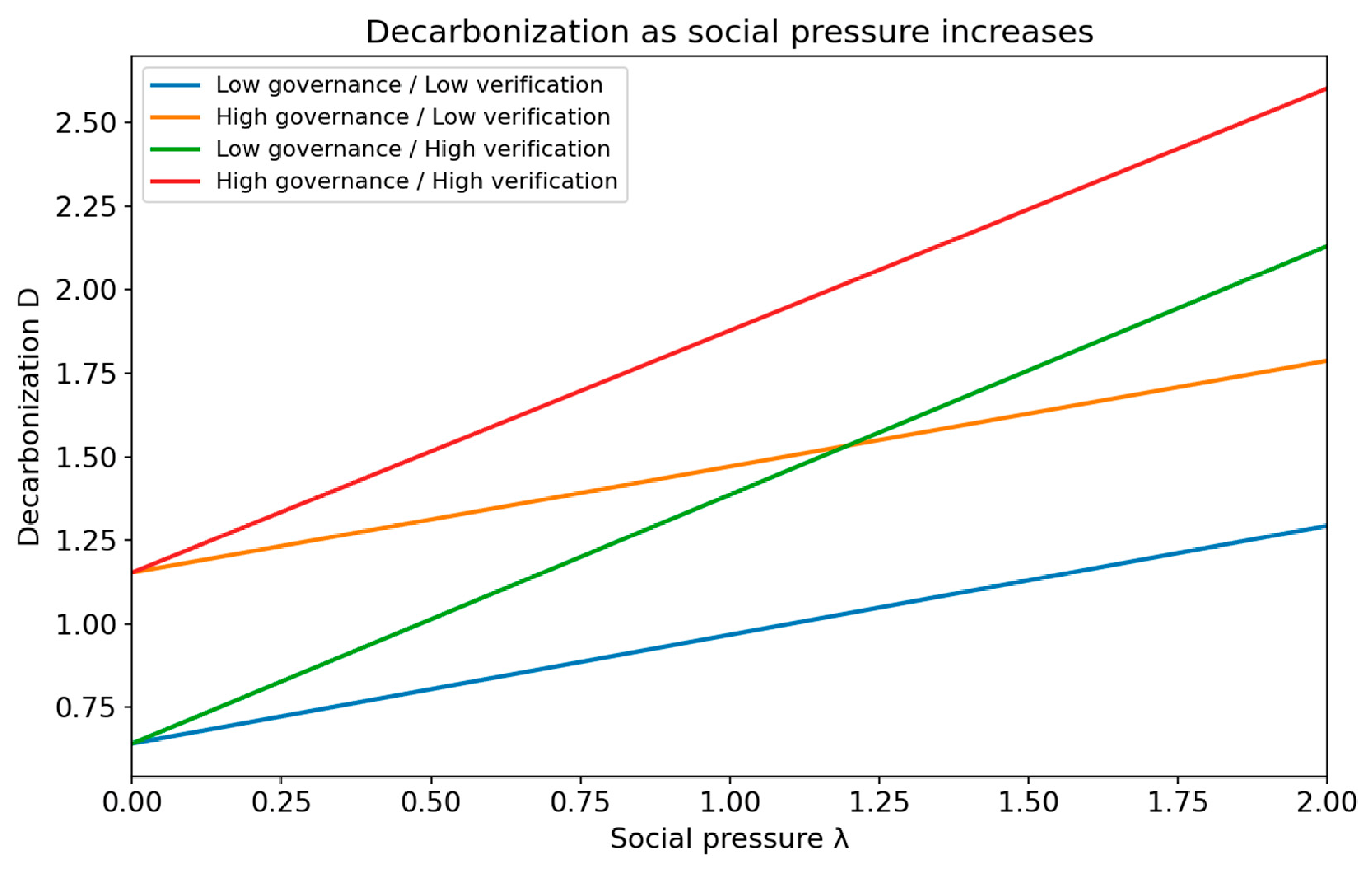
The composition of the response is equally important. Figure C2 shows assessment-oriented effort. Under low verification, r becomes positive at relatively modest levels of pressure and then increases linearly with pressure. High verification sharply compresses this response. High governance further lowers r because assessment-oriented activity is less effective when ρ(γ) is smaller.

Figure 2. Assessment-oriented effort as social pressure increases across governance and verification regimes.

Figure 2. Assessment-oriented effort as social pressure increases across governance and verification regimes.

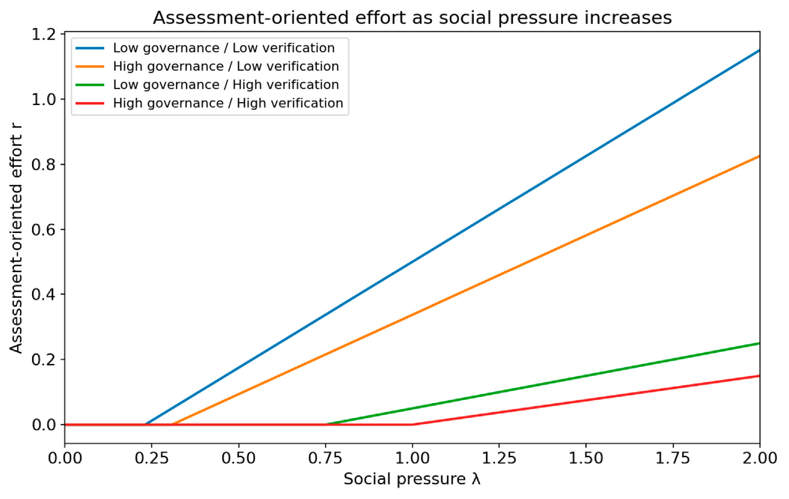
Table 1 reports the outcomes at λ=2 for these four regimes. All entries and differences are computed from unrounded choices and rounded only for display.

C.3. Pressure and Corporate Operating Efficiency

Figure C3 illustrates the non-monotonic efficiency mechanism developed in Section 4.3 at imperfect verification. In this illustration, ω<1 in both governance regimes and the stakeholder-induced response is favorably aligned with underweighted private operating benefits, so Γθ>0 at λ=0 for both θ=0.35 and θ=0.80. Assessment-oriented activity remains at its local corner at λ=0 and enters only after pressure becomes sufficiently strong. Moderate stakeholder pressure therefore raises operating efficiency initially. Once pressure becomes sufficiently strong, however, additional genuine activity and assessment-oriented expenditure push the firm beyond its operating-efficiency-maximizing allocation.

Figure 3. Corporate operating efficiency as social pressure increases across governance and verification regimes.

Figure 3. Corporate operating efficiency as social pressure increases across governance and verification regimes.

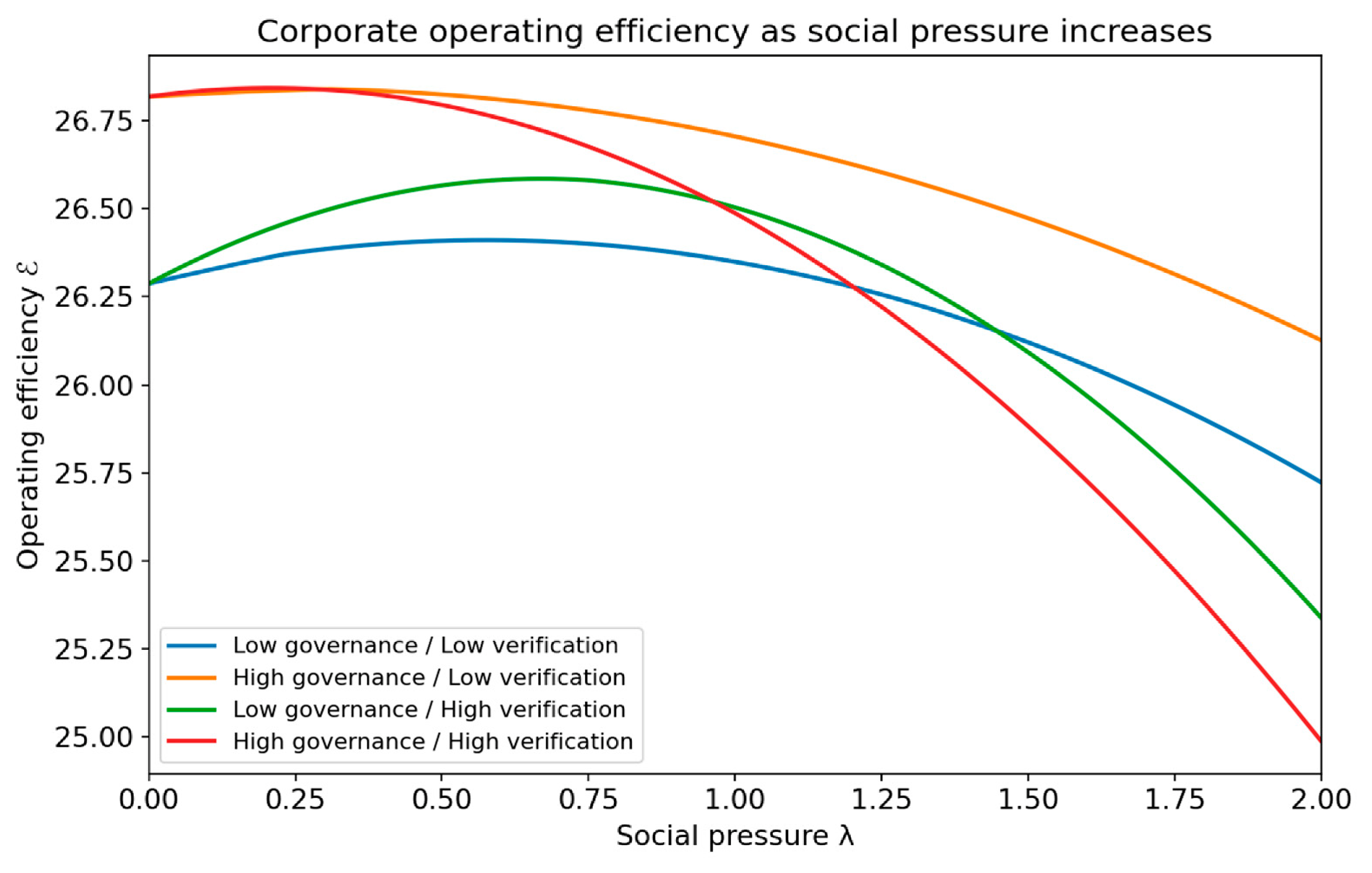
Operating efficiency reaches a positive interior maximum of the illustrated pressure interval in every regime; Table C2 reports the maximizing values. The high-governance/low-verification maximum occurs exactly where assessment-oriented effort enters. Governance changes several channels in this exercise, so the comparison does not isolate managerial internalization.

The illustration should not be read as implying that a particular numerical level of pressure is optimal in practice. The economically relevant point is qualitative: when an internal distortion is present, the operating-efficiency effect of stakeholder pressure can change sign. This is why a linear empirical specification relating sustainability pressure to firm performance may conceal important heterogeneity.

For completeness, operating efficiency along the pressure path is

$ℰ$(λ) = νx*(λ) + A_D[d*(λ)] + A_H[h*(λ)]

(C9)

Equation (C9) defines a continuous, piecewise-quadratic function over λ∈[0,2], with a kink when assessment-oriented activity enters. Evaluating the stationary points of each piece, the entry point, and the interval endpoints gives the maxima in Table C2.

Table 2. Operating-efficiency maxima over the illustrated pressure interval λ∈[0,2].

Regime	λ^E
Low governance / Low verification	0.575
High governance / Low verification	0.308
Low governance / High verification	0.669
High governance / High verification	0.209

Table 2. Operating-efficiency maxima over the illustrated pressure interval λ∈[0,2].

Regime	λ^E
Low governance / Low verification	0.575
High governance / Low verification	0.308
Low governance / High verification	0.669
High governance / High verification	0.209

All four maxima exceed operating efficiency at zero pressure, while efficiency at λ=2 is below its zero-pressure value. This verifies initial correction and subsequent decline within the illustrated interval. Appendix B.3’s result for an unbounded pressure domain requires its additional large-pressure condition. The numerical governance comparison changes internalization, implementation costs, and communication effectiveness together.

C.4. Carbon Weight and Decarbonization

The final exercise varies the metric carbon weight α_m while holding λ = 2 and γ = 0 fixed. Verification again increases genuine activity, but the extent to which the resulting improvement in S appears as decarbonization depends directly on the weight assigned to carbon within the performance metric.

Table 3. Carbon-weight sensitivity at λ=2 and γ=0.

Metric carbon weight α_m	D: low θ	D: high θ	Change in D	Change in S
0.20	0.772	0.940	0.167	0.736
0.40	0.902	1.237	0.335	0.836
0.60	1.033	1.535	0.502	1.004
1.00	1.293	2.130	0.837	1.540
1.40	1.553	2.726	1.172	2.343

Table 3. Carbon-weight sensitivity at λ=2 and γ=0.

Metric carbon weight α_m	D: low θ	D: high θ	Change in D	Change in S
0.20	0.772	0.940	0.167	0.736
0.40	0.902	1.237	0.335	0.836
0.60	1.033	1.535	0.502	1.004
1.00	1.293	2.130	0.837	1.540
1.40	1.553	2.726	1.172	2.343

When α_m = 0.20, increasing verification from 0.35 to 0.80 raises S by 0.736 but decarbonization by only 0.167. With α_m = 1.00, the same verification improvement raises decarbonization by 0.837. At the limiting boundary α_m = 0, outside the maintained positive-carbon-weight assumption, verification can raise S entirely through the non-carbon outcome without changing d in this separable illustration.

Holding λ=2 and γ=0 fixed, the decarbonization formula is

d*(α_m,θ) = [ωa_D + λθα_m − νmc_D]/[νmk_D + ωb_D],

(C10)

so the verification effect on d is proportional to α_m. Table C3 reports differences calculated from unrounded choices for θ=0.35 and θ=0.80; its displayed endpoints need not subtract to the displayed change after rounding.

References

- Azar, J., Duro, M., Kadach, I., & Ormazabal, G. (2021). The Big Three and corporate carbon emissions around the world. Journal of Financial Economics, 142(2), 674–696. [CrossRef]
- Baker, G. P. (1992). Incentive contracts and performance measurement. Journal of Political Economy, 100(3), 598–614. [CrossRef]
- Baker, G. P. (2002). Distortion and risk in optimal incentive contracts. Journal of Human Resources, 37(4), 728–751. [CrossRef]
- Baron, D. P. (2001). Private politics, corporate social responsibility, and integrated strategy. Journal of Economics & Management Strategy, 10(1), 7–45. [CrossRef]
- Bénabou, R., & Tirole, J. (2010). Individual and corporate social responsibility. Economica, 77(305), 1–19. [CrossRef]
- Berg, F., Kölbel, J. F., & Rigobon, R. (2022). Aggregate confusion: The divergence of ESG ratings. Review of Finance, 26(6), 1315–1344. [CrossRef]
- Berrone, P., Fosfuri, A., & Gelabert, L. (2017). Does greenwashing pay off? Understanding the relationship between environmental actions and environmental legitimacy. Journal of Business Ethics, 144(2), 363–379. [CrossRef]
- Bolton, P., & Kacperczyk, M. (2021). Do investors care about carbon risk? Journal of Financial Economics, 142(2), 517–549. [CrossRef]
- Castillo-Merino, D., & Rodríguez-Pérez, G. (2021). The effects of legal origin and corporate governance on financial firms’ sustainability performance. Sustainability, 13(15), 8233. [CrossRef]
- Christensen, H. B., Hail, L., & Leuz, C. (2021). Mandatory CSR and sustainability reporting: Economic analysis and literature review. Review of Accounting Studies, 26(3), 1176–1248. [CrossRef]
- Delmas, M. A., & Burbano, V. C. (2011). The drivers of greenwashing. California Management Review, 54(1), 64–87. [CrossRef]
- Dyck, A., Lins, K. V., Roth, L., & Wagner, H. F. (2019). Do institutional investors drive corporate social responsibility? International evidence. Journal of Financial Economics, 131(3), 693–714. [CrossRef]
- Eccles, R. G., Ioannou, I., & Serafeim, G. (2014). The impact of corporate sustainability on organizational processes and performance. Management Science, 60(11), 2835–2857. [CrossRef]
- Feltham, G. A., & Xie, J. (1994). Performance measure congruity and diversity in multi-task principal/agent relations. The Accounting Review, 69(3), 429–453. https://www.jstor.org/stable/248233. [CrossRef]
- Ferrell, A., Liang, H., & Renneboog, L. (2016). Socially responsible firms. Journal of Financial Economics, 122(3), 585–606. [CrossRef]
- Fischer, P. E., & Verrecchia, R. E. (2000). Reporting bias. The Accounting Review, 75(2), 229–245. [CrossRef]
- Flammer, C. (2021). Corporate green bonds. Journal of Financial Economics, 142(2), 499–516. [CrossRef]
- Gillan, S. L., Koch, A., & Starks, L. T. (2021). Firms and social responsibility: A review of ESG and CSR research in corporate finance. Journal of Corporate Finance, 66, 101889. [CrossRef]
- Global Reporting Initiative. (2018). GRI 303: Water and effluents 2018. https://www.globalreporting.org/publications/documents/english/gri-303-water-and-effluents-2018/.
- Hart, O., & Zingales, L. (2017). Companies should maximize shareholder welfare not market value. Journal of Law, Finance, and Accounting, 2(2), 247–274. [CrossRef]
- Hart, S. L., & Ahuja, G. (1996). Does it pay to be green? An empirical examination of the relationship between emission reduction and firm performance. Business Strategy and the Environment, 5(1), 30–37. [CrossRef]
- Heinkel, R., Kraus, A., & Zechner, J. (2001). The effect of green investment on corporate behavior. Journal of Financial and Quantitative Analysis, 36(4), 431–449. [CrossRef]
- Holmström, B. (1999). Managerial incentive problems: A dynamic perspective. Review of Economic Studies, 66(1), 169–182. [CrossRef]
- Holmström, B., & Milgrom, P. (1991). Multitask principal-agent analyses: Incentive contracts, asset ownership, and job design. Journal of Law, Economics, and Organization, 7(Special Issue), 24–52. [CrossRef]
- Liu, Y., Dijst, M., Geertman, S., & Cui, C. (2017). Social sustainability in an ageing Chinese society: Towards an integrative conceptual framework. Sustainability, 9(4), 658. [CrossRef]
- Lyon, T. P., & Maxwell, J. W. (2011). Greenwash: Corporate environmental disclosure under threat of audit. Journal of Economics & Management Strategy, 20(1), 3–41. [CrossRef]
- Lyon, T. P., & Montgomery, A. W. (2015). The means and end of greenwash. Organization & Environment, 28(2), 223–249. [CrossRef]
- Marquis, C., Toffel, M. W., & Zhou, Y. (2016). Scrutiny, norms, and selective disclosure: A global study of greenwashing. Organization Science, 27(2), 483–504. [CrossRef]
- Oehmke, M., & Opp, M. M. (2025). A theory of socially responsible investment. Review of Economic Studies, 92(2), 1193–1225. [CrossRef]
- Pástor, Ľ., Stambaugh, R. F., & Taylor, L. A. (2021). Sustainable investing in equilibrium. Journal of Financial Economics, 142(2), 550–571. [CrossRef]
- Pineiro-Chousa, J., Vizcaíno-González, M., & López-Cabarcos, M. Á. (2016). Reputation, game theory and entrepreneurial sustainability. Sustainability, 8(11), 1196. [CrossRef]
- Porter, M. E., & van der Linde, C. (1995). Toward a new conception of the environment-competitiveness relationship. Journal of Economic Perspectives, 9(4), 97–118. [CrossRef]
- Simnett, R., Vanstraelen, A., & Chua, W. F. (2009). Assurance on sustainability reports: An international comparison. The Accounting Review, 84(3), 937–967. [CrossRef]
- Stein, J. C. (1989). Efficient capital markets, inefficient firms: A model of myopic corporate behavior. Quarterly Journal of Economics, 104(4), 655–669. [CrossRef]
- Wang, L., Li, W., & Qi, L. (2020). Stakeholder pressures and corporate environmental strategies: A meta-analysis. Sustainability, 12(3), 1172. [CrossRef]
- World Resources Institute, & World Business Council for Sustainable Development. (2004). The greenhouse gas protocol: A corporate accounting and reporting standard (revised edition). https://ghgprotocol.org/sites/default/files/standards/ghg-protocol-revised.pdf.
Disclaimer/Publisher’s Note: The statements, opinions and data contained in all publications are solely those of the individual author(s) and contributor(s) and not of MDPI and/or the editor(s). MDPI and/or the editor(s) disclaim responsibility for any injury to people or property resulting from any ideas, methods, instructions or products referred to in the content. |
© 2026 by the authors. Licensee MDPI, Basel, Switzerland. This article is an open access article distributed under the terms and conditions of the Creative Commons Attribution (CC BY) license (http://creativecommons.org/licenses/by/4.0/).
Copyright: This open access article is published under a Creative Commons CC BY 4.0 license, which permit the free download, distribution, and reuse, provided that the author and preprint are cited in any reuse.