
Submitted:
08 October 2026
Posted:
09 October 2026
You are already at the latest version
Abstract
Pilot samples arise naturally in two-stage statistical procedures, where preliminary observations are used to estimate an unknown optimal allocation before the remaining observations are assigned. The central question is the choice of pilot size. A small pilot gives poor estimation of the optimal allocation, while a large pilot commits too many observations before that allocation is known. Under allocation MSE and regular parametric estimation, these two effects lead to a sharp balance. The pilot size grows as the two-thirds power of the total sample size. The square-root pilot is first-order adequate, whereas the two-thirds rule gives the higher-order balance between estimation and early commitment. Four pilot-size regimes are considered to show the effect of choosing the pilot below, at, or above this order. The result is general and does not depend on a particular distribution. Exponential lifetime populations are used as an application for which the optimal allocation can be obtained explicitly. Reliability and medical examples illustrate implementation of the rule.
Keywords:
two-stage allocation
; regular parametric model
; pilot estimation
; worst-case MSE
; pilot sample
; asymptotic optimality
; exponential lifetime model
; reliability
; hazard rate
; failure rate
MSC: 62K05; 62L05; 62N05
1. Introduction
Pilot samples arise whenever preliminary observations are used to learn unknown features of a statistical problem before the main sampling decision is made. This basic structure appears in estimation, allocation, reliability, engineering experiments, medical studies, clinical trials, and adaptive design. The terminology differs across fields, but the underlying question is the same: how much information should be collected before the principal decision is made?
The statistical origin of this idea can be traced at least to Stein [1]. Stein (1945) introduced a two-stage procedure in which information obtained from an initial sample is used to determine subsequent sampling when an unknown variance prevents direct implementation of the desired procedure. The importance of the construction extends beyond that particular problem. It established a basic principle of two-stage methodology: learn an unknown quantity in Stage 1 and use that information to determine Stage 2.
The size of the first stage soon became a problem in its own right. Seelbinder [23] studied Stein’s sampling scheme and developed a method for determining the size of the first part of the sample. Moshman [24] returned explicitly to the initial-sample-size problem and proposed a practical rule for selecting that first sample. These early papers show that pilot-size selection has been part of two-stage methodology almost from its beginning. The first-stage sample is not merely preliminary; its size affects the performance of the complete procedure.
A parallel development occurred in sequential estimation. Anscombe [25] developed large-sample theory for estimation with data-dependent sample sizes. Chow and Robbins [26] established an influential sequential procedure for fixed-width confidence intervals. Woodroofe [3,4] subsequently developed higher-order sequential theory and nonlinear renewal methods. Together, these developments provided much of the theoretical foundation for comparing fixed-sample, two-stage, multistage, and sequential procedures.
Two-stage procedures occupy an important position between fixed and sequential sampling. A fixed procedure makes all sampling decisions before observing the data. A sequential procedure may repeatedly use accumulated information to modify sampling. A two-stage procedure permits one principal adaptation: Stage 1 provides information and Stage 2 uses that information. This structure retains much of the simplicity of a fixed experiment while allowing the design to respond to information that was unavailable initially. Colton and McPherson [37] made this middle position explicit by comparing two-stage plans with fixed-sample-size procedures and Wald sequential probability-ratio plans. Their comparison illustrates a recurring theme of the subject: a small number of well-placed adaptations can recover a substantial part of the efficiency of full sequential sampling without requiring observation-by-observation decisions. The same principle became important in allocation problems. When the optimal allocation depends on unknown parameters, the optimal allocation cannot be implemented directly; the unknown quantities must first be estimated. Rekab [5] studied asymptotic efficiency in sequential designs for estimation in 1989. Rekab [6] then developed a nearly optimal two-stage procedure in 1992 using a square-root-order first stage, providing an important benchmark for the present pilot-size problem. Subsequent work extended this research line to reliability [7], two-stage allocation [8], higher-order sequential MSE [9], and multistage software-reliability allocation [10]. Mukhopadhyay [11] developed related sequential estimation methodology. This progression—sequential efficiency, two-stage approximation, reliability allocation, and multistage refinement—provides the immediate historical background for the present rate-balance approach.
Few-stage design provided another important direction. Hardwick and Stout [14] studied optimal two- and three-stage designs and showed that the location of the adaptation points can have an important effect on performance. For consistency with the present paper, we use M for the total sample size and L for the first-stage size when discussing their work, regardless of the notation used in the original paper. Benkamra, Terbeche, and Tlemcani [15] developed one-, two-, and three-stage procedures for estimating a product of Bernoulli proportions. These results reinforce a central point: broad asymptotic conditions may guarantee validity without determining the most effective first-stage size.
Clinical trials developed two especially important two-stage traditions. In early anticancer drug development, Gehan [33] used double-sampling ideas to decide whether a new treatment should continue beyond an initial group of patients, and Simon [34] later derived optimal and minimax two-stage Phase II designs that control type-I and type-II error while reducing expected sample size when activity is low. These designs made two-stage decision rules part of routine clinical-trial methodology and showed that the first-stage size can directly determine both ethical exposure and statistical efficiency.
A second clinical tradition uses Stage 1 to learn nuisance or design quantities and then modifies the remainder of the trial. Wittes and Brittain [35] introduced the internal-pilot concept for recalculating sample size from interim estimates while retaining the pilot observations in the final analysis. Bauer and Köhne [36] developed a general adaptive-interim testing framework. Proschan [27] reviewed two-stage sample-size re-estimation based on nuisance parameters, and Friede and Kieser [28] reviewed internal-pilot sample-size recalculation. Birkett and Day [38] studied internal pilots for estimating sample size, while Proschan and Hunsberger [39] developed a designed two-stage extension based on conditional power. Group-sequential methodology and modern adaptive-design practice are treated systematically by Jennison and Turnbull [40] and Bhatt and Mehta [41]. Although these clinical objectives differ from the allocation MSE criterion, they embody the same learn-then-act architecture: early data are collected to improve a later design decision, and the amount of early information must be chosen carefully.
The same pilot-size question arises in many applied settings in which preliminary observations are used to estimate unknown quantities before later observations or resources are assigned. Examples include comparative and accelerated life testing, degradation studies, reliability demonstration, component and system testing, software reliability, clinical and medical studies, engineering experiments, manufacturing and quality control, adaptive sampling, agricultural experiments, survey sampling, online experimentation, and data-acquisition problems in machine learning. In reliability and lifetime modeling, standard references include Meeker and Escobar [16] and Lawless [17], with more recent design examples in [18,19]. A related modern two-wave result is given by Yamin [20], while a later sequential reliability application is given by Zarzour and Rekab [22].
Despite this long development, the first-stage-size problem appears in different forms across the literature. Stein-type procedures use the first stage to determine subsequent sample size. Sequential estimation determines when sufficient information has accumulated. Phase II clinical designs use Stage 1 to decide whether recruitment should continue. Internal-pilot procedures revise total sample size or nuisance-parameter estimates. Adaptive-interim methods modify prespecified aspects of a trial while preserving valid inference. Adaptive allocation procedures estimate where later observations should be assigned. Few-stage procedures determine when a limited number of adaptations should occur. These problems share a common learn-then-act structure, but their objectives and error criteria differ. Consequently, no single pilot-size rule should be expected to be optimal for every two-stage problem.
The present article considers an important general class of these problems. A pilot sample is used to estimate an unknown preferred allocation, and the remaining observations are then assigned using that estimate. The central question is the choice of pilot size. A pilot that is too small produces inaccurate estimation of the preferred allocation. A pilot that is too large improves estimation but commits too many observations before the preferred allocation is known. Pilot-size optimality therefore requires a balance between learning and early commitment.
Let M denote the total sample size and L the Stage-1 pilot size. Classical two-stage theory commonly requires the pilot to increase while remaining a vanishing fraction of the total sample. These conditions establish first-order validity, but they permit many possible pilot sizes and do not determine how rapidly the pilot should grow.
The principal contribution of this article is to make that balance explicit. Under allocation MSE and regular parametric estimation, the error produced by estimating the unknown allocation is of order , whereas the error created by observations committed during Stage 1 is of order . Balancing these two effects gives the two-thirds pilot rule: the pilot grows as the two-thirds power of the total sample size.
This result also clarifies the role of the square-root pilot. A square-root pilot is first-order adequate, but it remains on the estimation-dominated side of the problem. Increasing the pilot beyond square-root order improves the balance until the two-thirds order is reached. At the two-thirds order, estimation error and early-commitment error have the same asymptotic order. Beyond this point, additional pilot observations reduce flexibility faster than they improve the relevant worst-case allocation error. These observations lead naturally to four pilot-size regimes.
The theory developed here is general. It is not tied to a particular distribution, lifetime model, reliability problem, or scientific application. Its essential ingredients are a pilot estimate of an unknown preferred allocation, a second-stage decision based on that estimate, and an MSE criterion measuring departure from the optimal allocation. To illustrate the general theory, two exponential lifetime populations are considered in detail. The exponential model is useful because the optimal allocation can be obtained explicitly and the consequences of pilot-size selection can be seen directly. Reliability and medical examples illustrate implementation; they do not define the scope of the theory.
Viewed historically, the present article returns to a question already visible in the work following Stein: how large should the initial sample be? The answer developed here is a rate balance between learning the unknown allocation and preserving enough observations for Stage 2 to act on what has been learned.
The remainder of the article is organized as follows. Section 2 formulates the general two-stage allocation problem and the uniform MSE criterion. Section 3 establishes the pilot-size result and develops the four pilot-size regimes. Section 4 applies the theory to exponential lifetime populations. The following sections present practical, reliability, medical, and numerical illustrations, while technical details are collected in the Appendices.
2. General Two-Stage Formulation
This section isolates the mechanism that drives the paper. The probability model is left general: there is an optimal allocation that would be used if the unknown parameters were known, a pilot that estimates that allocation, and a second stage that can use only observations not already committed.
Pilot-size optimality therefore has two components: statistical learning, which determines how accurately the pilot estimates the preferred allocation, and operational flexibility, which determines how much of the final design can still be changed after Stage 1.
Throughout this paper, M is the total sample size; L is the total first-stage size; and are the first-stage allocations; and are the final allocations; q is the first-stage fraction assigned to population 1; is the optimal allocation fraction when is known; is its first-stage estimate; and
is the final fraction assigned to population 1.
- Rate convention.
In the main text, asymptotic comparisons are stated directly in words whenever possible. The symbol is used only in displayed matching-rate summaries. Detailed compact asymptotic notation is confined to the Appendix. Finally, refers to the scale or order of the pilot, not necessarily the exact finite-M integer choice.
M is the total size of the experiment, whereas L is the number of observations spent learning before the main allocation decision. Thus provides increasing information in Stage 1, while ensures that this learning stage remains a vanishing fraction of the complete experiment.
For , let observations from population i follow a regular parametric model indexed by an unknown parameter . We write this generically as
This notation deliberately leaves the probability model unspecified. Theorem 1 requires only that the ideal allocation fraction vary smoothly with the unknown parameter and that the Stage-1 data estimate this fraction with MSE of order . Thus the main theorem applies beyond any single named distributional family.
Let
If were known, suppose the preferred fixed-design allocation assigns the fraction
of the total sample to population 1. Thus means that, if were known before sampling, about of the total observations would ideally be assigned to population 1 and to population 2. The function can come from minimizing variance, maximizing information, or another smooth fixed-design objective.
Let M be the total number of observations available. Let L be the total Stage-1, or pilot, sample size. Of these L pilot observations, are assigned to population 1 and to population 2, so
We write approximately equal to and approximately equal to , where q is the Stage-1 fraction assigned to population 1. After both stages are complete, let and be the final totals, with
From the pilot data we estimate the unknown parameter and then estimate the ideal allocation fraction by the plug-in value .
For convenience, we first truncate the pilot estimate to : replace by . Because , this truncation cannot increase squared allocation error. We continue to write for the truncated estimator below.
Truncation to is only a safeguard against an estimated fraction falling outside the range of possible allocation fractions. It does not change a valid estimate already between 0 and 1, and it cannot increase squared error because the true allocation fraction itself lies in .
Thus,
Because Stage-1 observations cannot be reassigned, they impose hard feasibility limits on Stage 2. Once observations have been assigned to population 1 and to population 2, the final totals must satisfy
Equivalently, the final fraction must remain between and . Stage 2 can add observations, but it cannot undo a Stage-1 assignment:
The feasible two-stage allocation rule is
The feasible interval is the range of final allocation fractions that remain possible after Stage 1. Since the observations already assigned to population 1 and the observations already assigned to population 2 cannot be reassigned, the final fraction assigned to population 1 cannot be smaller than or larger than . If lies inside this interval, it is used directly. If it lies below or above the interval, the corresponding feasible boundary is used instead. Thus Stage 2 moves the final allocation as close as possible to the estimated preferred allocation without changing observations already assigned in Stage 1. The term is only the integer-rounding adjustment, and its absolute value is at most .
3. General Pilot-Size Principle and the Four Cases
The first-stage-size question has appeared repeatedly since the early development of two-stage sampling. Stein showed why an initial sample can be useful; Seelbinder and Moshman showed that the size of that initial sample is itself a design problem; Woodroofe developed higher-order sequential tools; and Rekab [5,6] connected asymptotic efficiency with nearly optimal two-stage procedures. The present section places these ideas on a single pilot-growth scale.
The square-root first stage in Rekab [6] is especially important historically. It supplies a familiar first-order benchmark. The new question is what happens when we compare different pilot growth rates under a criterion that charges both for imperfect learning and for observations committed too early. The answer is not a single isolated exponent but a complete four-regime picture.
M denotes the total sample size and L denotes the total Stage-1 pilot size. The exponent is used when the pilot is written as L proportional to . The optimal allocation is the allocation that would be selected if the unknown model parameters were known. In the two-stage procedure those parameters are estimated from the pilot, and the remaining observations are assigned using the resulting estimated optimal allocation.
Theorem 1
(Sharp worst-case MSE order and minimax-rate optimality). Under the regularity framework above, for every fixed pilot split q bounded away from 0 and 1 and any pilot sequence with
there exist positive constants and such that, for all sufficiently large M,
Moreover, no regular two-stage rule in the stated class can improve this worst-case order uniformly; hence the feasible plug-in rule is minimax-rate optimal.
Theorem 1 has a simple interpretation: is the learning error from estimating the preferred allocation with only L pilot observations, while is the early-commitment error created by assigning a fraction of the experiment before that allocation is known. Increasing L decreases the first effect but increases the second.
The matching upper and lower bounds establish sharpness: the feasible rule attains the stated order, while suitable interior and near-boundary parameter configurations show that neither component can be removed uniformly.
Here “sharp” means that both orders are intrinsic to the problem: the upper bound shows that the proposed rule attains their sum, while the lower bound shows that regular two-stage rules cannot uniformly improve both orders over the stated parameter class.
The regularity conditions ensure stable pilot estimation, smooth variation of the optimal allocation with the unknown parameters, and parameter configurations that expose the Stage-1 allocation effect. Each condition supports a distinct part of the MSE decomposition. If the estimation rate or allocation structure changes, the balancing exponent can change.
The theorem identifies two unavoidable errors. Pilot estimation contributes order , whereas irreversible Stage-1 assignments contribute order in the worst case. Their sum therefore determines the sharp uniform MSE order.
Corollary 1
(Unique minimax rate-optimal exponent). Let
In the setting of Theorem 1, both the feasible plug-in rule and the worst-case MSE over the stated regular two-stage class have order
The worst-case convergence exponent is therefore
It is uniquely maximized by
and the resulting worst-case MSE has rate
The power-law form is a device for comparing growth rates, not a rigid finite-sample prescription. The exponent simply measures how rapidly the pilot grows relative to M.
Writing turns pilot growth into a one-parameter comparison. The rate is controlled by the slower of the learning term and the early-commitment term .
The balance is immediate on the exponent scale: with L proportional to , learning contributes and early commitment contributes . Their slower decay is best when the exponents are equal, giving . Technical details are collected in Appendix A.
To see the crossing directly, set the two decay exponents equal:
This gives
At that value neither learning error nor early commitment dominates the other; both decrease at the same rate .
For a planned total size M, is therefore a practical center for Stage 1, not an exact integer command. Nearby feasible choices can be compared when finite-sample calculations are available.
3.1. Four Pilot-Size Cases
The four cases locate the pilot relative to the balance point: Cases 1 and 2 are learning-dominated, Case 3 gives the exact asymptotic balance, and Case 4 is commitment-dominated. This makes clear why either under-piloting or over-piloting worsens the leading error.
The representation
makes the pilot size easy to compare across different total sample sizes. A larger means a larger Stage-1 pilot. The pilot has a gain because more data improve estimation of the unknown optimal allocation, but it also has a cost because more observations are committed before that allocation is known. The four cases below show how these two forces change as increases.
Case 1: — small to square-root pilot.
In this region, estimation is the dominant limitation. When , the pilot grows even more slowly than square-root order and the allocation is learned too slowly for the higher-order criterion. At , the pilot reaches the familiar square-root scale. This may be sufficient for first-order behavior, but the higher-order MSE is still dominated by estimation. In practical terms, the design preserves excellent Stage-2 flexibility, but it has not yet used enough Stage-1 information to obtain the best worst-case rate.
Example for Case 1.
If , a square-root pilot has size about 32. Roughly 968 observations remain for Stage 2, so flexibility is high. The weakness is that the estimated optimal allocation is based on only about 32 pilot observations. The procedure can be first-order adequate while still carrying a comparatively large pilot-estimation error.
Published clinical example for Case 1 ().
Cheung and Kaufmann [42] examined an internal-pilot strategy for early-phase stroke trials in which the first stage contained 30 patients per treatment arm. When the true placebo response rate was lower than originally assumed, the adaptive two-stage design maintained adequate power while using a smaller average final sample than a conservative fixed design; when the placebo rate was higher, it retained approximately the target power. Their calculations also showed that reducing the internal pilot to 15 patients per arm could produce substantially greater sample-size inflation. Their study did not use the present allocation rule. Rather, it provides a concrete finite-sample illustration of the mechanism emphasized here for : a pilot that is too small can estimate the quantity driving the second-stage decision too noisily, even though substantial Stage-2 flexibility remains.
Case 2: — the useful intermediate region.
The pilot is larger than square-root order, so the optimal allocation is estimated more accurately, while most of the total sample still remains available for Stage 2. As increases in this interval, the pilot-estimation term improves faster than the Stage-1 allocation effect term becomes harmful. Thus moving from to , for example, produces a genuine higher-order gain under the present criterion.
Example for Case 2.
With , gives a pilot of about 45 and gives a pilot of about 63. The larger pilot uses only about 18 additional observations but provides more information for estimating the allocation. The gain is worthwhile because the experiment still retains more than 900 observations for Stage 2.
Published application for Case 2.
Nelson and Kielpinski [30] developed optimum censored accelerated-life-test plans and illustrated them with a temperature-accelerated electrical-insulation experiment under an Arrhenius model. Their study shows why pilot information about lifetime behavior and stress response can matter before the remaining units are allocated. An intermediate pilot, , has a natural role when more stable preliminary estimation is desired than under square-root sampling, but the experiment still benefits from retaining substantial Stage-2 flexibility.
Case 3: — the balance point.
Here the pilot-estimation contribution and the Stage-1 allocation effect contribution have the same asymptotic order. Neither dominates. This is the unique crossing point of the two error rates under pilot estimation and the allocation MSE criterion. The value is therefore not an arbitrary numerical recommendation; it is obtained by balancing the statistical gain from estimation against the reduction in Stage-2 flexibility.
Example for Case 3.
If ,
The pilot uses about 100 observations and leaves about 900 for Stage 2. Compared with a square-root pilot of about 32, the design deliberately spends more observations on estimation, but it still preserves most of the experiment for the adaptive second stage.
Published application for Case 3.
Hong et al. [31] re-executed the ANZ 9311 metastatic-breast-cancer trial using adaptive designs. The original trial recruited 235 participants, and the retrospective analysis showed that adaptive designs could materially change power or average sample size. The study did not use the present rule; it illustrates a setting in which allocation and sample-size inefficiency have real consequences because recruitment is limited and each observation is consequential. Such settings motivate the stronger second-order protection associated here with .
Case 4: — oversized pilot.
Beyond the balance point, the Stage-1 estimates continue to become more accurate, but the gain is no longer large enough to compensate for the observations already committed. The Stage-1 allocation effect term becomes dominant, and the worst-case convergence rate deteriorates as approaches 1. The procedure is now Stage-1 allocation effect-limited rather than estimation-limited.
Example for Case 4.
With and , the pilot contains about 251 observations. The pilot estimates are more accurate than with , but roughly one quarter of the entire experiment has already been assigned before the optimal allocation is known. If the true optimal allocation is strongly unbalanced, Stage 2 may no longer have enough freedom to correct the early assignments.
Published application for Case 4.
Shohji, Mori, and Orii [32] performed thermal-cycle tests on chip-scale-package solder joints under several cycling conditions and modeled thermal-fatigue life. Reliability programs of this type can require long, tightly controlled laboratory testing and expensive specimens. An investigator may therefore choose a larger preliminary stage to obtain highly stable engineering estimates before a costly second phase. In the present theory, however, is an operational choice rather than an efficiency improvement: additional pilot stability is purchased by committing too much of the total experiment before adaptation.
The four cases tell one continuous story. A very small pilot preserves flexibility but learns too little. Increasing the pilot beyond square-root order improves estimation. At , pilot estimation and Stage-1 allocation are balanced. Increasing the pilot further continues to improve estimation but sacrifices too much flexibility. This is why first-order analysis alone does not determine an efficient pilot size and why the higher-order comparison is practically useful.
The cited studies identify real experimental settings in which the practical value of first-order accuracy, additional pilot stability, second-order protection, or unusually stable preliminary estimation can differ. They are not claimed to have used the present pilot exponent or MSE criterion.
The intermediate region matters because the improvement from one-half to two-thirds is gradual: as increases through this interval, learning improves faster than early commitment becomes costly.
3.2. Choosing the Accuracy Level in Practice
First-order and higher-order efficiency answer different planning questions. Square-root pilots can be adequate when only leading behavior matters and Stage-2 flexibility is paramount. The two-thirds scale is appropriate when the residual allocation MSE itself matters for precision, cost, duration, or scarce experimental units. Exponents above two-thirds should be interpreted as operational choices that deliberately favor unusually stable preliminary estimation over the rate-optimal allocation balance.
3.3. Practical Consequences of Under- and Over-Piloting
Under- and over-piloting fail for different reasons. A pilot that is too small leaves substantial Stage-2 flexibility but estimates the target too noisily; a pilot that is too large estimates the target accurately but leaves too little flexibility to reach it. The four regimes therefore provide a design language for stating explicitly what is gained and what is sacrificed as Stage 1 grows.
Remark 1
(General rate balance). The exponent is one instance of a broader principle. Suppose the dominant worst-case MSE is the sum of a pilot-estimation term of order and a Stage-1 allocation effect term of order . If L has order , the corresponding exponents are and . Balancing them gives
For pilot estimation under the allocation MSE criterion, and , hence . If the estimation rate or error order changes, the balancing exponent changes. The general contribution is therefore the pilot-size balance, not a claim that is universal across all two-stage problems.
More explicitly,
If
then
The best worst-case rate is obtained by balancing the two exponents,
which gives
For the MSE criterion studied here, pilot estimation gives and squared Stage-1 allocation effect gives . Therefore
This also makes the limitation precise: if either the estimation order or the Stage-1 allocation-effect error order changes, the optimal pilot exponent generally changes as well.
Figure 1.
Worst-case convergence exponent versus pilot exponent.
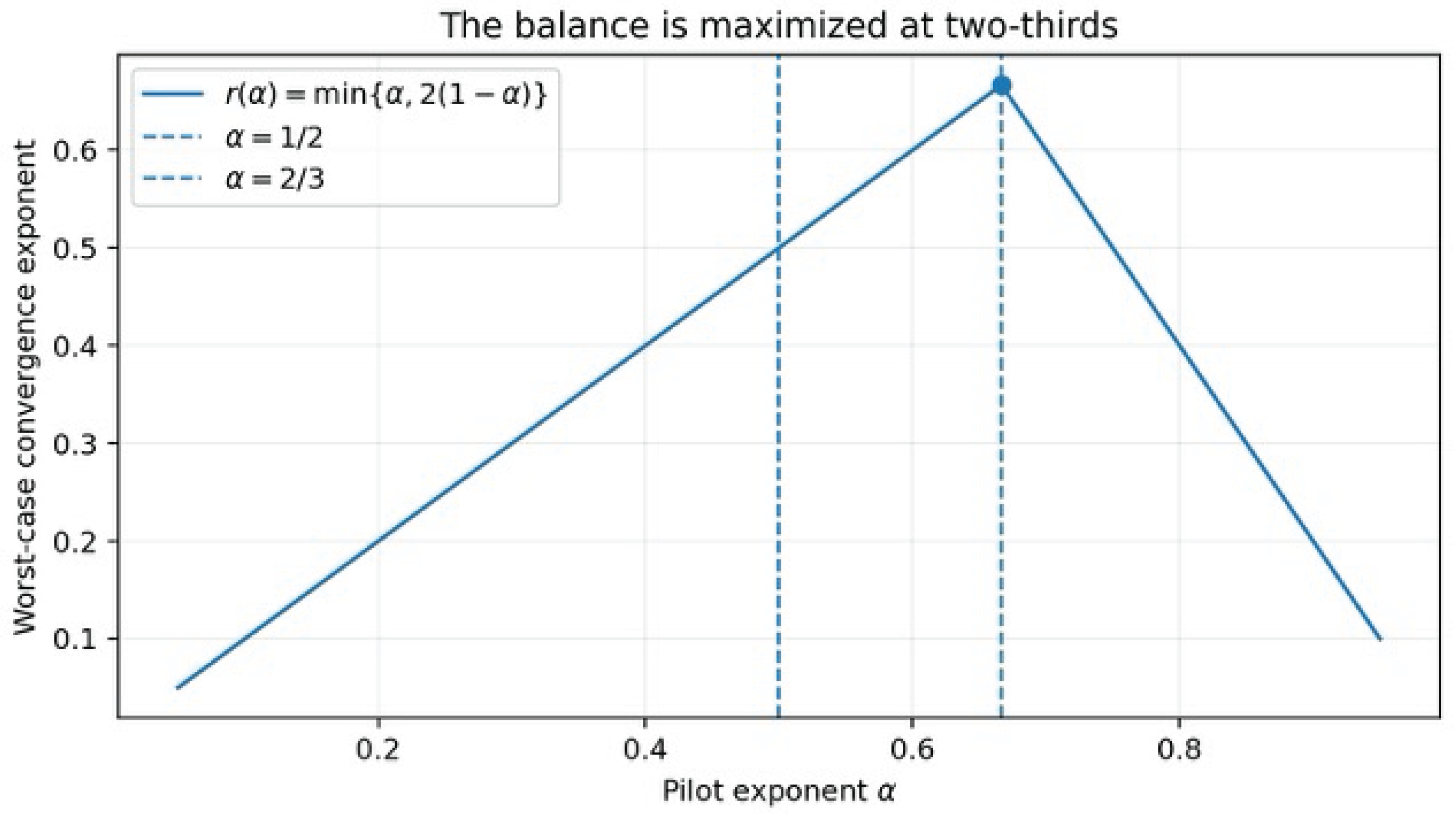
The exponent is optimal for the uniform two-stage criterion considered here and is not claimed to be uniquely optimal under a purely pointwise interior criterion.
4. Application to Exponential Lifetime and Reliability Models
Exponential lifetime models provide a transparent reliability specialization of the general theory. Their constant-hazard structure permits exact calculation, while standard treatments by Meeker and Escobar [16] and Lawless [17] provide the broader lifetime-data context.
The model is used for exposition rather than as an assumption behind Theorem 1. Its value is algebraic: the unbiased hazard-rate estimator has exact inverse-gamma moments, the fixed-sample variance is explicit, and the preferred allocation can be written in closed form.
Think of two products, devices, treatments, or systems whose failure behavior is being compared. The first-stage observations provide an early estimate of the two failure rates. The remaining observations are then allocated using those estimates. The purpose is not to make the two final sample sizes equal; it is to use the fixed total sample more efficiently.
For populations , assume
We consider estimation of the rate difference
A positive means population 1 fails at a higher constant rate than population 2; a negative means the reverse. The goal is not merely to estimate each rate separately, but to divide the fixed total sample M so that the difference is estimated as precisely as possible.
For a fixed sample size in population i, let
be the total observed lifetime. Under exponential sampling, has a gamma distribution. The estimator in (15) rescales so that its expectation is exactly . The requirement is needed because the variance involves the second inverse moment of :
The estimator is unbiased for when and has variance
when .
Theorem 2
(Exact fixed-sample variance and optimal allocation). For with , the unbiased estimator
has variance
The unique continuous minimizer is
and the minimum variance is
Theorem 2 answers a different question from Theorem 1. Theorem 1 tells us how large the pilot should be before learning the unknown allocation. Theorem 2 assumes the exponential rates are known and identifies the allocation we would ideally use. In the actual two-stage procedure, Stage 1 estimates the rates and Stage 2 tries to move the design toward this fixed-sample target. Equations (16)–(19) make the design target explicit. The optimal allocation follows from the exact finite-sample variance, and the population with the larger rate receives more observations because the variance of its unbiased rate estimator scales with . The rule is therefore variance-driven, not importance-driven.
The denominator shows why each population must receive more than two observations for the stated variance formula. Increasing reduces the contribution
Because a larger creates a larger variance contribution, the variance-minimizing design assigns more observations to the population with the larger failure rate.
The finite-sample allocation follows from the exact first two inverse moments of the gamma total lifetime and a one-variable variance minimization. Those algebraic details are given in Appendix B; the main point here is the resulting allocation rule and its reliability interpretation.
Let
Equation (20) rewrites the exact optimal allocation in a more intuitive form. The quantity
is the large-sample optimal fraction for population 1, while the constants 2 and are finite-sample corrections produced by the unbiased exponential-rate estimators. Because these corrections remain bounded as M grows, the exact fraction
approaches P as M grows.
4.1. Reliability Interpretation
In the reliability application, is the complete lifetime of test unit j from population i, with survival , constant hazard , and mean lifetime . The estimand
compares the two failure rates, and the allocation problem asks how to divide a fixed total number of complete lifetimes so that this difference is estimated efficiently.
For population i,
The reliability interpretation is an application of the general theorem, not an assumption behind it. The result follows from the pilot-estimation rate, the Stage-1 allocation effect, the allocation MSE criterion, and boundary richness. The exponential lifetime model is used because it provides an important reliability example in which all relevant quantities can be calculated explicitly.
A simple proportional example makes the allocation rule intuitive. If the first failure rate is approximately twice the second, then the large-sample preferred fraction for population 1 is approximately two-thirds. If the rates are equal, the preferred fraction is one-half. Thus the final design responds to relative statistical variability rather than imposing equal sample sizes by default.
The exponential specialization gives a laboratory or engineering practitioner a complete worked design in which the preferred allocation, the pilot estimators, the internal pilot split, and the final two-stage rule can all be calculated. Its limitation is equally clear: when lifetime hazards are not approximately constant, another reliability model may be more appropriate. The general pilot-size framework remains useful, but the model-specific allocation formula must then be re-derived.
5. Optimal First-Stage Split for the Exponential Model
The total pilot size and the pilot split solve different problems. The general theory determines the scale of the total pilot, while the model-specific calculation below determines how that pilot should be divided between the two exponential populations.
Let the Stage-1 sample sizes be
From the Stage-1 data, define
The pilot estimator of the preferred allocation fraction is
Theorem 3
(Asymptotic distribution of the pilot allocation estimator). Let
If and
then
where
Theorem 3 quantifies the learning part of the two-stage procedure. The pilot fraction is estimated at the usual root-L rate, and the constant multiplying depends on how the pilot is split between the two populations. This makes it possible to optimize the internal pilot allocation separately from the total pilot size.
The expression in (24) separates naturally into a parameter-dependent factor,
and a design-dependent factor,
Only the second factor depends on the pilot split. Thus the question of how to divide the pilot is reduced to a simple deterministic minimization.
Theorem 4
(Balanced pilot split). The asymptotic variance in (24) is uniquely minimized at
At this value,
The balanced split has a simple interpretation. Before the rates are known, neither population should be starved of pilot information. An equal Stage-1 split gives the most stable first-order estimate of the preferred allocation fraction. This does not imply that the final allocation should be equal. The final allocation is generally unequal and depends on the estimated failure rates.
Theorem 4 concerns only the internal composition of Stage 1. It does not determine the total pilot size. The total size is governed by the general rate balance of Theorem 1 and Corollary 1. Thus the two design decisions are complementary:
controls how much data should be spent learning, while
controls how those pilot observations should be divided between the two populations.
The derivation of (23)–(26) follows from the asymptotic distribution of the unbiased exponential-rate estimators and the delta method. The details are given in Appendix C.
5.1. Resulting Two-Stage Allocation
The preceding results lead to a complete two-stage rule for the exponential reliability problem. First choose a total pilot size near the scale. Split that pilot approximately equally between the two populations. Use the Stage-1 data to estimate the two failure rates and hence the preferred final allocation. Finally, assign the remaining observations as closely as possible to that estimated target, subject to the fact that Stage-1 assignments cannot be undone.
The estimated continuous target for population 1 is
The corresponding target for population 2 is
Because the pilot observations are already assigned, the final population-1 total must satisfy
Therefore the estimated target is projected onto the feasible interval before integer rounding:
with
This is the exponential-model version of the general feasibility projection in Section 2. If the estimated target is already feasible, it is used directly up to integer rounding. If it lies below the smallest possible final allocation for population 1, the lower feasibility boundary is used. If it lies above the largest possible final allocation, the upper boundary is used.
5.2. Finite-Sample Check by Exact CDF Differences
The asymptotic result identifies the correct growth scale, not necessarily the best neighboring integer for a particular M. Exact finite-sample calculations therefore refine the rule by comparing nearby feasible pilot sizes around the planning center.
For a finite total sample M, the two-thirds rule is a planning center rather than a rigid integer prescription. In the balanced exponential case, nearby even pilot sizes can be compared exactly without Monte Carlo simulation or any calculus step. The calculation uses the exact beta-form cumulative distribution function of the pilot allocation estimate and converts CDF differences directly into probabilities for each feasible final integer allocation.
The resulting finite-sample MSE is a finite weighted sum over feasible final allocations. Thus a practitioner can evaluate several pilot sizes around , choose the one with the smallest finite-sample worst-case MSE, and still interpret Theorem 1 as determining the asymptotic growth scale. Appendix D gives the exact CDF-and-sum calculation.
6. Equal-Rate Symmetry Case
The equal-rate case is a useful diagnostic benchmark: for two exchangeable exponential populations, the optimal rule must reduce to equal allocation. The corollary verifies that the exact formulas have this symmetry.
If equality were known in advance, no adaptation would be required. When equality is unknown, the balanced pilot learns both rates symmetrically and Stage 2 moves away from balance only when the data support doing so.
Corollary 2
(Exact balance under equal rates). If
then and, for even M,
For odd M, the two allocations that differ by one observation have the same exact variance. The minimum continuous variance is
This corollary is a built-in consistency check. When the two exponential populations have the same rate, there is no statistical reason to favor either population, so the optimal allocation must be symmetric. Recovering equal allocation confirms that the general formula respects this symmetry.
The symmetry argument is immediate: when the two rates are equal, exchanging the population labels leaves the variance unchanged, so equal allocation is optimal. Appendix C records the short algebraic verification.
Together, the general rate-balance theorem and the exponential calculations separate the two design decisions cleanly: the theorem determines the scale of the total pilot, while the model-specific analysis determines how that pilot should be split.
7. Monte Carlo Illustration
The simulation is a finite-sample diagnostic, not the source of the theory. Theorem 1 gives the asymptotic balance analytically; Monte Carlo calculations show how clearly that learning-versus-commitment pattern appears at practical sample sizes.
A Monte Carlo experiment was conducted to make the two competing errors visible. For each
three pilot exponents were compared: uses a relatively small pilot, uses the theoretically balanced rate, and uses a relatively large pilot. The Stage-1 split was balanced.
For the grid
was set to 1 and
so that
Each configuration used independent replications and random seed 20260825.
For each simulated pilot, the final allocation was produced by the feasible plug-in rule in Section 5.1. The reported squared allocation error compares the realized final allocation with the exact continuous target from Theorem 2. Since that target divided by M differs from P by an amount that decreases at the rate, this finite-sample squared allocation error has the same asymptotic interpretation as the allocation MSE in Theorem 1. The resulting numerical MSE values are summarized in Table 1.
The simulation shows the pilot-estimation-versus-Stage-1-allocation trade-off directly. With , Stage 1 is too small, so estimation noise dominates and the largest MSE occurs in the interior. With , Stage 1 is too large, so too many observations are committed before the imbalance is known and the largest MSE moves toward the boundaries. The design balances these two effects and has the smallest maximum grid MSE for each M shown. Figure 2 plots the corresponding maximum grid MSEs across the three reported sample sizes.
A finite grid and a finite number of replications cannot replace the theorem, and the reported numbers should not be interpreted as universal constants. Their role is to show that the qualitative mechanism established asymptotically—learning error on one side and commitment error on the other—is already visible in finite samples. The simulation therefore provides a finite-sample check on the rate-theoretic conclusions.
8. Practical Interpretation of the Four Pilot Regimes
The four-regime result can be used as a planning map: pilot growth determines how much of the experiment is spent learning before the estimated allocation can influence the remaining observations.
The asymptotic result is most useful when it is translated into a planning rule. Write
The pilot-estimation term is , whereas the Stage-1 allocation term is . The slower of these two rates controls the worst-case MSE. Thus the effective MSE exponent is
The four practically important regimes are summarized in Table 2.
The table also explains why first-order optimality alone is not enough to select the pilot. Several sublinear pilot sequences can lead to a consistent final allocation. The higher-order uniform analysis separates them by quantifying both the error from estimating the unknown optimal allocation and the MSE contribution created by Stage-1 assignments. In the present standard parametric, MSE problem, the balance occurs at .
For finite M, is a planning center rather than a rigid integer command. The recommended practice is to round to a convenient feasible value, preserve a balanced Stage-1 split in the exponential application, and, when the study is small enough for exact calculation, compare nearby pilot sizes using the exact finite-sample MSE in Section 5.2.
The two-thirds recommendation is a scaling rule, not a fixed pilot percentage. As M grows, the number of Stage-1 observations increases while the fraction decreases. Larger studies therefore learn from more pilot observations in absolute terms while preserving a larger share of the total experiment for Stage 2, which is the desired asymptotic behavior of a two-stage design.
9. A Real Medical-Device Reliability Illustration
This example is an implementation illustration. Published reliability quantities are used to show how the two-stage rule would be organized in a real setting, but those planning values are not treated as known truths. In an actual application, the Stage-1 data would determine the rate estimates and therefore the Stage-2 allocation.
Medical-device reliability is a natural setting for two-stage thinking because failures are expensive to observe, operational resources are limited, and continuous redesign of the experiment may be impractical. A single planned adaptation can therefore provide useful flexibility without requiring observation-by-observation monitoring.
9.1. Why This Example Matters
To connect the theory with clinical engineering, consider the published hospital infusion-pump case study of Silva et al. (2025). The investigators analyzed Clinical Engineering records from 2008–2021 and modeled time between failures and repair times for four pump models. Their reported Weibull-based mean times between failures were days for Model A and days for Model D; reported average availability was and , respectively. These published summaries are used here only to construct a prospective planning illustration. The hospital did not use the two-stage procedure proposed in this paper, and the calculation below is not a reanalysis of the individual hospital records [21].
Suppose a future comparative reliability study plans
complete lifetime observations from Models A and D and, for planning purposes, uses an exponential approximation to illustrate the allocation mechanism. Using the published MTBF values as planning values gives
per day.
For estimation of the hazard-rate difference, Theorem 2 gives the continuous optimal fraction for Model A as
leaving
for Model D. Thus the fixed-design target is approximately
133
167
The two-stage design does not assume these planning values are known to be correct. With , the pilot rule gives
so a convenient balanced pilot is
After those 46 lifetimes are observed, the two hazard rates are estimated from the pilot data and the estimated optimal fraction is computed. That target is then restricted to the range still attainable after the 23 observations already committed to each model.
If the pilot estimates happened to reproduce the published planning ratio, the final target would be about 133 Model-A and 167 Model-D observations; Stage 2 would therefore add about
observations for Model A and
observations for Model D.
In an actual study, those second-stage numbers would be determined from the observed pilot data, not from the published MTBF values.
The example shows the practical role of a two-stage design in medical-device reliability. Stage 1 is balanced to learn both failure processes; Stage 2 may be unbalanced because the objective is efficient estimation rather than equal sample sizes. The procedure requires only one planned adaptation, which is easier to audit and schedule than continuous sequential updating, but it also has only one opportunity to correct the initial allocation.
The published study used Weibull-based summaries, whereas the planning illustration uses an exponential approximation to display the allocation mechanism transparently. A real confirmatory study should use a lifetime model justified by the engineering and clinical data. If the model changes, the fixed-sample optimal allocation may change, but the general pilot-size question remains: how much should be learned before the remaining observations are committed?
10. Practical Implementation of the Two-Stage Rule
Implementation should be prespecified. Before Stage 1 begins, the investigator should record the total sample size, the pilot-size rule, the pilot split, the estimator used to learn the unknown allocation, the feasible-allocation restriction, and the integer-rounding rule. Prespecification keeps the adaptation transparent and prevents the Stage-2 decision from becoming an ad hoc response to favorable or unfavorable data.
The practical appeal of the design is its single decision point. Compared with a fixed design, it can react to information learned during the study. Compared with a sequential design that repeatedly updates after new observations, it is easier to schedule, document, and reproduce. This middle ground is one reason two-stage procedures have remained useful across many application areas.
Implementation begins by fixing the total study size M and the reliability quantity whose fixed-design variance is to be minimized. The corresponding optimal allocation fraction is derived for known parameters. When the assumptions of Theorem 1 apply, the Stage-1 pilot is then chosen on the scale; for the two-population exponential hazard-difference problem, the pilot is divided approximately equally between the two populations.
The Stage-1 data are used to estimate the unknown parameters and hence the plug-in allocation fraction . Because Stage-1 observations cannot be reassigned, is restricted to the feasible interval
The resulting feasible fraction is converted to integer final sample sizes, and only the remaining observations are assigned in Stage 2.
At completion, the reliability parameter or hazard-rate difference is estimated with the prespecified estimator and uncertainty is reported in the usual way. For modest M, nearby feasible pilot sizes can also be compared using the exact MSE calculation. The two-thirds rule supplies the asymptotic scale while leaving room for sensible finite-sample choice.
For reproducibility, a complete study record should include M, L, the Stage-1 split, the Stage-1 parameter estimates, the estimated preferred allocation, any feasibility adjustment, the final integer target, and the actual Stage-2 assignments. These quantities make the adaptive decision reconstructible from the data and the prespecified rule.
Before Stage 2, the design should satisfy three conditions: both populations must have been learned adequately from the pilot, the estimated target must remain feasible after the Stage-1 assignments, and the proposed final allocation must follow the prespecified objective rather than an informal preference. These conditions make the second-stage decision transparent and auditable.
A practitioner should not use the two-thirds exponent mechanically when the assumptions change. More generally, if the worst-case MSE has order
then balancing the two terms gives
The present result uses and . Different estimation rates, error criteria, modifiable Stage-1 assignments, restricted allocation ranges, or nonregular models can produce a different exponent.
11. Discussion
11.1. Historical Continuity
The result belongs to the classical learn-then-act line of two-stage methodology. From Stein and the early initial-sample-size work, through sequential and few-stage developments, internal-pilot methods, adaptive clinical designs, and the sequential and two-stage allocation work of Rekab [5,6,7,8,9,10], the recurring idea is to use early information to improve a later design decision. The present contribution isolates the growth rate of that first stage when its task is to estimate an unknown optimal allocation.
The two-thirds result also clarifies the relation to the earlier square-root rule. Square-root order is a first-order benchmark on the learning-dominated side; the present uniform allocation-MSE criterion asks the sharper question of how far the pilot should grow before early commitment becomes equally important.
11.2. Scope of the Result
The analysis separates two questions that should not be confused. Pointwise efficiency concerns one fixed interior parameter value, whereas uniform minimax performance concerns the worst case over a parameter space that may include nearly one-sided optimal allocations. The general pilot-size principle is based on the orders of estimation and Stage-1 allocation effect; the value is the specialization of that principle to pilot estimation and allocation MSE.
The general result is intentionally stated through the behavior of the optimal-allocation map and the pilot estimator rather than through a specific probability distribution. The essential estimation assumption is pilot-estimation MSE of order ; the essential design assumption is a non-negligible Stage-1 allocation effect; and the essential geometric assumption is boundary richness. When these ingredients hold under allocation MSE, the same balance follows across regular parametric models satisfying the stated conditions.
11.3. Pilot Size and Pilot Split
The exponent and the pilot split q answer different questions. The exponent determines how the total pilot size L should grow with M. Any fixed q bounded away from 0 and 1 changes only constants in the general theorem. The statement is stronger and distribution-specific: for the exponential rate-difference problem, the leading pilot-estimation MSE constant is minimized exactly by a balanced pilot.
The exponential specialization also explains why a balanced pilot and an unbalanced final design are compatible: the pilot is an information-gathering device, whereas the final allocation is an estimation-efficiency device. The two stages optimize different objectives.
11.4. Extensions and Future Applications
Natural extensions include more than two populations, unequal costs, constrained allocations, censored or dependent lifetimes, nonregular families, alternative error criteria, and multistage designs. Each extension must re-establish the learning rate and the effect of early commitment, because either change can alter the balancing exponent.
The application range is potentially large because the rate-balance idea is structural rather than distribution-specific. Clinical trials, reliability experiments, engineering test programs, manufacturing studies, survey allocation, agricultural experiments, online experiments, and machine-learning data acquisition can all contain the same basic sequence: use preliminary data to learn an unknown design quantity, then allocate remaining resources. Each application must derive its own learning and commitment orders, but the design question is the same.
12. Conclusions
The pilot-size question can be stated simply: how much of a two-stage experiment should be spent learning before the remaining observations are allocated?
Under regular parametric estimation and allocation MSE, pilot learning contributes order while irreversible Stage-1 assignments contribute order
in the worst case. Balancing these sharp orders gives L of order , with Theorem 1 establishing minimax-rate optimality in the stated class.
For the exponential rate-difference problem, the fixed-sample optimal allocation is explicit, a balanced pilot minimizes the leading pilot-estimation constant, and exact finite-sample MSE calculations permit nearby integer pilot sizes to be compared. This specialization turns the general rate-balance principle into a complete implementable reliability design.
The scope is deliberately limited: two-thirds is not asserted to be universal. A different estimation rate, loss function, parameter space, or form of Stage-1 constraint can produce a different optimal exponent.
For practice, use the scale as a planning center when the stated assumptions are credible, round to a feasible pilot size, and use model-specific finite-sample calculations when available. The central design principle is broader than the number two-thirds: balance how fast Stage 1 learns against how strongly Stage 1 restricts what Stage 2 can still change.
Author Contributions
Conceptualization and methodology: K.R.; formal analysis: K.R.; numerical verification and manuscript development: all authors.
Funding
This research received no external funding.
Data Availability Statement
No external datasets are used. The numerical study is fully specified in Section 7 by its parameter grid, replication count, algorithm, and random seed.
Use of Artificial Intelligence
During preparation of this manuscript, ChatGPT (OpenAI; accessed September 2026) was used for language and formatting assistance and to assist in preparing publication-quality plots from author-specified mathematical expressions and previously computed simulation results. It was not used to generate original data, derive the mathematical results, or determine the scientific conclusions. All AI-assisted content and figures were reviewed and verified by the authors, who take full responsibility for the manuscript.
Acknowledgments
K.R. gratefully acknowledges the profound and lasting influence of Michael B. Woodroofe, a distinguished probabilist and statistician whose contributions spanned probability and mathematical statistics, including sequential analysis and nonlinear renewal theory. His mentorship, intellectual guidance, and valued friendship had a lasting influence on K.R.’s development and approach to sequential analysis. Professor Woodroofe passed away on February 22, 2022. His intellectual legacy continues through his fundamental research and the generations of scholars he trained.
Conflicts of Interest
Kamel Rekab serves as a Guest Editor for Mathematics. He will have no role in the editorial handling, reviewer selection, or decision-making for this manuscript. The authors declare no other conflicts of interest.
Appendix A. Proof Details for Theorem 1 and Corollary 1
This appendix separates the two mechanisms behind the lower bound because they arise from different parameter configurations. Interior configurations expose unavoidable statistical learning error. Near-boundary configurations expose unavoidable reduction in flexibility from Stage-1 assignments. A sharp uniform result needs both.
The lower bound uses two different kinds of difficult parameter values. In an ordinary compact interior region, the main difficulty is statistical estimation: estimating the smooth nonconstant target from L pilot observations cannot have regular MSE smaller than order . Near an allocation boundary, the main difficulty is not estimation but the Stage-1 allocation effect: even perfect knowledge after Stage 1 cannot undo observations that have already been assigned.
For the boundary argument, select parameter values for which the ideal allocation approaches 0 or 1 much faster than . Assume the pilot split q is bounded away from 0 and 1, so both Stage-1 groups contain a fixed positive fraction of the pilot. The pilot then constrains the final allocation fraction to an interval whose two endpoints remain a positive constant multiple of away from the allocation boundaries. Whichever boundary the ideal fraction approaches, the feasible design therefore remains a distance of order from that target, and its squared allocation error is at least order . The key point is structural: this lower bound remains even if Stage 1 estimated the parameter perfectly, because committed observations cannot be removed.
The upper bound follows from the opposite observation. Restricting the pilot target to the feasible interval can change it by at most order , while the pilot itself estimates with error of order . Squaring and averaging produces the two orders and . Since the lower bound contains the same two orders, the rate is sharp.
Appendix A.1. Sharp Worst-Case MSE Order and the Two-Thirds Exponent
Appendix A supplies the technical justification for the rate balance stated in the main text. The proof has two parts: an upper bound showing that the proposed rule is no worse than a constant times
and a lower bound showing that regular two-stage procedures must encounter errors of these same orders somewhere in the parameter space.
Proof.
Let
After Stage 1, the final allocation fraction is constrained by the observations already committed. The feasible rule uses the pilot estimate when it remains attainable and otherwise uses the nearest feasible boundary. Hence
After squaring and taking expectations, the regular parametric MSE bound for the pilot estimate gives
Because and , the rounding term is asymptotically negligible, so the upper bound has order
It remains to establish matching lower bounds for the learning and early-commitment mechanisms.
The feasibility restriction is determined immediately after the pilot. With
the final allocation fraction must belong to
The feasible plug-in rule therefore uses whenever and otherwise uses the nearest endpoint of . The rule changes only when a Stage-1 commitment prevents the estimated target from being attained.
The triangle inequality then bounds the final allocation error by the pilot-estimation error, the feasibility adjustment, and integer rounding. The feasibility adjustment is at most a constant multiple of , because the two endpoints of are at distances of this order from 0 and 1, while integer rounding changes an allocation fraction by at most a constant multiple of .
Using
with x denoting pilot-estimation error, the Stage-1 feasibility adjustment, and the rounding error, removes the cross-products without altering the asymptotic orders.
Taking expectations gives the three contributions
Uniform regular parametric estimation supplies the first bound, while the latter two follow from feasibility and rounding. Consequently the worst-case MSE is bounded above by
Because and , the rounding term is asymptotically negligible relative to the two principal terms and is absorbed into the constant. Hence the feasible rule has upper order
The upper-bound mechanism is therefore explicit: pilot estimation contributes , the Stage-1 allocation effect contributes , and integer rounding contributes the smaller order .
For the pilot-estimation lower bound, the term cannot be improved uniformly. Restrict attention to a compact interior part of the parameter space on which the preferred allocation stays a fixed positive distance from both 0 and 1. Since tends to 0, the Stage-1 feasibility boundaries eventually lie outside this interior region. The pilot therefore behaves like an ordinary regular estimator of a smooth nonconstant target there, and its MSE cannot be uniformly smaller than order . This produces the learning lower bound without using any boundary effect.
For the Stage-1 allocation-effect lower bound, the term cannot be removed. Boundary richness permits parameter sequences for which the ideal allocation is away from 0 or 1. Because q is bounded away from 0 and 1, Stage 1 has already committed a positive fraction of its L observations to both populations. The final allocation therefore cannot approach the relevant endpoint more closely than a constant multiple of . Since the ideal allocation is negligible relative to that distance, the squared allocation error is bounded below by
for some . The same symmetric argument covers either endpoint.
Since is the supremum over , the two parameter regions imply
For nonnegative a and b,
therefore
where
Combining this lower bound with the upper bound proves the sharp inequality in Theorem 1. The feasible plug-in rule attains order
while every regular rule in the stated class incurs that order in the worst case. Hence the rate is sharp and the feasible plug-in rule is minimax-rate optimal.
Both lower bounds are necessary. If we proved only the pilot-estimation lower bound, one might conclude that making the pilot extremely large would always improve the procedure. If we proved only the Stage-1 allocation effect lower bound, one might conclude that the pilot should be kept as small as possible. The theorem needs both bounds because the optimal pilot scale is created by their competition. □
Proof
(Proof of Corollary 1). Write
Integer rounding does not change the asymptotic orders, so
has order and
has order .
The worst-case MSE is governed by whichever contribution decreases more slowly. Therefore its convergence exponent is
The fastest worst-case decrease is obtained by balancing the two exponents:
so
Thus is the unique balancing exponent. If , pilot-estimation error dominates; if , the Stage-1 allocation effect dominates. This proves the corollary. □
Appendix B. Exact Exponential Moments and Fixed-Sample Derivation
The exponential application is unusually transparent because the required inverse moments are exact. They yield the finite-sample variance of the unbiased rate estimator, and that variance leads directly to the optimal fixed-sample allocation in Theorem 2. No asymptotic approximation is needed in this appendix.
Let be independent exponential random variables with rate , and set
Then S has a gamma distribution with shape n and rate . For , the standard gamma inverse-moment identity gives
For and , this reduces to
Consequently, the estimator
is unbiased for . Subtracting the square of its mean from its second moment gives the exact finite-sample variance
These identities are the algebraic reason the exponential specialization is so explicit. The variance is exact, not merely asymptotic, so the fixed-sample allocation problem can be solved in closed form before any pilot approximation is introduced.
Appendix B.1. Derivation of the Exact Optimal Exponential Allocation
Proof of Theorem 2.
For population i, let denote the total lifetime from independent exponential observations. By (B2)–(B3),
is unbiased and has variance
Because the two samples are independent,
has variance equal to the sum of the two component variances. With ,
The calculation in Appendix B is a standard optimization with an exact variance. First express the variance as a function of the single free allocation , then differentiate, solve the zero-derivative equation, and verify positivity of the second derivative. The positivity step is what turns the stationary point into the unique minimum rather than merely a candidate.
Differentiate with respect to the continuous allocation :
At an interior optimum . Since and , both denominators are positive. Taking the positive square root of the balancing equation gives
Solving this equation together with yields the exact continuous allocations
and
The second derivative is
throughout the admissible interval. Hence the stationary point is the unique continuous minimum.
Substitution of (B7)–(B8) into (B4) gives
This completes the fixed-sample derivation used in Theorem 2. In the two-stage procedure the rates are unknown, so Stage 1 estimates and and inserts those estimates into the same allocation formula. If the resulting desired final allocation is no longer attainable because of the Stage-1 assignments, it is restricted to the nearest feasible allocation. Thus the exact fixed-sample solution supplies the target, while the general pilot-size theory determines how much information should be collected before that target is used. □
Appendix C. Pilot-Fraction Asymptotics, Balanced Split, and Symmetry
This appendix collects the model-specific calculations that support Theorems 3 and 4 and the equal-rate symmetry result. The main text retains the design conclusions; the derivations are placed here so that the applied narrative remains readable.
Proof of Theorem 3
From the pilot samples,
is asymptotically normal with variance , .
Let
so
and
The two pilot samples are independent and
The delta-method calculation can be viewed as an error-propagation calculation. Small errors in the two estimated rates are multiplied by the sensitivities of
The two contributions then add because the pilot samples are independent.
At ,
Therefore the multivariate delta method gives
with
which is (23)–(24).
Connection to Stage 1.
In practice the rates in this allocation formula are unknown. The pilot sample supplies their estimates. The estimated rates are inserted into the same formula. If the resulting target cannot be reached because some observations have already been assigned in Stage 1, the closest attainable allocation is used. This is the precise point at which the fixed-sample optimum becomes a two-stage procedure.
Standard parametric estimation of the two rates is transferred through the smooth function g to standard parametric estimation of P. Thus is typically of size , and its squared error is typically of size . This is the pilot-estimation term used in the general theorem.
Theorem 3 gives convergence in distribution, but Theorem 4 minimizes MSE, so convergence of second moments is also needed. The additional condition in (24a) supplies the required tail control. The inverse-gamma moment bounds ensure that unusually large pilot estimation errors do not make a non-negligible contribution. Therefore the asymptotic variance in Theorem 3 is also the limiting value of L times the MSE. Because L is fixed in advance rather than selected by a stopping rule, no optional-stopping or martingale argument is needed here.
Proof of Theorem 4
Theorem 3 together with the second-moment convergence in (24a) gives leading MSE
Since the factors involving the unknown rates do not depend on q, minimizing the leading MSE reduces to minimizing
Only the factor
depends on how the pilot is split. It becomes large when q is near 0 or 1 because one pilot group is then too small. Symmetry and strict convexity force the unique minimum to occur at .
Its first and second derivatives are
and
The first derivative vanishes only at , and the second derivative is positive throughout . Hence
is the unique minimizer, so the Stage-1 pilot is asymptotically optimally balanced.
Proof of Corollary 2
Set
in the exact optimal-allocation formula. By symmetry, the continuous optimum assigns one half of the total sample to each population.
If M is even, this gives exactly
observations in each group.
If M is odd, the two nearest integer allocations differ by one observation and have the same exact variance. This proves the corollary.
Appendix D. Exact Finite-Sample MSE by CDF Differences
Appendix D replaces simulation by exact probabilities. Each possible final integer allocation corresponds to an interval of pilot estimates. The probability of that interval is obtained from a difference of CDF values, and the exact MSE is the sum of each squared allocation error multiplied by its exact probability.
Let L be even and write
For a balanced pilot, and are independent gamma totals from the two exponential populations. Because the same factor appears in both unbiased rate estimates, the pilot allocation fraction can be written directly as
Writing
the exact distribution of U has a beta-form cumulative distribution function.
For a given finite M, the two-stage rule produces a nearest feasible integer final allocation to population 1. Each feasible value k corresponds to an interval of pilot fractions U. The probability of that value is obtained exactly from the difference of two values of the beta-form CDF at the interval endpoints, after clipping to the feasible range created by Stage 1.
The exact finite-sample MSE is therefore the finite weighted sum
Interpretation of the finite-sample MSE.
The sum extends over every feasible final sample size k for population 1, from r to . For a fixed k, is the realized final allocation fraction and P is the true optimal allocation fraction, so
is the squared allocation error.
The probability factor is the exact probability of that final allocation, obtained from differences of the beta-form CDF at the corresponding cut points. Summing these probability-weighted squared errors gives the exact finite-sample MSE for pilot size L at fixed P.
Maximizing over P gives the finite-sample worst-case MSE, and comparison across admissible even values of L identifies the best finite-M pilot without Monte Carlo simulation.
References
- Stein, C. A two-sample test for a linear hypothesis whose power is independent of the variance. Ann. Math. Stat. 1945, 16, 243–258. [Google Scholar] [CrossRef]
- van der Vaart, A.W. Asymptotic Statistics; Cambridge University Press: Cambridge, UK, 1998. [Google Scholar]
- Woodroofe, M. Second-order approximations for sequential point and interval estimation. Ann. Stat. 1977, 5, 984–995. [Google Scholar] [CrossRef]
- Woodroofe, M. Nonlinear Renewal Theory in Sequential Analysis; SIAM: Philadelphia, PA, USA, 1982. [Google Scholar]
- Rekab, K. Asymptotic efficiency in sequential designs for estimation. Seq. Anal. 1989, 8, 269–280. [Google Scholar] [CrossRef]
- Rekab, K. A nearly optimal two stage procedure. Commun. Stat. – Theory Methods 1992, 21, 197–201. [Google Scholar] [CrossRef]
- Rekab, K. A sampling scheme for estimating the reliability of a series system. IEEE Trans. Reliab. 1993, 42, 287–290. [Google Scholar] [CrossRef]
- Rekab, K.; Tahir, M. A two-stage sequential allocation scheme for estimating the product of several means. Stoch. Anal. Appl. 2000, 18, 289–298. [Google Scholar] [CrossRef]
- Rekab, K.; Tahir, M. An asymptotic second-order lower bound for the Bayes risk of a sequential procedure. Seq. Anal. 2004, 23, 451–464. [Google Scholar] [CrossRef]
- Rekab, K.; Thompson, H.; Wu, W. A multistage sequential test allocation for software reliability estimation. IEEE Trans. Reliab. 2013, 62, 424–433. [Google Scholar] [CrossRef]
- Mukhopadhyay, N. Improved sequential estimation of means of exponential distributions. Ann. Inst. Stat. Math. 1994, 46, 509–519. [Google Scholar] [CrossRef]
- Lehmann, E.L.; Casella, G. Theory of Point Estimation, 2nd ed.; Springer: New York, NY, USA, 1998. [Google Scholar]
- Casella, G.; Berger, R.L. Statistical Inference, 2nd ed.; Duxbury: Pacific Grove, CA, USA, 2002. [Google Scholar]
- Hardwick, J.; Stout, Q.F. Optimal few-stage designs. J. Stat. Plan. Inference 2002, 104, 121–145. [Google Scholar] [CrossRef]
- Benkamra, Z.; Terbeche, M.; Tlemcani, M. Nearly second order three-stage design for estimating a product of several Bernoulli proportions. J. Stat. Plan. Inference 2015, 167, 90–101. [Google Scholar] [CrossRef]
- Meeker, W.Q.; Escobar, L.A. Statistical Methods for Reliability Data; Wiley: New York, NY, USA, 1998. [Google Scholar]
- Lawless, J.F. Statistical Models and Methods for Lifetime Data, 2nd ed.; Wiley-Interscience: Hoboken, NJ, USA, 2003. [Google Scholar] [CrossRef]
- Wu, S.-F.; Chiang, K.-Y. Assessment of the Overall Lifetime Performance Index of Weibull Products in Multiple Production Lines. Mathematics 2024, 12, 514. [Google Scholar] [CrossRef]
- Haj Ahmad, H.; El-Awady, M.M. Inference and Optimal Design on Partially Accelerated Life Tests for the Power Half-Logistic Distribution Under Adaptive Type II Progressive Censoring. Mathematics 2025, 13, 394. [Google Scholar] [CrossRef]
- Yamin, J.C. When and How to Pilot: Design Rules for Two-Wave Experiments. arXiv 2026, arXiv:2607.16982. [Google Scholar] [CrossRef]
- Silva, M.S.; Nunes, M.A.A.; Rosa, S.S.R.F.; Piratelli-Filho, A. Reliability analysis of hospital infusion pumps: a case study. Biomed. Eng. OnLine 2025, 24, 55. [Google Scholar] [CrossRef] [PubMed]
- Zarzour, N.; Rekab, K. Sequential procedure for Software Reliability estimation. Appl. Math. Comput. 2021, 402, 126116. [Google Scholar] [CrossRef]
- Seelbinder, B.M. On Stein’s two-stage sampling scheme. Ann. Math. Stat. 1953, 24, 640–649. [Google Scholar] [CrossRef]
- Moshman, J. A method for selecting the size of the initial sample in Stein’s two sample procedure. Ann. Math. Stat. 1958, 29, 1271–1275. [Google Scholar] [CrossRef]
- Anscombe, F.J. Large-sample theory of sequential estimation. Proc. Camb. Philos. Soc. 1952, 48, 600–607. [Google Scholar] [CrossRef]
- Chow, Y.S.; Robbins, H. On the asymptotic theory of fixed-width sequential confidence intervals for the mean. Ann. Math. Stat. 1965, 36, 457–462. [Google Scholar] [CrossRef]
- Proschan, M.A. Two-stage sample size re-estimation based on a nuisance parameter: A review. J. Biopharm. Stat. 2005, 15, 559–574. [Google Scholar] [CrossRef] [PubMed]
- Friede, T.; Kieser, M. Sample size recalculation in internal pilot study designs: A review. Biom. J. 2006, 48, 537–555. [Google Scholar] [CrossRef] [PubMed]
- Kłos, R.; Fabisiak, B.; Ng, H.K.T. Comparative reliability analysis of selected joints for case furniture. BioResources 2018, 13, 5111–5123. [Google Scholar] [CrossRef]
- Nelson, W.; Kielpinski, T.J. Theory for optimum censored accelerated life tests for normal and lognormal life distributions. Technometrics 1976, 18, 105–114. [Google Scholar] [CrossRef]
- Hong, W.; McLachlan, S.-A.; Moore, M.; Mahar, R.K. Improving clinical trials using Bayesian adaptive designs: a breast cancer example. BMC Med. Res. Methodol. 2022, 22, 133. [Google Scholar] [CrossRef] [PubMed]
- Shohji, I.; Mori, H.; Orii, Y. Solder joint reliability evaluation of chip scale package using a modified Coffin–Manson equation. Microelectron. Reliab. 2004, 44, 269–274. [Google Scholar] [CrossRef]
- Gehan, E.A. The determination of the number of patients required in a preliminary and a follow-up trial of a new chemotherapeutic agent. J. Chronic Dis. 1961, 13, 346–353. [Google Scholar] [CrossRef] [PubMed]
- Simon, R. Optimal two-stage designs for phase II clinical trials. Control. Clin. Trials 1989, 10, 1–10. [Google Scholar] [CrossRef] [PubMed]
- Wittes, J.; Brittain, E. The role of internal pilot studies in increasing the efficiency of clinical trials. Stat. Med. 1990, 9, 65–72. [Google Scholar] [CrossRef] [PubMed]
- Bauer, P.; Köhne, K. Evaluation of experiments with adaptive interim analyses. Biometrics 1994, 50, 1029–1041. [Google Scholar] [CrossRef]
- Colton, T.; McPherson, K. Two-stage plans compared with fixed-sample-size and Wald SPRT plans. J. Am. Stat. Assoc. 1976, 71, 80–86. [Google Scholar] [CrossRef]
- Birkett, M.A.; Day, S.J. Internal pilot studies for estimating sample size. Stat. Med. 1994, 13, 2455–2463. [Google Scholar] [CrossRef] [PubMed]
- Proschan, M.A.; Hunsberger, S.A. Designed extension of studies based on conditional power. Biometrics 1995, 51, 1315–1324. [Google Scholar] [CrossRef]
- Jennison, C.; Turnbull, B.W. Group Sequential Methods with Applications to Clinical Trials; Chapman & Hall/CRC: Boca Raton, FL, USA, 2000. [Google Scholar]
- Bhatt, D.L.; Mehta, C. Adaptive designs for clinical trials. N. Engl. J. Med. 2016, 375, 65–74. [Google Scholar] [CrossRef] [PubMed]
- Cheung, K.; Kaufmann, P. Efficiency perspectives on adaptive designs in stroke clinical trials. Stroke 2011, 42, 2990–2994. [Google Scholar] [CrossRef] [PubMed]
Figure 2.
Simulated worst-case MSE versus M for three pilot exponents.
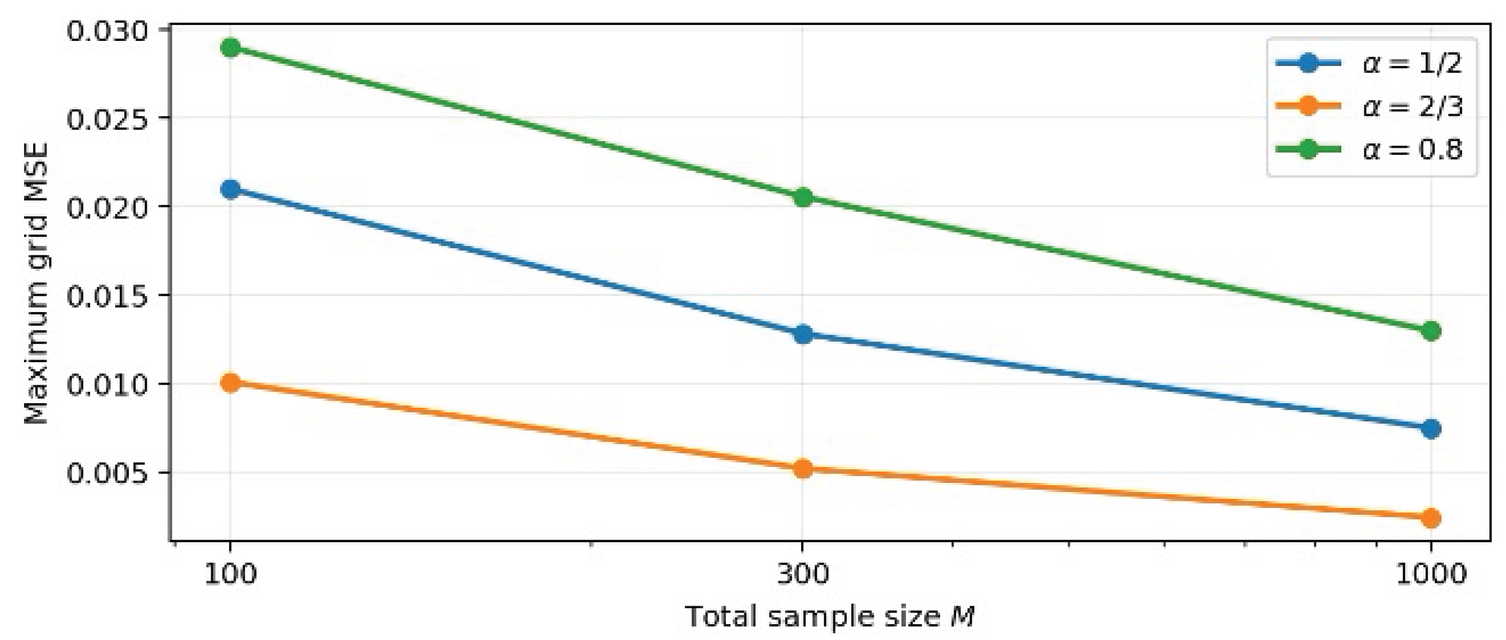

Table 1.
Simulated allocation MSE for the feasible two-stage rule.
| M | Pilot L | Max grid MSE | P at max | Mean grid MSE | |
|---|---|---|---|---|---|
| 100 | 10 | 0.021028 | 0.500 | 0.005748 | |
| 100 | 22 | 0.010108 | 0.500 | 0.004585 | |
| 100 | 40 | 0.029036 | 0.010 | 0.015205 | |
| 300 | 18 | 0.012841 | 0.500 | 0.003224 | |
| 300 | 46 | 0.005224 | 0.500 | 0.002279 | |
| 300 | 96 | 0.020583 | 0.990 | 0.009755 | |
| 1000 | 32 | 0.007514 | 0.500 | 0.001805 | |
| 1000 | 100 | 0.002456 | 0.500 | 0.000913 | |
| 1000 | 252 | 0.013005 | 0.010 | 0.005451 |
Table 2.
Practical interpretation of the four pilot-size regimes.
| Pilot choice | Pilot order | Dominant mechanism | MSE order | Practical reading |
|---|---|---|---|---|
| Square-root benchmark | Pilot estimation | Valid first-order pilot, but estimation remains comparatively slow. | ||
| Intermediate pilot | Pilot estimation | Increasing the pilot improves the worst-case rate. | ||
| Balanced rate | Pilot estimation = Stage-1 allocation | The two errors have the same order; this is the unique minimax-rate balance. | ||
| Oversized pilot | Stage-1 allocation effect | Additional pilot observations now worsen the worst-case rate because too much is committed early. |
Disclaimer/Publisher’s Note: The statements, opinions and data contained in all publications are solely those of the individual author(s) and contributor(s) and not of MDPI and/or the editor(s). MDPI and/or the editor(s) disclaim responsibility for any injury to people or property resulting from any ideas, methods, instructions or products referred to in the content. |
© 2026 by the authors. Licensee MDPI, Basel, Switzerland. This article is an open access article distributed under the terms and conditions of the Creative Commons Attribution (CC BY) license (http://creativecommons.org/licenses/by/4.0/).
Copyright: This open access article is published under a Creative Commons CC BY 4.0 license, which permit the free download, distribution, and reuse, provided that the author and preprint are cited in any reuse.