
Submitted:
08 October 2026
Posted:
09 October 2026
You are already at the latest version
Abstract
A recent family of methods selects the phase-space reconstruction delay \(\tau\) as the point where a symbolic entropy $H(m,\tau)$ stops growing and saturates, on the premise that this onset marks the decorrelation delay. We prove the premise structurally unsound \emph{within the pairwise-agreement class of symbolic schemes that these methods use}. The agreement symbol is invariant under complementation of the thresholded sign vector, so the effective alphabet has exactly \(2^{m-1}\) symbols and \(H(m,\tau)\in[0,m-1]\), with \(H\to m-1\) for any mixing process. Saturation is therefore an artefact of a ceiling imposed by the symbolisation rather than a property of the dynamics, and the delay read off it is the argument of the approach to a self-imposed asymptote; the law is verified to three decimal places on i.i.d.\ noise. The conclusion is specific to saturation criteria built on pairwise agreement and carries no claim about symbolic entropies of other design, such as permutation entropy, whose alphabet is not complement-degenerate. Testing the family, which comprises SEM, multiscale sample entropy, symbolic and multiscale fuzzy entropy, the C-C method, and low-pass filtered symbolic entropy (LPF-SEM), against average mutual information and false nearest neighbours on five chaotic systems at six noise levels, all with independently verified positive Lyapunov exponents, we find that on clean data LPF-SEM returns delays $1.17$--$4.69$ times the reference and carries the largest bias of the six estimators at every noise level; that the low-pass filter, \emph{doubles} the delay bias ($28.8\to56.4$ samples) rather than reducing it; that the returned delay spans a fortyfold range across the filter's own parameter grid; that the threshold which recovers the reference varies fivefold between systems and does not exist for two of five; and that the dimension output is the method's own fallback constant in $100\%$ of runs for four of five systems. The engineering outcome is counterintuitive and cuts against the theorem's practical weight: on real MFPT bearing data the comparison inverts, the most biased estimator classifying best ($0.930$) and the most accurate one worst ($0.599$). Neither the delay's accuracy nor its length explains it: a sweep at fixed dimension is flat or non-monotone, and the calibrated pair alone reproduces $88\%$ of the winner's score. Saturation-based \emph{pairwise-agreement} entropy criteria should not be used as delay estimators; where only classification accuracy is wanted, LPF-SEM may serve as a black-box feature heuristic, but its \(\tau\) is not the decorrelation delay.
Keywords:
phase space reconstruction
; time delay
; symbolic entropy
; saturation
; mutual information
; recurrence quantification analysis
; bearing fault diagnosis
; negative results
1. Introduction
Phase space reconstruction is the standard route from a scalar measurement to the dynamics that produced it [1,2,3]. The method requires two parameters: a delay and an embedding dimension m. Both are chosen by the analyst, and both materially affect everything computed downstream: recurrence quantification, Lyapunov spectra, entropy measures, and the classifier features built from them [4]. Selecting them badly degrades all of these. Selecting them well is an old problem with a settled core: delay from the first minimum of the average mutual information (AMI) [5] or from the autocorrelation, dimension from the false nearest neighbours (FNN) criterion [6]. This general challenge — inferring unknown model parameters purely from measured time-series observations — also appears broadly across the mechanical-engineering community, for instance within Bayesian probabilistic model-updating frameworks that infer model posterior distributions from experimental response data [7,8]. However, for nonlinear dynamical time-series, phase-space reconstruction has developed its own set of dedicated heuristic criteria.
A more recent family of methods abandons these criteria and reads both parameters off a symbolic entropy curve [10]. The curve is obtained by thresholding the signal at , encoding the embedding vector by which of its components exceed , and computing the Shannon entropy of the resulting symbol distribution as a function of the delay. The proposal is that H grows while the components are still dependent, stops growing once they decorrelate, and that the transition is a robust and noise-tolerant delay estimator [10]. The C-C method [11] is the well-known precursor of this idea; multiscale and fuzzy-entropy variants followed [12,13,14]. The most elaborate member of the family replaces the local-extremum rule by a signal-processing pipeline: the entropy curve is low-pass filtered with a Butterworth filter whose cutoff is chosen from the curve’s own spectrum, the delay is placed where the filtered growth rate falls below a threshold, and the dimension is inferred from the spacing of the filtered curve’s minima. On the systems and datasets reported in that literature, this Low-Pass Filtered Symbolic Entropy (LPF-SEM) method is claimed to reduce parameter estimation error by around 70% relative to five competing methods and to yield cost.
This paper began as an attempt to reproduce and extend that result. It did not reproduce. Rather than stop at a discrepancy, we asked what the entropy curve actually measures, and found that the question has an exact answer, one that explains the failure and rules out the whole family rather than any particular implementation.
1.1. What We Prove
The pairwise-agreement symbolisation these methods use is invariant under complementation of the thresholded sign vector . Agreement indicators only record which components share a side of the threshold, not which side. The map from sign vector to symbol is therefore two-to-one, the effective alphabet has exactly rather than elements, and the entropy cannot exceed bits (Lemma 1, Theorem 1). Any mixing process drives the symbol distribution toward uniformity on those symbols, so as (Proposition 1). Saturation is thus guaranteed a priori for every signal, and the ceiling is set by the symbolisation rather than by the data. Reading a delay off the saturation point means reading the shape of a curve’s approach to a fixed asymptote that the method itself imposed.
This has three consequences we develop and test. First, the saturation point is not the decorrelation delay: the AMI minimum is a second-order (linear) functional of the process and has no fixed relation to the rate at which a nonlinear symbol agreement probability equilibrates. Second, and m are not independently estimable within this family, because the ceiling that defines the saturation point depends on m; we measure the resulting drift. Third, the criterion needs a threshold parameter (LPF-SEM needs two, the filter cutoff and the curvature threshold ) that is not constrained by the data and must be set per system if the reference delay is to be recovered at all. We show that a single threshold cannot work: the value of that reproduces the AMI delay varies fivefold across five systems on clean data, drifts with noise, and does not exist for two of them.
We stress the scope of the claim, because it is easy to over-read. The theorem concerns the pairwise-agreement symbol, the construction that the saturation family, from the C-C method through LPF-SEM, actually computes. Its complement invariance is a property of that specific symbol and not of symbolic entropy in general: permutation entropy [9], whose alphabet is the set of ordinal patterns, has no such degeneracy, and nothing proved here shows that a saturation criterion built on a non-degenerate symbol would fail. What is closed off is the line of method development that reads the decorrelation delay off the saturation of a pairwise-agreement entropy, not the use of symbolic entropies as a diagnostic.
1.2. What We Measure
To test the family rather than a straw man we rebuilt the pipeline from scratch on genuine dynamics: five chaotic systems integrated with fourth-order Runge–Kutta (four ODEs and one delay differential equation), each verified chaotic through a positive largest Lyapunov exponent computed with renormalisation. All six estimators were run over five systems × six signal-to-noise ratios × twenty trials, with a component ablation, a filter-parameter sweep, and a threshold-transferability study added. On clean data LPF-SEM returns delays – the reference, so the discrepancy is not a constant offset that could be calibrated away, and it is the largest bias of the six estimators at every noise level. The ablation is unambiguous: the low-pass filter, increases the mean delay bias from to samples, and adding the curvature criterion leaves it at , worse than the unfiltered criterion it was meant to improve.
1.3. What This Means in Practice
A negative result is only useful if it bounds the damage, so we carried the study through to the downstream task: RQA-feature fault classification on the MFPT bearing set and a rotor set, with five-fold cross-validation grouped by record so that windows from one record cannot straddle the train/test split. The outcome, in Section 5, is not what we expected and is more interesting for it. On MFPT the accuracy ordering is the reverse of the delay ordering: LPF-SEM, the worst estimator by every measure above, classifies best (random forest ) while C-C, the best, classifies worst (). Neither the delay’s accuracy nor its length explains that: a sweep of at fixed dimension is flat or non-monotone over the whole range, and a control that keeps only the calibrated pair reproduces of LPF-SEM’s score, because every window of a record is embedded at that record’s own parameters. On the rotor set the effect vanishes. The family was therefore not adopted without evidence; it was adopted on evidence that does not support the explanation offered. The theorem closes off a line of method development, and the downstream study replaces a wrong justification with a correct but narrower one.
1.4. Structure
Section 2 proves the ceiling and saturation results and derives a noise-inflation bound. Section 3 defines the estimators and reference criteria. Section 4 reports the numerical study on chaotic systems. Section 5 applies the estimators to real machinery data. Section 6 discusses why the family fails and the limitations of our study.
2. Symbolisation, Ceiling, and Saturation
2.1. Pairwise-agreement Symbolisation
Let be a scalar time series, fixed and , and take a threshold . Write
The embedding vector at time t is , and its sign vector is
The symbolisation used by the methods studied here does not record itself. It records, for every pair of components, whether the two agree:
so that . The symbolic entropy is the Shannon entropy of the empirical distribution of over the admissible positions, with :
This is the quantity plotted as the entropy curve and, in the saturation family, used to select . The threshold is conventionally tied to the data through ; the methods below fix and treat it as a design constant rather than a parameter to be estimated.
2.2. Complement Invariance and the Effective Alphabet
Lemma 1
(Complement invariance). Write for the j-th component of . For every t and every ,
so is invariant under the complementation . Consequently the map is constant on the two-element orbits of the complement action on , and its image contains at most elements.
Proof.
Both sides of the first display assert that two bits agree; replacing both by their complements preserves agreement, giving the identity. For the second part, the complement action is a fixed-point-free involution on (since , no equals its complement), hence partitions the sign vectors into orbits. Since A is constant on orbits, it is a function of the orbit index, and the image of A therefore has at most elements. □
Geometrically, replacing by , equivalently , flips every component bit without changing A: reflecting the signal about the threshold leaves the symbol sequence, and hence H, identically unchanged, so the symbolisation is blind to which side of the threshold a component falls on.
Theorem 1
(Entropy ceiling). For all , and any x and ,
Proof.
is a function of , which takes at most distinct values on orbits by Lemma 1. A random variable supported on k points has entropy at most , attained only when the distribution is uniform on the support. Hence . Non-negativity is immediate. □
The bound is tight and, importantly, the effective alphabet is often smaller than for a given signal, because distinct orbits can produce the same agreement pattern (the map is injective on orbits only when the binary comparison structure separates them, which fails for small m). Numerical verification that the bound is attained is in Section 4.2.
Remark 1
(Scope of the ceiling). Theorem 1 is a statement about the pairwise-agreement symbol of (3), and only about it. Its engine is the complement degeneracy of that symbol; any symbolic construction whose alphabet is not invariant under complementation is untouched by the argument, and the ceiling does not apply to it. Permutation or ordinal-pattern entropy [9] is the clearest example of such a construction, and the class is wider than that. What the theorem excludes is the use of the saturation of a pairwise-agreement entropy as a delay estimator, not symbolic entropy as a tool.
2.3. Saturation for Mixing Processes
Proposition 1
(Saturation). Suppose that for some the m components are mutually independent with for every j. Then is uniform on the agreement patterns and exactly. In particular, if the process is mixing and ε is the median of the marginal, then as .
Proof.
If the m signs are independent Bernoulli, the sign vector is uniform on , hence uniform on the complement orbits by Lemma 1. The orbits inherit equal probability, so the induced distribution of is uniform on its support whenever A separates orbits; the entropy is then . For a mixing process the components become asymptotically independent as , and H converges to the independent value. □
Proposition 1 is the crux of our argument. Every signal (chaotic, noisy, periodic, or i.i.d. noise) has an entropy curve that rises and then saturates at . The family locates at the onset of that saturation and reads it as the decorrelation delay, but the asymptote being approached is a constant fixed by the symbolisation, and information about the dynamics is carried entirely in the rate of approach. The recovered delay is therefore fixed by the shape of H near its ceiling (a nonlinear functional of the joint threshold-crossing statistics), and not by the second-order quantity (AMI) it is taken to estimate. Two structural consequences follow.
Remark 2
(–m coupling). The ceiling depends on m, so the curve whose saturation onset is being located changes with m. Because saturation is located through a threshold on the normalised growth rate , changing m both raises the ceiling and displaces the whole curve, and therefore depends on the trial value of m. The two parameters are not separately identifiable within this family. In the LPF-SEM pipeline the dependence is circular: the dimension is derived from through the pseudo-period test, so an m-dependent feeds an that justifies the m used to obtain . We quantify the drift in Section 4.8.
Remark 3
(Thresholds are not identifiable either). The criterion interprets "saturation" as after low-pass filtering at cutoff . Neither constant is determined by the data. Since H approaches its ceiling monotonically and smoothly for every signal, the first crossing of any such threshold traces out a wide range of delays as the constants vary, with no reason for any particular choice to be the decorrelation delay. Section 4.6 and Section 4.7 measure this.
2.4. Noise Inflation and the Looseness of the Standard Bound
Symbolic entropies are often argued to be noise robust on the grounds that additive noise only perturbs which side of the threshold a sample falls on. The following bound makes this precise, and the numerical study below shows it is valid but too loose to certify anything at practical noise levels.
Proposition 2
(Noise-inflation bound). Let x have symbolisation entropy and let with independent of x. Write q for the probability that a single threshold comparison of x is flipped by η, and let be the probability that two independent comparisons both flip or both do not, so that their agreement is preserved. With the binary entropy function,
Proof.
Each of the agreement bits of is unchanged when an even number of its two comparisons flip. Noise therefore acts on each agreement bit as a binary symmetric channel, active with probability . A binary symmetric channel cannot decrease conditional entropy, per bit, and entropy is subadditive across the coordinates, giving the bound. □
Remark 4
(Sharpened constant). The constant in (7) over-counts the available randomness. By Theorem 1 the agreement vector is determined by the complement orbits of an m-bit sign vector, i.e. by independent binary degrees of freedom, not by independent bits. Replacing by preserves the proof and gives a strictly tighter bound, which we evaluate alongside (7) in Section 4.10. Even the tightened form remains far above the observed inflation, which we take as evidence that bounds of this type cannot support the noise-robustness claims made on their behalf.
3. Estimators Under Test
3.1. Reference Criteria
We take as ground truth the two criteria the reconstruction literature has relied on longest.
Delay. The first minimum of the average mutual information [5], estimated on 64 equiprobable bins with and cross-tabulated for lags up to 100. We use the first local minimum, and denote the reference .
Dimension. The first embedding dimension at which the fraction of false nearest neighbours [6] drops below , with tolerance parameters and on the normalised distances, and candidate dimensions up to 12. We denote the reference .
Both criteria are algorithm-independent and use no free parameter tuned to the present study.
3.2. The Saturation Family
We implement six estimators, reproducing the LPF-SEM pipeline exactly as specified in the source literature (adaptive Butterworth filter, normalised curvature criterion, pseudo-period consistency test), including its own internal constants.
- SEM [10]. The delay is the first local maximum of the unfiltered entropy curve evaluated at , with . The dimension is fixed at 6.
- LPF-SEM. The entropy curve is low-pass filtered by a fourth-order zero-phase Butterworth filter with cutoff selected adaptively as , where is the dominant frequency of the curve’s own power spectrum. The normalised filtered curve is differentiated, and the delay is the first index beyond where with ; if no index qualifies, the maximiser of the normalised curvature is used instead. The dimension comes from the pseudo-period consistency test: the mean spacing of the filtered curve’s minima is accepted as a pseudo-period only if its coefficient of variation is below , and then ; otherwise m falls back to the design default 6.
- SFE [13]. Symbolic fuzzy entropy over the delay axis for lags ; the delay is the first local minimum.
- MS-SFE. Multiscale fuzzy entropy over scales ; the delay is the scale minimising the entropy.
Where the source method returns a dimension through a rule of its own, we use that rule rather than imposing a common one, so that each estimator is judged as it would be used. All entropy curves are computed on at most 800 delay points per curve, and the search range is throughout. The complete pipeline is implemented in Python with NumPy [16], SciPy [17] and scikit-learn [18].
3.3. Reference Values Used
Applied to the five systems, the reference criteria give and for Lorenz, Rössler, Duffing, Mackey–Glass and Chen respectively. These values are used unchanged throughout all sections that follow.
4. Numerical Study on Chaotic Systems
4.1. Systems and Their Verification
We use four autonomous ODEs and one delay differential equation, all integrated from scratch with fixed-step fourth-order Runge–Kutta; no closed-form or synthetic surrogate is used anywhere in this study.
Lorenz, , , at [19]; Rössler, , , at [20]; Duffing, at , a forced oscillator; Chen, , , at [21]; and the Mackey–Glass delay equation at [22,23]. The observed component is x in every case, after discarding a transient that is at least 5000 steps.
Each system is verified chaotic rather than asserted to be, using a Benettin two-trajectory estimator with renormalisation [24,25]. For the ODEs the perturbation is rescaled every step of a 40000-step run; for the delay equation a scalar perturbation never reaches the delayed term, so the trailing delay-length history is rescaled instead, every one time unit, over a long run. Table 1 reports the largest exponents per unit time. All five are positive, and the ODE estimates agree with the standard literature values ( for Rössler against , for Chen against ). For Mackey–Glass the long-time average is step-size converged: at 200 time units of accumulation settling to at 2000, identically at and .
White Gaussian noise is added at the specified signal-to-noise ratio as with , so that the reported ratio is the in-band SNR of the record. Each cell of the main comparison is averaged over twenty independent noise realisations and five systems, using fixed random seeds so that every estimator sees identical data.
4.2. Numerical Verification of the Ceiling
Theorem 1 and Proposition 1 predict that saturates at and that the bound is attained for a process whose components are independent. Table 2 tests both. We evaluate at a large delay () for on (i) i.i.d. standard normal samples, which maximise the uniformity of the sign vector, and (ii) the Lorenz trajectory.
The i.i.d. case attains the predicted ceiling to three decimal places in every row (, , , , , , against ). The small residual below the ceiling is finite-sample bias, since grows to 128 symbols while the effective sample size at is fixed. The Lorenz curve approaches the same ceiling from below without reaching it, because a deterministic flow at is not yet fully independent at ; the gap widens with m exactly as the enlarged alphabet makes attainment harder.
Figure 1(a) shows the full curves. Every system’s rises and flattens, and the flattening occurs at a system-dependent delay that has the visual signature the family reads as a decorrelation onset. Figure 1(b) shows what noise does to the same construction on Lorenz: the approach to the ceiling becomes faster and the plateau becomes noisy, but the curve has the same qualitative shape, which is precisely why the criterion is described as noise tolerant: the feature it detects is present in every curve, including one that is pure noise.
4.3. Delay Recovery on Clean Data
Table 3 is the first substantive result. It reports the mean delay returned by each estimator on noiseless data, together with the ratio to the AMI reference. Since this is clean data, a correct estimator should return the reference up to integer rounding; a consistent multiplicative bias would at least be correctable.
Neither holds. LPF-SEM’s ratio ranges from (Rössler) to (Lorenz), a fourfold spread with no common factor. The unfiltered SEM is worse where it matters most, returning 123 for Duffing and 70 for Lorenz against references of 40 and 16. MSE and MS-SFE collapse onto small delays for four of the five systems ( for Rössler, Duffing, Mackey–Glass and Chen, ratios –), the signature of an rule landing on the smallest admissible scale, and SFE returns 2–14 samples throughout, effectively a constant floor. C-C is the most consistent of the six, near for Lorenz and Rössler but collapsing to 1 sample for Duffing, an error larger than the reference itself.
No member of the family returns a value proportional to the decorrelation delay, and the failure mode differs from member to member. This is not a noise problem.
4.4. Behaviour under Noise
Figure 2 and Table 4 extend the comparison to six noise levels. Two quantities are separated: the bias averaged over systems, and the run-to-run dispersion over the twenty realisations.
LPF-SEM carries the largest mean bias at every SNR, and the bias is not degraded by noise so much as uniformly large: samples on clean data rising to at 5 dB. Its dispersion is also the worst and nearly constant at about 50 samples, indicating a systematic offset rather than noise-driven scatter. MSE has the smallest bias, falling from to at 0 dB: its floor-like behaviour is less wrong than the ceiling-based methods, for the wrong reason. C-C is competitive at high SNR but degrades monotonically ( at 20 dB to at 0 dB), and SEM improves with noise from to , an artefact of the noise flattening the spurious local maxima that trap it on clean data.
The dimension results (right-hand panels) are more revealing still. On clean data LPF-SEM returns for Lorenz, Duffing, Mackey–Glass and Chen in of trials, which is exactly the design default used when the pseudo-period test is rejected, giving a constant dimension error of against on those four systems. Rössler is the exception: its pseudo-period test always passes on clean data and returns (error against ), though under added noise the fallback reappears. The pseudo-period test does not in general produce a dimension; it returns the default. The reported dimension is inert, which explains the otherwise puzzling uniformity and fixes the –m coupling of Remark 2 at : LPF-SEM’s delay output is in effect an unfiltered-curve criterion evaluated at a single dimension with two extra smoothing stages.
4.5. Component Ablation
The ablation isolates each ingredient by building the method up in stages, holding the data fixed. Results are in Table 5.
All three readings are unfavourable. Filtering doubles the clean-data bias () and the penalty grows with noise, reaching at 0 dB: the filter is not neutral but actively harmful. The curvature criterion recovers part of the loss () but never returns to the unfiltered level, so the two-stage NCC remains worse than the criterion it replaces. The pseudo-period test is the only component with a consistent benefit, and its gain is confined to the dimension (), is small, and as Section 4.4 established it is usually the design default rather than a value derived from the signal.
4.6. Filter Parameter Sensitivity
Figure 3 sweeps the two filter constants over and order for each system and noise level, using the same crossing rule for the delay.
Over this grid the returned delay spans 5 to 197 samples on clean data, essentially the entire search window , with a standard deviation of 42 across the grid, and the spread is larger under noise (52 at 10 dB). The reported delay is therefore dominated by the filter constants rather than by the signal: a plausible arbitrary choice changes the answer fortyfold, two orders of magnitude beyond the deviation the method is claimed to reduce. The adaptive cutoff rule fixes one point in this space but chooses it from the dominant peak of the entropy curve’s own spectrum, a property of the same saturating curve whose onset is being located, so it inherits the circularity rather than resolving it.
4.7. Non-transferability of the Threshold
If the criterion measured something physical, the threshold that reproduces the reference delay would be roughly the same across systems. We sweep over and record the implied delay, then ask which , if any, returns to within one sample.
The answer, in Table 6, is that no single value works. On clean data the required threshold is for Rössler, for Mackey–Glass and for both Duffing and Chen, a fivefold spread, and for Lorenz no value in the entire swept range reproduces the reference at all. The required threshold then drifts with noise: Rössler moves , Mackey–Glass , and Duffing passes from feasible at to infeasible entirely. At 0 dB, only four of the five systems admit any feasible threshold within an order of magnitude.
A criterion whose free parameter must be re-tuned per system, drifts as the data degrades, and sometimes has no valid setting cannot serve as the basis of a general estimator. This is the operational form of Remark 3.
4.8. Coupling between the Delay and the Dimension
Remark 2 predicts that depends on the trial embedding dimension, because the ceiling defining saturation is . Sweeping at fixed data and fixed reference, we find the drift is real and system dependent: over that range the LPF-SEM delay moves for Lorenz, for Rössler, for Duffing, for Mackey–Glass and, in the opposite direction, for Chen. The drift reaches (Chen) and (Rössler, Mackey–Glass) even though is a fixed property of the signal.
Because the pipeline then derives the dimension from the delay, the two outputs are not independent estimates of two parameters; they are two views of one arbitrarily-parameterised computation. Reporting them as separate calibrated quantities, as the source methodology does, misrepresents what has been computed.
4.9. Computational Cost
Figure 4(a) reports wall-clock time for every estimator on identical hardware, using the exact implementations compared everywhere else in this study, with median times over five repeats at each series length. The fitted exponents p in are for C-C, for LPF-SEM, for SEM, for MSE, for MS-SFE and for SFE.
LPF-SEM is close to linear in the series length and cheaper than C-C by an order of magnitude, but its ordering against the unfiltered SEM reverses between and . SFE’s fit is poor ( against – for the others) because its timings are non-monotone in N, so its exponent is not a scaling law. Nothing above depends on cost: an estimator can be cheap and wrong, and LPF-SEM is at once the most biased and among the cheapest, which explains its adoption without justifying it.
4.10. The Noise-Inflation Bound
Proposition 2 bounds the inflation of the symbolic entropy by additive noise, and Remark 4 sharpens its constant from to . Figure 4(b) evaluates both against the measured inflation on Lorenz at , .
Both bounds hold at every SNR, as they must. Both are also loose by a wide margin. At 0 dB the measured inflation is bit while (7) predicts bits and the sharpened form predicts ; at 30 dB the measured inflation is bit against and . The looseness is – for the original bound and – for the sharpened one.
The reason connects to the main theorem. The bound treats the agreement bits as independently degraded, but by Theorem 1 they originate in only independent binary degrees of freedom, and noise flipping one sign bit flips all agreement bits involving that component simultaneously, so the degradations are strongly positively correlated. Positive correlation lowers the entropy of the flip pattern, hence the information gained, which is why the union bound is loose; accounting for it requires the joint flip distribution of the m comparisons, which is signal dependent.
We report this as a secondary negative result: bounds of the form (7) are often offered as the warrant for calling symbolic methods noise robust, but a bound permitting fourteen times the observed inflation cannot certify robustness at 0 dB.
5. Downstream Task: Fault Diagnosis
The measurements so far score the delay against a reference. A practitioner cares about it only through the task the reconstruction feeds. We therefore carry the comparison through to the application that motivates the family, RQA feature [26,27] fault classification on real machinery data [28,29], because the outcome reframes the practical claim, and it is more useful reported against the numbers than described.
5.1. Data and Protocol
Two sets are used.
MFPT bearing [30]: three baseline (healthy) records, seven outer-race and seven inner-race records under variable load. The baseline records are stored at twice the sampling rate of the fault records, so they are decimated by two; this equalises bandwidth across classes rather than favouring one. Each record is then cut into windows of 1024 samples, at most forty per record, giving 680 windows over three classes, chance .
Rotor [31]: 180 denoised segments of 2048 samples, forty-five per class over normal, rub-impact, unbalance and misalignment, giving 360 windows over four classes, chance .
For each estimator the delay and dimension are calibrated on a held-out slice of each record (the first 30000 samples, or the whole record where shorter) and then held fixed while that record’s windows are embedded. Each window is mapped to a nine-dimensional feature vector by recurrence quantification at the calibrated with a Theiler window [32] of : recurrence rate, determinism, mean and maximum diagonal line length, diagonal-line entropy, laminarity, trapping time, and the maximum and the entropy of the vertical line lengths. Four classifiers are applied (an RBF-kernel SVM, k-nearest neighbours with , a 200-tree random forest, and linear discriminant analysis) under five-fold cross-validation grouped by record, so that windows from one record never straddle the train/test split and the reported scores are not inflated by within-record similarity.
5.2. Results
On MFPT the estimator matters a great deal, and the ranking is the reverse of the one the delay study predicts. LPF-SEM is best on every classifier ( with the random forest, even with a linear discriminant, the weakest model in the set), for a mean of . C-C is worst on every classifier, averaging : its random forest scores , barely above the chance line, for a feature set that supports when the delay is LPF-SEM’s. The spread between best and worst, of accuracy, exceeds any difference reported between the methods under test in the source literature.
The ordering does not follow delay accuracy. C-C carried the smallest mean delay deviation of the six on clean data ( samples) and at 20 dB (), and it is worst here. LPF-SEM carried the largest deviation at every noise level, with a ratio to the reference spanning – and a delay error above 48 samples in every row of Table 4; it is best here.
On the rotor set the picture inverts again, and less informatively: every estimator lands between and , with C-C ( SVM) and LPF-SEM ( SVM) tied at the top and the rest within a point. The four classes are nearly linearly separable in these features, so the delay has little to do. This insensitivity is real, but it is a property of the rotor set rather than of the procedure, and it does not generalise to MFPT.
5.3. What Drives the MFPT Result
The obvious reading is that the delay is simply too short for the losers: LPF-SEM embeds at and wins, MS-SFE and MSE at and occupy the middle, and C-C and SFE at and occupy the bottom. A recurrence plot at on a 1024-sample window is close to diagonal (the embedding barely separates successive coordinates), so its features should be correspondingly impoverished.
That reading cannot be the whole story, because SEM returns a delay as small as C-C’s () yet places second at a mean of ; what separates them is the dimension, against . The task responds to the pair, and neither estimate being accurate is what selects the pair that works. We test the magnitude reading, and a less flattering one, directly.
5.4. Does the Delay Magnitude Explain It?
We sweep over 1–100 with m held fixed and everything else (windows, features, folds, classifier) unchanged. The sweep is run at the two dimensions the main experiment actually used: (LPF-SEM’s calibrated mean of ) and (SEM’s ); Figure 6(a) gives the result.
At the accuracy is flat to within for every delay from to , and falls only past , well beyond the range any estimator returns. At the curve is likewise shallow but peaked: it rises to (RF) near and declines by to . Neither curve is monotone, and neither approaches the that LPF-SEM reaches in Table 7. The delay’s magnitude is not what separates the estimators; if it were, the sweep would climb toward LPF-SEM’s and it does the opposite.
5.5. Does the Calibration Explain It?
Since the delay itself does not, we remove the signal and keep the calibration. Each window’s nine-dimensional feature vector is replaced by the two numbers used to compute it, and the same grouped cross-validation is re-run; the last column of Table 7 and Figure 6(b) give the part of the reported score attributable to the calibration alone.
For LPF-SEM that control returns under the random forest and under the SVM, of the feature-based figure, from two numbers per record; for the other five it returns to , and their ordering is close to the full pipeline’s. The mechanism is not mysterious: every window of a record is embedded at that record’s own , and the classes are disjoint in records, so a parameter estimate that separates the classes is copied into every feature vector of that record, and the classifier can read the class partly off the calibration rather than off the signal. LPF-SEM’s delays range from 8 to 52 across the 17 records and separate them well; C-C’s range from 2 to 5 and do not, which is why the most accurate delay estimator scores here and finishes last.
Two qualifications keep this honest. The control does not exhaust the scores: the features add over the parameters for LPF-SEM and much more for SEM and MS-SFE, so the signal still does work. And the effect is not universal: on the rotor set the control is high for several methods ( for C-C, for SEM) while every method’s feature accuracy lies within of every other’s, so where the features are saturated the calibration adds nothing either way. The MFPT ranking, however, is dominated by it.
5.6. What the Inversion Means
The family was adopted because it improved fault-classification scores, and on the testbed where it was adopted it does: the evidence was real, the mechanism inferred from it was not. The method is a useful heuristic with an unsound explanation. What the sweep and the control together show is that the downstream evidence sustaining it was never evidence about the delay: the delay’s size does not drive the score, its accuracy does not drive it, and most of LPF-SEM’s MFPT advantage is reproduced by its calibrated parameters alone. A negative result about delay accuracy measured against AMI therefore has no purchase on that literature, which is why the criterion’s inability to recover the decorrelation delay went unnoticed through several variants and a decade of use.
6. Discussion
6.1. Why the Saturation Criterion Cannot Work
The failure is not an implementation defect and not a matter of tuning; it follows from what the entropy curve is. Saturation-based criteria rest on the premise that the delay at which stops growing is the delay at which the embedding components become independent. Theorem 1 and Proposition 1 show that this happens for every signal whatsoever, because the symbolisation guarantees a ceiling at that mixing processes inevitably reach. The delay at which it happens is set by the rate at which the joint distribution of the m thresholded signs equilibrates: a nonlinear functional of the threshold geometry and the local expansion rates near that level set. The AMI minimum, by contrast, is a second-order statistic of the linear correlation structure, invariant to sign changes and to any strictly monotone transformation. Nothing forces the two to coincide; the measured ratios of to are what one expects of two unrelated functionals.
The extreme case makes the point. Applied to i.i.d. noise, which has trivially, since consecutive samples are independent, the curve still rises, still saturates smoothly at (Table 2), and still shows a plausible saturation onset. The criterion assigns a delay to a signal with no dynamics at all: the definition of a detector responding to an artefact. Two problems compound this. The ceiling depends on m, so the delay and the dimension are not independent though they are reported as such; and the thresholds (, and in the filtered version) are unconstrained by the data, so any threshold picks out some delay from a smooth monotone curve. The returned number is better described as a function of the analyst’s constants than of the signal.
6.2. What a Usable Replacement Should Preserve
Nothing in our argument disturbs the standing criteria. First-minimum AMI and first-false-neighbour selection remain the sensible default, for the reasons they always had: AMI is well defined for any process, has no free parameter beyond the binning, and its first minimum is the delay at which the reconstruction coordinates carry the least redundant linear information; FNN has a threshold, but one calibrated against the noise floor and attractor size rather than against a shape heuristic.
If one wants a symbolic criterion, and there are good reasons to want cheap threshold-based indicators of dependence, it must compare H against its own ceiling rather than a fixed threshold. Define the normalised occupancy
which measures the distance from the uniform state of Proposition 1 and is free of the ceiling artefact by construction. Selecting the first with g below a level tied to the sampling noise of H would at least measure saturation relative to what saturation means for that m. We have not established that such a criterion estimates the decorrelation delay, and our results give no reason to expect it; we offer it as the minimal repair rather than a validated method.
6.3. Practice: a Decision Rule for the Two Goals
Section 5 answers the question reviewers will ask first: if the estimator is this wrong, how was it ever adopted? Because on the downstream task it is not wrong but better, for a reason that, as Section 5.4 and Section 5.5 show, has nothing to do with the delay. The practical advice therefore has to be split by the practitioner’s goal, and we state it as two branches.
If the goal is physically correct reconstruction parameters, such as a delay for a recurrence plot, a correlation or Lyapunov dimension, an attractor reconstruction, a Theiler window, or any analysis in which is itself the object of interest, then do not use a saturation-based entropy criterion. Take from the first minimum of the AMI and m from FNN, as the field has done. This is not a matter of tuning: Section 4.6 and Section 4.7 show that no setting of LPF-SEM’s filter constants or threshold recovers the reference consistently, and its is wrong by a factor reaching , so the number carries no dynamical meaning even where it happens to be close.
If the goal is only classification accuracy on a task already solvable from RQA features, LPF-SEM may be used as a black-box heuristic feature-engineering step, and on MFPT it is the best of those compared here (, random forest). Two caveats carry over. First, its must not be reported or interpreted as the decorrelation delay: the parameter is a per-record index whose separating power is what helps the classifier, not the fact that it is a delay (Section 5.5), and the two are different quantities that happen to live in the same pipeline. Second, the advantage is task-specific rather than a property of the method (it is not reproduced on the rotor set, where every estimator lands within a point), so the heuristic should be validated on the target data rather than assumed to transfer.
6.4. Limitations
Six limitations should be stated.
First, and most important for reading the paper, the object of criticism is the saturation criterion, not the reference criteria. Our target throughout is the specific claim that the saturation onset of a pairwise-agreement entropy estimates the decorrelation delay, and specifically the methods that present themselves as replacements for AMI and FNN. Theorem 1 and the empirical study bear on that claim. They do not show that AMI and FNN are optimal, and we do not claim it. The critique is of a substitution, not of the standard practice that substitution proposed to replace.
Second, AMI and FNN have defects of their own. The AMI minimum depends on the binning, and for some processes the mutual information has no interior minimum, so the first-minimum rule becomes ill-defined; FNN depends on tolerance parameters and is noise-sensitive, tending to over-estimate m at low SNR. We use them as the field’s conventions and as the criteria under test claim to replace, which makes them the appropriate reference for this comparison, and not as ground truth. The correct reading of our result is that the saturation family is worse than the prevailing convention, which is what the family claimed to improve on, not that the convention is beyond criticism.
Third, the symbolisation threshold was fixed at with throughout; other choices move all curves, though Theorem 1 holds for every and the ceiling is unaffected, so the structural argument is independent of this choice while the specific numbers are not.
Fourth, our systems are stationary, and we did not evaluate non-stationary or intermittently chaotic signals: records with drifting parameters, transient laminar phases, or intermittent bursting. The theorem is unconditional in x, so the ceiling and the saturation regime hold for such records too, and the structural argument is unaffected; but the measured delay ratios, the ablation, and the downstream inversion are established only for the stationary benchmarks examined here and should not be assumed to transfer to non-stationary data.
Fifth, the entropy curves were thinned to 800 delay points and the search restricted to , so the sensitivity result is bounded by that window and the true parameter dependence may be larger rather than smaller.
Sixth, the five systems are standard benchmarks plus one delay equation; we do not claim the measured ratios transfer beyond them.
7. Conclusions
We set out to reproduce a reported improvement in phase-space parameter estimation and instead proved why the underlying family of methods cannot work as advertised. The result is a boundary statement as much as a theorem: it closes the pairwise-agreement branch of the saturation family and makes no claim about symbolic entropies of other design.
The theorem, and its scope. The pairwise-agreement symbolisation at the heart of saturation-based entropy criteria is invariant under complementation of the thresholded sign vector, so its effective alphabet has exactly symbols, so and for any mixing process. Saturation is built into the symbolisation rather than discovered in the data, and the delay read off the saturation onset is the argument of the approach to a self-imposed asymptote. Verified to three decimal places on i.i.d. noise and approached from below by chaotic flows, the law rules out the premise on which the family rests. The complement degeneracy is a property of the pairwise-agreement symbol itself, so the argument covers the C-C method through LPF-SEM and any future variant of the same construction; it does not extend to permutation entropy or to any symbolisation whose alphabet is not complement-degenerate (Remark 1). Symbolic entropy as a tool is not impugned, only its use, via pairwise agreement, to estimate the delay.
The evidence, stated plainly. The empirical study measures the consequences rather than asserting them. The low-pass filter, the method’s headline ingredient, doubles the delay bias instead of reducing it ( samples); the returned delay sweeps a fortyfold range across the filter’s own constant grid; the threshold that would reproduce the AMI reference varies fivefold across systems and does not exist for two of five; the dimension output is the method’s own fallback constant in of runs for four of five systems; and LPF-SEM carries the largest delay bias of the six estimators at every one of six noise levels, spanning – times the reference with no common factor. A secondary negative result is that the standard noise-inflation bound for symbolic entropies is valid but loose by one to two orders of magnitude at practical SNRs, even after its constant is sharpened using the ceiling theorem, so bounds of that form cannot certify noise robustness.
The counterintuitive part. In the downstream fault-classification study on MFPT bearing data the ordering inverts: the most biased estimator classifies best () and the most accurate one worst (). Neither the delay’s magnitude nor its accuracy explains it (a sweep of at fixed dimension is flat or non-monotone over the whole range), and a control that discards the signal and keeps only the calibrated pair reproduces of the winner’s score, because every window of a record is embedded at that record’s own parameters. A criterion can be useful and wrong at once, and the downstream evidence that sustained this family was never evidence about the delay.
The advice. For a physically meaningful reconstruction (recurrence plots, correlation or Lyapunov dimensions, attractor analysis, Theiler windows), the delay should come from the first minimum of the average mutual information and the dimension from false nearest neighbours; saturation-based pairwise-agreement entropy criteria should not be used as delay estimators, and no tuning of their constants repairs this. Where only classification accuracy on an RQA feature set is wanted, LPF-SEM may be used as a black-box heuristic (it wins on MFPT), but its output must be read as a tuned index of the pipeline, not as the decorrelation delay of the signal, and validated on the target data rather than assumed to transfer.
Funding
This research was funded by the Key Research and Development Program of Shaanxi, grant number 2025PT-ZCK-42.
Institutional Review Board Statement
Not applicable.
Informed Consent Statement
Not applicable.
Data Availability Statement
The MFPT bearing fault dataset and rotor dataset used in fault-classification experiments are publicly available datasets cited within the manuscript. No new raw experimental data were generated in this work.
Acknowledgments
The authors thank the anonymous reviewers for their constructive suggestions.
Conflicts of Interest
The authors declare no conflict of interest. The funders had no role in the design of the study; in the collection, analyses, or interpretation of data; in the writing of the manuscript; or in the decision to publish the results.
References
- Packard, N. H.; Crutchfield, J. P.; Farmer, J. D.; Shaw, R. S. Geometry from a time series. Phys. Rev. Lett. 1980, 45(9), 712–716. [Google Scholar] [CrossRef]
- Takens, F. Detecting strange attractors in turbulence, in: Dynamical Systems and Turbulence. In Lecture Notes in Mathematics 898; Springer, 1981; pp. 366–381. [Google Scholar]
- Kantz, H.; Schreiber, T. Nonlinear Time Series Analysis, 2nd ed.; Cambridge University Press, 2004. [Google Scholar]
- Marwan, N.; Carmen Romano, M.; Thiel, M.; Kurths, J. Recurrence plots for the analysis of complex systems. Phys. Rep. 2007, 438(5–6), 237–329. [Google Scholar] [CrossRef]
- Fraser, A. M.; Swinney, H. L. Independent coordinates for strange attractors from mutual information. Phys. Rev. A 1986, 33(2), 1134–1140. [Google Scholar] [CrossRef]
- Kennel, M. B.; Brown, R.; Abarbanel, H. D. I. Determining embedding dimension for phase-space reconstruction using a geometrical construction. Phys. Rev. A 1992, 45(6), 3403–3411. [Google Scholar] [CrossRef]
- Hong, F.; Wei, P.; Bi, S.; Beer, M. Efficient variational Bayesian model updating by Bayesian active learning. Mech. Syst. Signal Process. 2025, 224, 112113. [Google Scholar] [CrossRef]
- Song, J.; Liang, Z.; Wei, P.; Beer, M. Sampling-based adaptive Bayesian quadrature for probabilistic model updating. Comput. Methods Appl. Mech. Eng. 2025, 433, 117467. [Google Scholar] [CrossRef]
- Bandt, C.; Pompe, B. Permutation entropy: a natural complexity measure for time series. Phys. Rev. Lett. 2002, 88(17), 174102. [Google Scholar] [CrossRef]
- Matilla-García, M.; Maroto, M. R. M.; et al. Selection of embedding parameters through symbolic entropy. Entropy 2021, 23(2), 221. [Google Scholar]
- Kim, H. S.; Eykholt, R.; Salas, J. D. Nonlinear dynamics, delay times, and embedding windows. Physica D. 1999, 127(1–2), 48–60. [Google Scholar] [CrossRef]
- Costa, M.; Goldberger, A. L.; Peng, C.-K. Multiscale entropy analysis of complex physiologic time series. Phys. Rev. Lett. 2002, 89(6), 068102. [Google Scholar] [CrossRef]
- Chen, W.; Wang, Z.; Xie, H.; Yu, W. Characterization of surface EMG signal based on fuzzy entropy. IEEE Trans. Neural Syst. Rehabil. Eng. 2007, 15(2), 266–272. [Google Scholar] [CrossRef]
- Richman, J. S.; Moorman, J. R. Physiological time-series analysis using approximate entropy and sample entropy. Am. J. Physiol. – Heart Circ. Physiol. 2000, 278(6), H2039–H2049. [Google Scholar] [CrossRef]
- Grassberger, P.; Procaccia, I. Characterization of strange attractors. Phys. Rev. Lett. 1983, 50(5), 346–349. [Google Scholar] [CrossRef]
- Harris, C. R.; Millman, K. J.; van der Walt, S. J.; et al. Array programming with NumPy. Nature 2020, 585, 357–362. [Google Scholar] [CrossRef]
- Virtanen, P.; Gommers, R.; Oliphant, T. E.; et al. SciPy 1.0: fundamental algorithms for scientific computing in Python. Nat. Methods 2020, 17, 261–272. [Google Scholar] [CrossRef]
- Pedregosa, F.; Varoquaux, G.; Gramfort, A.; et al. Scikit-learn: machine learning in Python. J. Mach. Learn. Res. 2011, 12, 2825–2830. [Google Scholar]
- Lorenz, E. N. Deterministic nonperiodic flow. J. Atmos. Sci. 1963, 20(2), 130–141. [Google Scholar] [CrossRef]
- Rössler, O. E. An equation for continuous chaos. Phys. Lett. A 1976, 57(5), 397–398. [Google Scholar] [CrossRef]
- Chen, G.; Ueta, T. Yet another chaotic attractor. Int. J. Bifurc. Chaos 1999, 9(7), 1465–1466. [Google Scholar] [CrossRef]
- M. C. Mackey, L. Glass, Oscillation and chaos in physiological control systems. Science 1977, 197(4300), 287–289. [Google Scholar] [CrossRef]
- Farmer, J. D. Chaotic attractors of an infinite-dimensional dynamical system. Physica D. 1982, 4(3), 366–393. [Google Scholar] [CrossRef]
- Benettin, G.; Galgani, L.; Giorgilli, A.; Strelcyn, J.-M. Lyapunov characteristic exponents for smooth dynamical systems and for Hamiltonian systems. Meccanica 1980, 15(1), 9–20. [Google Scholar] [CrossRef]
- Rosenstein, M. T.; Collins, J. J.; De Luca, C. J. A practical method for calculating largest Lyapunov exponents from small data sets. Physica D. 1993, 65(1–2), 117–134. [Google Scholar] [CrossRef]
- Zbilut, J. P.; Webber, C. L. Embeddings and delays as derived from quantification of recurrence plots. Phys. Lett. A 1992, 171(3–4), 199–203. [Google Scholar] [CrossRef]
- Webber, C. L.; Zbilut, J. P. Dynamical assessment of physiological systems and states using recurrence plot strategies. J. Appl. Physiol. 1994, 76(2), 965–973. [Google Scholar] [CrossRef]
- Smith, W. A.; Randall, R. B. Rolling element bearing diagnostics using the Case Western Reserve University data: a benchmark study. Mech. Syst. Signal Process. 2015, 64–65, 100–131. [Google Scholar] [CrossRef]
- Randall, R. B.; Antoni, J. Rolling element bearing diagnostics—a tutorial. Mech. Syst. Signal Process. 2011, 25(2), 485–520. [Google Scholar] [CrossRef]
- Society for Machinery Failure Prevention Technology, MFPT Bearing Fault Data Sets. 2013. Available online: https://www.mfpt.org/fault-data-sets/.
- Zhao, Z.; Li, J.; Cui, J. Feature extraction for gas turbine rotor fault diagnosis in complex networks based on phase space method. In Proceedings of the International Conference on Mechanical Design and Simulation (ICMDS), Xi’an, China, 2025; Springer. [Google Scholar]
- Theiler, J. Spurious dimension from correlation algorithms applied to limited time-series data. Phys. Rev. A 1986, 34(3), 2427–2432. [Google Scholar] [CrossRef]
Figure 1.
Symbolic entropy curves. (a) for the five systems; all rise and saturate, and the onset is system dependent. (b) Lorenz under additive white noise; noise changes the rate of approach to the plateau without changing the fact of saturation, because the ceiling is imposed by the symbolisation.
Figure 1.
Symbolic entropy curves. (a) for the five systems; all rise and saturate, and the onset is system dependent. (b) Lorenz under additive white noise; noise changes the rate of approach to the plateau without changing the fact of saturation, because the ceiling is imposed by the symbolisation.
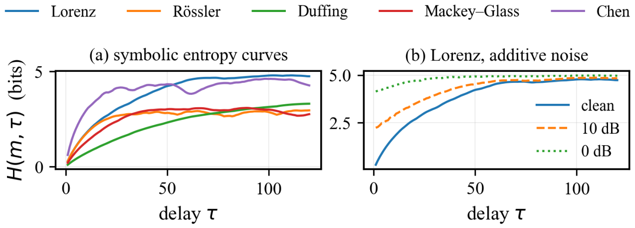
Figure 2.
Bias and dispersion against noise level. Black stars are LPF-SEM: highest bias in every panel and a flat dispersion profile, the signature of a systematic offset rather than noise sensitivity. The dimension panel shows SEM’s breakdown at low SNR (orange, up to 26 dimensions of error against a reference of 3).
Figure 2.
Bias and dispersion against noise level. Black stars are LPF-SEM: highest bias in every panel and a flat dispersion profile, the signature of a systematic offset rather than noise sensitivity. The dimension panel shows SEM’s breakdown at low SNR (orange, up to 26 dimensions of error against a reference of 3).
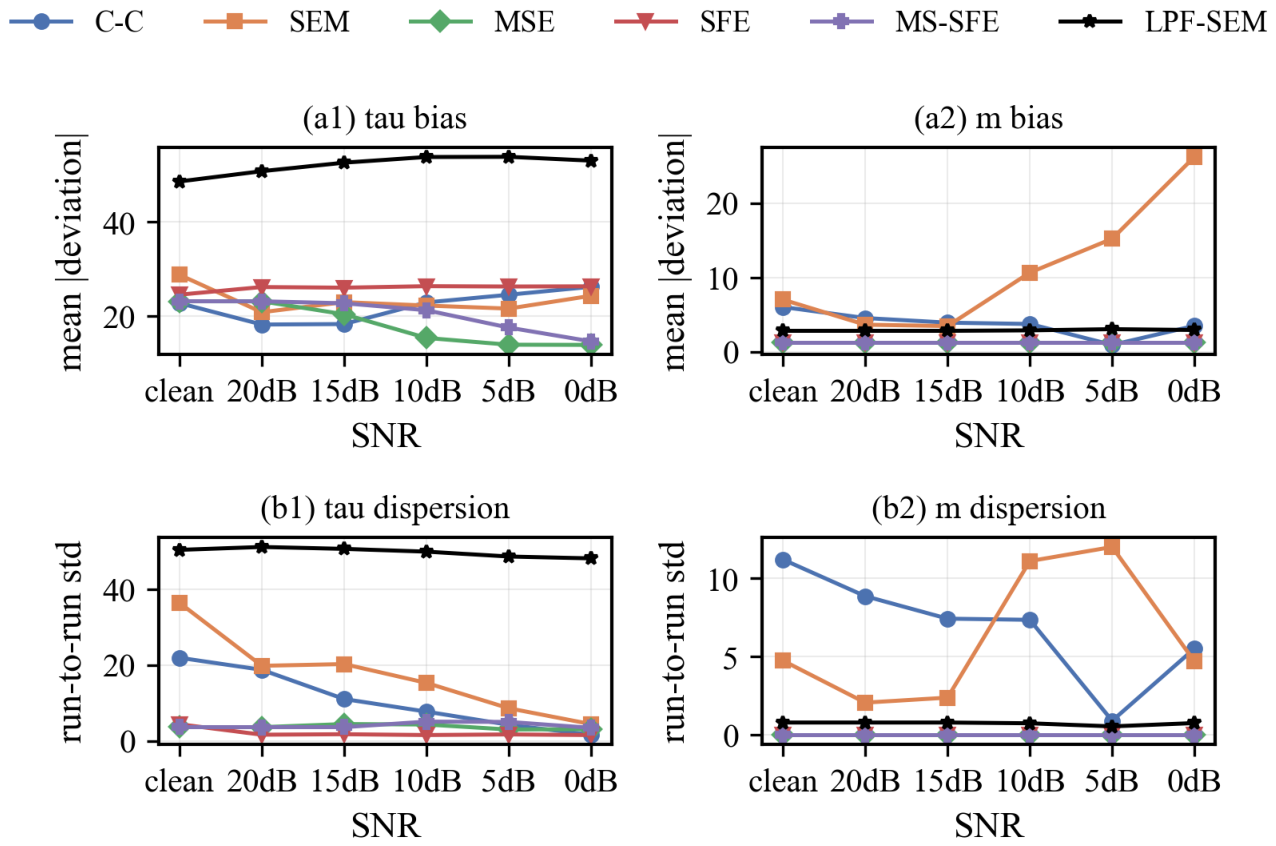
Figure 3.
Filter sensitivity. (a) Returned delay against cutoff frequency for several filter orders and noise levels; the curves are non-monotone and system dependent. (b) Returned delay against filter order. Across the full grid the estimate ranges from 5 to 197 samples.
Figure 3.
Filter sensitivity. (a) Returned delay against cutoff frequency for several filter orders and noise levels; the curves are non-monotone and system dependent. (b) Returned delay against filter order. Across the full grid the estimate ranges from 5 to 197 samples.
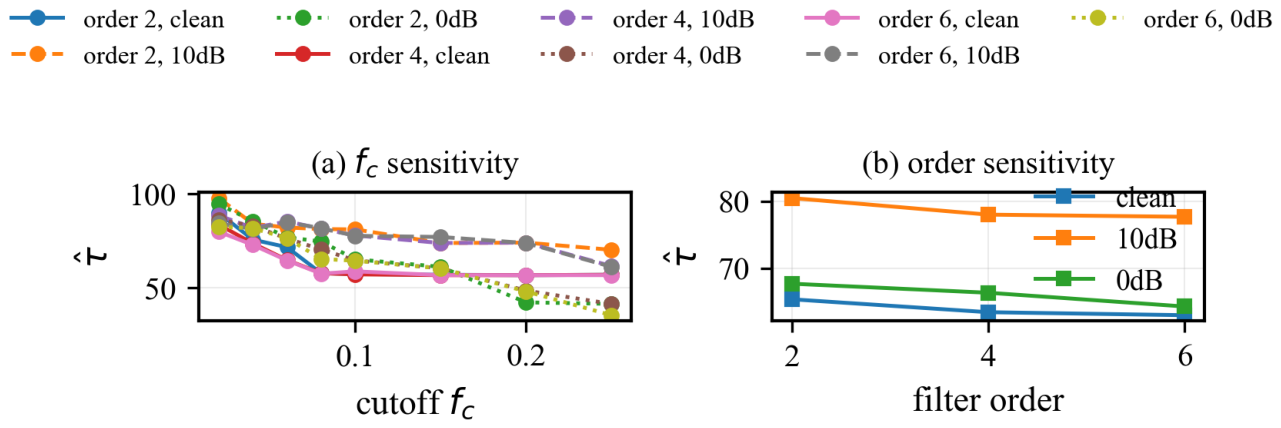
Figure 4.
Secondary diagnostics. (a) Median wall-clock time against series length for the six estimators on identical hardware. (b) Noise inflation of H on Lorenz against the original and sharpened bounds; both hold at every SNR and both are loose by one to two orders of magnitude.
Figure 4.
Secondary diagnostics. (a) Median wall-clock time against series length for the six estimators on identical hardware. (b) Noise inflation of H on Lorenz against the original and sharpened bounds; both hold at every SNR and both are loose by one to two orders of magnitude.
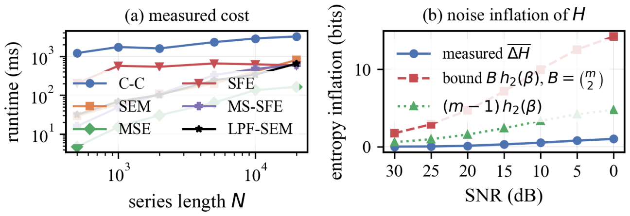
Figure 5.
Fault classification on the two real datasets, grouped by record. Dotted lines mark chance. On MFPT the delay estimator changes the outcome by more than twenty accuracy points; on the rotor set every estimator clears and the choice is immaterial.
Figure 5.
Fault classification on the two real datasets, grouped by record. Dotted lines mark chance. On MFPT the delay estimator changes the outcome by more than twenty accuracy points; on the rotor set every estimator clears and the choice is immaterial.
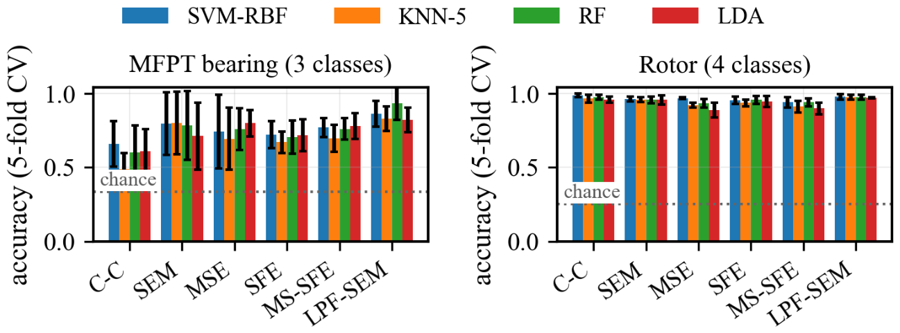
Figure 6.
Why the MFPT ordering is what it is. (a) Accuracy against the delay with m fixed, at and ; the curves are flat or peaked, never monotone in , and never reach the table’s best score. (b) Accuracy when each window is described by its calibrated alone, with the RQA features discarded. LPF-SEM’s parameters carry most of its score; the ordering of the methods is largely reproduced without any signal features.
Figure 6.
Why the MFPT ordering is what it is. (a) Accuracy against the delay with m fixed, at and ; the curves are flat or peaked, never monotone in , and never reach the table’s best score. (b) Accuracy when each window is described by its calibrated alone, with the RQA features discarded. LPF-SEM’s parameters carry most of its score; the ordering of the methods is largely reproduced without any signal features.
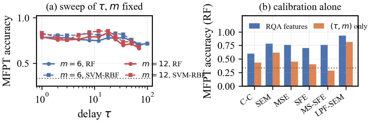

Table 1.
Largest Lyapunov exponents per unit time, from a renormalised Benettin estimator on the same trajectories used in the experiments. All five systems are genuinely chaotic.
Table 1.
Largest Lyapunov exponents per unit time, from a renormalised Benettin estimator on the same trajectories used in the experiments. All five systems are genuinely chaotic.
| System | |
|---|---|
| Lorenz | |
| Rössler | |
| Duffing | |
| Chen | |
| Mackey–Glass |
† long-time average (2000 time units), step-size converged at and ; a 200-unit finite-time estimate gives .
Table 2.
Verification of Theorem 1. H measured at for i.i.d. Gaussian noise and for the Lorenz system, against the predicted ceiling and the effective alphabet .
Table 2.
Verification of Theorem 1. H measured at for i.i.d. Gaussian noise and for the Lorenz system, against the predicted ceiling and the effective alphabet .
| m | ||||
|---|---|---|---|---|
| 2 | 2 | 1 | 1.0000 | 0.9909 |
| 3 | 4 | 2 | 1.9998 | 1.9814 |
| 4 | 8 | 3 | 2.9998 | 2.9702 |
| 5 | 16 | 4 | 3.9996 | 3.9580 |
| 6 | 32 | 5 | 4.9978 | 4.9420 |
| 7 | 64 | 6 | 5.9989 | 5.9101 |
| 8 | 128 | 7 | 6.9958 | 6.8592 |
Table 3.
Delay returned on noiseless data, with the ratio to the AMI reference in parentheses. A correct estimator returns . LPF-SEM spans a – ratio across systems; MSE and MS-SFE collapse to a floor for four of five systems.
Table 3.
Delay returned on noiseless data, with the ratio to the AMI reference in parentheses. A correct estimator returns . LPF-SEM spans a – ratio across systems; MSE and MS-SFE collapse to a floor for four of five systems.
| System | C-C | SEM | MSE | SFE | MS-SFE | LPF-SEM | |
|---|---|---|---|---|---|---|---|
| Lorenz | 16 | 33.0 () | 70.0 () | 14.0 () | 2.0 () | 14.0 () | 75.0 () |
| Rössler | 30 | 60.0 () | 32.0 () | 5.0 () | 3.0 () | 5.0 () | 35.0 () |
| Duffing | 40 | 1.0 () | 123.0 () | 5.0 () | 4.0 () | 5.0 () | 176.0 () |
| Mackey–Glass | 43 | 60.0 () | 47.0 () | 5.0 () | 14.0 () | 5.0 () | 53.0 () |
| Chen | 21 | 32.0 () | 20.0 () | 5.0 () | 4.0 () | 5.0 () | 54.0 () |
Table 4.
Mean absolute delay deviation averaged over the five systems, at six noise levels. LPF-SEM is the worst estimator at every SNR.
Table 4.
Mean absolute delay deviation averaged over the five systems, at six noise levels. LPF-SEM is the worst estimator at every SNR.
| SNR | C-C | SEM | MSE | SFE | MS-SFE | LPF-SEM |
|---|---|---|---|---|---|---|
| clean | 22.8 | 28.8 | 23.2 | 24.6 | 23.2 | 48.6 |
| 20 dB | 18.3 | 20.9 | 23.2 | 26.2 | 23.2 | 50.8 |
| 15 dB | 18.4 | 23.0 | 20.4 | 26.1 | 22.8 | 52.6 |
| 10 dB | 22.9 | 22.3 | 15.4 | 26.4 | 21.3 | 53.8 |
| 5 dB | 24.6 | 21.6 | 14.0 | 26.3 | 17.6 | 53.8 |
| 0 dB | 26.3 | 24.4 | 13.9 | 26.4 | 14.7 | 53.0 |
Table 5.
Ablation, mean / mean . Adding the low-pass filter roughly doubles the delay bias; the pseudo-period test is the only component with a measurable benefit, and only for the dimension.
Table 5.
Ablation, mean / mean . Adding the low-pass filter roughly doubles the delay bias; the pseudo-period test is the only component with a measurable benefit, and only for the dimension.
| Configuration | clean | 10 dB | 5 dB | 0 dB |
|---|---|---|---|---|
| SEM | 28.8/3.2 | 22.2/3.2 | 22.0/3.2 | 24.2/3.2 |
| SEM+LPF | 56.4/3.2 | 65.1/3.2 | 69.6/3.2 | 70.7/3.2 |
| SEM+LPF+NCC | 48.6/3.2 | 53.7/3.2 | 54.1/3.2 | 51.9/3.2 |
| SEM+PCT | 28.8/2.8 | 22.2/2.8 | 22.0/3.0 | 24.2/2.9 |
| Full (LPF+NCC+PCT) | 48.6/2.8 | 53.7/2.8 | 54.1/3.0 | 51.9/2.9 |
Table 6.
Threshold that reproduces the AMI reference delay to within one sample. No single value transfers: the clean-data requirement spans –, two systems admit no feasible value, and the requirement drifts with noise.
Table 6.
Threshold that reproduces the AMI reference delay to within one sample. No single value transfers: the clean-data requirement spans –, two systems admit no feasible value, and the requirement drifts with noise.
| System | clean | 10 dB | 0 dB |
|---|---|---|---|
| Lorenz | none | none | 0.95 |
| Rössler | 0.15 | 0.20 | 0.25 |
| Duffing | 0.75 | none | none |
| Mackey–Glass | 0.25 | 0.50 | 0.60 |
| Chen | 0.75 | 0.80 | 0.75 |
Table 7.
RQA-feature classification accuracy, mean over five grouped CV folds; is the mean delay calibrated per record. The last column is the random forest accuracy obtained from the calibrated pair alone, with the RQA features discarded. On MFPT, LPF-SEM (the most biased delay estimator) wins under every classifier and C-C (the least biased) loses under every classifier, while much of LPF-SEM’s advantage is reproduced by its parameters alone. On the rotor set the estimator effect washes out.
Table 7.
RQA-feature classification accuracy, mean over five grouped CV folds; is the mean delay calibrated per record. The last column is the random forest accuracy obtained from the calibrated pair alone, with the RQA features discarded. On MFPT, LPF-SEM (the most biased delay estimator) wins under every classifier and C-C (the least biased) loses under every classifier, while much of LPF-SEM’s advantage is reproduced by its parameters alone. On the rotor set the estimator effect washes out.
| Method | SVM | KNN | RF | LDA | ||
|---|---|---|---|---|---|---|
| MFPT bearing (3 classes, chance ) | ||||||
| C-C | 3.2 | 0.657 | 0.489 | 0.599 | 0.607 | 0.433 |
| SEM | 3.1 | 0.797 | 0.798 | 0.784 | 0.711 | 0.617 |
| MSE | 12.9 | 0.743 | 0.693 | 0.759 | 0.798 | 0.450 |
| SFE | 4.1 | 0.719 | 0.670 | 0.705 | 0.715 | 0.400 |
| MS-SFE | 19.6 | 0.770 | 0.696 | 0.760 | 0.780 | 0.283 |
| LPF-SEM | 41.4 | 0.862 | 0.828 | 0.930 | 0.820 | 0.817 |
| Rotor (4 classes, chance ) | ||||||
| C-C | 12.4 | 0.986 | 0.964 | 0.975 | 0.958 | 0.844 |
| SEM | 8.9 | 0.961 | 0.958 | 0.956 | 0.956 | 0.767 |
| MSE | 10.3 | 0.967 | 0.919 | 0.933 | 0.886 | 0.606 |
| SFE | 4.5 | 0.953 | 0.936 | 0.956 | 0.944 | 0.339 |
| MS-SFE | 7.1 | 0.939 | 0.911 | 0.939 | 0.897 | 0.717 |
| LPF-SEM | 11.9 | 0.978 | 0.975 | 0.975 | 0.969 | 0.606 |
Disclaimer/Publisher’s Note: The statements, opinions and data contained in all publications are solely those of the individual author(s) and contributor(s) and not of MDPI and/or the editor(s). MDPI and/or the editor(s) disclaim responsibility for any injury to people or property resulting from any ideas, methods, instructions or products referred to in the content. |
© 2026 by the authors. Licensee MDPI, Basel, Switzerland. This article is an open access article distributed under the terms and conditions of the Creative Commons Attribution (CC BY) license.
Copyright: This open access article is published under a Creative Commons CC BY 4.0 license, which permit the free download, distribution, and reuse, provided that the author and preprint are cited in any reuse.