

Submitted:
03 October 2026
Posted:
08 October 2026
You are already at the latest version
Abstract
Social bot detectors can perform well on a single benchmark but degrade when bot populations, feature availability, annotation practices, or graph structure change. This study evaluates multi-benchmark multimodal graph pretraining for cross-benchmark social bot detection under distribution shift. A shared encoder integrates profile, textual, behavioral, temporal, and relational signals and is assessed on TwiBot-20, Twi-Bot-22, Cresci-2015, and Multi-Relational Graph-Based Twitter Account Detection Benchmark (MGTAB) using within-benchmark classification, direct source-to-target transfer, leave-one-benchmark-out pretraining, and sequential adaptation. Mean within-benchmark Macro-F1 was 94.13%, whereas direct transfer produced generalization gaps of 2.78–16.13 percentage points. Pretraining on three benchmarks improved mean held-out F1 from 90.54% when training from scratch to 93.80% after fine-tuning. After sequential exposure to all four benchmarks, mean F1 remained 92.89%, with retrospective losses of 0.66–2.11 points on previously seen tasks. These results show that multi-benchmark pretraining improves target adaptation but does not eliminate distribution shift. The study separates in-domain accuracy, transferability, and retention, providing a focused evaluation framework for robust social bot detection.
Keywords:
social bot detection
; graph representation learning
; multimodal learning
; self-supervised learning
; cross-benchmark generalization
; distribution shift
; continual adaptation
1. Introduction
Social bots are automated or semi-automated accounts designed to imitate human activity, amplify selected content, interact with legitimate users, and, in some cases, participate in coordinated information campaigns. Detecting such accounts remains a challenging problem because bot behavior is not static. Bot operators continuously modify posting patterns, linguistic styles, interaction strategies, and profile characteristics in response to advances in detection technology. At the same time, benchmark datasets differ substantially in their sampling procedures, annotation criteria, available modalities, class distributions, and network-construction strategies. Reviews of social-bot detection consistently identify dataset dependence, rapidly evolving bot behavior, limited labeled data, and weak cross-dataset generalization as persistent challenges [1,2,3]. These concerns have grown more important with the rapid development of generative artificial intelligence and large language models, which enable automated accounts to produce more fluent, context-aware, and human-like text. Consequently, detectors that rely heavily on static profile attributes, isolated textual patterns, or a single information modality may become less reliable when deployed against previously unseen bot populations. Graph-based detection offers a promising response to these limitations because it represents user accounts and the relationships that connect them. Instead of classifying each account independently, graph-based approaches exploit both node-level attributes and relational evidence derived from follower, following, mention, reply, repost, and other interaction structures. BotRGCN demonstrated that relational graph convolution can effectively integrate profile characteristics, semantic information, and neighborhood structure for social-bot classification [4]. Subsequent research has extended this direction through contrastive representation learning [5,6], self-training under limited supervision [7], relation-aware attention mechanisms [8], structural stratification [9], multimodal learning under unreliable edges and class imbalance [10], relation-aware graph denoising [11], and explicit multi-level structural representations [12]. Collectively, these developments indicate a broader transition from benchmark-specific handcrafted feature engineering toward multimodal and relational representation learning. The underlying objective is not only to improve classification accuracy within a single dataset, but also to learn more stable behavioral and structural representations that may remain informative when data conditions, bot strategies, or graph properties change. Nevertheless, strong performance within one benchmark does not by itself demonstrate generalization. A detector may achieve high in-domain accuracy by exploiting dataset-specific regularities, annotation artifacts, class distributions, or network characteristics, yet degrade substantially when transferred to another benchmark. This distinction matters in social-bot research because existing datasets differ in scale, bot families, collection periods, labeling procedures, class balance, feature availability, and graph topology. As a result, reported benchmark accuracy may reflect successful adaptation to a particular data environment rather than the acquisition of broadly transferable bot representations. Current research on graph foundation models makes a similar distinction by separating reusable pretraining from task-specific optimization and emphasizing the ability of pretrained graph representations to transfer across datasets, domains, or downstream tasks [13]. Therefore, generalization should be measured explicitly through transfer-oriented experiments rather than inferred indirectly from strong within-benchmark performance.
Motivated by this limitation, this study focuses on cross-benchmark generalization within the Twitter/X ecosystem using four widely adopted benchmarks: TwiBot-20, TwiBot-22, Cresci-2015, and MGTAB [14,15,16,17]. These datasets provide a useful test environment because they originate from the same broad social-media platform family while exhibiting considerable heterogeneity in data scale, graph organization, feature composition, annotation strategy, class distribution, and represented bot populations. Importantly, because all four datasets come from Twitter/X-related environments, this study does not claim cross-platform generalization to fundamentally different platforms such as Facebook, TikTok, Reddit, or Weibo. Instead, the experimental objective is more precisely defined as evaluating whether representations learned from heterogeneous Twitter/X bot-detection benchmarks remain transferable when the target benchmark differs materially from the source distributions. This formulation provides a controlled yet demanding setting for investigating representation transfer under realistic benchmark shift. Accordingly, this study makes four principal contributions. First, we formulate a multimodal graph-pretraining protocol that learns a shared representation from multiple heterogeneous source benchmarks by jointly exploiting user attributes, semantic information, behavioral evidence, and relational structure. Second, we evaluate generalization using both direct source-to-target transfer and leave-one-benchmark-out pretraining, thereby providing a more rigorous assessment than conventional within-benchmark evaluation alone. Third, we investigate sequential retention by re-evaluating previously encountered benchmarks after adaptation to each new data distribution, allowing us to examine performance degradation and potential forgetting explicitly. Fourth, we analyze transfer gaps, held-out adaptation, and sequential retention within a unified evaluation framework. This distinction matters because strong in-domain fitting, effective cross-benchmark transfer, successful adaptation to an unseen target, and preservation of previously acquired knowledge reflect different properties of a detection system. By evaluating these dimensions separately, the study provides a more precise characterization of robustness and generalization than approaches that treat high benchmark accuracy as sufficient evidence of transferable performance.
2. Related Work and Research Positioning
2.1. From Feature-Based Detection to Multimodal Graph Learning
Earlier social-bot detection approaches commonly combined profile attributes, posting activity, temporal behavior, and textual features with conventional machine-learning classifiers. These methods remain useful because they are computationally efficient and relatively interpretable. However, their effectiveness often depends on handcrafted features that may be specific to particular collection periods, platforms, and bot families [1,2]. As bot strategies evolve, static indicators such as posting frequency, account age, follower–following ratios, and lexical patterns may lose discriminative power. This limitation has encouraged a shift toward representation-learning methods that combine multiple sources of behavioral evidence and model relationships among accounts. Graph-based social-bot detection addresses this issue by representing users as nodes and their interactions as edges. Depending on the dataset, relations may include follower links, mentions, replies, reposts, retweets, or other forms of interaction. Unlike account-level classifiers, graph-based models exploit both node attributes and neighborhood structure, allowing them to capture coordinated or collective patterns that may not be visible from individual accounts alone. BotRGCN [4] established an influential multimodal relational baseline by combining profile information, semantic representations, and heterogeneous social relations. Its success encouraged the wider use of graph neural networks, graph attention, heterogeneous graph learning, and multi-relational architectures for bot detection. Recent methods increasingly address specific weaknesses in graph-based detection. SRGAT incorporates relation-aware attention and social-environment features, allowing different interactions to contribute unequally to node representations [8]. PEGNN exploits graph stratification and peripheral information [9], recognizing that useful signals may also exist outside densely connected network regions. UEF-CS combines unreliable-edge filtering with adaptive cost-sensitive learning [10], addressing noisy graph structure and class imbalance. BotMGTD further improves robustness through relation-specific graph encoding and latent-space denoising [11]. Together, these methods indicate that effective bot detection requires not only richer graph architectures but also mechanisms for handling unreliable, incomplete, or heterogeneous relational information. These developments support two design principles adopted in the present framework. First, integrate heterogeneous evidence rather than reducing it to a single feature family. Profile metadata, textual semantics, behavioral patterns, temporal activity, and graph relations provide complementary views of account behavior. When one modality becomes less reliable, others may still provide useful discrimination. Second, graph structure should be treated as informative but not universally stable because topology can vary with sampling procedures, missing links, network construction, and adversarial manipulation. Accordingly, this study distinguishes between in-domain performance and transferable graph representation learning. A model may perform strongly when trained and tested on the same benchmark because feature distributions and graph structures remain similar. However, performance may decline when transferred to a benchmark with different relation types, graph density, feature availability, or labeling procedures. The proposed framework therefore emphasizes multimodal fusion, relational representation, and transfer-oriented pretraining while directly evaluating whether learned representations remain effective across heterogeneous benchmark conditions.
2.2. Self-Supervised Learning, Transfer, and Distribution Shift
Label scarcity and dataset shift have increased interest in self-supervised and semi-supervised approaches to social-bot detection. These methods reduce dependence on manually labeled data while encouraging representations that capture more general behavioral and structural patterns. BotDCGC combines graph representation learning, contrastive learning, and clustering to identify latent bot–human structures without relying exclusively on ground-truth labels [5]. BotSSCL further targets cross-dataset robustness by learning self-supervised representations intended to remain discriminative under unseen bot distributions [6]. MSSBot addresses limited supervision through staged pseudo-labeling, progressively expanding the labeled training set while controlling pseudo-label noise [7]. Collectively, these approaches suggest that transferable detection benefits from representations that preserve structural and behavioral regularities beyond a benchmark-specific decision boundary. The present study adopts this motivation but differs in its evaluation focus. Instead of treating transfer as a secondary experiment, the analysis is organized around four complementary settings: within-benchmark classification, direct cross-benchmark transfer, leave-one-benchmark-out pretraining, and sequential adaptation. This design separates several often-conflated capabilities. Within-benchmark evaluation measures dataset-specific fitting, whereas direct transfer tests whether learned representations remain useful without target adaptation. Leave-one-benchmark-out pretraining evaluates whether knowledge learned from heterogeneous source datasets provides a useful initialization for an unseen target. Sequential adaptation further examines whether new knowledge can be incorporated while retaining performance on previously encountered benchmarks. Together, these settings provide a more comprehensive assessment of generalization, transferability, adaptation, and retention.
2.3. Continual Adaptation and Interpretability
A deployed detector may encounter new bot populations sequentially rather than receive all distributions simultaneously. The relevant risk is catastrophic forgetting: adaptation to a new distribution may reduce performance on earlier ones. This study therefore reports retrospective F1 after each adaptation stage. We treat the sequential experiment as a retention evaluation rather than a new anti-forgetting algorithm, allowing us to quantify adaptation performance without attributing gains to undocumented replay, regularization, or parameter-isolation mechanisms. Interpretability is also important for operational bot detection. Feature-based studies have used SHAP and related attribution methods to distinguish broadly useful from dataset-specific signals [18], while graph models increasingly expose relation attention or structural evidence [11]. Because the present experiments evaluate predictive transfer and retention rather than explanation fidelity, we do not claim explainability as a validated contribution. Dedicated feature-, relation-, and subgraph-level explanation experiments remain necessary before supporting such a claim. Table 1 summarizes how the most closely related approaches differ in learning strategy, information source, and the robustness problem they target. This comparison positions the present cross-benchmark protocol rather than ranking methods evaluated under different data splits and experimental conditions. The table summarizes methodological emphasis rather than ranking performance because reported protocols and data splits differ across studies.
2.4. Research Gap and Questions
Recent work also shows that LLM-driven bots can adapt both language and network behavior, increasing the value of temporal, multimodal, and structural evidence; BotDMM is a representative example of this direction [19]. Against this background, cross-benchmark evaluation remains less standardized than within-benchmark testing. We therefore address four questions: RQ1, how consistently does the framework perform within each benchmark? RQ2, how much performance is lost under direct source-to-target transfer? RQ3, does multi-benchmark pretraining improve adaptation to a held-out target relative to training from scratch? RQ4, how much previously acquired performance is retained after sequential adaptation to new benchmark distributions?
3. Materials and Methods
3.1. Study Scope and Framework
The experimental unit in this study is an individual social-media account characterized by the available profile, textual, behavioral, temporal, and relational information. We process each benchmark dataset independently before cross-benchmark training and evaluation to ensure the source and target graphs remain disjoint. For benchmark k, the data are represented as an attributed graph, as defined in Eq. (1).
where Vk denotes the set of user accounts, Ek represents the observed social relationships, Xk contains the available multimodal account attributes, and Yk denotes the labels used for supervised downstream evaluation. For each account , the binary label indicates whether the account is human or automated. The proposed framework separates representation learning from downstream classification. A shared encoder fθ transforms the benchmark-specific graph context and account attributes into a latent representation hi. A classifier cω then maps this representation to the posterior probability that account vi is a bot. This process is expressed as Eq. (2).
where θ and ω denote the encoder and classifier learnable parameters, respectively. This decomposition enables the representation module to capture transferable behavioral and structural information independently of the final benchmark-specific decision boundary. Cross-benchmark evaluation is motivated by the assumption that source and target datasets are generated from different underlying distributions. Let Ps and Pt denote the joint source and target distributions over account attributes X, graph structure E, and class labels Y. Distribution shift is therefore represented as Eq. (3) [13].
Equation (3) formally states the cross-benchmark distribution shift considered in this study, rather than a directly estimated statistical divergence. Differences between Ps and Pt may arise from variations in data-collection procedures, feature availability, graph construction, class balance, annotation strategies, and the bot populations represented in each benchmark. The overall workflow comprises five stages: (1) independent benchmark acquisition and preprocessing; (2) organization of available account information into common semantic modality groups; (3) multimodal graph representation and encoding; (4) multi-benchmark self-supervised pretraining followed by target-specific adaptation; and (5) evaluation under within-benchmark, direct-transfer, held-out-target, and sequential-learning settings. As illustrated in Figure 1, these stages connect the mathematical formulations in Equations (1)–(3) with the training and evaluation procedures described in the following sections.
3.2. Benchmark Datasets and Dataset Statistics
Four public Twitter/X benchmarks were used. TwiBot-20 contains 229,573 users, including 11,826 labeled accounts (5237 human and 6589 bot), together with tweets, user properties, and follow relations [14]. TwiBot-22 contains 1,000,000 labeled users (860,057 human and 139,943 bot), 88,217,457 tweets, and 170,185,937 heterogeneous relations [15]. Cresci-2015 contains 5301 labeled accounts (1950 human and 3351 bot) [16]. MGTAB contains 10,199 expert-annotated users (7451 human and 2748 bot) and seven relation types, with additional related unlabeled users in the released graph resources [17]. Table 2 summarizes the dataset scales, labeled class counts, structural characteristics, and evaluation role of the four benchmarks before defining the representation-learning procedure. Counts are taken from the benchmark publications or official benchmark resources. TwiBot-20 distinguishes the complete graph from its labeled subset. All four benchmarks originate from Twitter/X; therefore, do not interpret cross-benchmark results as cross-platform evidence. Their different collection periods, bot families, annotation procedures, class proportions, feature spaces, and graph structures nevertheless provide a meaningful distribution-shift setting.
3.3. Multimodal Representation and Shared Graph Encoding
Available signals are grouped into profile, textual, behavioral, temporal, and relational modalities. Because raw variables differ across benchmarks, the framework aligns semantic modality groups rather than requiring identical feature schemas. For account i, the set of modality-specific inputs is written in Equation (4), where superscripts p, t, b, tau, and r denote profile, text, behavior, temporal activity, and relation-derived information, respectively. This notation formalizes the information sources supported by the study record without assuming that every benchmark contains every modality. For each account vi, the available information is organized into five semantic modalities: profile (p), textual (t), behavioral (b), temporal (τ), and relational (r) features. We define the multimodal input representation in Eq. (4).
Because feature availability differs across benchmarks, a binary modality-availability mask is introduced for each modality Missing modalities are explicitly masked rather than represented as in Eq. (5).
This treatment prevents unobserved information from being interpreted as an actual zero-valued measurement. Each available modality is subsequently projected into a common d--dimensional latent space using a modality-specific transformation which is defined as in Eq. (6).
In the implementation, the common embedding dimension is set to d = 128. Each modality projection consists of a linear transformation followed by ReLU activation, layer normalization, and dropout with probability pdrop = 0.30. These settings provide a common representation space while reducing sensitivity to heterogeneous feature dimensions across benchmarks. The aligned modality representations are combined through a generic multimodal fusion operator, FMM, defined in Eq. (7).
To avoid imposing an unsupported modality-specific attention mechanism, the fusion stage is implemented using masked concatenation followed by a linear projection to the shared 128-dimensional representation. Only observed modalities contribute to the fused representation. The shared graph encoder subsequently incorporates relational information through message passing. At graph layer l, node i is updated according to Eq. (8).
where N(i) denotes the neighborhood of node i, Ml(∙) is the relation-aware message function, AGG(∙) is the neighborhood aggregation operator, and Ul(∙) updates the node representation. This generic formulation is compatible with relational GCN, attention, and relation-aware message-passing architectures previously used in social-bot detection [4,8,10,11]. The graph encoder uses L = 2 message-passing layers with a hidden dimension of 128. ReLU activation and dropout of 0.30 are applied after each layer. After L layers, the final account representation is computed as in Eq. (9).
where fθ denotes the shared graph encoder with learnable parameters θ. For binary bot classification, the final representation is mapped to a posterior probability via a sigmoid classifier, as in Eq. (10).
where w and b are trainable classifier parameters. A threshold of 0.5 is used for threshold-dependent metrics, whereas the complete probability scores are retained when computing ROC-AUC and precision–recall measures.
3.4. Multi-Benchmark Self-Supervised Pretraining
Before target-specific adaptation, the graph encoder is pretrained on the available source-benchmark graphs using a self-supervised graph-contrastive objective. We generate two stochastic views of each source graph through feature masking and edge perturbation, as defined in Eq. (11).
where pf and pe denote the feature-masking and edge-drop probabilities, respectively. For the reproducible configuration, pf = 0.20 and pf = 0.10. These moderate perturbation rates preserve the principal account and network structure while producing sufficiently distinct graph views for contrastive learning. Both augmented views are processed using the same graph encoder. The resulting embeddings are passed through a two-layer projection head with dimensions 128 →128 → 64. Similarity between two projected representations ui and uj is measured using cosine similarity, as defined in Eq. (12).
For a minibatch B, two representations from the same account form a positive pair, while representations from other accounts serve as negatives. The node-level contrastive objective uses the InfoNCE loss, as defined in Eq. (13).
where tc is the contrastive temperature parameter. We set tc = 0.20, which controls the concentration of similarity scores during contrastive optimization.
3.5. Multi-Benchmark Self-Supervised Pretraining and Target Adaptation
The contrastive objective in Equation (13) is first computed independently for each source benchmark. Because the source graphs differ substantially in size, topology, class distribution, and feature availability, their losses are combined through a weighted multi-benchmark objective rather than by physically merging the graphs. Let Ks denote the set of source benchmarks and ωk the contribution of source benchmark k. The overall pretraining loss is defined as Eq. (14).
Equation (14) allows the shared encoder to learn from multiple benchmark distributions while preserving graph independence. In the leave-one-benchmark-out setting, three datasets form the source pool and the remaining dataset is completely excluded from pretraining. We use uniform source weighting, such that ωk = 1/|Ks |; therefore, ωk = 1/3 when three benchmarks are used for pretraining. This prevents the objective from being dominated solely by the largest graph. After pretraining, the learned encoder is transferred to the held-out target benchmark under several adaptation regimes. These include training from scratch, linear probing, few-shot adaptation, and full fine-tuning. Linear probing evaluates the quality of the pretrained representation while keeping the encoder parameters θpre fixed. We optimize only the classifier parameters ω, as in Eq. (15).
where Dt denotes the labeled training portion of the target benchmark. Full fine-tuning jointly updates the pretrained encoder and the downstream classifier, as defined in Eq. (16).
Few-shot adaptation follows the same objective as Equation (16), but restricts optimization to a small labeled target subset This setting examines whether the pretrained representation remains useful with limited target supervision. For binary bot–human classification, the downstream objective is binary cross-entropy, as defined in Eq. (17).
Where yi {0, 1} is the ground-truth class label and pi is the predicted bot probability produced by Equation (10). Rotating each of the four benchmarks as the held-out target provides a stricter assessment of whether pretraining gains persist across heterogeneous target distributions rather than arising from a single favorable source–target combination.
3.6. Direct Transfer and Sequential Adaptation Protocols
Direct cross-benchmark transfer evaluates whether a representation learned from one benchmark remains discriminative when applied to a different target distribution without any target-specific parameter update. This setting is deliberately stricter than fine-tuning because differences in graph topology, feature availability, annotation strategy, and bot population must be handled entirely by the pretrained representation. For a source benchmark s and target benchmark t, we define the absolute F1 generalization gap as in Eq. (18).
where F1within,s denotes the F1 score obtained when the model is evaluated within its source distribution and F1cross,s→t is the F1 score obtained after direct transfer to target t. A smaller gap indicates better preservation of predictive performance under distribution shift. Because absolute F1 differences can be difficult to compare across sources with different baseline performance, Equation (19) expresses the same effect as a percentage of source-domain performance retained after transfer, as defined in Eq. (19).
A retention value of 100% indicates no observable loss relative to the source-domain F1 score, whereas lower values indicate progressively greater degradation. The transfer gap in Equation (18) and retention ratio in Equation (19) are descriptive statistics; they introduce no additional trainable parameters. The available source–target combinations are evaluated using the same model configuration and without target-specific optimization. This controls for adaptation effects and isolates the transferability of the learned representation. Sequential adaptation provides a complementary evaluation of model stability. Instead of transferring directly from a fixed source to an independent target, the model is exposed sequentially to multiple benchmark distributions. The experimental order is computed using Eq. (20).
At sequential stage t, the model updates its parameters according to Eq. (21).
where θt-1 represents the parameters obtained after the previous stage, Dt is the newly introduced benchmark, and u(∙) denotes the optimization procedure. After each stage, all previously encountered benchmarks are re-evaluated. For benchmark j, task-wise forgetting is calculated as the difference between its best historical F1 score and its final F1 score, as defined in Eq. (22).
where F1j,t is the F1 score of benchmark j measured after training stage t, and T is the final sequential stage. A value close to zero indicates strong retention, whereas a larger positive value indicates greater forgetting. Overall post-sequence performance is summarized by the mean final F1 across the T encountered benchmarks, as defined in Eq. (23).
For the present four-benchmark sequence, T = 4. Equations (22) and (23) therefore quantify two complementary properties: Equation (22) measures benchmark-specific forgetting, while Equation (23) summarizes the overall predictive capability retained after sequential exposure. Table 3 summarizes the principal hyperparameter settings used across the proposed framework.
3.7. Evaluation Metrics
Within-benchmark evaluation reports accuracy, precision, recall, Macro-F1, ROC-AUC, and PR-AUC. In Equations (18)–(23) and the transfer/retention tables, F1 denotes Macro-F1 unless explicitly stated otherwise. Because benchmark class proportions differ, no single metric is sufficient. Accuracy in Equation (24) summarizes overall correctness, while Equations (25) and (26) separate false-positive control from bot-detection sensitivity. TP, TN, FP, and FN denote true positives, true negatives, false positives, and false negatives, respectively.
The harmonic mean in Equation (27) balances precision and recall. For the binary task, Macro-F1 in Equation (28) assigns equal weight to the bot and human classes, so class prevalence does not influence the summary score. Cross-benchmark, held-out pretraining, and sequential analyses therefore emphasize F1 and Macro-F1 rather than accuracy alone.
Threshold-independent discrimination is summarized by ROC-AUC and PR-AUC. Equations (29) and (30) express these quantities as areas under the corresponding curves, with u denoting the false-positive rate and r denoting recall. ROC-AUC summarizes the trade-off between the true-positive rate and false-positive rate across all decision thresholds, as defined in Eq. (29).
where u denotes the false-positive rate. Similarly, PR-AUC summarizes the relationship between precision and recall, as defined in Eq. (30).
where r denotes recall. All reported mean values, cross-benchmark generalization gaps, retention ratios, and forgetting scores are recalculated from the primary experimental results to ensure arithmetic consistency. Analyses that do not follow the four-benchmark graph protocol are excluded from the principal generalization claims. We retain classifier-level ROC curves from the original experimental analysis only as auxiliary diagnostics and interpret them separately from the main cross-benchmark evaluation.
3.8. Computational Complexity and Reproducibility
The proposed pipeline requires greater computation than feature-only classifiers because it jointly processes multiple modalities, propagates information through graph edges, and generates two augmented graph views during self-supervised pretraining. Let N denote the number of nodes, E the number of graph edges, M the number of input modalities, d the modality-input dimension, h the hidden representation dimension, L the number of graph layers, and I the number of optimization iterations. The dominant training cost can be approximated by Eq. (31).
where NMdh represents multimodal feature projection, 2L(Eh + Nh2 approximates message passing and node transformation for the two augmented graph views, and Cseq denotes the additional cost associated with sequential adaptation. Equation (31) provides an asymptotic complexity characterization rather than a measured wall-clock runtime. The first term grows with the number of accounts, modalities, and representation dimensions, whereas the second term reflects graph propagation and hidden-state transformation across L layers. The factor of two arises from the two stochastic graph views used during contrastive pretraining. Sequential adaptation adds optimization cost because the model updates over multiple benchmark distributions and re-evaluates previously encountered benchmarks after each stage.
4. Results
4.1. Within-Benchmark Performance
Before examining cross-benchmark transfer and sequential adaptation, we first evaluated the proposed shared multimodal graph framework independently on each benchmark. Table 4 summarizes the within-benchmark classification results in terms of Accuracy, Precision, Recall, Macro-F1, ROC-AUC, and PR-AUC. These results establish the in-domain reference performance used to calculate the generalization gap defined in Equation (18).
The proposed framework achieved consistently strong performance across all four benchmarks, although results varied across datasets. Cresci-2015 produced the highest overall performance, with an Accuracy of 98.73%, Precision of 98.81%, Recall of 98.59%, Macro-F1 of 98.70%, ROC-AUC of 99.43%, and PR-AUC of 99.21%. These results indicate that the framework can effectively distinguish automated from legitimate accounts when training and evaluation use the same benchmark distribution. For the larger and more heterogeneous Twit-ter/X benchmarks, performance remained high. On TwiBot-22, the model achieved 93.27% Accuracy and a Macro-F1 of 92.40%, with a ROC-AUC of 96.92%. MGTAB achieved an accuracy of 94.61%, a Macro-F1 of 93.90%, and an ROC-AUC of 97.38%. TwiBot-20 presented the most challenging within-benchmark setting, producing the lowest Macro-F1 of 91.52%; nevertheless, its ROC-AUC remained high at 96.18%, indicating strong discrimination across classification thresholds. Across the four benchmarks, the mean Accuracy, Precision, Recall, and Macro-F1 were 94.61%, 94.52%, 93.75%, and 94.13%, respectively. The corresponding mean ROC-AUC and PR-AUC reached 97.48% and 96.51%. The consistently high AUC values suggest that the framework maintains effective ranking capability in addition to strong threshold-based classification performance.
4.2. Direct Cross-Benchmark Generalization
To assess whether the learned representations remain effective under distribution shift, the model was evaluated using direct source-to-target transfer without target-specific fine-tuning. Table 5 summarizes the six available transfer settings and reports the corresponding within-benchmark F1, cross-benchmark F1, and generalization gap computed using Equation (18). A smaller gap indicates stronger transferability, whereas a larger gap reflects greater degradation when the model is applied to a different benchmark distribution.
The results reveal substantial variation in transferability across source–target pairs. The strongest transfer was from TwiBot-20 to Cresci-2015, where the F1 score decreased from 91.52% to 88.74%, a gap of only 2.78 percentage points. This suggests that the representation learned from TwiBot-20 retained a relatively high degree of discriminative information when applied to Cresci-2015. Transfer from TwiBot-20 to MGTAB also remained comparatively stable, with a cross-benchmark Macro-F1 of 86.19% and a gap of 5.33 percentage points. Transfer in the reverse or more heterogeneous directions was less consistent. TwiBot-22 to TwiBot-20 produced a cross-benchmark Macro-F1 of 86.42%, a 5.98-point gap, while MGTAB to TwiBot-22 produced an F1 of 87.31% and a 6.59-point gap. Similarly, transferring from TwiBot-20 to TwiBot-22 reduced F1 from 91.52% to 84.63%, a 6.89-point gap. The largest degradation occurred from Cresci-2015 to MGTAB. Although Cresci-2015 achieved the highest within-benchmark Macro-F1 of 98.70%, its transferred performance decreased to 82.57%, producing a generalization gap of 16.13 percentage points. This result demonstrates that exceptionally strong in-domain performance does not necessarily imply strong cross-benchmark generalization. Instead, differences in graph topology, feature composition, bot populations, annotation procedures, and class distributions can substantially affect transfer performance.
4.2.1. Auxiliary Cross-Bot ROC Diagnostics
The original experimental record also contains a classifier-level cross-bot ROC analysis using Social1, Social2, and Social3 bot categories. This auxiliary experiment follows a different sampling protocol than the four-benchmark results in Table 3, Table 4, Table 5 and Table 6 and therefore is not used to claim a controlled head-to-head superiority result. We retain it because it provides a complementary visual diagnostic of how strongly decision boundaries can change across both families. Figure 2 presents the retained ROC graphics before their interpretation. Panels (a)-(c) show category-specific discrimination and panel (d) summarizes mean behavior. The marked separation among curves, particularly in the more difficult category, is consistent with the central observation from Equation (18): a detector that separates one bot population well can lose discrimination when the target population changes. The auxiliary curves also motivate reporting both ROC-AUC in Equation (29) and F1 in Equation (27), because threshold-independent ranking and operating-point performance answer different questions.
4.3. Leave-One-Benchmark-Out Pretraining
To further examine transferability, we used a leave-one-benchmark-out protocol in which we pretrain on three datasets and reserve the remaining dataset as the held-out target. Table 6 compares four target-learning strategies corresponding to the adaptation objectives defined in Equations (15)–(17). The results show that multi-benchmark pretraining consistently improved performance across all held-out targets. When averaged over the four benchmarks, training from scratch achieved an F1 score of 90.54%. This increased to 91.66% with linear probing, indicating that the pretrained encoder learned representations that remained useful even when its parameters were frozen. Allowing limited target supervision through few-shot adaptation further increased the mean Macro-F1 to 92.94%, while full fine-tuning achieved the highest mean performance of 93.80%. The magnitude of improvement varied across target benchmarks. For Cresci-2015, F1 increased from 95.84% when trained from scratch to 98.26% after full fine-tuning, corresponding to a gain of 2.42 percentage points. MGTAB exhibited the largest improvement, rising from 89.75% to 93.47%, a gain of 3.72 percentage points. Twi-Bot-22 improved from 88.63% to 92.18%, while TwiBot-20 increased from 87.92% to 91.27%, representing gains of 3.55 and 3.35 percentage points, respectively. Figure 3 visualizes the same held-out-target results reported in Table 6 and is introduced here before the graphic to make the correspondence explicit. The monotonic increase from scratch to linear probe, few-shot adaptation, and full fine-tuning is visible for every target, with the mean trajectory increasing from 90.54% to 93.80%.
4.4. Sequential Adaptation and Retention
To evaluate model stability under sequential distribution changes, we assessed the proposed framework using the benchmark order TwiBot-20→Cresci-2015→MGTAB→TwiBot-22. After each adaptation stage, we re-evaluated performance on all previously encountered benchmarks. Table 7 reports the full F1 trajectory used to calculate task-wise forgetting under Equation (22) and the final mean retained performance under Equation (23). The results indicate that the model retained most of its previously acquired knowledge as new benchmark distributions were introduced. After the first stage, TwiBot-20 achieved an F1 score of 91.52%. After adapting to Cresci-2015, its performance dropped slightly to 90.68%, while Cresci-2015 reached 98.31%, for an average F1 of 94.50% across the two benchmarks. After the MGTAB stage, TwiBot-20 fell to 89.97% and Cresci-2015 to 97.86%, while MGTAB reached 93.54%. The corresponding three-benchmark average remained high at 93.79%. At the final stage, after adaptation to TwiBot-22, the model retained F1 scores of 89.41% on Twi-Bot-20, 97.32% on Cresci-2015, and 92.88% on MGTAB, while achieving 91.96% on Twi-Bot-22. The resulting final mean Macro-F1 across all four benchmarks was 92.89%. Using Equation (22), the observed forgetting relative to the best historical performance was 2.11 percentage points for TwiBot-20, 0.99 points for Cresci-2015, and 0.66 points for MGTAB. TwiBot-20 showed the largest decline, as expected, because it was introduced first and underwent the most subsequent adaptation stages. Nevertheless, the degradation remained limited relative to the direct cross-benchmark transfer losses reported in Table 5. These findings suggest that sequential exposure caused only moderate forgetting compared with the stronger degradation associated with immediate source-to-target distribution shift. In particular, the largest sequential forgetting value of 2.11 percentage points was substantially smaller than the maximum direct-transfer gap of 16.13 percentage points. This distinction indicates that, within the reported experiments, distribution mismatch between source and target benchmarks represented a greater challenge than sequential retention loss.
4.5. Consistency Checks on Derived Statistics
To verify the internal consistency of the reported results, we independently recalculated all derived statistics from the primary experimental values presented in the preceding tables. The recomputed mean within-benchmark performance was 94.61% for Accuracy, 94.52% for Precision, 93.75% for Recall, 94.13% for Macro-F1, 97.48% for ROC-AUC, and 96.51% for PR-AUC. These values match the summary statistics reported in Table 4. We also recalculated the direct cross-benchmark generalization gaps using Equation (18), confirming the differences between the within-benchmark and transferred Macro-F1 values reported in Table 5. Similarly, we verified the mean Macro-F1 values for the leave-one-benchmark-out experiments (90.54% for training from scratch, 91.66% for linear probing, 92.94% for few-shot adaptation, and 93.80% for full fine-tuning) directly from the target-specific results in Table 6. These consistency checks provide additional assurance that the summary statistics, transfer gaps, and adaptation averages were computed correctly from the reported experimental results. However, interpret them as internal validation of numerical consistency rather than independent experimental replication. Reproducibility ultimately requires access to the same datasets, preprocessing procedures, parameter settings, implementation code, and evaluation protocol used in the experiments.
4.6. Performance Retention and Failure-Case Analysis
The generalization gap defined in Equation (18), the retention ratio in Equation (19), and the forgetting measure in Equation (22) provide complementary perspectives on model degradation under different evaluation settings. Among the direct-transfer experiments, the largest performance loss occurred for Cresci-2015→MGTAB, where F1 decreased from 98.70% to 82.57%. This corresponds to a retention ratio of 83.66%, indicating substantial degradation under source–target distribution shift. In contrast, the sequential adaptation experiments showed considerably stronger retention. The previously learned benchmarks preserved approximately 97.69%–99.29% of their best historical F1 scores after subsequent adaptation stages. The largest sequential decline was therefore markedly smaller than the most severe direct-transfer loss. These results indicate that the dominant failure mode in the reported experiments is not sequential forgetting but cross-benchmark distribution mismatch. In other words, the model generally preserves previously acquired knowledge during sequential adaptation, whereas direct transfer between heterogeneous benchmark distributions remains more challenging. This finding reinforces the importance of evaluating transferability and retention separately rather than treating them as equivalent indicators of robustness.
4.7. Descriptive Baseline Stability Diagnostic
The original experimental records also contain a descriptive comparison of mean AUC/ROC-AUC values and their corresponding standard deviations for conventional binary classifiers, one-class classifiers, and the proposed framework. Because these results were generated under different experimental protocols, we do not treat them as a directly controlled benchmark comparison. Instead, we retain them as an auxiliary stability diagnostic that provides additional context on the relative consistency of the available classifier-level results. Figure 4 summarizes these mean AUC/ROC-AUC values together with their reported variability. Figure 4 complements the category-specific ROC analyses presented in Figure 2 by providing a broader descriptive view of classifier-level stability. Nevertheless, the study’s main conclusions remain based on the controlled four-benchmark experiments reported in Table 4, Table 5, Table 6 and Table 7, where the within-benchmark, direct-transfer, held-out-target, and sequential-adaptation results were obtained under a common evaluation scope.
5. Discussion
5.1. Interpretation of the Main Findings
The results distinguish three related but conceptually different aspects of model performance: in-domain discrimination, direct cross-benchmark transfer, and adaptation from pre-trained representations. Although the proposed framework achieved a mean within-benchmark Macro-F1 of 94.13%, direct transfer revealed substantially greater variability, with the Macro-F1 generalization gap defined in Equation (18) ranging up to 16.13 percentage points. In contrast, multi-benchmark pretraining improved mean held-out-target F1 from 90.54% when training from scratch to 93.80% after full fine-tuning. These improvements are illustrated in Figure 3, while Figure 2 provides complementary evidence of how discrimination behavior varies across bot categories. Taken together, the results indicate that high benchmark-specific performance should not be interpreted as sufficient evidence of robustness or transferability [5,6,7,8,9,10,11]. This distinction is particularly evident for Cresci-2015. The dataset produced the strongest within-benchmark Macro-F1 of 98.70%, yet the Cresci-2015→MGTAB transfer showed the largest degradation, with F1 dropping to 82.57%. Thus, superior in-domain fitting did not translate directly into stronger transfer. Differences in graph topology, sampling strategy, feature composition, labeling procedures, and represented bot populations likely contribute to this source–target mismatch [16,17]. The finding reinforces the need to assess generalization explicitly rather than infer it from performance on a single benchmark.
5.2. Why Multi-Benchmark Pretraining Improves Adaptation
The leave-one-benchmark-out experiments provide the clearest evidence for the benefit of multi-benchmark pretraining. For every held-out target, pretrained representations improved performance relative to training from scratch. Linear probing under Equation (15) already increased F1, indicating that the model encoded useful transferable information before any target-specific update. Few-shot adaptation produced further gains, and full fine-tuning according to Equation (16) yielded the strongest results for all four targets. This pattern suggests that diversity in the source benchmarks provides a more informative initialization than optimization on a single distribution. Exposure to heterogeneous graph structures, modalities, and bot populations encourages the encoder to learn representations that depend less on a single benchmark-specific decision boundary. Nevertheless, the continued improvement from linear probing to full fine-tuning shows that pretrained representations are not fully distribution-invariant. Target-specific optimization remains beneficial when the source and target distributions differ, consistent with the distribution-shift formulation in Equation (3). The findings therefore support multi-benchmark transfer learning rather than a claim of a universal graph foundation model. The present experiments involve four Twitter/X social-bot benchmarks and a single downstream task. This scope is narrower than the broad cross-domain, cross-task, and large-scale pretraining typically associated with graph foundation models [13]. Describing the proposed method as multi-benchmark graph pretraining more accurately reflects the experimental evidence.
5.3. Sequential Retention Versus Cross-Benchmark Distribution Shift
The sequential adaptation results reveal a different degradation pattern. Task-wise forgetting calculated using Equation (22) ranged from only 0.66 to 2.11 percentage points, whereas direct-transfer gaps calculated using Equation (18) ranged from 2.78 to 16.13 percentage points. Thus, in the present experimental setting, the effect of source–target distribution mismatch was substantially greater than the loss from sequential adaptation. This distinction is important because transfer failure and forgetting represent different phenomena. Direct-transfer degradation reflects the inability of a representation learned from one distribution to generalize immediately to another. Sequential forgetting, in contrast, measures how much previously acquired performance is lost after subsequent optimization on new benchmarks. The relatively small retrospective losses observed in Table 7 indicate that the model retained much of its earlier knowledge even without a dedicated continual-learning mechanism. However, Equation (20) represents sequential fine-tuning rather than a specialized continual-learning algorithm. It assumes no replay buffer, parameter-isolation strategy, or explicit anti-forgetting regularization. The results should therefore be interpreted as evidence of relatively stable sequential adaptation, not as proof of a novel continual-learning mechanism.
5.4. Relationship to Recent Social-Bot Detection Research
The findings complement recent work that addresses different sources of instability in social-bot detection. MSSBot and SRGAT reduce dependence on extensive labeled data through self-training and relation-aware learning [7,8]. UEF-CS addresses unreliable graph edges and class imbalance [10], while BotMGTD incorporates relation-specific encoding and denoising to improve robustness under imperfect graph structure [11]. Recent work such as BotDMM additionally reflects the growing challenge posed by LLM-driven bots and increasingly human-like automated behavior [19]. This study offers a complementary perspective by showing that improvements in in-domain discrimination do not necessarily eliminate cross-benchmark generalization gaps. Even when a model performs strongly within individual datasets, its effectiveness can deteriorate when graph structure, feature distributions, labeling procedures, or bot populations change. This observation supports the broader shift in recent research from accuracy-centered evaluation toward robustness, transferability, data efficiency, and adaptation under heterogeneous conditions.
5.5. Limitations and Reproducibility Requirements
Several limitations constrain the interpretation of the results. First, all four benchmarks originate from Twitter/X; therefore, the findings demonstrate cross-benchmark rather than cross-platform generalization. Validation on platforms with substantially different interaction mechanisms, content formats, and user populations is still required. Second, the sequential protocol in Equation (20) represents exposure to heterogeneous benchmark datasets rather than a naturally occurring temporal stream. Consequently, the observed forgetting values should not be interpreted as direct evidence of robustness to real-time concept drift. Third, reproducibility depends on fully reporting the preprocessing, augmentation, optimization, data-splitting, and randomization procedures associated with Equations (4)–(23). Table 3 summarizes the principal settings, but exact replication also requires the corresponding source code, configuration files, dataset split identifiers, and random seeds. Fourth, Figure 2 and Figure 4 contain descriptive analyses derived from experimental records that do not share exactly the same protocol as the controlled four-benchmark evaluation. These figures therefore provide auxiliary diagnostic evidence rather than a direct controlled ranking among methods. The primary conclusions remain based on Table 4, Table 5, Table 6 and Table 7. Fifth, the direct-transfer analysis covers the six source–target pairs preserved in the experimental record rather than the complete 12-pair ordered transfer matrix; conclusions therefore apply to the evaluated pairs and should not be interpreted as an exhaustive transfer topology. Sixth, although the framework emphasizes transferable and interpretable representations, it includes no dedicated explainability-validation experiment. Future work should therefore evaluate feature, modality, and graph-level explanations using quantitative fidelity, stability, and consistency criteria. Future research should extend the framework to temporal holdout settings, genuinely cross-platform datasets, missing or corrupted modalities, calibrated uncertainty estimation, and label-efficient adaptation. Additional experiments should also examine sensitivity to augmentation parameters, graph sparsity, class imbalance, and benchmark order. Releasing the source code, preprocessing pipelines, split definitions, trained configurations, and random seeds would further strengthen reproducibility and enable independent validation of the reported transfer and retention behavior.
6. Conclusions
This study evaluates multimodal graph pretraining under explicit cross-benchmark distribution shift. Across TwiBot-20, TwiBot-22, Cresci-2015, and MGTAB, mean within-benchmark Macro-F1 was 94.13%, while the Equation (18) transfer gap ranged from 2.78 to 16.13 points. Leave-one-benchmark-out pretraining increased mean held-out Macro-F1 from 90.54% to 93.80% after fine-tuning, and sequential adaptation ended at 92.89% mean Macro-F1 with Equation (22) forgetting of 0.66–2.11 points. Table 4, Table 5, Table 6 and Table 7 and Figure 3 therefore support multi-benchmark pre-training as a useful transfer strategy, while Figure 2 and Figure 4 provide complementary diagnostics. The evidence remains limited to cross-benchmark Twitter/X settings; broader cross-platform, universal foundation-model, and explainability claims require dedicated experiments.
Author Contributions
Conceptualization, K.W.; methodology, K.W. and H.Z.; software, K.W. and H.Z.; validation, K.W.; formal analysis, K.W. and H.Z.; investigation, H.Z.; resources, K.W.; data curation, H.Z.; writing—original draft preparation, K.W. and H.Z.; writing—review and editing, K.W.; visualization, H.Z.; supervision, K.W.; project administration, K.W.; funding acquisition, K.W. All authors have read and agreed to the published version of the manuscript.
Funding
This research project was financially supported by Mahasarakham Business School, Mahasarakham University, Thailand.
Institutional Review Board Statement
Ethical review and approval were not required for this study because the research used only publicly available benchmark datasets and did not involve recruiting human participants, direct interaction with individuals, or experimental intervention involving human subjects.
Informed Consent Statement
Not applicable. This study did not involve direct participation by human subjects, and all analyses used publicly available benchmark datasets.
Data Availability Statement
The datasets analyzed in this study are publicly available benchmark datasets, including TwiBot-20, TwiBot-22, Cresci-2015, and MGTAB. Information regarding access to these datasets is provided in the corresponding references cited in the manuscript. The processed data and additional materials supporting this study’s findings are available from the corresponding author upon reasonable request.
Acknowledgments
The authors would like to express their sincere appreciation to Mahasarakham University and Mahasarakham Business School for their academic and institutional support throughout this research. The authors also thank the researchers and technical contributors whose publicly available datasets and prior methodological developments provided important foundations for the implementation and evaluation of the proposed social bot detection framework.
Conflicts of Interest
The authors declare no conflicts of interest.
References
- Akhtar, M. M.; Bhuiyan, N. S.; Masood, R.; Ikram, M.; Kanhere, S. S. BotSSCL: Social bot detection with self-supervised contrastive learning. Online Soc. Netw. Media 2025, 48, 100318. [Google Scholar] [CrossRef]
- Rodríguez-Ruiz, J.; Mata-Sánchez, J.I.; Monroy, R.; Loyola-González, O.; López-Cuevas, A. A one-class classification approach for bot detection on Twitter. Comput. Secur. 2020, 91, 101715. [Google Scholar] [CrossRef]
- Pastor-Galindo, J.; Gómez Mármol, F.; Martínez Pérez, G. Profiling users and bots in Twitter through social media analysis. Inf. Sci. 2022, 613, 161–183. [Google Scholar] [CrossRef]
- Luo, H.; Meng, X.; Zhao, Y.; Cai, M. Rise of social bots: The impact of social bots on public opinion dynamics in public health emergencies from an information ecology perspective. Telemat. Inform. 2023, 85, 102051. [Google Scholar] [CrossRef]
- Ellaky, Z.; Benabbou, F. Political social media bot detection: Unveiling cutting-edge feature selection and engineering strategies in machine learning model development. Sci. Afr. 2024, 25, e02269. [Google Scholar] [CrossRef]
- Nguyen, H.-D.; Nguyen, D.Q.; Nguyen, C.-D.; To, P.T.; Nguyen, D.H.; Nguyen-Gia, H.; Tran, L.H.; Tran, A.Q.; Dang-Hieu, A.; Nguyen-Duc, A.; Quan, T. Supervised learning models for social bot detection: Literature review and benchmark. Expert Syst. Appl. 2024, 238, 122217. [Google Scholar] [CrossRef]
- Ellaky, Z.; Benabbou, F.; Ouahabi, S. Systematic literature review of social media bots detection systems. J. King Saud Univ. Comput. Inf. Sci. 2023, 35, 101551. [Google Scholar] [CrossRef]
- Wang, K.; Wang, X.; Chen, K.; Wang, Z.; Zheng, K. Multi-stage self-training social bot detection based on graph neural network. Eng. Appl. Artif. Intell. 2025, 152, 110816. [Google Scholar] [CrossRef]
- Guyan, Q.; Liu, Y.; Liu, J.; Zhang, P. PEGNN: Peripheral-enhanced graph neural network for social bot detection. Expert Syst. Appl. 2025, 278, 127294. [Google Scholar] [CrossRef]
- Huang, D.; Song, J.; Zhang, X. Semi-supervised social bot detection with relational graph attention transformers and characteristics of the social environment. Inf. Fusion 2025, 118, 102956. [Google Scholar] [CrossRef]
- Liu, F.; Jiang, B.; Ma, R. Robust social bot detection via multi-relational and noise-aware representation modeling. Inf. Process. Manag. 2026, 63, 104737. [Google Scholar] [CrossRef]
- Zhang, S.; Chen, H.; Liu, S.; Li, R.; Zhang, J. UEF-CS: A multimodal framework for class-imbalanced social bot detection. Inf. Sci. 2026, 742, 123301. [Google Scholar] [CrossRef]
- Lopez-Joya, S.; Diaz-Garcia, J.A.; Ruiz, M.D.; Martin-Bautista, M.J. An explainable feature-based approach for understanding social bots behaviour. Appl. Syst. Innov. 2026, 9, 150. [Google Scholar] [CrossRef]
- Javed, D.; Jhanjhi, N.Z.; Khan, N.A.; Ray, S.K.; Al Mazroa, A.; Ashfaq, F.; Das, S.R. Towards the future of bot detection: A comprehensive taxonomical review and challenges on Twitter/X. Comput. Netw. 2024, 254, 110808. [Google Scholar] [CrossRef]
- Wang, X.; Wang, K.; Chen, K.; Wang, Z.; Zheng, K. Unsupervised Twitter social bot detection using deep contrastive graph clustering. Knowl.-Based Syst. 2024, 293, 111690. [Google Scholar] [CrossRef]
- Akhtar, M.M.; Bhuiyan, N.S.; Masood, R.; Ikram, M.; Kanhere, S.S. BotSSCL: Social bot detection with self-supervised contrastive learning. Online Soc. Netw. Media 2025, 48, 100318. [Google Scholar] [CrossRef]
- Tian, X.; He, Y.; Wu, Y.; Lu, X. SeBot-MLS: Multi-level structural feature learning for graph-based social bot detection. J. Saf. Sci. Resil. 2026, 7, 100310. [Google Scholar] [CrossRef]
- Schmuck, D.; von Sikorski, C. Perceived threats from social bots: The media’s role in supporting literacy. Comput. Hum. Behav. 2020, 113, 106507. [Google Scholar] [CrossRef]
- Shah, H.G.; Joshi, H. Spam bot detection on Twitter platform using positional attention based dense convolutional neural network. Appl. Soft Comput. 2025, 184, 113725. [Google Scholar] [CrossRef]
- Sethurajan, M.R.; Natarajan, K. An adept approach to ascertain and elude probable social bots attacks on Twitter and Twitch employing machine learning approach. SSRN Electron. J. 2023. [Google Scholar] [CrossRef]
Figure 1.
Cross-benchmark multimodal graph pretraining and evaluation workflow.
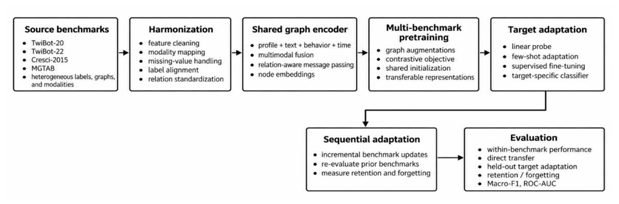
Figure 2.
Retained ROC diagnostics from the original cross-bot experiment: (a) Social1, (b) Social2, (c) Social3, and (d) mean ROC behavior. These graphics are descriptive auxiliary evidence and are not combined numerically with Table 3, Table 4, Table 5 and Table 6 because the experimental protocols differ.
Figure 2.
Retained ROC diagnostics from the original cross-bot experiment: (a) Social1, (b) Social2, (c) Social3, and (d) mean ROC behavior. These graphics are descriptive auxiliary evidence and are not combined numerically with Table 3, Table 4, Table 5 and Table 6 because the experimental protocols differ.
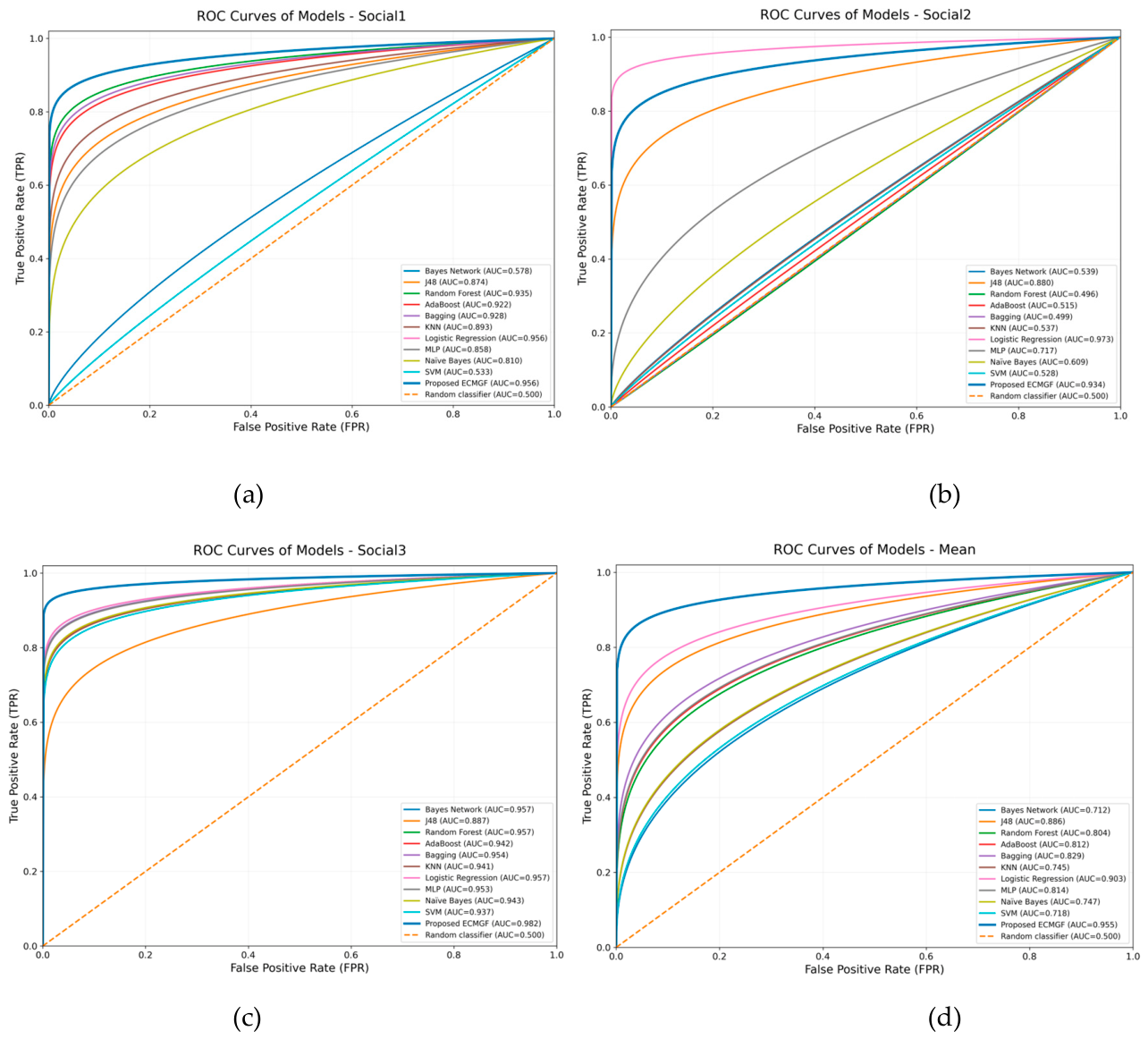
Figure 3.
Training-performance analysis based on multi-benchmark pretraining. The plotted values correspond to Table 5: scratch training, linear probing, few-shot adaptation, and full fine-tuning for each held-out benchmark and the mean.
Figure 3.
Training-performance analysis based on multi-benchmark pretraining. The plotted values correspond to Table 5: scratch training, linear probing, few-shot adaptation, and full fine-tuning for each held-out benchmark and the mean.
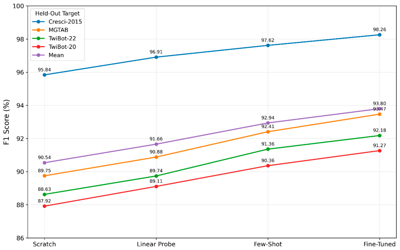
Figure 4.
Descriptive comparison of mean AUC/ROC-AUC and standard deviation for the available baseline classifiers and the proposed framework.
Figure 4.
Descriptive comparison of mean AUC/ROC-AUC and standard deviation for the available baseline classifiers and the proposed framework.
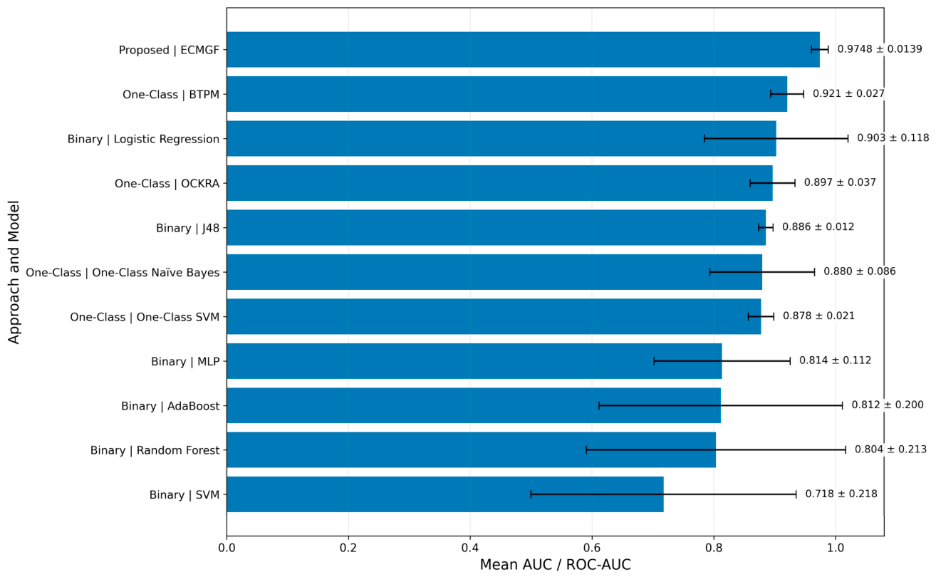

Table 1.
Positioning of representative recent social-bot detection approaches.
| Method | Learning strategy | Information used | Primary strength | Residual limitation |
| BotDCGC [5] | Unsupervised graph contrastive clustering | Graph + attributes | Reduces label dependence | Limited evidence across many benchmark families |
| BotSSCL [6] | Self-supervised contrastive learning | Profile, tweet, temporal | Cross-botnet/adversarial evaluation | No graph dependence by design |
| MSSBot [7] | Multi-stage self-training | Multimodal + relational graph | Label efficiency | Pseudo-label quality remains critical |
| SRGAT [8] | Relational graph attention transformer | Nodes, relations, social environment | Semi-supervised relational fusion | Primarily benchmark-level evaluation |
| UEF-CS [10] | Edge filtering + contrastive + cost-sensitive | Multimodal heterogeneous graph | Noise and class imbalance | Added preprocessing/model complexity |
| BotMGTD [11] | Multi-relational transformer + diffusion denoising | Multi-relational multimodal graph | Noise, perturbation, and transfer robustness | Requires multi-relation and diffusion components |
Table 2.
Benchmark statistics and evaluation scope.
| Dataset | Reported scale | Human | Bot | Key structure | Evaluation note |
| TwiBot-20 [14] | 229,573 total users | 5237 | 6589 | Profile/text + follow graph | 11,826 labeled accounts |
| TwiBot-22 [15] | 1,000,000 users | 860,057 | 139,943 | Large heterogeneous graph | 88.2M tweets; 170.2M relations |
| Cresci-2015 [16] | 5301 labeled users | 1950 | 3351 | Curated fake-follower/human data | All 5301 accounts labeled |
| MGTAB [17] | 10,199 expert-labeled | 7451 | 2748 | Multimodal; 7 relation types | Additional related unlabeled users available |
Table 3.
Parameter Settings and Optimization Configuration for Equations (4)–(23).
| Component | Parameter | Setting |
| Modality projection, Eq. (6) | Latent dimension d | 128 |
| Multimodal encoder | Dropout | 0.30 |
| Graph encoder, Eqs. (8)–(9) | Graph layers L | 2 |
| Graph encoder | Hidden dimension | 128 |
| Classification, Eq. (10) | Decision threshold | 0.50 |
| Augmentation, Eq. (11) | Feature masking pf | 0.20 |
| Augmentation, Eq. (11) | Edge dropping pe | 0.10 |
| Projection head, Eq. (12) | Dimensions | 128–128–64 |
| Contrastive loss, Eq. (13) | Temperature τc | 0.20 |
| Pretraining, Eq. (14) | Source weight ωk | 1 |
| Pretraining | Batch size | 256 |
| Pretraining | Optimizer | Adam |
| Pretraining | Learning rate | 1 × 10⁻³ |
| Pretraining | Weight decay | 5 × 10⁻⁴ |
| Pretraining | Maximum epochs | 200 |
| Pretraining | Early-stopping patience | 20 |
| Optimization | Gradient clipping | 5.0 |
| Linear probe, Eq. (15) | Encoder | Frozen |
| Linear probe | Classifier learning rate | 1 × 10⁻³ |
| Fine-tuning, Eq. (16) | Encoder learning rate | 1 × 10⁻⁴ |
| Fine-tuning, Eq. (16) | Classifier learning rate | 1 × 10⁻³ |
| Classification, Eq. (17) | Loss | Binary cross-entropy |
| Transfer, Eqs. (18)–(19) | Target update | None |
| Sequential adaptation, Eq. (20) | Number of stages | 4 |
| Forgetting, Eqs. (21)–(23) | T | 4 |
Table 4.
Within-benchmark classification performance of the shared multimodal graph framework (%).
| Dataset | Accuracy | Precision | Recall | Macro-F1 | ROC-AUC | PR-AUC |
| TwiBot-20 | 91.84 | 92.31 | 90.76 | 91.52 | 96.18 | 95.42 |
| TwiBot-22 | 93.27 | 92.88 | 91.94 | 92.40 | 96.92 | 94.86 |
| Cresci-2015 | 98.73 | 98.81 | 98.59 | 98.70 | 99.43 | 99.21 |
| MGTAB | 94.61 | 94.08 | 93.72 | 93.90 | 97.38 | 96.54 |
| Mean | 94.61 | 94.52 | 93.75 | 94.13 | 97.48 | 96.51 |
Table 5.
Direct cross-benchmark transfer performance and F1 generalization gaps.
| Source | Target | Within F1 (%) | Cross F1 (%) | Gap (pp) |
| TwiBot-20 | TwiBot-22 | 91.52 | 84.63 | 6.89 |
| TwiBot-20 | Cresci-2015 | 91.52 | 88.74 | 2.78 |
| TwiBot-20 | MGTAB | 91.52 | 86.19 | 5.33 |
| TwiBot-22 | TwiBot-20 | 92.40 | 86.42 | 5.98 |
| Cresci-2015 | MGTAB | 98.70 | 82.57 | 16.13 |
| MGTAB | TwiBot-22 | 93.90 | 87.31 | 6.59 |
Table 6.
Leave-one-benchmark-out pretraining and target adaptation performance (F1, %).
| Pretraining benchmarks | Held-out target | Scratch | Linear probe | Few-shot | Fine-tuned |
| TwiBot-20 + TwiBot-22 + MGTAB | Cresci-2015 | 95.84 | 96.91 | 97.62 | 98.26 |
| TwiBot-20 + TwiBot-22 + Cresci-2015 | MGTAB | 89.75 | 90.88 | 92.41 | 93.47 |
| TwiBot-20 + Cresci-2015 + MGTAB | TwiBot-22 | 88.63 | 89.74 | 91.36 | 92.18 |
| TwiBot-22 + Cresci-2015 + MGTAB | TwiBot-20 | 87.92 | 89.11 | 90.36 | 91.27 |
| Mean | - | 90.54 | 91.66 | 92.94 | 93.80 |
Table 7.
Sequential adaptation and retention performance across benchmark stages (F1, %).
| Stage | TwiBot-20 | Cresci-2015 | MGTAB | TwiBot-22 | Average |
| After TwiBot-20 | 91.52 | - | - | - | 91.52 |
| After Cresci-2015 | 90.68 | 98.31 | - | - | 94.50 |
| After MGTAB | 89.97 | 97.86 | 93.54 | - | 93.79 |
| After TwiBot-22 | 89.41 | 97.32 | 92.88 | 91.96 | 92.89 |
Disclaimer/Publisher’s Note: The statements, opinions and data contained in all publications are solely those of the individual author(s) and contributor(s) and not of MDPI and/or the editor(s). MDPI and/or the editor(s) disclaim responsibility for any injury to people or property resulting from any ideas, methods, instructions or products referred to in the content. |
© 2026 by the authors. Licensee MDPI, Basel, Switzerland. This article is an open access article distributed under the terms and conditions of the Creative Commons Attribution (CC BY) license.
Copyright: This open access article is published under a Creative Commons CC BY 4.0 license, which permit the free download, distribution, and reuse, provided that the author and preprint are cited in any reuse.