
Submitted:
04 October 2026
Posted:
07 October 2026
You are already at the latest version
Abstract
This study examines the relationship between underwriting concentration and financial stability indicators in Egyptian conventional property and liability insurance companies. Using a balanced panel of 17 insurers over 2020–2024 (85 firm-year observations), underwriting concentration is measured using the Herfindahl–Hirschman Index (HHI) based on written premiums across insurance lines. Financial stability is assessed using seven indicators covering profitability (ROA and ROE), liquidity (Current Ratio and Cash Ratio), and solvency/financial structure (D/E, TD/TA, and SER). Separate panel regressions are estimated using Pooled OLS, Fixed Effects, or Random Effects, as determined by specification tests. The HHI coefficient is negative for six of the seven outcomes. Under the conventional unadjusted 5% criterion, HHI is negatively associated with ROE (β = −0.0000219, p = 0.0238), while the associations with the other six indicators are not statistically significant. However, the ROE result does not remain significant under a Bonferroni adjustment for the seven HHI tests (adjusted threshold α = 0.0071). Overall, the findings do not provide robust evidence of a systematic relationship between underwriting concentration and the financial stability indicators examined, although the unadjusted ROE result provides suggestive evidence warranting further investigation.
Keywords:
underwriting concentration
; financial stability
; Herfindahl–Hirschman Index
; property and liability insurance
; panel data
; diversification
1. Introduction
The insurance sector plays an important role in the financial system by providing protection against financial losses, facilitating risk transfer, and supporting economic activity and financial stability. Owing to the nature of their operations, insurance companies are exposed to multiple sources of risk, including underwriting, market, credit, liquidity, operational, and concentration risks. Effective identification, assessment, and management of these risks are therefore important for maintaining insurers’ financial strength and their ability to meet obligations to policyholders (International Association of Insurance Supervisors [IAIS], 2024). Underwriting concentration represents an important dimension of insurers’ risk profiles. Insurance companies may distribute their underwriting activities across multiple lines of business or concentrate a substantial proportion of their written premiums in a limited number of lines. Greater diversification may reduce dependence on adverse developments affecting a particular segment, whereas greater concentration may increase exposure to line-specific shocks. At the same time, specialization may generate benefits through underwriting expertise, operational focus, and more efficient resource allocation. Consequently, the relationship between underwriting concentration and insurers’ financial condition is theoretically ambiguous and requires empirical investigation.
This issue is particularly relevant because an insurer’s financial condition is multidimensional. Underwriting concentration may be associated differently with profitability, liquidity, leverage, and capitalization. Evaluating concentration against a single financial measure may therefore provide only a partial view of its relationship with insurer financial stability. A multidimensional approach can provide a broader assessment by examining whether the association with underwriting concentration varies across different aspects of financial condition.
Against this background, the present study examines the relationship between underwriting concentration and financial stability indicators in Egyptian conventional property and liability insurance companies. Underwriting concentration is measured using the Herfindahl–Hirschman Index (HHI), calculated from the distribution of written premiums across insurance lines. Financial stability is assessed using seven indicators covering three dimensions: profitability, represented by return on assets (ROA) and return on equity (ROE); liquidity, represented by the Current Ratio (CR) and Cash Ratio (CashR); and solvency and financial structure, represented by the Debt-to-Equity Ratio (D/E), Total Debt-to-Total Assets Ratio (TD/TA), and Shareholders’ Equity-to-Total Assets Ratio (SER).
The empirical analysis is based on a balanced panel of 17 Egyptian conventional property and liability insurance companies over the period 2020–2024, comprising 85 firm-year observations. The study controls for firm size, premium growth, firm age, loss ratio, expense ratio, reliance on reinsurance, and investment yield. Alternative panel-data specifications are considered to account for unobserved firm-level heterogeneity and to identify the appropriate specification for each financial indicator.
The study contributes to the insurance literature in three respects. First, it focuses specifically on within-firm underwriting concentration across insurance lines, distinguishing this concept from market concentration among competing insurers. Second, it evaluates the relationship between underwriting concentration and financial condition using multiple indicators representing profitability, liquidity, and solvency/financial structure rather than relying on a single performance measure. Third, it provides empirical evidence from the Egyptian insurance market, contributing to the comparatively limited evidence on underwriting concentration in emerging-market insurance settings.
The remainder of the paper is organized as follows. Section 2 reviews the relevant literature and develops the study hypothesis. Section 3 describes the data, variables, and econometric methodology. Section 4 presents the empirical results. Section 5 discusses the findings and their implications. Section 6 concludes the study, outlines its limitations, and identifies directions for future research.
2. Literature Review and Hypothesis Development
2.1. Underwriting Concentration and Diversification in Insurance
Underwriting concentration reflects the extent to which an insurer’s underwriting portfolio is concentrated in a limited number of lines of business. Its potential financial consequences can be understood from two competing perspectives. From a diversification perspective, spreading underwriting activity across multiple lines may reduce dependence on losses arising from any single business segment and may provide risk-pooling benefits when underwriting outcomes across lines are imperfectly correlated. Conversely, the strategic-focus perspective suggests that specialization may generate advantages through greater underwriting expertise, lower organizational complexity, more effective monitoring, and more efficient allocation of managerial resources.
These competing mechanisms are particularly relevant to property and liability insurers, whose lines of business may differ substantially in loss distributions, underwriting cycles, capital requirements, and exposure to economic and catastrophic shocks. Consequently, greater diversification does not necessarily produce superior financial outcomes, nor does greater concentration necessarily imply weaker performance. The net relationship depends on whether the benefits of risk spreading outweigh the potential costs associated with organizational complexity, agency problems, and inefficient resource allocation.
The benefits of diversification are also not necessarily uniform across different risk structures. Degen et al. (2010) demonstrate that the effects of risk aggregation depend on the characteristics and dependence structure of the underlying risks and that, under certain conditions, aggregation may even produce negative diversification benefits. This evidence reinforces the theoretical ambiguity surrounding underwriting concentration, as the benefits of risk spreading cannot be assumed to arise uniformly across different insurance portfolios.
The insurance literature provides evidence supporting both perspectives. Liebenberg and Sommer (2008) examined U.S. property–liability insurers during 1995–2004 and found that undiversified insurers consistently outperformed diversified insurers. They reported a diversification penalty in accounting performance, including both return on assets and return on equity, as well as a diversification discount based on a market-value measure. Their findings therefore provide support for the strategic-focus hypothesis, under which specialization may generate performance advantages relative to broader diversification.
However, the diversification–performance relationship does not appear to be universally linear. Elango et al. (2008), using U.S. property–liability insurance data for 1994–2002, found a complex and nonlinear relationship between product diversification and firm performance. They further showed that the performance implications of product diversification were contingent on insurers’ degree of geographic diversification. These findings suggest that the financial consequences of diversification may depend on the extent and form of diversification rather than following a uniform positive or negative pattern.
The decision to diversify may itself reflect several organizational and market considerations. Berry-Stölzle et al. (2012) examined the determinants of line-of-business diversification among property–liability insurers and found that diversification was not driven solely by risk-pooling considerations. Instead, their evidence indicates that internal capital-market benefits and barriers to business growth, including market size and concentration, help explain insurers’ diversification decisions. They also distinguish between related and unrelated diversification, reinforcing the view that diversification should not be treated as a homogeneous corporate strategy.
The effects of diversification may also extend beyond profitability and may interact with other dimensions of insurer risk. Che and Liebenberg (2017), examining U.S. property–liability insurers, found that greater line-of-business diversification was associated with greater asset risk-taking, consistent with the coordinated risk-management hypothesis. This finding suggests that changes in underwriting diversification may be accompanied by adjustments in other components of an insurer’s overall risk profile.
More recent evidence further indicates that the consequences of diversification may differ across institutional and organizational settings. Chen (2026), examining Chinese non-life insurers, found that the effects of product and geographic diversification on underwriting and asset risks vary according to ownership structure and risk distribution. This evidence further supports the view that the relationship between concentration, diversification, and insurer financial outcomes may be heterogeneous across firms and markets.
Taken together, these studies demonstrate that underwriting specialization and diversification involve competing benefits and costs. Greater concentration may facilitate specialization and operational focus, while diversification may provide risk-spreading benefits. The resulting financial effect is therefore an empirical question that may vary according to the financial outcome examined and the characteristics of the insurer and its operating environment.
2.2. Concentration and Insurer Financial Stability
The implications of concentration extend beyond conventional profitability measures. An insurer’s underwriting structure may also be related to liquidity, leverage, capitalization, and its broader ability to absorb adverse financial developments. A highly concentrated underwriting portfolio may increase exposure to shocks affecting dominant lines of business, whereas diversification may reduce dependence on individual segments. At the same time, diversification may introduce additional organizational and monitoring costs, meaning that its contribution to financial stability cannot be assumed to be uniformly beneficial.
Evidence from the broader market-concentration literature provides a complementary perspective on the relationship between concentration and insurer financial stability. Using a large international sample of property–liability insurers, Altuntas and Rauch (2017) found that higher market concentration was associated with lower financial stability, providing evidence consistent with the concentration-fragility view. Although their analysis concerns concentration at the insurance-market level rather than underwriting concentration within individual insurers, their findings demonstrate the broader relevance of concentration to insurer financial stability.
Related evidence is provided by Shim (2017), who investigated the relationship between market concentration and financial stability in the U.S. property–liability insurance industry over 1992–2010. Using instrumental-variable estimation to address potential endogeneity, the study found that higher market concentration was associated with lower insurer financial stability, consistent with the concentration-fragility view. The study also identified firm characteristics such as size, underwriting leverage, organizational form, product and geographic diversification, catastrophe exposure, and macroeconomic conditions as relevant determinants of insurer financial stability.
A conceptual distinction is necessary, however. Shim (2017) examines market concentration, which refers to the distribution of market shares among competing insurers. The present study examines within-firm underwriting concentration, which concerns the distribution of an individual insurer’s written premiums across insurance lines. The two concepts are therefore not interchangeable. Nevertheless, the financial-stability literature demonstrates that concentration and diversification can interact with insurer risk and financial resilience, providing a broader theoretical foundation for investigating concentration within underwriting portfolios.
The distinction is particularly important in the present study because financial stability is not represented by a single outcome. Instead, the analysis considers profitability through ROA and ROE, liquidity through the Current Ratio and Cash Ratio, and solvency and financial structure through D/E, TD/TA, and SER. This multidimensional specification corresponds to the empirical design of the study, which estimates separate panel models for each of the seven indicators.
2.3. Research Gap
The existing literature provides substantial evidence that diversification and concentration may influence insurer performance and risk. However, several limitations leave scope for further investigation.
First, much of the established empirical evidence online-of-business diversification is based on the U.S. property–liability insurance market. Liebenberg and Sommer (2008) and Elango et al. (2008), for example, provide important evidence concerning U.S. insurers, but their findings do not imply that the same relationships necessarily apply in insurance markets characterized by different regulatory, competitive, and institutional conditions.
Second, previous studies demonstrate that diversification is multidimensional and that its consequences may depend on how diversification is structured. Berry-Stölzle et al. (2012), for example, distinguish between related and unrelated diversification and show that insurers’ diversification decisions are associated with factors beyond risk pooling alone. This suggests that examining the actual concentration of underwriting activity across insurance lines may provide additional information beyond simply classifying insurers as diversified or specialized.
Third, although prior research has examined insurer profitability, diversification, risk-taking, and financial stability, empirical evidence directly relating within-firm underwriting concentration across lines of business to multiple dimensions of insurers’ financial condition remains comparatively limited, particularly in emerging insurance markets. The distinction between market-level concentration and firm-level underwriting concentration is especially important in this context.
The present study addresses this gap by examining 17 conventional Egyptian property and liability insurers over 2020–2024, producing a balanced panel of 85 firm-year observations. Underwriting concentration is measured continuously using the Herfindahl–Hirschman Index based on the distribution of written premiums across insurance lines.
Rather than relying on a single measure of insurer performance, the study examines seven indicators representing profitability, liquidity, and solvency/financial structure. This approach allows the association between underwriting concentration and financial condition to differ across financial dimensions rather than imposing the assumption that concentration has a uniform effect on all aspects of insurer performance.
2.4. Hypothesis Development
The preceding literature provides competing theoretical predictions concerning underwriting concentration.
Under the strategic-focus perspective, greater underwriting concentration may improve financial performance by allowing insurers to develop specialized underwriting expertise, reduce organizational complexity, improve monitoring, and concentrate managerial resources on business lines in which they possess comparative advantages. The empirical findings of Liebenberg and Sommer (2008), who report superior performance among less-diversified property–liability insurers, are consistent with this argument.
Under the diversification perspective, however, spreading underwriting activity across multiple lines may reduce exposure to adverse developments affecting a particular segment and provide risk-pooling benefits. At the same time, the nonlinear findings reported by Elango et al. (2008) and the evidence on the heterogeneous determinants of diversification reported by Berry-Stölzle et al. (2012) indicate that the financial consequences of diversification are unlikely to be uniform across insurers or financial outcomes.
Accordingly, the existing theoretical and empirical literature does not provide sufficiently unambiguous grounds for imposing a directional prediction for all seven financial indicators. The present study therefore formulates a non-directional hypothesis:
H1: Underwriting concentration is significantly associated with the financial stability indicators of Egyptian conventional property and liability insurance companies.
This hypothesis is evaluated separately across the seven financial indicators—ROA, ROE, Current Ratio, Cash Ratio, D/E, TD/TA, and SER—recognizing that the relationship between underwriting concentration and financial condition may differ across profitability, liquidity, and solvency dimensions.
3. Materials and Methods
3.1. Research Design and Sample
This study adopts a quantitative longitudinal research design to examine the relationship between underwriting concentration and financial stability indicators in Egyptian conventional property and liability insurance companies. The empirical analysis is based on balanced panel data covering the period 2020–2024.
The Egyptian property and liability insurance market comprised 23 companies within the scope of the study, consisting of 17 conventional insurance companies and six takaful insurance companies. The study focuses exclusively on the 17 companies operating under the conventional insurance model. Accordingly, the six property and liability takaful insurers were excluded to maintain comparability in financial and underwriting data and to obtain a more homogeneous sample in terms of insurance business model.
The final sample therefore comprises 17 conventional property and liability insurance companies for which the data required to construct the underwriting concentration measure, financial stability indicators, and control variables were available throughout the study period. This results in a balanced panel of 85 firm-year observations (17 companies × 5 years).
The analysis is restricted to companies with complete and comparable observations over the five-year period. Accordingly, the empirical findings are interpreted within the sample, period, variables, and econometric specifications employed. The estimated relationships should therefore be interpreted as associations rather than as evidence of causal effects.
3.2. Data Sources
The study relies on secondary financial and underwriting data obtained from the annual statistical reports published by the Egyptian Financial Regulatory Authority (FRA), together with the published financial statements and annual reports of the insurance companies included in the sample.
Underwriting data consist of written premiums by line of business and are used to calculate the Herfindahl–Hirschman Index (HHI) for each insurer-year observation. Financial statement data are used to construct the seven financial stability indicators and the firm-specific control variables. A consistent measurement procedure is applied across insurers and years to enhance comparability within the balanced panel dataset.
3.3. Measurement of Underwriting Concentration
Underwriting concentration is the main explanatory variable and is measured using the Herfindahl–Hirschman Index (HHI). The index is calculated separately for each insurer and each year based on the distribution of written premiums across insurance lines.
The underwriting share of insurance line jfor company iin year tis calculated as:
where Sijtrepresents the share of insurance line jin the total written premiums of company iin year t, WPijtrepresents written premiums for insurance line j, and nrepresents the number of insurance lines.
The HHI is then calculated as:
When underwriting shares are expressed as percentages, the HHI ranges from approximately 0 to 10,000. Higher HHI values indicate greater underwriting concentration, whereas lower values indicate greater diversification across insurance lines.
The calculation covers the relevant property and liability insurance lines reported in the available underwriting data, including Fire, Marine Cargo, Inland Transport, Marine Hull, Aviation, Motor, Engineering, Oil and Gas, Accident, and Medical Insurance. The same procedure is applied consistently across insurers and years.
For descriptive purposes, HHI values below 1,500 are treated as relatively low concentration, values between 1,500 and 2,500 as moderate concentration, and values above 2,500 as relatively high concentration. These classifications are used only for descriptive interpretation; HHI enters the econometric models as a continuous variable.
3.4. Financial Stability Indicators
Financial stability is assessed across three dimensions: profitability, liquidity, and solvency/financial structure. Seven dependent variables are employed.
Profitability is represented by Return on Assets (ROA) and Return on Equity (ROE). Liquidity is represented by the Current Ratio (CR) and Cash Ratio (CashR). Solvency and financial structure are represented by the Debt-to-Equity Ratio (D/E), Total Debt-to-Total Assets Ratio (TD/TA), and Shareholders’ Equity-to-Total Assets Ratio (SER).
The indicators are calculated as follows:
and
3.5. Control Variables
Seven firm-specific control variables are included to account for differences in the financial and operational characteristics of the insurers. SIZE is measured as the natural logarithm of total assets. GROWTH represents the annual growth rate of gross written premiums. AGE represents the number of years between the company’s establishment and the year of observation. LOSS measures claims relative to earned premiums. EXPR measures general and administrative expenses relative to earned premiums. RINS measures the proportion of gross written premiums ceded to reinsurers. INV measures the return generated from invested assets.
These variables are calculated consistently for each company-year over the study period.
3.6. Econometric Model Specification
Separate panel-data regression models are estimated for each of the seven financial stability indicators. The general empirical specification is:
where FSitrepresents one of the seven financial stability indicators for insurer iin year t; HHIitrepresents underwriting concentration; SIZE, GROWTH, AGE, LOSS, EXPR, RINS, and INV represent the control variables; αis the intercept; and εitis the error term.
Seven models are estimated separately, with ROA, ROE, CR, CashR, D/E, TD/TA, and SER serving in turn as the dependent variable.
3.7. Panel-Data Model Selection
Three alternative panel-data specifications are considered: Pooled Ordinary Least Squares (Pooled OLS), Fixed Effects (FE), and Random Effects (RE). Model selection is conducted separately for each dependent variable using a sequence of specification tests.
The Redundant Fixed Effects Test is used to assess whether cross-sectional fixed effects are jointly significant relative to the pooled specification. The Breusch–Pagan Lagrange Multiplier (LM) test evaluates whether the random-effects specification provides an improvement over Pooled OLS. When panel effects are supported, the Hausman specification test is used to assess the appropriateness of the Random Effects estimator relative to the Fixed Effects estimator. This model-selection strategy follows standard panel-data econometric principles (Baltagi, 2021; Wooldridge, 2010).
Because the appropriate specification may differ across financial outcomes, the model-selection tests are conducted separately for each of the seven dependent variables. The final specification for each financial stability indicator is determined by considering the results of these tests jointly rather than imposing a common estimator across all seven models.
4. Results
4.1. Descriptive Statistics
Table 1 presents the descriptive statistics for the study variables across the 85 firm-year observations.
The mean HHI is 3,906, with a standard deviation of 2,091.20, indicating substantial variation in underwriting concentration across insurer-year observations. The mean ROA and ROE are 0.06 and 0.16, respectively. The mean Current Ratio and Cash Ratio are 3.90 and 0.19, while the mean D/E, TD/TA, and SER are 2.20, 0.60, and 0.38, respectively.
The Jarque–Bera results indicate that HHI, SER, and INV do not significantly depart from normality at the 5% level, whereas the remaining variables exhibit statistically significant departures from normality. These descriptive results characterize the distribution of the variables but do not, by themselves, determine the appropriate panel-data specification or statistical inference.
To provide a clearer view of cross-sectional differences in underwriting concentration, Figure 1 presents the average HHI for each insurer over the 2020–2024 study period.
Figure 1 reveals substantial cross-sectional variation in underwriting concentration across the sampled insurers. Misr Insurance records the lowest average HHI over the study period, remaining below the descriptive threshold of 1,500, whereas several insurers exhibit substantially higher average concentration levels. Tharwa Insurance records the highest average HHI, followed by AIG Insurance and AXA Insurance. The observed variation indicates considerable heterogeneity in the degree of underwriting concentration across insurers and supports the treatment of HHI as a continuous firm-level variable in the subsequent panel-data analysis.
4.2. Correlation Analysis
Table 2 presents the correlation matrix.
Table 2 presents the pairwise correlation matrix for the variables included in the analysis. The correlations between HHI and the seven financial stability indicators are generally weak, providing no preliminary indication of a strong linear association between underwriting concentration and any individual financial outcome.
Among the explanatory variables, the relatively high correlation between GROWTH and RINS (0.775) warrants caution when interpreting their individual regression coefficients. Correlations observed among the dependent variables, including ROA and ROE (0.789) and D/E and TD/TA (0.785), do not directly generate multicollinearity within the estimated regressions because these financial indicators enter separate models as dependent variables.
4.3. Panel-Data Model Selection Results
4.3.1. Breusch–Pagan LM Test
Table 3 reports the Breusch–Pagan Lagrange Multiplier (LM) test results. The null hypothesis of no significant panel-level random effect is rejected for ROA, Current Ratio, Cash Ratio, D/E, TD/TA, and SER. For these six outcomes, the results provide evidence in favor of a panel specification relative to Pooled OLS. For ROE, however, the LM test is statistically insignificant (p = 0.7887), providing no evidence that the Random Effects specification improves upon Pooled OLS.
4.3.2. Redundant Fixed Effects Test
Table 4 presents the Redundant Fixed Effects test results. The null hypothesis that the cross-sectional fixed effects are redundant is rejected for ROA, Current Ratio, Cash Ratio, D/E, TD/TA, and SER, supporting the Fixed Effects specification over Pooled OLS for these outcomes. For ROE, neither the cross-section F statistic nor the cross-section Chi-square statistic is statistically significant, indicating that Pooled OLS remains adequate relative to the Fixed Effects specification.
4.3.3. Hausman Test
Table 5 reports the Hausman specification test results. The null hypothesis underlying the Random Effects specification is rejected for ROA (p = 0.0437), Current Ratio (p = 0.0451), Cash Ratio (p < 0.001), and D/E (p = 0.0041), supporting the Fixed Effects estimator for these outcomes. In contrast, the Hausman test does not reject the Random Effects specification for TD/TA (p = 0.4036) or SER (p = 0.1472). Although the Hausman statistic for ROE is statistically insignificant (p = 0.6982), the preceding LM and Redundant Fixed Effects tests provide no evidence that either Random Effects or Fixed Effects is preferable to Pooled OLS. Accordingly, Pooled OLS is retained for ROE.
Considering the specification tests jointly, the final models are therefore: Fixed Effects for ROA, Current Ratio, Cash Ratio, and D/E; Random Effects for TD/TA and SER; and Pooled OLS for ROE.
4.4. Regression Results
Table 6 reports the estimated relationship between underwriting concentration and each of the seven financial stability indicators using the model specification selected for the respective outcome. The HHI coefficient is negative for six of the seven financial stability indicators. Under the conventional unadjusted 5% significance criterion, a statistically significant relationship is identified only for ROE (β = −0.0000219, p = 0.0238), indicating a negative association between underwriting concentration and ROE within the estimated model.
No statistically significant relationship is identified for ROA (p = 0.9150), Current Ratio (p = 0.6687), Cash Ratio (p = 0.8565), D/E (p = 0.8093), TD/TA (p = 0.4412), or SER (p = 0.7440). TD/TA is the only indicator with a positive HHI coefficient; however, because this coefficient is statistically insignificant, its direction should not be interpreted as evidence of an established positive relationship. Because the HHI coefficient is tested across seven financial outcomes, the results are also considered in light of multiple testing. A Bonferroni adjustment for seven tests yields a family-wise 5% significance threshold of approximately 0.0071 (0.05/7). The ROE p-value of 0.0238 does not meet this adjusted threshold. Therefore, although the ROE association is statistically significant under the conventional unadjusted criterion, it does not remain significant after the Bonferroni adjustment.
The results provide suggestive evidence of a negative association between underwriting concentration and ROE under the unadjusted criterion, but they do not provide robust evidence of a systematic relationship between underwriting concentration and the seven financial stability indicators after accounting for multiple testing.
5. Discussion
This study examines the relationship between underwriting concentration and multiple dimensions of financial stability in Egyptian conventional property and liability insurance companies. The results indicate that the relationship is not uniform across the seven financial indicators examined. The HHI coefficient is negative for six of the seven outcomes, but under the conventional unadjusted 5% significance level, the relationship is statistically significant only for ROE (β = −0.0000219, p = 0.0238). No statistically significant association is identified for ROA, the Current Ratio, the Cash Ratio, D/E, TD/TA, or SER.
The negative coefficient for ROE suggests that, before adjustment for multiple testing, greater underwriting concentration is associated with lower returns to shareholders’ equity. One possible interpretation is that greater dependence on a limited number of insurance lines may increase exposure to adverse developments affecting dominant segments and reduce the potential risk-spreading benefits associated with a more diversified underwriting portfolio. However, the estimated relationship is associative rather than causal, and the result should not be interpreted as demonstrating that greater underwriting concentration necessarily causes lower ROE.
The ROE finding differs from the evidence reported by Liebenberg and Sommer (2008), who found that less-diversified U.S. property–liability insurers outperformed more diversified insurers and documented a diversification penalty in accounting and market-based performance measures. This difference illustrates that the financial consequences of concentration and diversification may depend on the market, period, institutional environment, and specific performance measure considered.
The findings are also consistent with the broader view that the diversification–performance relationship is heterogeneous rather than uniformly positive or negative. Elango et al. (2008) found a complex and nonlinear relationship between product diversification and insurer performance and showed that its implications depend partly on geographic diversification. Berry-Stölzle et al. (2012) further demonstrated that insurers’ diversification decisions reflect considerations beyond risk pooling, including internal capital-market benefits and barriers to business growth.
The absence of a statistically significant association between HHI and ROA is particularly relevant because ROA and ROE represent different dimensions of profitability. Whereas ROA reflects earnings relative to the insurer’s asset base, ROE measures earnings relative to shareholders’ equity and is therefore more sensitive to capitalization and financial structure. Consequently, the unadjusted ROE result should not be generalized as evidence that underwriting concentration is systematically associated with overall insurer profitability.
The liquidity results provide no statistically significant evidence that underwriting concentration is associated with either the Current Ratio or the Cash Ratio. Within the sample and study period examined, therefore, greater concentration across underwriting lines is not shown to correspond systematically to insurers’ short-term liquidity positions.
Similarly, the solvency and financial-structure indicators do not show statistically significant relationships with underwriting concentration. Although the HHI coefficients for D/E and SER are negative and the coefficient for TD/TA is positive, none is statistically significant. A concentrated underwriting portfolio therefore does not necessarily translate directly into greater leverage, a higher debt-to-assets ratio, or a lower equity ratio within the same financial year.
More broadly, the findings are consistent with the view that the consequences of concentration and diversification can differ according to the type of risk, firm characteristics, and financial outcome considered. Degen et al. (2010) show that diversification benefits depend on the characteristics and dependence structure of the underlying risks. Previous insurance research also indicates that business diversification may interact with other components of insurer risk-taking (Che & Liebenberg, 2017), while more recent evidence suggests that diversification effects may vary according to ownership structure and the form of diversification adopted (Chen, 2026).
Evidence from the market-concentration literature provides an additional but conceptually distinct perspective. Altuntas and Rauch (2017) and Shim (2017) report evidence linking greater market concentration to lower insurer financial stability. However, market concentration refers to the distribution of business among competing insurers, whereas the HHI employed in the present study measures the concentration of underwriting activity across lines of business within an individual insurer. Accordingly, these findings provide useful contextual evidence but should not be interpreted as directly equivalent to the within-firm relationship examined in this study.
5.1. Multiple-Testing Considerations
An important consideration in interpreting the results is that the HHI coefficient is evaluated separately across seven financial outcomes. Conducting multiple statistical tests increases the probability of obtaining at least one statistically significant result by chance when conventional significance thresholds are applied independently to each regression.
Under the conventional unadjusted 5% criterion, the ROE coefficient is statistically significant at p = 0.0238. However, applying a Bonferroni adjustment for the seven HHI tests results in a family-wise significance threshold of approximately 0.0071 (0.05/7). Because 0.0238 exceeds this adjusted threshold, the ROE association does not remain statistically significant under the Bonferroni correction.
Accordingly, the negative association between underwriting concentration and ROE should be interpreted as suggestive evidence under the conventional unadjusted criterion rather than as a robust confirmatory finding. When the seven HHI tests are considered jointly, the results do not provide statistically robust evidence that underwriting concentration is systematically associated with the broader set of financial stability indicators examined in this study.
This interpretation does not establish that underwriting concentration has no financial relevance. Rather, it indicates that the available evidence from the present sample, period, and econometric specifications is insufficient to establish a robust systematic relationship after accounting for multiple testing. The unadjusted ROE result may therefore provide a basis for further investigation using larger samples, longer observation periods, and alternative empirical specifications.
5.2. Practical and Research Implications
The results reinforce the importance of assessing underwriting concentration within a multidimensional risk-management framework. HHI can provide useful information about the distribution of underwriting activity across business lines, but it should not be interpreted as a stand-alone indicator of financial vulnerability. Instead, concentration measures may be evaluated alongside profitability, liquidity, capitalization, leverage, loss experience, reinsurance dependence, and investment performance.
For insurers, periodic monitoring of underwriting concentration may support portfolio-management and enterprise risk-management processes by identifying excessive dependence on particular lines of business. However, the absence of robust statistical significance across the seven financial indicators suggests that concentration levels should be interpreted in conjunction with the insurer’s broader risk profile rather than automatically classified as beneficial or detrimental.
For regulators and supervisors, the distinction between market concentration and within-firm underwriting concentration is also important. Market-level concentration measures such as those examined by Altuntas and Rauch (2017) and Shim (2017) address competitive structure, whereas firm-level HHI across insurance lines captures the composition of an individual insurer’s underwriting portfolio. These measures may therefore provide different but complementary information within risk-based supervisory and early-warning frameworks.
6. Conclusions
This study examined the relationship between underwriting concentration and financial stability in Egyptian conventional property and liability insurance companies using a balanced panel of 17 insurers over the period 2020–2024, comprising 85 firm-year observations. Underwriting concentration was measured using the Herfindahl–Hirschman Index (HHI) based on the distribution of written premiums across insurance lines, while financial stability was assessed using seven indicators covering profitability, liquidity, and solvency/financial structure.
The empirical results indicate that the relationship between underwriting concentration and financial stability is not uniform across the indicators examined. The HHI coefficient is negative for six of the seven financial outcomes. Under the conventional unadjusted 5% significance criterion, underwriting concentration is negatively associated with ROE (β = −0.0000219, p = 0.0238), whereas no statistically significant association is identified for ROA, the Current Ratio, the Cash Ratio, D/E, TD/TA, or SER.
However, because the HHI coefficient is evaluated across seven financial outcomes, the individual significance tests should also be considered within a multiple-testing framework. Applying a Bonferroni adjustment produces a family-wise 5% significance threshold of approximately 0.0071. The ROE result does not satisfy this adjusted threshold. Accordingly, the negative association between underwriting concentration and ROE should be interpreted as suggestive under the conventional unadjusted criterion rather than as a robust confirmatory finding. Taken jointly, the seven tests do not provide statistically robust evidence of a systematic relationship between underwriting concentration and the financial stability indicators examined.
The findings therefore emphasize the importance of evaluating underwriting concentration within a multidimensional framework. HHI provides information about the distribution of underwriting activity across insurance lines, but concentration alone should not be interpreted as sufficient evidence of financial strength or vulnerability. Insurers and regulators may instead consider underwriting concentration alongside profitability, liquidity, capitalization, leverage, loss experience, reinsurance arrangements, investment performance, and other firm-specific characteristics.
From a managerial perspective, periodic monitoring of HHI may assist insurers in identifying excessive dependence on particular lines of business and may complement broader portfolio-management and enterprise risk-management processes. However, concentration levels should be interpreted in the context of the insurer’s overall risk profile rather than being treated as inherently beneficial or detrimental.
From a regulatory perspective, within-firm underwriting concentration may provide information that complements, rather than substitutes for, conventional financial and risk-based supervisory indicators. It is also important to distinguish underwriting concentration across business lines from market concentration among competing insurers, as the two concepts capture different dimensions of concentration.
The study is subject to several limitations. First, the analysis is based on 17 conventional Egyptian property and liability insurers over a five-year period, which limits the extent to which the findings can be generalized beyond the sample and study period. Second, takaful insurers are excluded to maintain comparability in the business model and financial and underwriting data; consequently, the findings should not be generalized to the takaful segment. Third, underwriting concentration is measured using written-premium shares across insurance lines, and alternative measures of portfolio concentration may capture different dimensions of underwriting structure. Fourth, the observational panel-data design identifies statistical associations rather than causal effects and may remain subject to omitted-variable and endogeneity concerns. Finally, the relatively short observation period and the evaluation of multiple financial outcomes limit the strength of statistical inference.
Future research could extend the analysis by using longer observation periods, larger samples, and cross-country insurance data. Further studies could also examine individual insurance lines, distinguish between related and unrelated diversification, investigate nonlinear relationships and concentration thresholds, and evaluate lagged effects of underwriting concentration. Alternative empirical strategies addressing potential endogeneity could provide stronger evidence regarding causal relationships. Future research may also investigate whether the relationship between underwriting concentration and financial outcomes varies according to insurer size, capitalization, ownership structure, reinsurance dependence, or business model.
The findings suggest that the relationship between underwriting concentration and insurer financial condition is more nuanced than a simple concentration-versus-diversification distinction. The unadjusted ROE result warrants further investigation, but the evidence from the present sample does not establish a robust systematic relationship between underwriting concentration and the broader set of financial stability indicators after accounting for multiple testing.
Author Contributions
Conceptualization, S.M.G.; methodology, S.M.G.; software, S.M.G.; validation, S.M.G.; formal analysis, S.M.G.; investigation, S.M.G.; resources, S.M.G.; data curation, S.M.G.; writing—original draft preparation, S.M.G.; writing—review and editing, S.M.G.; visualization, S.M.G.; project administration, S.M.G. The author has read and agreed to the published version of the manuscript.
Funding
This research received no external funding.
Institutional Review Board Statement
Not applicable. This study did not involve humans or animals and was based exclusively on secondary financial and underwriting data.
Informed Consent Statement
Not applicable. This study did not involve human participants.
Data Availability Statement
The data used in this study were compiled from publicly available annual statistical reports of the Egyptian Financial Regulatory Authority (FRA) and published financial statements and annual reports of the insurance companies included in the sample. The processed data supporting the findings of this study are available from the corresponding author upon reasonable request.
Acknowledgments
During the preparation of this manuscript, the author used ChatGPT (OpenAI) for language editing, structural organization, and improvement of clarity and presentation. The author reviewed and edited the output and takes full responsibility for the content of this publication.
Conflicts of Interest
The author declare no conflicts of interest.
Abbreviations
The following abbreviations are used in this manuscript:
| AGE | Firm Age |
| CR | Current Ratio |
| CashR | Cash Ratio |
| D/E | Debt-to-Equity Ratio |
| EXPR | Expense Ratio |
| FE | Fixed Effects |
| FRA | Financial Regulatory Authority |
| GROWTH | Premium Growth |
| GWP | Gross Written Premiums |
| HHI | Herfindahl–Hirschman Index |
| INV | Investment Yield |
| LM | Lagrange Multiplier |
| LOSS | Loss Ratio |
| OLS | Ordinary Least Squares |
| RE | Random Effects |
| RINS | Reliance on Reinsurance |
| ROA | Return on Assets |
| ROE | Return on Equity |
| SER | Shareholders’ Equity-to-Total Assets Ratio |
| SIZE | Firm Size |
| TD/TA | Total Debt-to-Total Assets Ratio |
Appendix A
Calculated Financial Stability and Control Variables

Table A1.
Calculated Values of Financial Stability Indicators and Control Variables for the Sampled Insurance Companies, 2020–2024.
Table A1.
Calculated Values of Financial Stability Indicators and Control Variables for the Sampled Insurance Companies, 2020–2024.
| Indicator | Year | Mada Insurance | Watania Insurance | Tharwa Insurance | AXA Insurance | Iskan Insurance | Arope Property Insurance | Bupa Egypt | Allianz Insurance - Egypt | Royal Insurance | Chubb Insurance | Egyptian Cooperative Insurance Society | GIG Insurance | AIG Insurance | Delta Insurance | Al Mohandes Insurance | Suez Canal Insurance | Misr Insurance |
| Return on Assets (ROA) | 20/19 | 0.0 | 0.0 | 0.01 | 0.04 | 0.10 | 0.09 | 0.02 | 0.08 | 0.07 | 0.03 | 0.01 | 0.09 | 0.05 | 0.11 | 0.11 | 0.03 | 0.07 |
| 21/20 | 0.01 | 0.05 | 0.02 | -0.08 | 0.08 | 0.08 | 0.04 | 0.08 | 0.08 | 0.02 | 0.03 | 0.09 | 0.07 | 0.12 | 0.08 | 0.02 | 0.06 | |
| 22/21 | 0.06 | 0.00 | 0.03 | 0.03 | 0.05 | 0.08 | 0.02 | 0.07 | 0.09 | 0.03 | 0.02 | 0.07 | 0.05 | 0.09 | 0.07 | 0.03 | 0.06 | |
| 23/22 | 0.05 | 0.05 | 0.04 | 0.00 | 0.06 | 0.08 | -0.06 | 0.10 | 0.09 | 0.02 | 0.02 | 0.09 | 0.03 | 0.10 | 0.08 | 0.03 | 0.05 | |
| 24/23 | 0.07 | 0.10 | 0.09 | 0.06 | 0.07 | 0.10 | 0.02 | 0.11 | 0.12 | 0.02 | 0.05 | 0.11 | 0.08 | 0.14 | 0.11 | 0.06 | 0.06 | |
| Return on Equity (ROE) | 20/19 | 0.0 | 0.0 | 0.02 | 0.27 | 0.26 | 0.16 | 0.05 | 0.28 | 0.34 | 0.04 | 0.04 | 0.24 | 0.14 | 0.23 | 0.32 | 0.16 | 0.16 |
| 21/20 | 0.02 | 0.06 | 0.05 | -0.9 | 0.20 | 0.15 | 0.11 | 0.25 | 0.31 | 0.03 | 0.08 | 0.24 | 0.16 | 0.24 | 0.22 | 0.13 | 0.12 | |
| 22/21 | 0.04 | 0.01 | 0.11 | 0.27 | 0.15 | 0.14 | 0.06 | 0.30 | 0.32 | 0.05 | 0.06 | 0.22 | 0.10 | 0.19 | 0.20 | 0.15 | 0.12 | |
| 23/22 | 0.16 | 0.10 | 0.11 | 0.03 | 0.21 | 0.14 | -0.2 | 0.24 | 0.29 | 0.03 | 0.06 | 0.30 | 0.05 | 0.25 | 0.22 | 0.18 | 0.08 | |
| 24/23 | 0.18 | 0.40 | 0.71 | 0.29 | 0.23 | 0.18 | 0.05 | 0.61 | 0.38 | 0.03 | 0.15 | 0.42 | 0.13 | 0.34 | 0.30 | 0.29 | 0.09 | |
| Current Ratio (CR) | 20/19 | 0.0 | 0.0 | 8.76 | 2.43 | 3.69 | 6.06 | 1.94 | 3.02 | 3.85 | 2.94 | 2.49 | 2.44 | 2.10 | 4.53 | 2.77 | 1.87 | 6.14 |
| 21/20 | 2.02 | 10.3 | 13.4 | 5.22 | 1.92 | 3.59 | 6.84 | 2.68 | 3.06 | 4.42 | 3.19 | 2.46 | 2.46 | 2.15 | 4.92 | 3.00 | 2.02 | |
| 22/21 | 11.1 | 4.95 | 2.99 | 1.71 | 3.78 | 6.38 | 2.22 | 2.90 | 4.35 | 2.64 | 2.58 | 2.24 | 2.38 | 4.57 | 3.23 | 2.07 | 6.31 | |
| 23/22 | 7.25 | 6.27 | 2.48 | 1.87 | 3.60 | 6.98 | 2.21 | 2.73 | 5.36 | 3.08 | 2.33 | 1.85 | 4.18 | 3.75 | 3.17 | 2.14 | 9.49 | |
| 24/23 | 8.06 | 5.29 | 2.28 | 1.94 | 3.30 | 6.58 | 3.81 | 2.71 | 5.11 | 2.59 | 2.61 | 1.73 | 4.68 | 4.08 | 2.87 | 2.22 | 8.09 | |
| Cash Ratio (CashR) | 20/19 | 0.0 | 0.0 | 0.37 | 0.13 | 0.07 | 0.11 | 0.64 | 0.17 | 0.04 | 0.22 | 0.05 | 0.09 | 0.17 | 0.07 | 0.03 | 0.08 | 0.07 |
| 21/20 | 0.30 | 1.73 | 0.09 | 0.10 | 0.05 | 0.12 | 0.35 | 0.14 | 0.05 | 0.48 | 0.04 | 0.13 | 0.19 | 0.09 | 0.04 | 0.14 | 0.05 | |
| 22/21 | 0.43 | 0.15 | 0.04 | 0.12 | 0.09 | 0.09 | 0.52 | 0.32 | 0.04 | 0.31 | 0.08 | 0.10 | 0.12 | 0.03 | 0.07 | 0.08 | 0.05 | |
| 23/22 | 0.35 | 0.30 | 0.07 | 0.17 | 0.02 | 0.12 | 0.33 | 0.22 | 0.15 | 0.62 | 0.02 | 0.14 | 0.54 | 0.02 | 0.08 | 0.17 | 0.07 | |
| 24/23 | 0.80 | 0.18 | 0.11 | 0.32 | 0.02 | 0.10 | 0.11 | 0.13 | 0.14 | 0.78 | 0.02 | 0.11 | 0.47 | 0.04 | 0.04 | 0.25 | 0.07 | |
| Debt-to-Equity Ratio (D/E) | 20/19 | 0.00 | 0.00 | 1.00 | 5.55 | 1.67 | 0.79 | 2.47 | 2.69 | 3.60 | 0.67 | 2.49 | 1.72 | 1.59 | 1.20 | 1.98 | 5.29 | 1.28 |
| 21/20 | 0.32 | 0.21 | 1.91 | 10.7 | 1.60 | 0.71 | 1.65 | 2.29 | 3.07 | 0.62 | 2.17 | 1.78 | 1.23 | 1.05 | 1.81 | 5.17 | 1.01 | |
| 22/21 | 0.75 | 1.07 | 2.95 | 9.39 | 1.88 | 0.80 | 1.98 | 3.06 | 2.70 | 0.77 | 1.92 | 2.17 | 1.09 | 1.04 | 1.72 | 4.87 | 0.98 | |
| 23/22 | 1.16 | 0.82 | 2.11 | 8.06 | 2.44 | 0.77 | 2.04 | 1.41 | 2.31 | 0.61 | 2.01 | 2.28 | 0.70 | 1.40 | 1.78 | 4.92 | 0.64 | |
| 24/23 | 1.51 | 3.19 | 7.30 | 4.25 | 2.49 | 0.89 | 0.88 | 4.60 | 2.23 | 0.87 | 1.75 | 2.68 | 0.63 | 1.46 | 1.78 | 4.09 | 0.56 | |
| Total Debt-to-Total Assets Ratio (TD/TA) | 20/19 | 0.00 | 0.00 | 0.50 | 0.85 | 0.63 | 0.44 | 0.71 | 0.73 | 0.78 | 0.40 | 0.71 | 0.63 | 0.61 | 0.55 | 0.66 | 0.84 | 0.56 |
| 21/20 | 0.24 | 0.17 | 0.66 | 0.91 | 0.62 | 0.42 | 0.62 | 0.70 | 0.75 | 0.38 | 0.68 | 0.64 | 0.55 | 0.51 | 0.64 | 0.84 | 0.50 | |
| 22/21 | 0.43 | 0.52 | 0.75 | 0.90 | 0.65 | 0.44 | 0.66 | 0.75 | 0.73 | 0.44 | 0.66 | 0.68 | 0.52 | 0.51 | 0.63 | 0.83 | 0.49 | |
| 23/22 | 0.54 | 0.45 | 0.68 | 0.89 | 0.71 | 0.44 | 0.67 | 0.58 | 0.70 | 0.38 | 0.67 | 0.69 | 0.41 | 0.58 | 0.64 | 0.83 | 0.39 | |
| 24/23 | 0.60 | 0.76 | 0.88 | 0.81 | 0.71 | 0.47 | 0.47 | 0.82 | 0.69 | 0.47 | 0.64 | 0.73 | 0.39 | 0.59 | 0.64 | 0.80 | 0.36 | |
| Shareholders’ Equity-to-Total Assets | 20/19 | 0.00 | 0.00 | 0.50 | 0.15 | 0.37 | 0.56 | 0.29 | 0.27 | 0.22 | 0.60 | 0.29 | 0.37 | 0.39 | 0.45 | 0.34 | 0.16 | 0.44 |
| 21/20 | 0.76 | 0.83 | 0.34 | 0.09 | 0.38 | 0.58 | 0.38 | 0.30 | 0.25 | 0.62 | 0.32 | 0.36 | 0.45 | 0.49 | 0.36 | 0.16 | 0.50 | |
| 22/21 | 0.57 | 0.48 | 0.25 | 0.10 | 0.35 | 0.56 | 0.34 | 0.25 | 0.27 | 0.56 | 0.34 | 0.32 | 0.48 | 0.49 | 0.37 | 0.17 | 0.51 | |
| 23/22 | 0.46 | 0.55 | 0.32 | 0.11 | 0.29 | 0.56 | 0.33 | 0.42 | 0.30 | 0.62 | 0.33 | 0.31 | 0.59 | 0.42 | 0.36 | 0.17 | 0.61 | |
| 24/23 | 0.40 | 0.24 | 0.12 | 0.19 | 0.29 | 0.53 | 0.53 | 0.18 | 0.31 | 0.53 | 0.36 | 0.27 | 0.61 | 0.41 | 0.36 | 0.20 | 0.64 | |
| Firm Size (SIZE) | 20/19 | 0.00 | 0.00 | 5.31 | 6.30 | 5.66 | 5.66 | 6.34 | 6.26 | 6.09 | 5.61 | 5.73 | 6.26 | 5.94 | 6.02 | 6.02 | 6.24 | 7.52 |
| 21/20 | 5.30 | 5.11 | 5.50 | 6.29 | 5.70 | 5.70 | 6.28 | 6.32 | 6.14 | 5.61 | 5.86 | 6.34 | 5.95 | 6.07 | 6.04 | 6.28 | 7.58 | |
| 22/21 | 5.44 | 5.33 | 5.68 | 6.29 | 5.75 | 5.78 | 6.39 | 6.41 | 6.22 | 5.72 | 5.93 | 6.42 | 6.00 | 6.13 | 6.12 | 6.37 | 7.65 | |
| 23/22 | 5.61 | 5.50 | 5.88 | 6.40 | 5.88 | 5.82 | 6.64 | 6.63 | 6.28 | 5.88 | 6.05 | 6.60 | 6.03 | 6.22 | 6.22 | 6.39 | 7.84 | |
| 24/23 | 5.74 | 5.71 | 6.08 | 6.54 | 5.95 | 5.92 | 6.76 | 6.79 | 6.42 | 6.03 | 6.16 | 6.77 | 6.18 | 6.34 | 6.36 | 6.46 | 8.06 | |
| Premium Growth (GROWTH) | 20/19 | 0.00 | 0.00 | 0.07 | 0.10 | 0.54 | 0.30 | 0.08 | 0.30 | 0.26 | 0.85 | 0.70 | 0.43 | 0.78 | 0.23 | 0.44 | 0.45 | 0.37 |
| 21/20 | 0.24 | 0.17 | 0.10 | 0.16 | 0.50 | 0.26 | 0.06 | 0.30 | 0.23 | 0.88 | 0.73 | 0.39 | 0.83 | 0.18 | 0.37 | 0.43 | 0.34 | |
| 22/21 | 0.07 | 0.23 | 0.19 | 0.23 | 0.46 | 0.26 | 0.04 | 0.28 | 0.25 | 0.90 | 0.70 | 0.43 | 0.73 | 0.24 | 0.38 | 0.48 | 0.30 | |
| 23/22 | 0.07 | 0.15 | 0.30 | 0.27 | 0.47 | 0.24 | 0.07 | 0.31 | 0.16 | 0.87 | 0.75 | 0.54 | 0.41 | 0.27 | 0.38 | 0.58 | 0.20 | |
| 24/23 | 0.08 | 0.18 | 0.36 | 0.40 | 0.54 | 0.23 | 0.00 | 0.32 | 0.14 | 0.79 | 0.72 | 0.56 | 0.40 | 0.20 | 0.43 | 0.53 | 0.25 | |
| Firm Age (AGE) | 20/19 | 4.0 | 4.0 | 6.0 | 9.0 | 16.0 | 16.0 | 20.0 | 48.0 | 23.0 | 22.0 | 26.0 | 30.0 | 31.0 | 44.0 | 44.0 | 45.0 | 90.0 |
| 21/20 | 3.0 | 3.0 | 5.0 | 8.0 | 15.0 | 15.0 | 19.0 | 47.0 | 22.0 | 21.0 | 25.0 | 29.0 | 30.0 | 43.0 | 43.0 | 44.0 | 89.0 | |
| 22/21 | 2.0 | 2.0 | 4.0 | 7.0 | 14.0 | 14.0 | 18.0 | 46.0 | 21.0 | 20.0 | 24.0 | 28.0 | 29.0 | 42.0 | 42.0 | 43.0 | 88.0 | |
| 23/22 | 1.0 | 1.0 | 3.0 | 6.0 | 13.0 | 13.0 | 17.0 | 45.0 | 20.0 | 19.0 | 23.0 | 27.0 | 28.0 | 41.0 | 41.0 | 42.0 | 87.0 | |
| 24/23 | 0.0 | 0.0 | 2.0 | 5.0 | 12.0 | 12.0 | 16.0 | 44.0 | 19.0 | 18.0 | 22.0 | 26.0 | 27.0 | 40.0 | 40.0 | 41.0 | 86.0 | |
| Loss Ratio (LOSS) | 20/19 | 0.0 | 0.0 | 54.8 | 77.1 | 56.9 | 40.7 | 49.7 | 49.7 | 41.9 | -1.1 | 3.2 | 57.1 | 21.4 | 49.9 | 38.4 | 41.9 | 53.4 |
| 21/20 | 54.5 | 40.5 | 54.8 | 97.0 | 54.3 | 48.8 | 49.4 | 48.6 | 44.2 | 20.3 | 46.5 | 57.1 | 0.2 | 55.6 | 37.2 | 46.5 | 44.6 | |
| 22/21 | 71.0 | 47.5 | 49.9 | 77.2 | 60.6 | 49.0 | 68.6 | 44.2 | 49.4 | 21.8 | 42.6 | 49.9 | 3.4 | 51.9 | 43.3 | 42.6 | 58.8 | |
| 23/22 | 71.0 | 47.5 | 49.9 | 77.2 | 60.6 | 49.0 | 68.6 | 44.2 | 49.4 | 21.8 | 42.6 | 49.9 | 3.4 | 51.9 | 43.3 | 42.6 | 58.8 | |
| 24/23 | 74.8 | 50.7 | 46.4 | 69.1 | 88.4 | 49.8 | 59.0 | 49.6 | 50.7 | 20.1 | 65.1 | 45.0 | 9.7 | 55.6 | 41.9 | 38.3 | 67.4 | |
| Expense Ratio (EXPR) | 20/19 | 0.0 | 0.0 | 14.8 | 2.4 | 11.5 | 14.4 | 5.3 | 8.4 | 19.9 | 10.1 | 26.2 | 7.7 | 19.4 | 9.6 | 13.2 | 17.6 | 8.8 |
| 21/20 | 16.7 | 29.5 | 12.2 | 2.70 | 10.6 | 16.30 | 5.40 | 8.50 | 16.6 | 12.6 | 25.30 | 7.80 | 16.2 | 8.70 | 13.10 | 17.00 | 8.60 | |
| 22/21 | 15.5 | 16.0 | 17.2 | 5.50 | 11.9 | 15.90 | 11.2 | 8.70 | 12.4 | 21.6 | 34.90 | 9.00 | 21.0 | 10.5 | 13.50 | 17.70 | 8.90 | |
| 23/22 | 9.10 | 9.60 | 12.3 | 4.40 | 10.3 | 15.40 | 6.40 | 5.70 | 9.60 | 14.0 | 28.30 | 6.90 | 20.8 | 8.30 | 9.60 | 17.00 | 6.60 | |
| 24/23 | 6.50 | 8.10 | 10.4 | 6.90 | 11.1 | 13.50 | 8.40 | 6.00 | 8.50 | 10.6 | 21.20 | 6.20 | 14.0 | 6.60 | 9.30 | 17.20 | 4.40 | |
| Reliance on Reinsurance (RINS) | 20/19 | 0.00 | 0.00 | 0.14 | 0.11 | 0.64 | 0.26 | 0.48 | 0.33 | 0.27 | 1.02 | 0.64 | 0.61 | 0.67 | 0.31 | 0.57 | 0.36 | 0.57 |
| 21/20 | 0.42 | 0.26 | 0.18 | 0.18 | 0.62 | 0.26 | 0.48 | 0.33 | 0.32 | 1.00 | 0.65 | 0.56 | 0.81 | 0.27 | 0.54 | 0.34 | 0.53 | |
| 22/21 | 0.10 | 0.23 | 0.23 | 0.26 | 0.49 | 0.28 | 0.48 | 0.32 | 0.36 | 0.99 | 0.61 | 0.57 | 0.75 | 0.33 | 0.57 | 0.31 | 0.49 | |
| 23/22 | 0.06 | 0.18 | 0.26 | 0.22 | 0.42 | 0.26 | 0.48 | 0.33 | 0.36 | 0.94 | 0.66 | 0.60 | 0.89 | 0.34 | 0.55 | 0.31 | 0.47 | |
| 24/23 | 0.05 | 0.18 | 0.25 | 0.31 | 0.45 | 0.22 | 0.48 | 0.33 | 0.23 | 1.39 | 0.67 | 0.59 | 1.04 | 0.32 | 0.54 | 0.31 | 0.49 | |
| Investment Yield (INV) | 20/19 | 0.00 | 0.00 | 0.07 | 0.12 | 0.13 | 0.14 | 0.04 | 0.12 | 0.10 | 0.04 | 0.09 | 0.11 | 0.07 | 0.11 | 0.16 | 0.11 | 0.08 |
| 21/20 | 0.13 | 0.17 | 0.10 | 0.12 | 0.11 | 0.13 | 0.02 | 0.10 | 0.12 | 0.04 | 0.07 | 0.13 | 0.06 | 0.12 | 0.12 | 0.07 | 0.06 | |
| 22/21 | 0.09 | 0.09 | 0.11 | 0.11 | 0.11 | 0.12 | 0.01 | 0.12 | 0.10 | 0.03 | 0.07 | 0.09 | 0.05 | 0.11 | 0.10 | 0.09 | 0.09 | |
| 23/22 | 0.15 | 0.08 | 0.12 | 0.08 | 0.11 | 0.13 | 0.02 | 0.10 | 0.13 | 0.03 | 0.08 | 0.15 | 0.08 | 0.12 | 0.10 | 0.09 | 0.06 | |
| 24/23 | 0.23 | 0.12 | 0.17 | 0.12 | 0.17 | 0.16 | 0.05 | 0.11 | 0.17 | 0.04 | 0.13 | 0.16 | 0.10 | 0.16 | 0.15 | 0.13 | 0.11 |
Appendix B
Detailed Panel Regression Results
Table A2.
Pooled OLS Regression Results.
| Prob. | t-Statistic | Std. Error | Coefficient | Variable | Return on Assets (ROA) |
| 0.0272 | -2.25255 | 1.72E-06 | -3.9E-06 | HHI | |
| 0.1852 | 1.33709 | 0.005133 | 0.006863 | SIZE | |
| 0.8016 | -0.2522 | 0.022966 | -0.00579 | GROWTH | |
| 0.2286 | 1.213851 | 0.00021 | 0.000255 | AGE | |
| 0.0003 | -3.74595 | 0.000253 | -0.00095 | LOSS | |
| 0.0748 | -1.80618 | 0.00057 | -0.00103 | EXPR | |
| 0.9964 | -0.00449 | 0.022858 | -0.0001 | RINS | |
| 0 | 8.669264 | 0.083445 | 0.723407 | INV | |
| 0.566 | 0.576525 | 0.017993 | 0.010374 | C | |
| 0.0238 | -2.30588 | 9.5E-06 | -2.2E-05 | HHI | Return on Equity (ROE) |
| 0.0119 | 2.576875 | 0.028298 | 0.07292 | SIZE | |
| 0.1252 | 1.550249 | 0.126615 | 0.196284 | GROWTH | |
| 0.4013 | -0.84407 | 0.001157 | -0.00098 | AGE | |
| 0.0002 | -3.95199 | 0.001397 | -0.00552 | LOSS | |
| 0.0795 | -1.7777 | 0.003144 | -0.00559 | EXPR | |
| 0.0292 | -2.22235 | 0.12602 | -0.28006 | RINS | |
| 0 | 4.827452 | 0.460053 | 2.220883 | INV | |
| 0.9258 | -0.0934 | 0.099201 | -0.00927 | C | |
| 0.0785 | 1.783199 | 0.000136 | 0.000243 | HHI | Current Ratio (CR) |
| 0.7377 | 0.336078 | 0.405734 | 0.138358 | SIZE | |
| 0 | -4.32616 | 1.815392 | -7.85368 | GROWTH | |
| 0.4456 | 0.76669 | 0.016583 | 0.012714 | AGE | |
| 0.5886 | 0.54314 | 0.020029 | 0.010878 | LOSS | |
| 0.0107 | 2.615775 | 0.045074 | 0.117903 | EXPR | |
| 0.1693 | 1.387643 | 1.806868 | 2.507287 | RINS | |
| 0.3383 | 0.963552 | 6.596208 | 6.35579 | INV | |
| 0.5133 | 0.656786 | 1.42234 | 0.934172 | C | |
| 0.8807 | -0.15065 | 1.43E-05 | -2.2E-06 | HHI | Cash Ratio (CashR) |
| 0.5156 | 0.653253 | 0.042685 | 0.027884 | SIZE | |
| 0.0006 | -3.58827 | 0.190989 | -0.68532 | GROWTH | |
| 0.022 | -2.3388 | 0.001745 | -0.00408 | AGE | |
| 0.4354 | -0.78413 | 0.002107 | -0.00165 | LOSS | |
| 0.0629 | 1.887519 | 0.004742 | 0.008951 | EXPR | |
| 0.0026 | 3.117864 | 0.190092 | 0.592682 | RINS | |
| 0.3483 | 0.943631 | 0.693958 | 0.65484 | INV | |
| 0.8661 | 0.169189 | 0.149638 | 0.025317 | C | |
| 0.0367 | 2.126119 | 0.000101 | 0.000214 | HHI | Debt-to-Equity Ratio (D/E) |
| 0.0069 | 2.776392 | 0.299965 | 0.832819 | SIZE | |
| 0.0001 | 4.281245 | 1.342144 | 5.746045 | GROWTH | |
| 0.0582 | -1.923 | 0.01226 | -0.02358 | AGE | |
| 0.2766 | 1.09584 | 0.014808 | 0.016227 | LOSS | |
| 0.0017 | -3.26284 | 0.033324 | -0.10873 | EXPR | |
| 0 | -4.47716 | 1.335842 | -5.98078 | RINS | |
| 0.0253 | -2.28186 | 4.876666 | -11.1279 | INV | |
| 0.4603 | -0.7421 | 1.051555 | -0.78036 | C | |
| 0.5669 | 0.575157 | 8.18E-06 | 4.71E-06 | HHI | Total Debt-to-Total Assets Ratio (TD/TA) |
| 0 | 5.766288 | 0.024362 | 0.140481 | SIZE | |
| 0 | 4.934812 | 0.109006 | 0.537924 | GROWTH | |
| 0.0025 | -3.13286 | 0.000996 | -0.00312 | AGE | |
| 0.7889 | 0.268687 | 0.001203 | 0.000323 | LOSS | |
| 0.0233 | -2.31471 | 0.002706 | -0.00627 | EXPR | |
| 0 | -4.89357 | 0.108494 | -0.53082 | RINS | |
| 0.2064 | -1.27434 | 0.396072 | -0.50473 | INV | |
| 0.7438 | -0.32808 | 0.085405 | -0.02802 | C | |
| 0.7186 | -0.36174 | 8.96E-06 | -3.2E-06 | HHI | Shareholders’ Equity-to-Total Assets Ratio |
| 0.6884 | 0.402568 | 0.02667 | 0.010737 | SIZE | |
| 0 | -4.54506 | 0.119333 | -0.54238 | GROWTH | |
| 0.8028 | 0.250566 | 0.00109 | 0.000273 | AGE | |
| 0.5567 | -0.59043 | 0.001317 | -0.00078 | LOSS | |
| 0.0008 | 3.478684 | 0.002963 | 0.011307 | EXPR | |
| 0 | 4.688018 | 0.118773 | 0.556808 | RINS | |
| 0.046 | 2.028428 | 0.433595 | 0.879516 | INV | |
| 0.3433 | 0.953531 | 0.093496 | 0.089151 | C |
Table A3.
Goodness-of-Fit Statistics for the Pooled OLS Models.
| Indicator | ROA | ROE | CR | CashR | D/E | TD/TA | SER |
| R-squared | 0.588 | 0.392 | 0.323 | 0.265 | 0.443 | 0.570 | 0.383 |
| Adjusted R-squared | 0.544 | 0.328 | 0.252 | 0.187 | 0.384 | 0.525 | 0.318 |
| S.E. of Regression | 0.026 | 0.145 | 2.076 | 0.218 | 1.535 | 0.125 | 0.136 |
| Sum Squared Resid. | 0.052 | 1.593 | 327.526 | 3.625 | 179.021 | 1.181 | 1.415 |
| Log Likelihood | 193.5 | 48.41 | -177.94 | 13.47 | -152.21 | 61.14 | 53.44 |
| F-statistic | 13.54 | 6.121 | 4.537 | 3.418 | 7.551 | 12.584 | 5.894 |
| Prob(F-statistic) | 0.000 | 0.000 | 0.000 | 0.002 | 0.000 | 0.000 | 0.000 |
| Mean Dependent Var. | 0.057 | 0.162 | 3.903 | 0.190 | 2.201 | 0.601 | 0.375 |
| S.D. Dependent Var. | 0.039 | 0.177 | 2.400 | 0.242 | 1.956 | 0.181 | 0.165 |
| Akaike Info Criterion | -4.342 | -0.927 | 4.399 | -0.105 | 3.794 | -1.227 | -1.046 |
| Schwarz Criterion | -4.083 | -0.669 | 4.657 | 0.154 | 4.053 | -0.968 | -0.787 |
| Hannan–Quinn Criterion | -4.238 | -0.823 | 4.503 | -0.001 | 3.899 | -1.123 | -0.942 |
| Durbin–Watson Stat. | 1.622 | 2.420 | 1.696 | 1.517 | 0.923 | 0.745 | 0.768 |
Table A4.
Cross-Section Fixed Effects Regression Results.
| Prob. | t-Statistic | Std. Error | Coefficient | Variable | Return on Assets (ROA) |
| 0.9150 | -0.107145 | 0.00000400 | -0.00000043 | HHI | |
| 0.1426 | 1.486684 | 0.007298 | 0.010843 | SIZE | |
| 0.3917 | 0.862728 | 0.045969 | 0.039659 | GROWTH | |
| 0.4580 | 0.746962 | 0.002079 | 0.001553 | AGE | |
| 0.0382 | -2.119688 | 0.000333 | -0.000705 | LOSS | |
| 0.1349 | -1.515333 | 0.000834 | -0.001263 | EXPR | |
| 0.6556 | -0.448224 | 0.037077 | -0.016619 | RINS | |
| 0.0047 | 2.937515 | 0.111693 | 0.328099 | INV | |
| 0.4576 | -0.747688 | 0.052038 | -0.038908 | C | |
| 0.7793 | -0.281494 | 0.0000262 | -0.00000739 | HHI | Return on Equity (ROE) |
| 0.2467 | 1.169882 | 0.047880 | 0.056014 | SIZE | |
| 0.1776 | 1.364167 | 0.301580 | 0.411406 | GROWTH | |
| 0.0982 | 1.679698 | 0.013641 | 0.022913 | AGE | |
| 0.0078 | -2.751377 | 0.002183 | -0.006005 | LOSS | |
| 0.5026 | -0.674480 | 0.005468 | -0.003688 | EXPR | |
| 0.5071 | -0.667311 | 0.243241 | -0.162317 | RINS | |
| 0.0921 | 1.711674 | 0.732760 | 1.254246 | INV | |
| 0.0742 | -1.817161 | 0.341393 | -0.620366 | C | |
| 0.6687 | -0.430095 | 0.000311 | -0.000134 | HHI | Current Ratio (CR) |
| 0.0105 | 2.641592 | 0.568000 | 1.500424 | SIZE | |
| 0.0003 | -3.802286 | 3.577662 | -13.60329 | GROWTH | |
| 0.2641 | -1.127285 | 0.161828 | -0.192426 | AGE | |
| 0.4697 | 0.727538 | 0.025891 | 0.018837 | LOSS | |
| 0.2605 | 1.135883 | 0.064872 | 0.073687 | EXPR | |
| 0.0767 | -1.801025 | 2.885579 | -5.196999 | RINS | |
| 0.7559 | 0.312240 | 8.692760 | 2.714225 | INV | |
| 0.1981 | 1.301314 | 4.049960 | 5.270271 | C | |
| 0.8565 | -0.181610 | 0.0000288 | -0.00000522 | HHI | Cash Ratio (CashR) |
| 0.4052 | -0.838332 | 0.052484 | -0.043999 | SIZE | |
| 0.0207 | -2.376921 | 0.330584 | -0.785772 | GROWTH | |
| 0.7638 | 0.301884 | 0.014963 | 0.004514 | AGE | |
| 0.6158 | -0.504439 | 0.002392 | -0.001207 | LOSS | |
| 0.0000 | 4.800491 | 0.005994 | 0.028776 | EXPR | |
| 0.1545 | 1.442044 | 0.266634 | 0.384498 | RINS | |
| 0.0000 | 4.520293 | 0.803231 | 3.630838 | INV | |
| 0.6171 | -0.502628 | 0.374225 | -0.188096 | C | |
| 0.8093 | -0.242331 | 0.000190 | -0.0000459 | HHI | Debt-to-Equity Ratio (D/E) |
| 0.6322 | 0.481142 | 0.345735 | 0.166348 | SIZE | |
| 0.2628 | 1.130377 | 2.177681 | 2.461600 | GROWTH | |
| 0.5388 | -0.618214 | 0.098503 | -0.060896 | AGE | |
| 0.5135 | 0.658370 | 0.016760 | 0.011036 | LOSS | |
| 0.1588 | -1.426956 | 0.039487 | -0.056346 | EXPR | |
| 0.6651 | -0.435020 | 1.756418 | -0.764077 | RINS | |
| 0.3555 | 0.931169 | 5.291181 | 4.926985 | INV | |
| 0.3908 | 0.864365 | 2.465163 | 2.130802 | C | |
| 0.3889 | 0.867965 | 0.0000134 | 0.0000117 | HHI | Total Debt-to-Total Assets Ratio (TD/TA) |
| 0.0001 | 4.267088 | 0.024505 | 0.104564 | SIZE | |
| 0.0043 | 2.967994 | 0.154348 | 0.458104 | GROWTH | |
| 0.1220 | -1.568617 | 0.006982 | -0.010951 | AGE | |
| 0.7386 | 0.335230 | 0.001117 | 0.000374 | LOSS | |
| 0.0004 | -3.736631 | 0.002799 | -0.010458 | EXPR | |
| 0.0951 | -1.695678 | 0.124490 | -0.211095 | RINS | |
| 0.5447 | -0.609173 | 0.375024 | -0.228455 | INV | |
| 0.1216 | 1.570402 | 0.174724 | 0.274387 | C | |
| 0.5012 | -0.676756 | 0.0000140 | -0.00000950 | HHI | Shareholders’ Equity-to-Total Assets Ratio |
| 0.0027 | 3.133226 | 0.025617 | 0.080265 | SIZE | |
| 0.0037 | -3.021228 | 0.161356 | -0.487493 | GROWTH | |
| 0.4141 | -0.822417 | 0.007299 | -0.006002 | AGE | |
| 0.7775 | -0.283892 | 0.001168 | -0.000332 | LOSS | |
| 0.0001 | 4.251467 | 0.002926 | 0.012439 | EXPR | |
| 0.0830 | 1.763109 | 0.130142 | 0.229465 | RINS | |
| 0.7321 | 0.343947 | 0.390052 | 0.134845 | INV | |
| 0.9499 | 0.063109 | 0.182657 | Coefficient | C |
Table A5.
Goodness-of-Fit Statistics for the Fixed Effects Models.
| Indicator | ROA | ROE | CR | CashR | D/E | TD/TA | SER |
| R-squared | 0.779 | 0.539 | 0.649 | 0.706 | 0.804 | 0.885 | 0.849 |
| Adjusted R-squared | 0.691 | 0.355 | 0.509 | 0.588 | 0.726 | 0.839 | 0.789 |
| S.E. of Regression | 0.022 | 0.142 | 1.683 | 0.155 | 1.024 | 0.073 | 0.076 |
| Sum Squared Resid. | 0.028 | 1.207 | 169.868 | 1.450 | 62.936 | 0.316 | 0.346 |
| Log Likelihood | 220.1 | 60.21 | -150.04 | 52.401 | -107.84 | 117.141 | 113.37 |
| F-statistic | 8.831 | 2.926 | 4.622 | 5.997 | 10.264 | 19.206 | 14.093 |
| Prob(F-statistic) | 0.000 | 0.000 | 0.000 | 0.000 | 0.00 | 0.000 | 0.000 |
| Mean Dependent Var. | 0.057 | 0.162 | 3.903 | 0.190 | 2.201 | 0.601 | 0.375 |
| S.D. Dependent Var. | 0.039 | 0.177 | 2.400 | 0.242 | 1.956 | 0.181 | 0.165 |
| Akaike Info Criterion | -4.691 | -0.828 | 4.118 | -0.645 | 3.126 | -2.168 | -2.079 |
| Schwarz Criterion | -3.972 | -0.110 | 4.837 | 0.074 | 3.844 | -1.450 | -1.361 |
| Hannan–Quinn Criterion | -4.302 | -0.539 | 4.407 | -0.356 | 3.415 | -1.879 | -1.790 |
| Durbin–Watson Stat. | 2.766 | 3.125 | 2.844 | 2.410 | 1.913 | 2.246 | 2.215 |
Table A6.
Random Effects Regression Results
| Prob. | t-Statistic | Std. Error | Coefficient | Variable | Return on Assets (ROA) |
| 0.1110 | -1.612313 | 0.00000193 | -0.00000311 | HHI | |
| 0.0818 | 1.763724 | 0.005077 | 0.008954 | SIZE | |
| 0.7247 | 0.353436 | 0.023169 | 0.008189 | GROWTH | |
| 0.3370 | 0.968240 | 0.000248 | 0.000240 | AGE | |
| 0.0019 | -3.211723 | 0.000260 | -0.000835 | LOSS | |
| 0.0833 | -1.754967 | 0.000593 | -0.001041 | EXPR | |
| 0.4314 | -0.790928 | 0.022704 | -0.017957 | RINS | |
| 0.0000 | 6.661314 | 0.084758 | 0.564597 | INV | |
| 0.6053 | 0.519003 | 0.016835 | 0.008738 | C | |
| 0.0464 | -2.025038 | 0.0000109 | -0.0000220 | HHI | Return on Equity (ROE) |
| 0.0180 | 2.417668 | 0.030488 | 0.073709 | SIZE | |
| 0.1379 | 1.499629 | 0.137265 | 0.205847 | GROWTH | |
| 0.4739 | -0.719722 | 0.001342 | -0.000966 | AGE | |
| 0.0006 | -3.590144 | 0.001538 | -0.005520 | LOSS | |
| 0.1117 | -1.609414 | 0.003479 | -0.005600 | EXPR | |
| 0.0363 | -2.131544 | 0.135666 | -0.289177 | RINS | |
| 0.0001 | 4.173965 | 0.503662 | 2.102270 | INV | |
| 0.9892 | -0.013603 | 0.103430 | -0.001407 | C | |
| 0.0556 | 1.943940 | 0.000160 | 0.000312 | HHI | Current Ratio (CR) |
| 0.2098 | 1.264739 | 0.410025 | 0.518575 | SIZE | |
| 0.0003 | -3.795668 | 1.889318 | -7.171225 | GROWTH | |
| 0.7653 | 0.299636 | 0.021243 | 0.006365 | AGE | |
| 0.5047 | 0.670343 | 0.021094 | 0.014140 | LOSS | |
| 0.0457 | 2.031842 | 0.048308 | 0.098154 | EXPR | |
| 0.6659 | 0.433482 | 1.842703 | 0.798779 | RINS | |
| 0.8068 | 0.245382 | 6.860913 | 1.683547 | INV | |
| 0.7660 | -0.298704 | 1.354167 | -0.404495 | C | |
| 0.8330 | -0.211615 | 0.0000102 | -0.00000216 | HHI | Cash Ratio (CashR) |
| 0.3617 | 0.917643 | 0.030387 | 0.027884 | SIZE | |
| 0.0000 | -5.040551 | 0.135962 | -0.685322 | GROWTH | |
| 0.0015 | -3.285382 | 0.001242 | -0.004080 | AGE | |
| 0.2742 | -1.101486 | 0.001500 | -0.001652 | LOSS | |
| 0.0097 | 2.651451 | 0.003376 | 0.008951 | EXPR | |
| 0.0000 | 4.379752 | 0.135323 | 0.592682 | RINS | |
| 0.1890 | 1.325546 | 0.494015 | 0.654840 | INV | |
| 0.8128 | 0.237664 | 0.106525 | 0.025317 | C | |
| 0.5079 | 0.665188 | 0.000109 | 0.0000725 | HHI | Debt-to-Equity Ratio (D/E) |
| 0.2277 | 1.216257 | 0.264700 | 0.321943 | SIZE | |
| 0.0106 | 2.621697 | 1.248978 | 3.274442 | GROWTH | |
| 0.2558 | -1.145003 | 0.015458 | -0.017699 | AGE | |
| 0.3339 | 0.972537 | 0.013634 | 0.013259 | LOSS | |
| 0.0210 | -2.356637 | 0.031472 | -0.074169 | EXPR | |
| 0.0262 | -2.266892 | 1.205023 | -2.731658 | RINS | |
| 0.9761 | -0.030012 | 4.429056 | -0.132925 | INV | |
| 0.3875 | 0.869153 | 0.880482 | 0.765274 | C | |
| 0.4412 | 0.774194 | 0.00000914 | 0.00000708 | HHI | Total Debt-to-Total Assets Ratio (TD/TA) |
| 0.0000 | 5.360647 | 0.020396 | 0.109280 | SIZE | |
| 0.0002 | 3.972023 | 0.102397 | 0.406725 | GROWTH | |
| 0.0602 | -1.907822 | 0.001528 | -0.002916 | AGE | |
| 0.8700 | 0.164227 | 0.001035 | 0.000170 | LOSS | |
| 0.0008 | -3.494267 | 0.002422 | -0.008463 | EXPR | |
| 0.0013 | -3.344779 | 0.095694 | -0.320074 | RINS | |
| 0.4164 | -0.817128 | 0.337211 | -0.275545 | INV | |
| 0.1325 | 1.520657 | 0.072544 | 0.110314 | C | |
| 0.7440 | -0.327716 | 0.00000937 | -0.00000307 | HHI | Shareholders’ Equity-to-Total Assets Ratio |
| 0.0041 | 2.960632 | 0.021108 | 0.062493 | SIZE | |
| 0.0002 | -3.959046 | 0.105026 | -0.415801 | GROWTH | |
| 0.5658 | -0.576801 | 0.001528 | -0.000881 | AGE | |
| 0.6603 | -0.441282 | 0.001075 | -0.000474 | LOSS | |
| 0.0000 | 4.938760 | 0.002511 | 0.012400 | EXPR | |
| 0.0013 | 3.347269 | 0.098662 | 0.330249 | RINS | |
| 0.6302 | 0.483340 | 0.349938 | 0.169139 | INV | |
| 0.1542 | -1.439068 | 0.074134 | -0.106684 | C |
Table A7.
Goodness-of-Fit Statistics for the Random Effects Models.
| SER | TD/TA | D/E | CashR | CR | ROE | ROA | Indicator | |
| 0.569707 | 0.592435 | 0.204765 | 0.264604 | 0.353031 | 0.350843 | 0.471725 | R-squared |
Weighted Statistics |
| 0.524413 | 0.549533 | 0.121056 | 0.187194 | 0.284929 | 0.282511 | 0.416117 | Adjusted R-squared | |
| 0.077902 | 0.072740 | 1.102030 | 0.218401 | 1.767010 | 0.139524 | 0.022716 | S.E. of regression | |
| 0.461220 | 0.402123 | 92.29970 | 3.625124 | 237.2965 | 1.479494 | 0.039219 | Sum squared resid | |
| 12.57798 | 13.80915 | 2.446159 | 3.418219 | 5.183856 | 5.134361 | 8.483064 | F-statistic | |
| 0.000000 | 0.000000 | 0.020635 | 0.002083 | 0.000035 | 0.000039 | 0.000000 | Prob(F-statistic) | |
| 0.108354 | 0.164248 | 0.916203 | 0.189647 | 2.057221 | 0.126893 | 0.033960 | Mean dependent var | |
| 0.112962 | 0.108378 | 1.175474 | 0.242249 | 2.089606 | 0.164718 | 0.029729 | S.D. dependent var | |
| 1.689388 | 1.712851 | 1.352718 | 1.516944 | 2.268360 | 2.597154 | 1.986858 | Durbin-Watson stat | |
| 0.286594 | 0.519167 | 0.338888 | 0.264604 | 0.289363 | 0.391156 | 0.566898 | R-squared |
Unweighted Statistics |
| 1.636067 | 1.319926 | 212.4276 | 3.615124 | 343.9070 | 1.595032 | 0.055052 | Sum squared resid | |
| 0.375294 | 0.601176 | 2.201059 | 0.189647 | 3.903294 | 0.161647 | 0.056588 | Mean dependent var | |
| 0.476252 | 0.521829 | 0.587756 | 1.516944 | 1.565173 | 2.409026 | 1.415427 | Durbin-Watson stat | |
Table A8.
Random Effects Specification.
| SER | TD/TA | D/E | CashR | CR | ROE | ROA | Indicator | |
| 0.112540 | 0.114301 | 1.000488 | 0.000000 | 1.213334 | 0.050057 | 0.012887 | S.D. | Cross-section random |
| 0.6874 | 0.7126 | 0.4883 | 0.0000 | 0.3421 | 0.1108 | 0.2622 | Rho | |
| 0.075887 | 0.072591 | 1.024176 | 0.155476 | 1.682596 | 0.141835 | 0.021620 | S.D. | Idiosyncratic random |
| 0.3126 | 0.2874 | 0.5117 | 1.0000 | 0.6579 | 0.8892 | 0.7378 | Rho | |
References
- Altuntas M, Rauch J (2017), “Concentration and financial stability in the property-liability insurance sector: global evidence”. Journal of Risk Finance , Vol. 18 No. 3 pp. 284–302. [CrossRef]
- Baltagi, B.H. Econometric Analysis of Panel Data, 6th ed.; Springer: Cham, Switzerland, 2021. [CrossRef]
- Berry-Stölzle, T.R., Liebenberg, A.P., Ruhland, J.S. and Sommer, D.W. (2012), Determinants of Corporate Diversification: Evidence From the Property–Liability Insurance Industry. Journal of Risk and Insurance, 79: 381-413. [CrossRef]
- Che, X., & Liebenberg, A. P. (2017). Effects of business diversification on asset risk-taking: Evidence from the U.S. property-liability insurance industry. Journal of Banking & Finance, 77, 122–136. [CrossRef]
- Chen, G.-C. (2026). Diversification strategies and risk: Does ownership structure matter? Evidence from the Chinese non-life insurance industry. International Review of Economics & Finance, 106, 104903. [CrossRef]
- Degen, M., Lambrigger, D. D., & Segers, J. (2010). Risk concentration and diversification: Second-order properties. Insurance: Mathematics and Economics, 46(3), 541–546. [CrossRef]
- Elango, B., Ma, Y.-L. and Pope, N. (2008), An Investigation Into the Diversification–Performance Relationship in the U.S. Property–Liability Insurance Industry. Journal of Risk and Insurance, 75: 567-591. [CrossRef]
- International Association of Insurance Supervisors. (2024). Insurance Core Principles and Common Framework for the Supervision of Internationally Active Insurance Groups (ComFrame).
- Liebenberg, A.P. and Sommer, D.W. (2008), Effects of Corporate Diversification: Evidence From the Property–Liability Insurance Industry. Journal of Risk and Insurance, 75: 893-919. [CrossRef]
- Shim, J. (2017), AN INVESTIGATION OF MARKET CONCENTRATION AND FINANCIAL STABILITY IN PROPERTY–LIABILITY INSURANCE INDUSTRY. Journal Risk and Insurance, 84: 567-597. [CrossRef]
- Wooldridge, J.M. Econometric Analysis of Cross Section and Panel Data, 2nd ed., 2010; MIT Press: Cambridge, MA, London, England.
Figure 1.
Average Underwriting Concentration (HHI) across Sampled Insurers, 2020–2024. Source: Author’s calculations based on data from the Financial Regulatory Authority (FRA).
Figure 1.
Average Underwriting Concentration (HHI) across Sampled Insurers, 2020–2024. Source: Author’s calculations based on data from the Financial Regulatory Authority (FRA).
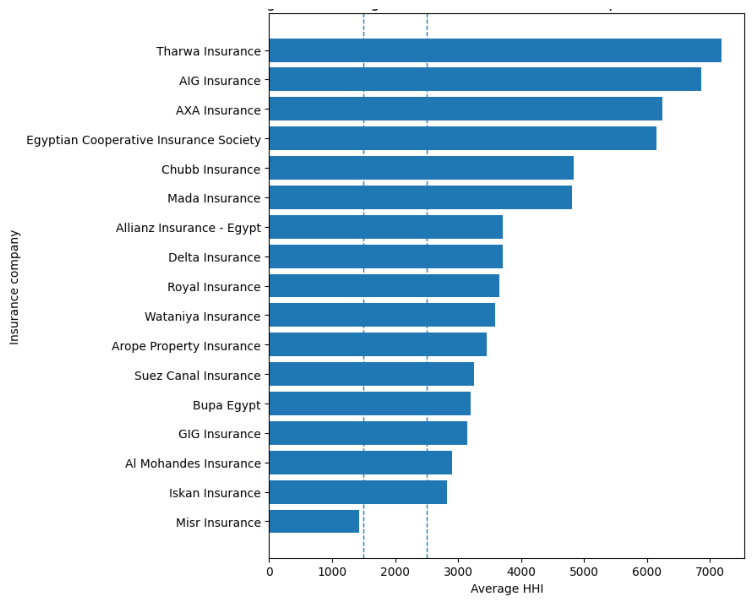
Table 1.
Descriptive Statistics of the Study Variables.
| Variable | Mean | Median | Std. Dev. | Skewness | Kurtosis | Jarque–Bera | Prob. |
| HHI | 3906 | 3574 | 2091.20 | 0.35 | 3.20 | 1.90 | 0.39 |
| ROA | 0.06 | 0.06 | 0.04 | −0.64 | 4.01 | 9.38 | 0.01 |
| ROE | 0.16 | 0.16 | 0.18 | −1.96 | 17.20 | 768.41 | 0.00 |
| Current Ratio | 3.90 | 3.02 | 2.40 | 1.57 | 5.74 | 61.46 | 0.00 |
| Cash Ratio | 0.19 | 0.11 | 0.24 | 3.63 | 21.09 | 1345.94 | 0.00 |
| D/E | 2.20 | 1.75 | 1.96 | 2.22 | 8.63 | 182.18 | 0.00 |
| TD/TA | 0.60 | 0.64 | 0.18 | −0.90 | 4.41 | 18.46 | 0.00 |
| SER | 0.38 | 0.36 | 0.17 | 0.12 | 2.86 | 0.26 | 0.88 |
| SIZE | 6.01 | 6.09 | 1.08 | −3.88 | 23.63 | 1721 | 0.00 |
| GROWTH | 0.36 | 0.30 | 0.23 | 0.67 | 2.69 | 6.68 | 0.04 |
| AGE | 26.12 | 22.00 | 21.14 | 1.31 | 4.89 | 37.19 | 0.00 |
| LOSS | 46.82 | 49.40 | 19.72 | −0.64 | 3.89 | 8.53 | 0.01 |
| EXPR | 12.15 | 10.60 | 6.44 | 0.97 | 4.35 | 19.72 | 0.00 |
| RINS | 0.44 | 0.36 | 0.26 | 1.04 | 4.51 | 23.37 | 0.00 |
| INV | 0.10 | 0.11 | 0.04 | −0.13 | 3.30 | 0.56 | 0.76 |
Source: Authors’ calculations based on EViews output.
Table 2.
Correlation Matrix of the Study Variables.
| Variable | HHI | ROA | ROE | CASH | CR | D/E | TD/TA | SER | SIZE | GROWTH | AGE | LOSS | EXPR | RINS | INV |
| HHI | 1.000 | ||||||||||||||
| ROA | −0.098 | 1.000 | |||||||||||||
| ROE | −0.079 | 0.789 | 1.000 | ||||||||||||
| CASH | 0.112 | −0.195 | −0.180 | 1.000 | |||||||||||
| CR | 0.147 | 0.062 | −0.158 | 0.306 | 1.000 | ||||||||||
| D/E | 0.227 | −0.228 | −0.012 | −0.179 | −0.259 | 1.000 | |||||||||
| TD/TA | 0.203 | 0.073 | 0.270 | −0.286 | −0.236 | 0.785 | 1.000 | ||||||||
| SER | 0.047 | 0.131 | −0.163 | 0.426 | 0.493 | −0.696 | −0.615 | 1.000 | |||||||
| SIZE | 0.044 | 0.253 | 0.178 | −0.034 | 0.162 | 0.219 | 0.523 | 0.231 | 1.000 | ||||||
| GROWTH | 0.268 | −0.010 | 0.037 | −0.050 | −0.368 | −0.048 | 0.090 | 0.122 | 0.161 | 1.000 | |||||
| AGE | −0.314 | 0.304 | 0.176 | −0.255 | −0.015 | −0.110 | 0.043 | 0.131 | 0.564 | 0.159 | 1.000 | ||||
| LOSS | −0.075 | 0.024 | −0.034 | −0.093 | 0.265 | 0.415 | 0.453 | −0.153 | 0.414 | −0.459 | −0.035 | 1.000 | |||
| EXPR | 0.405 | −0.126 | −0.073 | 0.169 | 0.064 | −0.160 | −0.013 | 0.286 | 0.046 | 0.499 | −0.098 | −0.316 | 1.000 | ||
| RINS | 0.090 | −0.049 | −0.085 | 0.155 | −0.248 | −0.275 | −0.121 | 0.379 | 0.263 | 0.775 | 0.245 | −0.480 | 0.293 | 1.000 | |
| INV | 0.237 | 0.586 | 0.432 | −0.021 | 0.225 | 0.184 | 0.302 | 0.007 | 0.260 | −0.134 | −0.044 | 0.434 | −0.001 | −0.336 | 1.000 |
Source: Authors’ calculations based on EViews output.
Table 3.
Breusch–Pagan LM Test Results.
| Dependent Variable | Statistic | p-Value | Result |
| ROA | 5.257203 | 0.0219 | RE preferred |
| ROE | 0.071802 | 0.7887 | Pooled OLS remains appropriate |
| Current Ratio | 5.455952 | 0.0195 | RE preferred |
| Cash Ratio | 12.15773 | 0.0005 | RE preferred |
| D/E | 18.78233 | 0.0000 | RE preferred |
| TD/TA | 52.66018 | 0.0000 | RE preferred |
| SER | 50.10677 | 0.0000 | RE preferred |
Source: Authors’ calculations based on EViews output.
Table 4.
Redundant Fixed Effects Test Results.
| Variable | Cross-Section F | d.f. | p-Value | Chi-Square | p-Value | Decision |
| ROA | 3.25882 | (16,60) | 0.0006 | 53.160175 | 0.0000 | FE preferred |
| ROE | 1.19977 | (16,60) | 0.2949 | 23.594770 | 0.0987 | Pooled OLS |
| Current Ratio | 3.48047 | (16,60) | 0.0002 | 55.806560 | 0.0000 | FE preferred |
| Cash Ratio | 5.62299 | (16,60) | 0.0000 | 77.866519 | 0.0000 | FE preferred |
| D/E | 6.91679 | (16,60) | 0.0000 | 88.857242 | 0.0000 | FE preferred |
| TD/TA | 10.2563 | (16,60) | 0.0000 | 112.008837 | 0.0000 | FE preferred |
| SER | 11.6094 | (16,60) | 0.0000 | 119.847469 | 0.0000 | FE preferred |
Source: Authors’ calculations based on EViews output.
Table 5.
Hausman Test Results.
| Variable | Chi-Square | d.f. | p-Value | Preferred Model |
| ROA | 15.907192 | 8 | 0.0437 | FE |
| ROE | 5.543748 | 8 | 0.6982 | RE |
| Current Ratio | 15.816961 | 8 | 0.0451 | FE |
| Cash Ratio | 87.779930 | 8 | 0.0000 | FE |
| D/E | 22.511617 | 8 | 0.0041 | FE |
| TD/TA | 8.312415 | 8 | 0.4036 | RE |
| SER | 12.089790 | 8 | 0.1472 | RE |
Source: Authors’ calculations based on EViews output.
Table 6.
Relationship between Underwriting Concentration and Financial Stability Indicators.
| Dimension | Indicator | Model | HHI Coefficient | Std. Error | t-Statistic | p-Value |
| Profitability | ROA | FE | −0.000000429 | 0.00000400 | −0.107145 | 0.9150 |
| ROE | Pooled OLS | −0.0000219 | 0.00000950 | −2.305881 | 0.0238 | |
| Liquidity | CR | FE | −0.000134 | 0.000311 | −0.430095 | 0.6687 |
| CashR | FE | −0.00000522 | 0.0000288 | −0.181610 | 0.8565 | |
| Solvency | D/E | FE | −0.0000459 | 0.000190 | −0.242331 | 0.8093 |
| TD/TA | RE | 0.00000708 | 0.00000914 | 0.774194 | 0.4412 | |
| SER | RE | −0.00000307 | 0.00000937 | −0.327716 | 0.7440 | |
| Source: Authors’ calculations based on EViews output. Note: Reported p-values are unadjusted. Because the HHI coefficient is evaluated across seven financial outcomes, a Bonferroni-adjusted 5% family-wise significance threshold of 0.0071 (0.05/7) is considered when interpreting the results. None of the HHI coefficients meets this adjusted threshold. | ||||||
Disclaimer/Publisher’s Note: The statements, opinions and data contained in all publications are solely those of the individual author(s) and contributor(s) and not of MDPI and/or the editor(s). MDPI and/or the editor(s) disclaim responsibility for any injury to people or property resulting from any ideas, methods, instructions or products referred to in the content. |
© 2026 by the authors. Licensee MDPI, Basel, Switzerland. This article is an open access article distributed under the terms and conditions of the Creative Commons Attribution (CC BY) license (http://creativecommons.org/licenses/by/4.0/).
Copyright: This open access article is published under a Creative Commons CC BY 4.0 license, which permit the free download, distribution, and reuse, provided that the author and preprint are cited in any reuse.