

Submitted:
04 October 2026
Posted:
07 October 2026
You are already at the latest version
Abstract
The conservation of industrial heritage has shifted from mere physical preservation to adaptive reuse; accurately distinguishing between historical components, later modifications, and other architectural elements is crucial for quantitative spatial analysis and renovation assessment. However, maintaining historic character often makes elements with different semantic attributes visually similar. Key challenges include subtle local differences between similar classes, insufficient coordination between local details and global context, and class imbalance causing intra-class dispersion and inter-class overlap. Using the Tianjin First Machine Tool Fac-tory as a case study, this study constructs a 14-class foreground semantic dataset and proposes Enhanced Mask2Former for Heritage Gardens (Hg-Mask2Former++). Based on Mask2Former-Swin-B, the model introduces LGFE to enhance multi-scale local–global representations and CDCC to optimize class relationships through class-balanced sampling and supervised contrastive learning. With only a 1.49% parameter increase, Hg-Mask2Former++ achieves 73.92% mIoU and 82.67% mDice, improving the baseline by 2.12 and 1.86 percentage points. Under identical experimental settings, its mIoU exceeds that of eight comparison models, including FastVim, TPSegformer, and ViT-P-based models proposed in 2026; the IoU of Industrial Building and Modern Building improves by about 20 percentage points. Further experiments reveal class-selective and condi-tion-dependent gains, indicating that scene-specific targeted optimization is more suitable than simply increasing network complexity.
Keywords:
industrial heritage
; semantic segmentation
; fine-grained recognition
; Hg-Mask2Former++
; lo-cal-global feature enhancement
; contrastive learning
1. Introduction
The preservation of industrial heritage has gradually shifted from early-stage surveys of existing structures and physical conservation toward adaptive reuse and the reconstruction of spatial value; its scope of study has also expanded from individual buildings to multi-level environments such as sites, districts, and industrial landscapes [1,2]. With the integration of computer vision technology into the study of the built environment, image-based semantic segmentation has gradually become a key method for extracting spatial elements such as roads, buildings, vegetation, and infrastructure, and is used to support quantitative analysis, visual assessment, and environmental perception analysis [3,4,5,6]. However, in the context of industrial heritage regeneration, historic industrial buildings, industrial structures, and later-added structures often share similar materials, colors, scales, and architectural languages, resulting in significant inter-class similarity among objects with different semantic attributes. Related research on fine-grained building recognition indicates that merely identifying the presence or absence of a building is no longer sufficient for further attribute analysis [7]. Therefore, as deep learning is increasingly applied to heritage research, the key challenge has shifted from coarse-grained determination of “what is present” in a scene to reliably distinguishing objects that are visually similar but differ in functional attributes and spatial semantics.
This problem encompasses three interrelated scientific questions. First, how are local variations and global context jointly represented? The discrimination of visually similar categories relies on details such as edges, textures, and component relationships; however, the same local pattern may correspond to different semantic meanings in different spatial contexts. Therefore, emphasizing either local or global information alone may lead to discrimination bias. Second, can feature enhancement truly translate into category separability? Differences in pixel-scale characteristics and occurrence frequencies across categories may lead to large-scale category-dominated gradient updates, causing difficult categories to retain significant intra-class dispersion and small inter-class distances. Finally, how can we use improvements in overall accuracy to further identify the true mechanisms and applicability boundaries of model enhancements? An increase in overall mIoU may mask a redistribution of performance across categories and fails to clarify whether the improvements act on boundaries, regional semantics, or a small number of key difficult categories.
Addressing the challenge of jointly representing local variations and global context, existing research has gradually expanded from modeling local structures to the joint representation of local and global information. Su et al. proposed a dual-local attention module to address the insufficient extraction of local neighborhood information in architectural facade point clouds, using self-attention and attention pooling to enhance the representation of local geometric structures and neighborhood context [8]. Wang et al. developed UNetFormer for remote sensing urban scenes, using a global-local Transformer module at the decoder to simultaneously model long-range context and local spatial information [9]. Building on this, Chen et al. further adopted a dual-stream architecture combining convolutional and Transformer layers, enabling the explicit extraction and interactive fusion of high-resolution local features and global contextual features in independent branches [10]. Ma and Lan, on the other hand, focused on cross-level information propagation, fusing low-level spatial details and high-level semantic information through feature reweighting and efficient attention mechanisms to improve multi-stage feature collaboration [11]. Overall, the focus of this class of research has gradually shifted from simply enhancing local information to the collaborative modeling of local details, global context, and multi-level semantics, thereby laying the foundation for further discussion on whether enhanced features can form stable class discrimination relationships. As the research focus has shifted from “how to obtain more comprehensive visual features” to “how to organize class relationships within the feature space,” contrastive learning has gradually been applied to enhance class discrimination capabilities. Addressing the challenge that single-scale pixel comparisons cannot fully capture intra-class variations, Jiang et al. extended the contrastive relationship to a multi-scale feature space, learning hierarchical intra-class consistency and inter-class separability through pixel-to-component relationships [12]. Yang et al., focusing on cross-domain architectural segmentation, combined a region-edge dual branch with difficult pixel sampling to strengthen feature alignment in boundary regions through cross-domain pixel comparisons [13]. Yuan et al. further extended the contrastive relationships to multiple levels—including images, regions, pixels, and object boundaries—to enhance the completeness and discriminative power of object features under weakly supervised conditions [14]. Building on this, Ren et al. shifted from traditional pixel-prototype comparison to prototype-pixel relationship modeling anchored by category prototypes, thereby strengthening intra-class variation and feature space organization while reducing the overhead of additional updates [15]. Chen et al. combined category-balanced threshold selection with pixel-level contrastive learning to further constrain semantic relationships among category features in a shared embedding space for labeled and unlabeled data, thereby alleviating category confusion [16]. Overall, existing research is no longer limited to basic distance constraints between positive and negative samples but, based on the discriminative challenges in different tasks, refines modeling from various perspectives, including multiscale compositional relationships, difficult boundary pixels, multilevel semantics, class prototypes, and class balance. In addition to the two main lines of research mentioned above, related studies have further focused on the model’s generalization ability and prediction reliability under conditions of changing data distributions. Rafi et al. systematically reviewed generalization methods in the semantic segmentation domain, emphasizing the models’ pixel-level prediction capabilities on unknown target domains [17]. Williams et al., on the other hand, utilized unlabeled target domain data to learn pixel-level uncertainty, thereby identifying potential segmentation errors under conditions of distribution shifts [18]. Overall, existing research has advanced the performance of semantic segmentation by addressing local-to-global feature enhancement, class relationship constraints, and cross-distribution generalization and reliability, respectively. However, these methods are primarily oriented toward scenarios such as urban remote sensing imagery and autonomous driving, and their applicability and suitability for heritage environments remain to be validated. Furthermore, there remains room for research into the role of feature enhancement and class discrimination constraints on highly confounding classes—including their combined effects—and whether these remain stable under varying structural scales, constraint strengths, and data distribution conditions.
Based on the above insights, this paper proposes two hypotheses: First, the primary bottleneck of baseline models in industrial heritage built environments is not the general failure to detect objects, but rather is more likely to be concentrated in the misclassification of categories with similar visual and semantic attributes; second, if we first enhance the joint representation of local structural differences and global context, and then further constrain the relative relationships between different categories, we can expect to form a progressive, fine-grained classification process. To validate this approach, this paper first constructs a foreground semantic dataset comprising 14 categories, including industrial buildings, industrial structures, and modern buildings, and identifies the primary bottlenecks of baseline models through multi-model comparisons, category-level IoU, Precision, Recall, confusion matrices, and analysis of typical high-error samples. Consequently, we propose Enhanced Mask2Former for Heritage Gardens (Hg-Mask2Former++), In the first stage, a Local–Global Feature Enhancement (LGFE) module is constructed. While maintaining the original four-level feature space dimensions and channel interfaces, it uses depthwise convolutions to extract local texture and structural responses, combines these with global average pooling to form channel-level context gating, and then utilizes learnable residual coefficients to adaptively control the enhancement intensity; In the second stage, we construct a Class-Discriminative Contrastive Constraint (CDCC), which acts exclusively on the `mask_features` of the Pixel Decoder during training. Through class-balanced sampling and supervised contrastive constraints, this approach enhances the consistency of features within the same class while increasing the relative separability of different classes in the feature space. Subsequently, we further validate the performance, working mechanism, and applicability boundaries of Hg-Mask2Former++ through ablation experiments, as well as analyses of structural scale and parameter responses, module interactions, interpretability, and cross-model and cross-dataset experiments.
The main contributions of this paper are threefold:
1. We constructed a fine-grained semantic segmentation dataset tailored to built environments of industrial heritage. Based on on-site panoramic images of the Tianjin First Machine Tool Factory, we established a pixel-level annotation system covering 14 semantic categories, including industrial buildings, industrial structures, and modern buildings. Building on this, we proposed a scientific workflow ranging from multi-model comparison to baseline model diagnosis, thereby shifting the model optimization focus from general overall accuracy improvement to reducing semantic misclassification between visually similar categories.
2. We propose Hg-Mask2Former++, which, with only a 1.49% increase in the number of parameters, improves mIoU from 71.80% to 73.92% and mDice from 80.81% to 82.67%, while maintaining efficiency comparable to the original baseline.
3. Through derived experiments, we further reveal that Hg-Mask2Former++ exhibits distinct category selectivity and conditional dependency; that is, there is no stable linear relationship between the number of enhanced structures, the strength of contrast constraints, and module collaboration. This indicates that fine-grained semantic segmentation of industrial heritage is better suited for targeted optimization based on scene-specific errors rather than achieving universal gains through universally transferable gains through module stacking.
2. Related Work
2.1. Research Subjects and Data Sources
Tianjin is China’s second-largest industrial city in modern times, encompassing sectors such as textiles, metals, machinery, chemicals, and printing, and holds a pivotal position in the country. As one of the “Eighteen Arhats” of New China’s machine tool industry and the birthplace of the country’s first all-gear lathe, the physical space of the Tianjin First Machine Tool Factory embodies the collective memory of New China’s industrialization and the history of its technological evolution, possessing the intrinsic value of a living industrial museum. Tianjin First Machine Tool Factory is located at the intersection of Jintang Road and Yueya River South Road in Hedong District, covering an area of approximately 281,100 square meters. The original site consisted of residential and production zones, preserving various industrial built elements such as factory buildings, workshops, and residential facilities. The urban renewal project (Jin Yi PARK), led by Tianjin TEDA Holdings in 2023, has now largely completed its transformation from an industrial rust belt into a cultural and creative industrial park. As the park is not yet fully completed, the current industrial heritage renewal efforts are primarily concentrated in the northwest area. Based on this and in conjunction with expert opinions, the main data collection route was determined, as shown in Figure 1. There are a total of 80 data collection points, spaced 25 m apart. To ensure data quality, photography of each space along the survey route was conducted on a sunny day between 10:00 a.m. and 2:00 p.m. on June 7, 2026. A DJI Osmo 360 was used, mounted on a tripod at a fixed height of 1.2 m. A total of 80 panoramic images were captured, with an output resolution of 15,520 × 7,760.
2.2. Semantic Categorization System and Data Processing
To minimize the impact of panoramic distortion on semantic segmentation, a Python script was used to map the panoramic images into four directional views—front, back, left, and right—resulting in a total of 320 images, each with a resolution of 2048×2048. Based on existing literature and the specific conditions of the industrial park, three mask categories unique to this dataset were added: industrial buildings, industrial structures, and modern buildings, bringing the total number of semantic classes to 14. The 320 images were annotated using Labelme and processed with SAM-assisted segmentation. After manual corrections, the semantic annotation was completed; the entire process took two months (June to August 2026). Subsequently, the JSON files corresponding to the annotated data were converted to the PASCAL VOC format via a script for use in segmentation tasks.
2.3. Comparison and Selection of Baseline Models
To compare the adaptability of different segmentation architectures to the dataset, we selected FCN [19], PSPNet [20], DeepLabV3+[21], SegFormer [22], Mask2Former [23], FastVim [24], TPSegformer [25], and ViT-P [26]. Some of these models utilize pre-trained backbone decoder architectures such as DINOv2 [27], ResNet [28], Swin Transformer [29], and UPerNet [30]. The comparison experiments used a uniform input size of 512×512. Here, mDice represents the average Dice coefficient across all semantic classes, calculated based on the full 15 classes (including “Background”), and is used to measure the overall overlap between the predicted and ground-truth regions; mHD95 represents the 95th percentile of the bidirectional Hausdorff distance between the predicted and ground-truth boundaries, and is used to measure the spatial boundary error in the segmentation results; “Params” refers to the total number of parameters in the complete network model; ‘GFLOPs’ are uniformly estimated using MMEngine. Models for which a complete count is not possible are denoted by “—,” and estimation results for models containing partially unsupported operators are marked with “*”. FPS, Inference Time, and Peak Mem were all tested on the same NVIDIA GeForce RTX 4090 GPU, using a fixed image size, batch size of 1, and FP32 precision, with TTA disabled. Twenty warm-up runs were performed before testing, and the average inference time and FPS were calculated based on the results of the subsequent 200 consecutive inference runs; Peak Mem is generally calculated as the peak GPU-allocated memory during the inference process. For Mask2Former-Swin-B+ViT-P (DINOv2-B), since the two stages of the model run in different dependency environments, Peak Mem was estimated based on the PyTorch peak GPU memory measured during one inference stage and the GPU memory occupied by the model parameters of the other stage; therefore, it is marked with “*”. The results are shown in Table 1.
In terms of segmentation accuracy, Mask2Former-Swin-B achieved an mIoU of 71.80%, while ViT-P (DINOv2-B) achieved an mIoU of 71.79%, which is essentially on par with its results; At the same time, Mask2Former-Swin-B achieved mDice, mAcc, and aAcc values of 80.81%, 80.83%, and 89.24%, respectively. Notably, its mDice score was also the highest among the compared models, indicating strong performance in both the quality of class region overlaps and overall recognition capability. In terms of efficiency, PSPNet achieves the fastest inference speed, while TPSegformer has the lowest number of parameters and GPU memory usage; however, the overall segmentation accuracy of both is lower than that of Mask2Former-Swin-B. Although ViT-P achieved a similar mIoU, its model size and inference overhead increased significantly. It should be noted that, to maintain a consistent input baseline with other models, ViT-P still uses 512×512 images as input; however, due to block size constraints, its classification stage performs symmetric zero-padding on the normalized 512×512 input to 518×518 before processing. Considering both accuracy and computational overhead, Mask2Former-Swin-B provides a performance foundation better suited for subsequent fine-grained diagnosis and structural improvements; therefore, it was selected as the baseline model.
2.4. Diagnosing Performance Bottlenecks at the Class Level
2.4.1. Class Performance and Confusion Relationships
The shortcomings of the baseline model in class classification are primarily concentrated in certain hard surface and architectural semantic categories. The IoU for “Road” is only 40%, while that for the visually similar “Pavement” reaches 86.96%; “Industrial Building” and “Modern Building” achieved 56.52% and 54.40%, respectively, but “Industrial Structure” still reached 73.62%. This indicates that the model’s shortcomings are not widespread across the man-made built environment but are primarily concentrated among categories with similar visual and semantic attributes. Further analysis from an internal model perspective identifies three descriptive performance tiers: high, medium, and low, as shown in Table 2. The baseline model exhibits a relatively pronounced imbalance in performance across different semantic categories. High-level categories indicate that the model is already capable of forming stable semantic representations for certain natural elements, while low-level categories corroborate the aforementioned recognition shortcomings in categories such as “Road,” “Industrial Building,” and “Modern Building.” However, the descriptive classification alone cannot determine whether the performance decline stems from missed detections, false positives, or confusion between specific semantic categories. Therefore, it is necessary to construct a confusion matrix based on the validation set’s prediction results and diagnose the primary misclassification directions and their sources of error by combining Precision and Recall.
The confusion matrix lists the ground truth classes as rows and the predicted classes as columns, with rows normalized by ground truth class. The figure omits the “Background” class and labels only the major off-diagonal entries with misclassification rates of at least 3%; the results are shown in Figure 2. A total of 9 sets of off-diagonal misclassification relationships were identified, involving 7 ground truth classes: Road, Pavement, Industrial Building, Industrial Structure, Modern Building, Bare Soil, and Facility. First, among the hard surface classes, there is a clear asymmetric confusion between “Road” and “Pavement”: 41.59% of “Road” pixels were misclassified as “Pavement,” while only 3.57% of “Pavement” pixels were misclassified as “Road.” Second, the building classes also exhibit bidirectional confusion: 30.70% of “Modern Building” pixels were misclassified as “Industrial Building,” while the reverse misclassification rate was 11.59%; The relatively low Precision of “Industrial Building” further indicates a substantial number of false positives originating from other classes. Additionally, “Bare Soil” primarily exhibits concentrated confusion with “Grass,” while “Facility” has a Recall of 75.31%, with 8.64% of true pixels misclassified as “Pavement” and another 5.81% classified as “Modern Building,” indicating that “Facility” targets are subject to multi-directional semantic interference. Based on a comprehensive analysis of category performance and confusion relationships, Road, Industrial Building, Modern Building, Bare Soil, and Facility were ultimately identified as the priority performance bottleneck categories.
2.4.2. Spatial Distribution of Typical High-Error Samples
Confusion matrices and category-level metrics can reveal the relationships between different semantic categories at the overall level, but they cannot further reflect the distribution patterns of errors in specific spatial contexts—that is, they cannot determine whether the decline in category performance is primarily due to local deviations near the target boundaries or to regional-level semantic substitutions over a larger area. Therefore, representative misclassification samples were selected for spatial-level diagnosis. Among these, the “Road—Pavement” pair corresponds to the most prominent hard-surface confusion relationship mentioned earlier, while “Industrial Building—Modern Building” exhibits bidirectional architectural category confusion; furthermore, “Road,” “Industrial Building,” and “Modern Building” all belong to the low-level categories mentioned previously. Consequently, this paper selects these three as representative cases, designating the sample with the highest number of erroneous pixels for the target class in the validation set as “rank 1” for each. By comparing the original images, ground truth annotations, model predictions, and regions with incorrect target class labels, we further analyze the spatial manifestations of major misclassifications, as shown in Figure 3. In the three typical “rank 1” samples, the FN rates for the target classes Road, Industrial Building, and Modern Building all reached 100%. Specifically, in 050.jpg_Right, 94.99% of the “Road” pixels were misclassified as “Pavement”; in 044.jpg_Front, 99.22% of the “Industrial Building” pixels were misclassified as “Modern Building”; and in 018.jpg_Back, 99.16% of the “Modern Building” pixels were misclassified as “Industrial Building,” with the misclassification direction consistent with the overall confusion matrix of the validation set. Category performance, confusion matrices, and representative samples collectively indicate that the performance limitations of the baseline model are not limited to category shifts near the edges but extend to misclassifications of category attributes over a broader range. Therefore, future improvements should further strengthen the collaborative representation of local differences and scene context to lay the foundation for enhancing the distinguishability of similar categories.
3. A Two-Stage Enhancement Method for Fine-Grained Semantic Segmentation
3.1. Overall Model Framework
The aforementioned analysis indicates that the baseline model demonstrates good overall semantic segmentation performance in the Jin Yi Park dataset; however, its primary performance bottleneck is not general object omission or boundary displacement, but rather confusion between classes with similar visual attributes. Relying solely on the original multiscale semantic modeling remains insufficient for establishing stable, fine-grained class boundaries. Based on this, Hg-Mask2Former++ builds upon Mask2Former-Swin-B, retaining its core encoding and decoding framework, while implementing incremental enhancements at both the feature representation and class relationship constraint levels to minimize disruption to the original model structure and inference process. As shown in Figure 4, the input image first undergoes four layers of feature extraction via the Swin-B backbone network, with channel counts of 128, 256, 512, and 1024, respectively. Subsequently, an LGFE Neck is inserted between the backbone and the Mask2Former head to perform independent local-to-global feature enhancement on the four-level features, while preserving the spatial dimensions and channel counts of features at each scale—rather than performing serial computations across different scales. The enhanced features are then fed into the original Mask2Former’s MSDeformAttn Pixel Decoder, yielding three levels of `multi_scale_memorys` and `mask_features` at 1/4 scale with 256 channels; the former participates in multi-scale query interactions within the Transformer Decoder, while the latter is used to generate mask predictions. The overall feature propagation process can be represented as:
In this equation, I represents the input image; (·) denotes the Swin-B backbone; represents the features at level i after LGFE enhancement; M denotes the mask_features output by the Pixel Decoder; and Pl denotes the 3-level multi_scale_memorys. In the actual code, the Pixel Decoder returns both types of features simultaneously; the three-level memory features are projected, hierarchically embedded, and position-encoded before entering the Transformer Decoder. Building on this, a CDCC branch—activated only during training—is further derived from M to use true semantic labels to guide category-balanced feature sampling and supervised contrastive constraints. This branch does not introduce a new inference path, so the inference stage continues to follow the main Mask2Former workflow enhanced by LGFE. This forms a two-stage improvement logic of “local–global feature enhancement and category discrimination constraints”: the former improves the feature representation fed into the decoder, while the latter further constrains the intra-class and inter-class relationships in the feature space.
3.2. Local-Global Feature Enhancement Module (LGFE)
3.2.1. Local-Global Dual-Branch Feature Modeling
Local branches are primarily used to enhance texture, edges, and local structural information within the neighborhood. For the input feature at the i-th scale of Swin-B, let , where Ci ∈ {128,256,512,1024}. The local branch first employs 3×3 depthwise convolutions to extract local spatial responses, preserving neighborhood structural information with low parameter overhead; Subsequently, GroupNorm and the GELU activation function are applied to perform feature normalization and nonlinear mapping, and 1×1 convolutions are used to facilitate information exchange between channels. This process can be represented as:
Li(Xi) = GN[Conv1×1(GELU[GN(DWConv3×3(Xi))])]
In parallel with the local branch, the global context branch is used to extract channel-level semantic information from the overall feature response. This branch first performs global average pooling on Xi to compress the spatial dimension into a global channel description; it then performs channel compression and restoration through two layers of 1×1 convolutions, and generates channel-level context weights via a Sigmoid function. The process can be represented as follows:
In this case, the channel compression ratio is set to r=16. In the specific implementation, to prevent low-channel-scale features from resulting in an overly narrow intermediate representation after compression, the number of intermediate channels is defined as:
Therefore, the number of intermediate channels corresponding to the four-level input features are 16, 16, 32, and 64, respectively. This configuration limits the scale of additional parameters while preserving the necessary channel mapping capacity for different scales. This yields, respectively, the local feature responses Li(Xi) and the channel-level context gating Gi(Xi), which serve as inputs for subsequent adaptive fusion.
3.2.2. Adaptive Residual Fusion and Multiscale Access
To adaptively recalibrate local responses using the global context and further control the strength of the enhancement information’s effect on the original features, a learnable scalar γi is introduced, and the enhanced output at the i-th scale is obtained through a residual connection:
Yi = Xi + γi [Li (Xi )⊙Gi (Xi )]
In the equation, ⊙ denotes element-wise multiplication; Li(Xi) represents the local feature response extracted by the local branch; Gi(Xi) represents the channel-level gating weights generated by the global context branch; and γi is a learnable scalar independently set for the i-th LGFE block. In the specific implementation, γi is initialized to 0; therefore, during the initial training phase, Yi = Xi, ensuring that the newly added module initially maintains an approximately identity mapping. As parameters are updated, γi gradually learns, via backpropagation, the contribution strength of the feature enhancement term in the residual branch, thereby adaptively introducing enhancement information while preserving the original backbone features.
The four LGFE blocks correspond one-to-one with the four levels of backbone features. After independent enhancement at each scale, the results are fed as a whole into the subsequent Mask2Former head in the form of Y1 ,Y2 ,Y3 ,Y4.
3.3. Class-Discriminative Contrastive Constraint (CDCC)
3.3.1. Category-Balanced Feature Sampling
The CDCC acts directly on the `mask_features` output by the Pixel Decoder. To establish a correspondence between pixel features and true semantic classes, we first use nearest-neighbor interpolation to scale the original semantic labels to the spatial resolution of `mask_features`, and then unfold the feature map into 256-dimensional pixel features based on spatial position. Next, for each image in a batch, the actually present foreground classes are identified, and up to K = 32 feature points are randomly sampled for each class. If a class has fewer than 32 valid pixels, all available features are retained. The “Background” class and invalid labels are excluded from sampling. By setting a consistent sampling upper limit for each foreground class, this approach mitigates the excessive influence that classes with a large area—due to their superior pixel count—might exert on the additional contrast constraint. After sampling is complete, the features obtained from the batch are concatenated into F ∈ ℝN×256, where N is the number of valid sampling points in the current batch that actually participate in the CDCC calculation.
3.3.2. Class-Discriminative Contrastive Loss and Joint Training Objective
The sampled features are L2 normalized, i.e., zi = fi/∥fi∥2, so that the inner product between normalized features represents their cosine similarity. Subsequently, using τ = 0.1 as the temperature parameter, positive sample relationships are established for samples of the same class, while samples of different classes are collectively included in the comparison normalization. For feature points for which no other samples of the same class exist, they are not treated as valid anchors and are excluded from the loss averaging. Let the semantic class of sample i be Yi; other sampled features sharing the same class label as i form the positive sample set P(i), while the remaining features of different classes serve as negative samples in the normalized comparison. The CDCC loss can be expressed as:
In this equation, P(i) represents the set of positive samples that share the same semantic label as anchor i, 𝒜 represents the set of valid anchors that have at least one positive sample, and τ = 0.1 is the temperature parameter. This constraint promotes the formation of more class-discriminative organizational relationships in the feature space by increasing the relative similarity among features of the same class and ensuring that features from different classes jointly participate in the comparison normalization.
Through the above constraints, features within the same class achieve higher similarity during the optimization process, while the relative distance between features of different classes is increased, thereby complementing the inter-class feature relationships that were not directly constrained by the original segmentation loss. Throughout the entire training process, CDCC participates in backpropagation alongside the original classification loss, masked cross-entropy loss, and Dice loss of Mask2Former. The overall training objective is expressed as:
total = Mask2Former + λCDCCCDCC, λCDCC = 0.1
In particular, Mask2Former retains the original training losses—such as classification, masking, and Dice—while λCDCC is the loss weight for the additional contrastive constraint. In the final model, K = 32、τ = 0.1、λCDCC = 0.1. CDCC is activated only during the training phase and does not introduce an additional inference branch.
Consequently, LGFE and CDCC complement and optimize each other at the levels of feature representation and class relationships, respectively: the former improves the local-to-global representation of multiscale visual features, while the latter further utilizes semantic labels to constrain the organization of class features during the training phase. Their actual performance gains will be further validated in subsequent ablation and extension experiments.
4. Experimental Results and Extended Validation
4.1. Experimental Setup and Overall Performance
Hg-Mask2Former++ achieved its best results after 3,000 iterations, with mIoU and mDice reaching 73.92% and 82.67%, respectively—improvements of 2.12 and 1.86 percentage points over the baseline—indicating that the two-stage improvements enhance both the overall quality of region overlap and class recognition capabilities. A further comparison of the structural complexity and inference efficiency between Hg-Mask2Former++ and the Baseline is shown in Table 3. The number of parameters in this model increased only from 106.89 M to 108.48 M, a rise of approximately 1.49%, while FPS, per-image inference time, and peak GPU memory usage all changed only slightly. Since CDCC is only involved in contrast constraints during the training phase and does not add prediction branches, the additional parameters and inference overhead primarily stem from the first-stage LGFE.
4.2. Ablation Experiments and Performance Responses at the Class Level
To identify the sources of the overall performance gains, we examined the independent effects of LGFE and CDCC separately; the results are shown in Table 4. When LGFE and CDCC were introduced individually, mIoU reached 73.41% and 73.22%, respectively—both higher than the baseline’s 71.80%—indicating that both improvements can independently contribute to performance gains. When combined to form Hg-Mask2Former++, the mIoU, mAcc, aAcc, and mDice scores all exceeded those of the single-module models. Specifically, the mIoU of Hg-Mask2Former++ increased by 0.51 and 0.70 percentage points compared to LGFE and CDCC, respectively, and mDice by 0.81 and 0.75 percentage points, respectively. However, mHD95 increased to 373.22 px, suggesting that the gains are primarily reflected in region segmentation and class recognition; therefore, it cannot be concluded that the two improvements exhibit a consistent positive additive relationship across all performance dimensions.
The results at the category level show significant selectivity, as shown in Table 5. Specifically, the IoU for “Industrial Building” and “Modern Building” increased from 56.52% and 54.40% to 76.50% and 75.79%, respectively—an increase of 19.98 and 21.39 percentage points—indicating that the overall improvement was particularly pronounced for these highly confounded building categories. The IoU for “Road” increased from 40.00% to 47.00%, but remained slightly lower than the 47.40% achieved when LGFE was applied alone, indicating that the improvement in this category primarily stemmed from the first-stage feature enhancement. Meanwhile, the IoU for “Bare Soil” and “Industrial Structure” decreased by 12.08 and 4.78 percentage points, respectively, in the Hg-Mask2Former++ model, indicating that while the two-stage improvements enhanced the classification performance for certain challenging categories, they were accompanied by a redistribution of performance across categories.
4.3. Structural Scale, Parameter Sensitivity, and Interactions
To further investigate whether the scale of the LGFE architecture, the strength of the CDCC constraint, and their interaction exhibit a stable monotonic response, the derived experiments in this section uniformly set the random seed to 1062862894 and keep `deterministic=False`, while the remaining training settings remain consistent with those described earlier. The results in this section are intended solely for analyzing scale responses, parameter sensitivity, and patterns of module interaction, and do not supersede the conclusions of the formal main experiment.
4.3.1. Effect of the Number of LGFE Blocks
To determine whether the performance gains observed in the first stage continue to accumulate as the enhancement depth increases, four conditions were set up, as shown in Figure 5. Among these, LGFE×1 indicates that each of the four feature levels passes through a single independent LGFE unit, while LGFE×2 and LGFE×3 sequentially stack two and three independent units, respectively, on each feature level—rather than simply increasing the number of processing passes at a single scale. As the number of stacked LGFE units increased, the model’s performance did not exhibit a monotonically increasing trend. The baseline achieved its best result at 16,000 iterations, while LGFE×1 reached its best result earlier, at 5,000 iterations, with mIoU improving to 73.19%. However, upon further increases to ×2 and ×3, these values dropped to 72.99% and 72.54%, respectively; LGFE×2 achieved the highest mAcc among the four groups at 82.36%, while LGFE×3’s mHD95 dropped to 319.08 px, the lowest value among the four scales. Meanwhile, the number of parameters continued to increase with stacking depth, and inference efficiency gradually declined. Therefore, LGFE×1 offers a more reasonable balance between accuracy and efficiency under the current conditions.
4.3.2. CDCC Constraint Strength Response
In this section, we keep the previously mentioned τ and K constant and only set the CDCC loss weight λ to 0.05, 0.10, and 0.20 to examine the impact of varying the strength of the class discrimination constraint on the training process and segmentation performance, as shown in Figure 6. Based on the validation curves plotted every 1,000 iterations, the Baseline achieved its best mIoU of 71.80% at 16,000 iterations; λ = 0.05 reached 72.21% at 11,000 iterations, the highest value among the three weights; λ = 0.10 achieved 71.82% at 15,000 iterations; λ = 0.20 also reached 72.19% at 11,000 iterations, differing from λ = 0.05 by only 0.02 percentage points. All groups exhibited some degree of fluctuation in the middle and late stages, rather than continuously converging unidirectionally toward higher validation metrics as the number of iterations increased. Compared to the baseline, the mAcc, aAcc, and mDice for λ = 0.05 reached 81.68%, 89.82%, and 81.17%, respectively, while mHD95 dropped to 327.30 px; λ = 0.10 yielded the lowest mHD95; and λ = 0.20 achieved 89.85% aAcc and 81.21% mDice, which were the highest values among the three configurations. Therefore, the effect of CDCC constraint strength varies across different evaluation metrics: lower weights perform better on mIoU, moderate weights show more significant improvements in extreme spatial boundary errors, while higher weights offer a slight advantage in mDice and aAcc. These differences among metrics further indicate that the role of CDCC is better understood as a regulatory constraint on class feature relationships rather than as a means to achieve linear gains by increasing loss weights. Since CDCC is only involved in the loss calculation during the training phase, the number of model parameters and inference VRAM remain constant across different weight settings; actual speed differences manifest only as minor fluctuations in runtime.
4.3.3. The Interaction Between LGFE and CDCC
To further analyze the interaction between the two improvements, we varied the CDCC weight along the horizontal axis under two conditions, LGFE OFF and LGFE ON, as shown in Figure 7(a). Under the LGFE OFF condition, as the CDCC increased from λ = 0 to 0.05 and 0.10, the mIoU changed from 71.80% to 72.21% and 71.82%, respectively; under the LGFE ON condition, it decreased from 73.19% to 71.90% and 72.11%. The two response curves exhibited distinctly non-parallel changes, while mAcc, aAcc, and mDice showed similar trends; mHD95 also exhibited responses in different directions, indicating that the inclusion of LGFE alters the way CDCC influences model performance. At the same time, the optimal iteration counts shifted from 16,000, 11,000, and 15,000 iter under the LGFE OFF condition to 5,000, 16,000, and 20,000 iter under the LGFE ON condition. Therefore, the inclusion of LGFE not only altered the magnitude of CDCC’s response to the final accuracy but also changed the training optimization path under different constraint strengths. It should be emphasized that the changes reflected in “Best Iter” are used to describe convergence behavior and are not directly equivalent to the quality of segmentation performance.
We then construct a simple additive expectation based on the results of the two modules acting independently and compare the actual combined results with it. The interaction residual here is primarily used to describe the degree of deviation of the combined results from the simple sum of the independent gains, rather than as a test of statistical significance. For metrics such as mIoU, mAcc, aAcc, and mDice—where higher values indicate better performance—a negative value indicates that the actual combined results are lower than the theoretical additive expectation; For mHD95, the direction is standardized in the visualization so that negative values also indicate an interaction response that is detrimental to the combined gain. As shown in Figure 7(b), using Baseline as the reference, the simple additive expectation is defined as: Baseline mIoU + LGFE independent gain + independent gain under the corresponding CDCC weight. Accordingly, the theoretical expected mIoU values for λ = 0.05 and 0.10 are 73.60% and 73.21%, respectively, while the actual combined results are only 71.90% and 72.11%. This indicates that the combination of the two modules is not a simple sum of independent gains but exhibits clear conditional dependence. In the main experiment, the combined model still achieved the highest mIoU of 73.92%; therefore, this controlled experiment serves to define the limits of the combined benefit rather than to negate the validity of the main model.
4.4. Analysis of Model Interpretability and Internal Mechanisms
4.4.1. Joint Visualization Analysis of Decision Responses and Attention Allocation
To further explain the spatial decision-making basis of Hg-Mask2Former++, we perform a joint visualization at two levels: output decisions and internal attention distribution. Grad-CAM++ uses the `mask_feature` from the Pixel Decoder—shared by both the Baseline and Hg-Mask2Former++—as the target feature layer, constructing class-specific responses based on the true class regions; Cross-Attention extracts the attention weights from the 8th layer of the Transformer Decoder, averages them across the eight attention heads, and aggregates the Top-5 Queries based on target class probabilities. Figure 8 presents a comparison using three representative sample sets: Industrial Building, Modern Building, and Industrial Structure. For the same sample and under the same explanation method, the Baseline and Hg-Mask2Former++ use a shared display scale; colors represent only the spatial distribution of normalized responses and are not used for an absolute intensity comparison between Grad-CAM++ and Cross-Attention.
For the two typical samples, “Industrial Building” and “Modern Building,” the single-image IoU increased from 0 to 94.92% and 95.53%, respectively. After the improvement, the Grad-CAM++ responses covered the main building structures more continuously, and the Cross-Attention shifted from scattered responses to the target areas. The results from both groups indicate that the improvement in fine-grained building category segmentation is well aligned spatially with the reorganization of target subject decision responses and internal semantic matching. For the “Industrial Structure” sample, the IoU changed by only 0.53 percentage points, and both the prediction results and the response maps for the two categories remained relatively stable. Grad-CAM++ and Cross-Attention were primarily distributed along the upper parts of industrial structures and linear components. As a control for stable responses, this sample demonstrates that the combined improvement does not simply amplify the activation intensity across all categories but exhibits distinct category-specific behavior.
4.4.2. Attribution of Multiscale Features in LGFE
To analyze how LGFE modulates intermediate features, we selected an Industrial Building sample and extracted and extracted input features Xi, local branch responses Li(Xi), global context weights Gi(Xi), modulated features Li(Xi)⊙Gi(Xi), and the actual feature change ∣Yi − Xi∣. These were combined with the residual coefficient γi and Relative L2 for a joint analysis, as shown in Figure 9. Spatial feature maps are visualized using the mean of the absolute activation across channels and are normalized independently within each map; therefore, the heatmaps are primarily used to compare response locations and spatial patterns, rather than to determine absolute feature intensities across different scales. Results across the four scales show that the effect of LGFE exhibits distinct hierarchical differences: Stage 1 exhibits the highest residual coefficients and actual feature changes, with responses primarily concentrated at building edges and fine-grained structures; Stage 3 follows, while Stage 2 and Stage 4 produce only weak adjustments, with Stage 2 exhibiting a slight negative modulation. This indicates that LGFE does not amplify features across all levels simultaneously but rather forms an adaptive enhancement mechanism dominated by shallow, high-resolution features, with auxiliary modulation from mid-to-high levels.
4.5. Generalization Validation
In cross-model experiments, LGFE was integrated into both SegFormer (a Transformer-based architecture) and DeepLabV3+ (a CNN-based architecture). Given the strong association between CDCC and the query-based category prediction structure of Mask2Former, forced transfer was not applied to them in this section; DeepLabV3+ employed Selective-LGFE based on the actual feature propagation path. As shown in Table 6(a), the benefits of LGFE are architecture-dependent: when integrated with SegFormer, mIoU decreases by 0.28 percentage points, but mHD95 decreases by 14.72 px; when integrated with DeepLabV3+, mIoU increases by 0.51 percentage points, and mHD95 decreases by 30.35 px. This indicates that LGFE can adapt to different networks, but its benefits do not result in consistent improvements across all metrics. Further, when Hg-Mask2Former++ was transferred to Cityscapes, the results shown in Table 6(b) indicate that its mIoU improved by 0.59 percentage points and mDice by 0.38 percentage points compared to the baseline, but mHD95 increased by 2.00 px. This suggests that the model still maintains a certain level of segmentation gain across different data distributions, but its boundary performance did not improve accordingly. Overall, the proposed method demonstrates a certain degree of cross-architecture adaptability and cross-dataset transferability; however, the specific gains are still influenced by the network architecture, and it is not appropriate to infer that it possesses universal advantages across all scenarios.
5. Discussion and Limitations
Classification analysis by Tianjin First Machine indicates that semantic segmentation within the built environment of industrial heritage cannot be simply equated with the extraction of general environmental features. This distinction holds direct practical significance: if segmentation results containing systematic confusion are directly applied to analyses of area proportions, spatial composition, or comparisons between pre- and post-renovation states, initial classification errors may propagate into subsequent quantitative analyses. Therefore, before integrating semantic segmentation results into heritage assessment and decision-support systems, identifying and mitigating directional confusion between key categories is more critical—and warrants greater attention—than merely pursuing high overall accuracy.
Experimental results from Hg-Mask2Former++ indicate that the improvement in fine-grained discriminative ability is not a uniform benefit resulting from increased network complexity, but rather resembles a reorganization of the relationship between feature representations and classes. First, LGFE essentially reweights the backbone features; while a single-stage enhancement may help highlight differences in local structure and global context, continuous stacking may repeatedly disrupt the hierarchical representations already formed by the original Swin-B. Consequently, as the network scale continues to increase, the number of parameters and computational burden rise continuously, while effective discriminative information does not necessarily increase in tandem. Previous studies have similarly found that the continuous stacking of feature enhancement modules may reduce generalization performance due to increased network complexity and overfitting, which aligns with the non-monotonic response observed in this study [31]. Second, CDCC itself is not an independent prediction module but rather an additional constraint during the training phase that alters the organization of the feature space; if the constraint is too weak, adjustments to class relationships are limited, while if it is too strong, it may compete with the original objective. In particular, differences among classes in terms of area proportion, intra-class variation, and visual similarity further amplify this unbalanced response, which explains why some highly ambiguous building classes show significant improvement, while other classes and boundary metrics do not benefit to the same extent. Related studies have also indicated that overly strong contrast constraints may interfere with the primary segmentation task, consistent with the weight sensitivity results in this paper [32]. In contrast, some studies have reported sustained complementary gains following the integration of multiple modules [33], which differs from the results of this paper’s controlled experiments, where no stable positive synergy was observed. This suggests that module synergy is likely task-dependent and may be jointly influenced by data distribution and semantic structure.
This study has certain limitations: First, the design and experiments were conducted within a purely supervised framework. In future work, we intend to employ semi-supervised methods [34], specifically using semi-supervised data augmentation to incorporate data from diverse distributions—thereby broadening the dataset's coverage and reducing reliance on manual annotation. Secondly, this paper does not discuss different loss functions; the choice of loss function determines the direction and focus of model optimization [35]. In future work, we will examine various loss functions and conduct a more detailed analysis of issues such as class imbalance, small-object segmentation, and boundary ambiguity.
6. Conclusions
This study focuses on the problem of fine-grained semantic confusion among visually similar categories in the context of industrial heritage revitalization. With only a small increase in the number of parameters, Hg-Mask2Former++ significantly improved the recognition of multiple sets of highly confounding categories. Further results indicate that the improvement in model performance stems primarily from targeted adjustments to the discriminative relationships between key categories, rather than from synchronous improvements across all categories and evaluation metrics resulting from increased network complexity. Consequently, the optimization of fine-grained semantic segmentation for industrial heritage should shift from general model enhancement to targeted modeling based on specific error structures. This approach enhances the reliability of pixel-level differentiation among built elements with distinct historical attributes, thereby providing a more stable data foundation for quantifying spatial composition and evaluating renovations in downstream tasks. Particularly in scenarios where heritage preservation and reuse coexist, distinguishing elements with different attributes but similar visual appearances helps prevent coarse-grained statistical analysis from obscuring the differences between old and new elements.
Author Contributions
Conceptualization, K.L. and X.G.; methodology, K.L., X.G., C.X. and G.F.M.; software, K.L.; validation, K.L., X.S. and S.M.; investigation, K.L., X.S., C.X. and S.M.; data curation, K.L. and S.M.; writing—original draft preparation, K.L.; writing—review and editing, X.G., C.X. and G.F.M.; supervision, X.G., C.X. and G.F.M. funding acquisition, X.G. All authors have read and agreed to the published version of the manuscript.
Funding
This research received no external funding.
Data Availability Statement
The data presented in this study will be made publicly available in an open repository. The repository name and access link will be provided during the review process.
Conflicts of Interest
The authors declare no conflicts of interest.
Abbreviations
The following abbreviations are used in this manuscript:
| Hg-Mask2Former++ | Enhanced Mask2Former for Heritage Gardens |
| LGFE | Local–Global Feature Enhancement |
| CDCC | Class-Discriminative Contrastive Constraint |
| IoU | Intersection over Union |
| mIoU | Mean Intersection over Union |
| mAcc | Mean Accuracy |
| aAcc | All Accuracy |
| mDice | Mean Dice Coefficient |
| mHD95 | Mean 95th-Percentile Hausdorff Distance |
| GFLOPs | Giga Floating-Point Operations |
| FPS | Frames Per Second |
| TTA | Test-Time Augmentation |
| SAM | Segment Anything Model |
References
- TICCIH. The Nizhny Tagil Charter for the Industrial Heritage. TICCIH 2003. [Google Scholar]
- ICOMOS; TICCIH. Joint ICOMOS–TICCIH Principles for the Conservation of Industrial Heritage Sites, Structures, Areas and Landscapes (The Dublin Principles); Adopted by the 17th ICOMOS General Assembly. 28 November 2011. [Google Scholar]
- Zhang, Y.; Gao, J.; Yang, M.; Zhang, B.; Li, H.; Zhai, F. Optimization strategy for coal mine industrial heritage renewal based on semantic segmentation and postoccupancy evaluation of street view images: A case study of the Wangfeng Mine in Jiaozuo city. J. Asian Archit. Build. Eng. 2025, 1–18. [Google Scholar] [CrossRef]
- Shi, J.; Mei, L.; Meng, Y.; Gao, W. Revealing the relationship between urban park landscape features and visual aesthetics by deep learning-driven and spatial analysis. Buildings 2025, 15, 2487. [Google Scholar] [CrossRef]
- Wang, Y.; Wang, S.; Pan, Y.; Li, C.; Chen, C.; Wang, J. Immersive virtual reality and computer vision for heritage: Visual evaluation and perception of the industrial heritage sites along the Yunnan–Vietnam railway (Yunnan section). Herit. Sci. 2024, 12. [Google Scholar] [CrossRef]
- Meng, X.; Chang, J. Sustainable reuse evaluation framework for coastal industrial living preservation of heritage buildings based on visual perception driven. Sci. Rep. 2025, 15. [Google Scholar] [CrossRef] [PubMed]
- Li, W.; Yu, J.; Chen, D.; Lin, Y.; Dong, R.; Zhang, X.; He, C.; Fu, H. Fine-grained building function recognition with street-view images and GIS map data via geometry-aware semi-supervised learning. Int. J. Appl. Earth Obs. Geoinf. 2025, 137, 104386. [Google Scholar] [CrossRef]
- Su, Y.; Liu, W.; Yuan, Z.; et al. DLA-Net: Learning dual local attention features for semantic segmentation of large-scale building facade point clouds. Pattern Recognit. 2022, 123, 108372. [Google Scholar] [CrossRef]
- Wang, L.; Li, R.; Zhang, C.; Fang, S.; Duan, C.; Meng, X.; Atkinson, P.M. UNetFormer: A UNet-like transformer for efficient semantic segmentation of remote sensing urban scene imagery. ISPRS J. Photogramm. Remote Sens. 2022, 190, 196–214. [Google Scholar] [CrossRef]
- Chen, M.; Zhang, L.; Feng, R.; et al. Rethinking local and global feature representation for dense prediction. Pattern Recognit. 2023, 135, 109168. [Google Scholar] [CrossRef]
- Ma, Y.; Lan, X. Semantic segmentation using cross-stage feature reweighting and efficient self-attention. Image Vis. Comput. 2024, 145, 104996. [Google Scholar] [CrossRef]
- Jiang, J.; et al. Hierarchical contrastive learning for semantic segmentation. IEEE Trans. Neural Netw. Learn. Syst. 2024, 36, 11202–11214. [Google Scholar] [CrossRef] [PubMed]
- Yang, M.; et al. Unsupervised domain adaptive building semantic segmentation network by edge-enhanced contrastive learning. Neural Netw. 2024, 179, 106581. [Google Scholar] [CrossRef] [PubMed]
- Yuan, K.; Schaefer, G.; Lai, Y.-K.; Wang, Y.; Liu, X.; Guan, L.; Fang, H. A multi-strategy contrastive learning framework for weakly supervised semantic segmentation. Pattern Recognit. 2023, 137, 109298. [Google Scholar] [CrossRef]
- Ren, Q.; Lu, S.; Mao, Q.; et al. Exploring prototype-anchor contrast for semantic segmentation. IEEE Trans. Circuits Syst. Video Technol. 2024, 34, 7106–7120. [Google Scholar] [CrossRef]
- Chen, J.; Chen, G.; Zhang, L.; et al. Category-sensitive semi-supervised semantic segmentation framework for land-use/land-cover mapping with optical remote sensing images. Int. J. Appl. Earth Obs. Geoinf. 2024, 134, 104160. [Google Scholar] [CrossRef]
- Rafi, T.H.; Mahjabin, R.; Ghosh, E.; et al. Domain generalization for semantic segmentation: A survey. Artif. Intell. Rev. 2024, 57, 247. [Google Scholar] [CrossRef]
- Williams, D.S.W.; De Martini, D.; Gadd, M.; et al. Mitigating distributional shift in semantic segmentation via uncertainty estimation from unlabeled data. IEEE Trans. Robot. 2024, 40, 3146–3165. [Google Scholar] [CrossRef]
- Long, J.; Shelhamer, E.; Darrell, T. Fully convolutional networks for semantic segmentation. In Proceedings of the IEEE Conference on Computer Vision and Pattern Recognition (CVPR), 2015; pp. 3431–3440. [Google Scholar]
- Zhao, H.; Shi, J.; Qi, X.; Wang, X.; Jia, J. Pyramid scene parsing network. In Proceedings of the IEEE Conference on Computer Vision and Pattern Recognition (CVPR), 2017; pp. 2881–2890. [Google Scholar]
- Chen, L.-C.; Zhu, Y.; Papandreou, G.; Schroff, F.; Adam, H. Encoder-decoder with atrous separable convolution for semantic image segmentation. In Proceedings of the European Conference on Computer Vision (ECCV), 2018; pp. 801–818. [Google Scholar]
- Xie, E.; Wang, W.; Yu, Z.; Anandkumar, A.; Alvarez, J.M.; Luo, P. SegFormer: Simple and efficient design for semantic segmentation with transformers. Adv. Neural Inf. Process. Syst. 2021, 34. [Google Scholar]
- Cheng, B.; Misra, I.; Schwing, A.G.; Kirillov, A.; Girdhar, R. Masked-attention mask transformer for universal image segmentation. In Proceedings of the IEEE/CVF Conference on Computer Vision and Pattern Recognition (CVPR), 2022; pp. 1290–1299. [Google Scholar]
- Kapse, S.; Betz, R.; Sivanandan, S. Fast Vision Mamba: Pooling spatial dimensions for accelerated processing. In Proceedings of the IEEE/CVF Winter Conference on Applications of Computer Vision (WACV), 2026; pp. 2923–2933. [Google Scholar]
- Xu, L.; Li, G.; Song, Y.; Ji, X. Hilbert curve-based attention enabling topology-preserving image tensor representation for semantic segmentation network. In Proceedings of the IEEE/CVF Conference on Computer Vision and Pattern Recognition (CVPR), 2026; pp. 13113–13122. [Google Scholar]
- Shahabodini, S.; Mansoori, M.; Bayatmakou, F.; Abouei, J.; Plataniotis, K.N.; Mohammadi, A. The missing point in vision transformers for universal image segmentation. In Proceedings of the IEEE/CVF Conference on Computer Vision and Pattern Recognition (CVPR), 2026; pp. 6314–6324. [Google Scholar]
- Oquab, M.; Darcet, T.; Moutakanni, T.; Vo, H.V.; Szafraniec, M.; Khalidov, M.; Fernandez, P.; Haziza, D.; Massa, F.; El-Nouby, A.; Assran, M.; Ballas, N.; Galuba, W.; Howes, R.; Huang, P.-Y.; Li, S.-W.; Misra, I.; Rabbat, M.; Sharma, V.; Synnaeve, G.; Xu, H.; Jégou, H.; Mairal, J.; Labatut, P.; Joulin, A.; Bojanowski, P. DINOv2: Learning robust visual features without supervision. In Mach. Learn. Res.; 2024. [Google Scholar]
- He, K.; Zhang, X.; Ren, S.; Sun, J. Deep residual learning for image recognition. In Proceedings of the IEEE Conference on Computer Vision and Pattern Recognition (CVPR), 2016; pp. 770–778. [Google Scholar]
- Liu, Z.; Lin, Y.; Cao, Y.; Hu, H.; Wei, Y.; Zhang, Z.; Lin, S.; Guo, B. Swin Transformer: Hierarchical vision transformer using shifted windows. In Proceedings of the IEEE/CVF International Conference on Computer Vision (ICCV), 2021; pp. 10012–10022. [Google Scholar]
- Xiao, T.; Liu, Y.; Zhou, B.; Jiang, Y.; Sun, J. Unified perceptual parsing for scene understanding. In Proceedings of the European Conference on Computer Vision (ECCV), 2018; pp. 418–434. [Google Scholar]
- Yang, S.; Hou, M.; Li, S. Point cloud semantic segmentation of grotto scenes using the knowledge-guided deep learning method. Int. J. Digit. Earth 2024, 17, 2385081. [Google Scholar] [CrossRef]
- Liu, Y.; Yang, Y.; Jiang, Y.; Zhao, X.; Xie, Z. FAUDA-Net: Frequency-aware unsupervised domain adaptation network for multimodal medical image segmentation. Comput. Med. Imaging Graph. 2026, 127, 102684. [Google Scholar] [CrossRef] [PubMed]
- Chen, N.; Yang, R.; Zhao, Y.; Dai, Q.; Wang, L. Remote sensing image segmentation network that integrates global–local multi-scale information with deep and shallow features. Remote Sens. 2025, 17, 1880. [Google Scholar] [CrossRef]
- Liu, X.; Guo, X. U-GANs: Pyramidal Convolutional Attention Fusion Network for Pneumonia Infection Segmentation with Semi-supervised Learning. In Advanced Intelligent Computing Technology and Applications. ICIC 2025. Communications in Computer and Information Science; Huang, D.S., Li, B., Chen, H., Zhang, C., Eds.; Springer: Singapore; vol 2564. [CrossRef]
- Xin, G.; Malykhina, G.F. Optimisation of Lung Disease Detection Algorithm Based on Yolo V8. In Advances in Neural Computation, Machine Learning, and Cognitive Research VIII. NI 2024. Studies in Computational Intelligence; Redko, V., Yudin, D., Dunin-Barkowski, W., Kryzhanovsky, B., Tiumentsev, Y., Eds.; Springer: Cham; vol 1179. [CrossRef]
Figure 1.
Schematic of the Jin Yi Park site plan and image data collection.
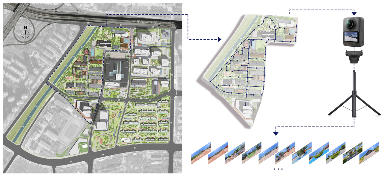
Figure 2.
Confusion matrix for the validation set of the baseline model.
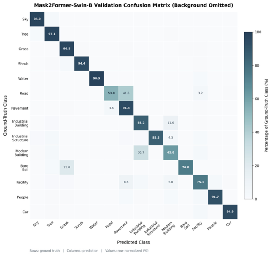
Figure 3.
Statistics on Representative Misclassified Samples from the Baseline Model.
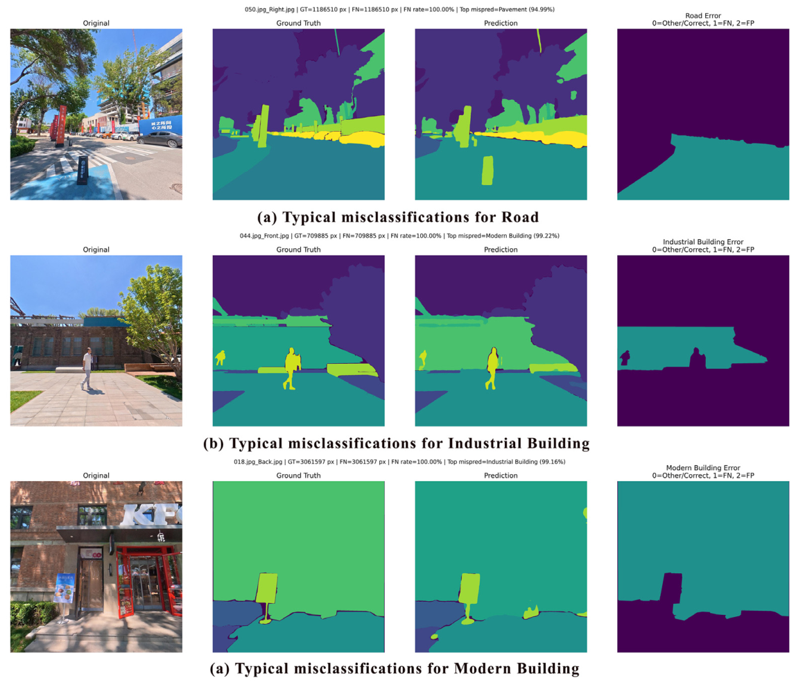
Figure 4.
Architecture of the Hg-Mask2Former++ Model.
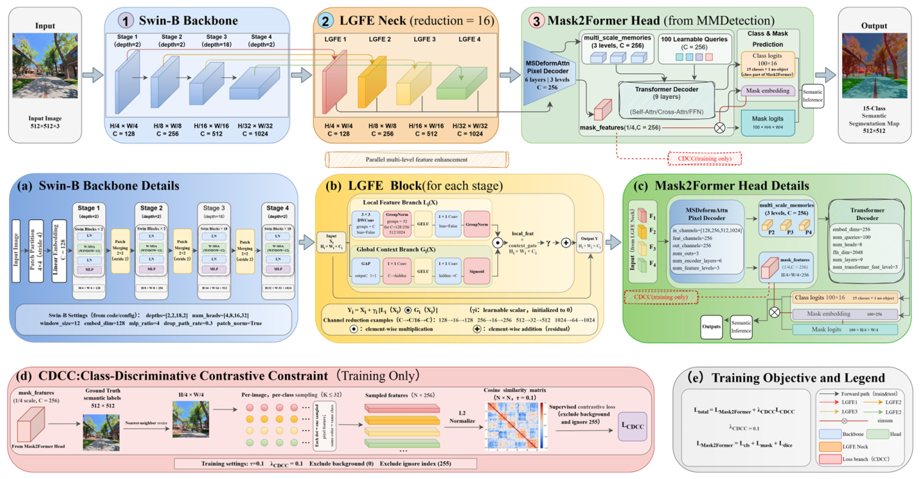
Figure 5.
Segmentation Performance Response for Different Numbers of LGFEs.
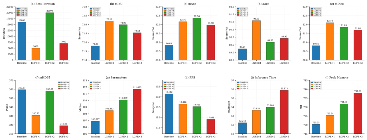
Figure 6.
Response of training and segmentation performance under different CDCC constraint strengths.
Figure 6.
Response of training and segmentation performance under different CDCC constraint strengths.
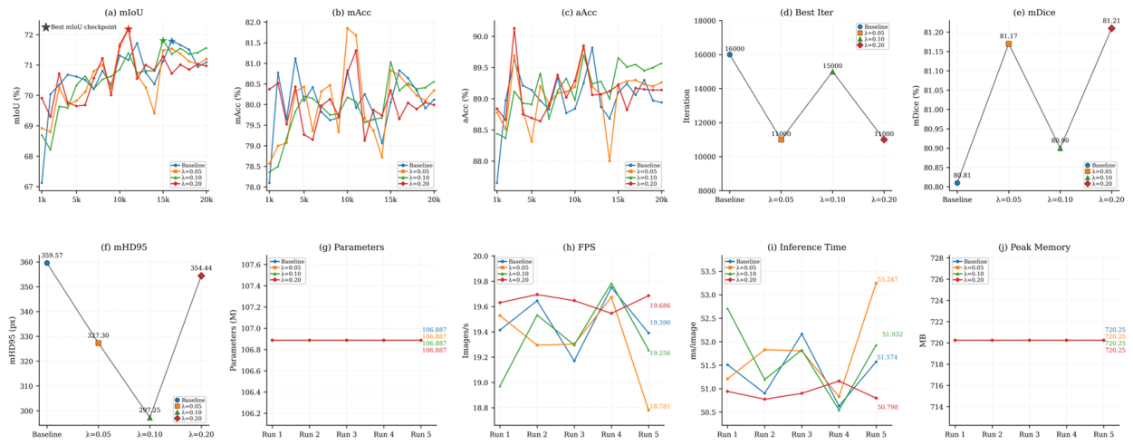
Figure 7.
Interactive responses, quantitative effects, and additive decomposition of mIoU between LGFE and CDCC.
Figure 7.
Interactive responses, quantitative effects, and additive decomposition of mIoU between LGFE and CDCC.
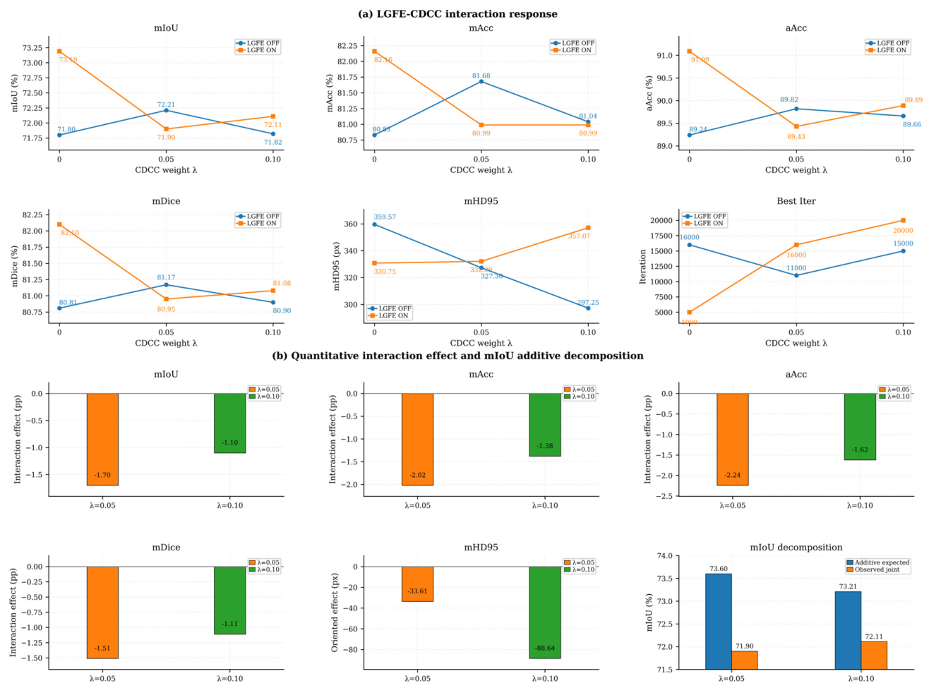
Figure 8.
Joint visualization of sample decision responses and attention allocation.
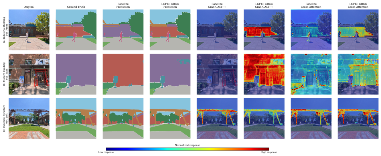
Figure 9.
Analysis of Four-Scale Feature Attribution and Residual Modulation Responses for LGFE.
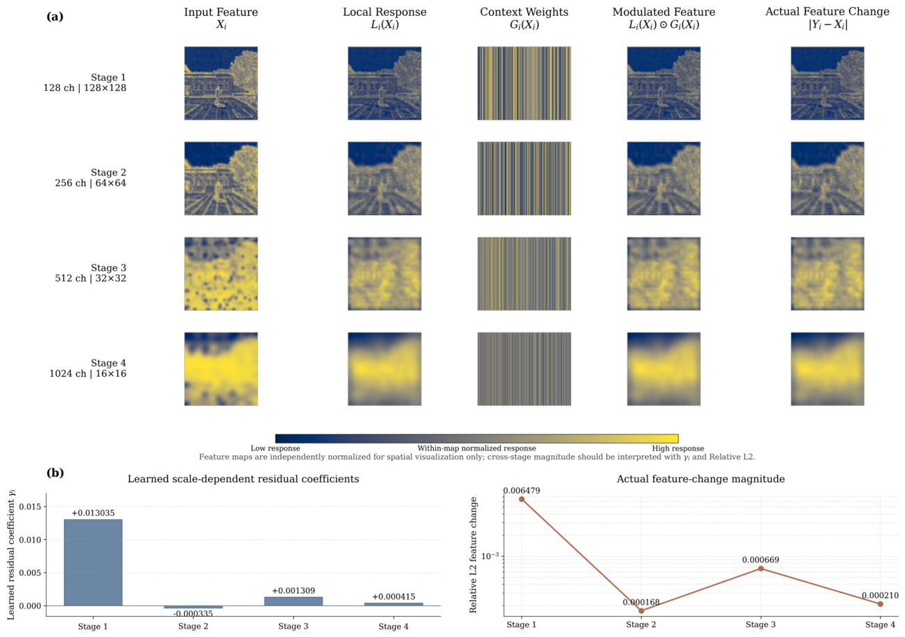

Table 1.
Segmentation Accuracy and Computational Efficiency of Different Semantic Segmentation Models.
Table 1.
Segmentation Accuracy and Computational Efficiency of Different Semantic Segmentation Models.
| Model | Best Iter | mIoU↑ (%) | mAcc↑ (%) | aAcc↑ (%) | mDice↑ (%) | mHD95↓ (px) | Params↓ (M) | GFLOPs↓ | FPS↑ | Inference Time↓ (ms/image) | Peak Mem↓ (MB) |
|---|---|---|---|---|---|---|---|---|---|---|---|
| FCN-R101 | 16000 | 68.40 | 78.04 | 88.93 | 78.06 | 385.01 | 68.49 | 276.00 | 61.62 | 16.23 | 553.99 |
| PSPNet-R101 | 12000 | 69.34 | 80.48 | 88.75 | 78.85 | 424.62 | 67.97 | 256.00 | 63.76 | 15.68 | 551.00 |
| DeepLabV3+-R101 | 19000 | 68.49 | 78.58 | 88.80 | 78.48 | 393.98 | 62.58 | 254.00 | 60.78 | 16.45 | 531.53 |
| SegFormer-B5 | 17000 | 69.63 | 78.53 | 89.21 | 78.94 | 367.99 | 81.97 | 74.61* | 29.95 | 33.39 | 616.72 |
| Mask2Former-Swin-B | 16000 | 71.80 | 80.83 | 89.24 | 80.81 | 359.57 | 106.89 | — | 26.65 | 37.52 | 720.25 |
| FastVim-B+UPerNet | 13000 | 67.27 | 77.03 | 88.20 | 77.14 | 486.53 | 131.60 | — | 45.41 | 22.02 | 804.19 |
| TPSegformer-Swin-T | 12000 | 63.32 | 72.47 | 88.47 | 72.22 | 668.03 | 34.65 | 28.81* | 24.84 | 40.25 | 431.19 |
| Mask2Former-Swin-B+ViT-P (DINOv2-B) | 7000 | 71.79 | 80.69 | 89.22 | 80.78 | 373.94 | 193.48 | — | 19.21 | 52.06 | 979.80* |
Table 2.
Performance Grading by Semantic Category for the Baseline Model.
| Performance Level | Classification Criteria | Semantic Category | IoU(%) |
|---|---|---|---|
| High Level | IoU ≥ 85% | Sky | 94.28 |
| Tree | 92.56 | ||
| Grass | 89.81 | ||
| Shrub | 89.98 | ||
| Water | 95.55 | ||
| Pavement | 86.96 | ||
| Car | 87.14 | ||
| Medium Level | 60% ≤ IoU < 85% | Industrial Structure | 73.62 |
| Bare Soil | 63.42 | ||
| Facility | 65.29 | ||
| People | 78.40 | ||
| Low Level | IoU < 60% | Road | 40.00 |
| Industrial Building | 56.52 | ||
| Modern Building | 54.40 |
Note: This classification is primarily used for diagnosing model performance and identifying areas for improvement within this study; it is not a universal evaluation standard in the field of semantic segmentation.
Table 3.
Comparison of Inference Efficiency Between Baseline and Hg-Mask2Former++.
| Model | Params↓ (M) | FPS↑ | Inference Time↓ (ms/image) | Peak Mem↓ (MB) |
|---|---|---|---|---|
| Mask2Former-Swin-B | 106.89 | 26.65 | 37.52 | 720.25 |
| Hg-Mask2Former++ | 108.48 | 26.36 | 37.93 | 725.34 |
| Change | +1.59 | −0.29 | +0.41 | +5.09 |
Table 4.
Ablation Experiment Results for the Two Improvement Strategies.
| Model | LGFE | CDCC | Best Iter | mIoU↑ (%) | mAcc↑ (%) | aAcc↑ (%) | mDice↑ (%) | mHD95↓ (px) | Params↓ (M) |
|---|---|---|---|---|---|---|---|---|---|
| Mask2Former-Swin-B | × | × | 16000 | 71.80 | 80.83 | 89.24 | 80.81 | 359.57 | 106.887 |
| Mask2Former-Swin-B+LGFE | ✓ | × | 7000 | 73.41 | 82.01 | 91.24 | 81.86 | 325.59 | 108.483 |
| Mask2Former-Swin-B+CDCC | × | ✓ | 2000 | 73.22 | 81.82 | 91.23 | 81.92 | 305.58 | 106.887 |
| Hg-Mask2Former++ | ✓ | ✓ | 3000 | 73.92 | 82.39 | 91.27 | 82.67 | 373.22 | 108.483 |
Table 5.
Comparison of IoU for Key Semantic Categories Under Different Ablation Combinations.
| Class | Baseline | +LGFE | +CDCC | +LGFE+CDCC | Hg-Mask2Former++ vs. Baseline: ΔIoU |
|---|---|---|---|---|---|
| Road | 40.00 | 47.40 | 39.08 | 47.00 | +7.00 |
| Industrial Building | 56.52 | 72.17 | 72.27 | 76.50 | +19.98 |
| Industrial Structure | 73.62 | 70.06 | 69.25 | 68.84 | −4.78 |
| Modern Building | 54.40 | 73.38 | 71.95 | 75.79 | +21.39 |
| Bare Soil | 63.42 | 54.12 | 61.50 | 51.34 | −12.08 |
| Facility | 65.29 | 65.38 | 64.26 | 64.14 | −1.15 |
| Note: Since the “Industrial Structure” category showed a noticeable decline in performance at the category level after the addition of LGFE, it was included in the joint ablation comparison. | |||||
Table 6.
Generalization Validation Results for Different Network Architectures and Data Distributions.
Table 6.
Generalization Validation Results for Different Network Architectures and Data Distributions.
| Model | Best Iter | mIoU↑(%) | mAcc↑(%) | aAcc↑(%) | mDice↑(%) | mHD95↓ (px) | Params↓(M) | GFLOPs↓ |
|---|---|---|---|---|---|---|---|---|
| (a) Cross-model validation of LGFE | ||||||||
| SegFormer-B5 | 17000 | 69.63 | 78.53 | 89.21 | 78.94 | 367.99 | 81.97 | 74.61* |
| SegFormer-B5 + LGFE | 17000 | 69.35 | 78.44 | 88.90 | 78.76 | 353.27 | 82.43 | 74.96* |
| Change | — | -0.28 | -0.09 | -0.31 | -0.18 | -14.72 | +0.45 | +0.35 |
| DeepLabV3+-R101 | 19000 | 68.49 | 78.58 | 88.80 | 78.48 | 393.98 | 62.58 | 254.00 |
| DeepLabV3+-R101 + Selective-LGFE | 15000 | 69.00 | 79.09 | 88.41 | 78.96 | 363.63 | 68.60 | 273.00* |
| Change | -4000 | +0.51 | +0.51 | -0.39 | +0.48 | -30.35 | +6.02 | +19.00 |
| (b) Cross-dataset validation of Hg-Mask2Former++ | ||||||||
| Mask2Former-Swin-B | 90000 | 82.14 | 90.09 | 96.80 | 89.81 | 188.15 | 106.89 | — |
| Hg-Mask2Former++ | 90000 | 82.73 | 90.30 | 96.83 | 90.19 | 190.15 | 108.48 | — |
| Change | — | +0.59 | +0.21 | +0.03 | +0.38 | +2.00 | +1.60 | — |
| Note: mHD95 for Cityscapes is computed over its 19 semantic classes. | ||||||||
Disclaimer/Publisher’s Note: The statements, opinions and data contained in all publications are solely those of the individual author(s) and contributor(s) and not of MDPI and/or the editor(s). MDPI and/or the editor(s) disclaim responsibility for any injury to people or property resulting from any ideas, methods, instructions or products referred to in the content. |
© 2026 by the authors. Licensee MDPI, Basel, Switzerland. This article is an open access article distributed under the terms and conditions of the Creative Commons Attribution (CC BY) license (http://creativecommons.org/licenses/by/4.0/).
Copyright: This open access article is published under a Creative Commons CC BY 4.0 license, which permit the free download, distribution, and reuse, provided that the author and preprint are cited in any reuse.