

Submitted:
08 October 2026
Posted:
10 October 2026
You are already at the latest version
Abstract
We read the primes and the zeros of the Riemann zeta function through three exact structures: the residue classes of the divisor in the rebuild law \( \sum_{r\le x}M(x/r)=1 \), the squares of the primes, and the reversal of the Euler product. Split by \( r\bmod3 \) the rebuild law is \( (1,a(x),-a(x)) \). Its zero class reproduces the whole law at \( x/3 \), so the classes modulo \( 3^\kappa \) form a self-similar tower whose leaf energy is \( \ll x^{1+\varepsilon} \) for every \( \varepsilon>0 \) if and only if the Riemann Hypothesis (RH) holds; at every zero of \( \zeta \) the three classes stand as \( (0,a,-a) \). Each prime square enters the logarithm of the Euler product with weight \( \frac12 \), and at that weight the lean of the prime count vanishes: the weight fitted from the exact counts to \( 10^{10} \) is \( 0.4994 \). The squares part of \( \zeta \) is zero-free for \( \sigma>\frac12 \) and has a half-order pole at \( s=\frac12 \), the square-root horizon, matched by a half-order zero of the prime factor, which carries every zero of \( \zeta \) in \( \sigma>\frac12 \). Reversing the sign of every prime turns \( \zeta(s) \) into \( \zeta(2s)/\zeta(s) \) and every zero into a pole; the Liouville-weighted sawtooths rebuild the square staircase exactly, and if they approximate the odd-square staircase in \( L^2(0,\infty) \) then RH holds. On the critical line every forward term of the approximate functional equation is balanced by its reversed partner, and off it no two pairs are balanced at once; the pair truncated without its remainder has zeros off the line, at each of which \( \zeta \) itself is far from zero. The Jensen polynomials of \( \Xi \), read as Jacobi chains, have every coupling positive to degree \( 400 \), and each prime pulls the zeros toward the reversal of its clock, as Landau's formula prescribes. We state the axiom of harmonic independence: the prime waves are related only through the mechanism of their construction, and a zero off the critical line would be a relation without a mechanism. The Davenport--Heilbronn function, whose zeros leave the line, adds two Euler products with the root number as weight and couples distinct primes in its logarithm, as the axiom predicts.
Keywords:
Euler product
; Mertens function
; Liouville function
; Riemann Zeta function
; prime number theory
1. Introduction
Let be the Möbius function, the Liouville function and the von Mangoldt function, and let , , , , and ; functions of x vanish for . We write , and for the same counts restricted to , for the logarithmic integral, and for the nonprincipal characters modulo 3 and 4, for Dirichlet L-functions, for the Hurwitz zeta function and ; and are the numbers of distinct and of all prime factors of n, and is Euler’s constant. The nontrivial zeros of are , counted with multiplicity; is the number with . The Riemann Hypothesis (RH) is the statement that for every . All zeros with lie on the line [46]. Hardy proved that infinitely many zeros lie on the line [29], Selberg that a positive proportion do [55], Levinson more than one third [34], Conrey more than two fifths [19], Bui, Conrey and Young more than [14], and Pratt, Robles, Zaharescu and Zeindler more than five twelfths [49]. Montgomery’s pair-correlation method [39], made independent of RH by Aryan [3] and by Baluyot, Goldston, Suriajaya and Turnage-Butterbaugh [7], shows that at least two thirds of the zeros are simple and on the line if all zeros with lie within of it [8]. In 2026 two results obtained by AI models were reported. Anthropic reported an unconditional proof, with a Lean formalisation, that at least of the zeros, counted with multiplicity, are simple and on the line, against the previous record of [49] (given there as ); the argument combines the unconditional pair-correlation theorems of [3,7] with Bombieri’s work on Weil’s quadratic functional [13], and extends to primitive Dirichlet L-functions [4,18]. OpenAI released a manuscript asserting that every Dirichlet L-function, included, and every finite-order Hecke L-function over has no zeros with other than the pole at , with a Lean formalisation of these statements [44]; a companion manuscript gives a different proof of the half-plane [45]. The de Bruijn–Newman constant satisfies [22,40,48,52], [46, Corollary 2], and RH is equivalent to . We measure x in doublings, ; a zero contributes to the counts a wave whose pitch is turns per doubling.
Pairing the squarefree divisors of every integer gives , and summing over gives the rebuild law [1, Ch. 3]
by which the balance of the Möbius sum at every scale is fixed by the balances at all smaller scales. The present paper reads the law, the prime counts and itself through three exact structures: the residue classes of the divisor r in (1); the squares of the primes, which sit on the square-root horizon where the series stops converging; and the reversal of the Euler product, which turns every zero of into a pole.
1.1. Main Results
For , a residue and a character put
and write , .
Theorem 1
(the triad tower).
- (i)
- For , with ; for , with .
- (ii)
- For , every c and every , ; for a unit , .
- (iii)
- The energy of level κ satisfies
- (iv)
- If the classes are the leaves , and . RH holds if and only if for every .
Theorem 2
(the carriers). For every character χ, prime p and , . Hence vanishes on every multiple of a prime p with ; for this includes every prime . In particular is supported on the integers with and n composed of primes , where .
Theorem 3
(the triad at a zero). Let and . Then , for , and , and at every nontrivial zero ρ of ζ
The Dirichlet series whose summatory function is is (), and at a simple zero ρ the residue of , the coefficient of the wave of , is .
Theorem 4
(primes, squares and wheels).
- (i)
- (window law) For consecutive primes , the integers in with no prime factor below p are exactly the primes in together with .
- (ii)
- (squares land in one class) For every prime , .
- (iii)
- (crossing law) In any increasing sequence of integers , in particular the primes with or without the prime squares inserted, the number of gaps and the number of gaps differ by at most 1.
Theorem 5
(the logarithm of the wheel). Let W be squarefree.
- (i)
- For , , and every zero of ζ with is a zero of this function of the same order. The count satisfies , periodic with period W and bounded by .
- (ii)
- for : each prime square enters with weight , and .
- (iii)
- , and for , with J taken at its jumps as the mean of its one-sided limits.
- (iv)
- .
- (v)
- for .
Theorem 6
(the square-root horizon). Let , and .
- (i)
- S converges absolutely for , where ; E is analytic and zero-free there; F is meromorphic in , equals for , and has exactly the zeros of ζ, with the same orders.
- (ii)
- For and all real t, .
- (iii)
- extends meromorphically to ; on its only singularity is a simple pole at and it has no zeros there. Hence has a simple zero at , andwith and .
- (iv)
- At every zero the squared pair tends to as with , and so does the squared pair of the prime factor.
Theorem 7
(the prime term at every height). Let be independent and uniform on and .
- (i)
- The flow is equidistributed on the torus for every y.
- (ii)
- , and converges almost surely if and only if .
- (iii)
- For the random Euler product converges almost surely and in mean square, almost surely, and .
- (iv)
- (Hardy and Littlewood; Bohr and Landau; Selberg; Bohr and Jessen) For fixed , ; the number of zeros with , is and , so that these zeros form a proportion of all zeros up to height T; and has an absolutely continuous limiting distribution.
Theorem 8
(the reversed pattern).
- (i)
- For , . Every zero of ζ with is a pole of of the same order; its centre is a simple pole with residue .
- (ii)
- Forward times reversed is the pattern of the squares: , that is , and
- (iii)
- , and for every the series converges, withwhere .
For let , let if and is odd and otherwise (the odd-square staircase), and let
Theorem 9
(the reversed staircase).
- (i)
- and for ; and for everythe Dirichlet series of the weights being .
- (ii)
- If as , then for , and every zero of ζ in the critical strip lies on the line .
- (iii)
- For every N, every and every zero , the Mellin transform of at ρ equals ; for the unit step it equals .
Theorem 10
(prime clocks; Landau [33]). For fixed , . Consequently, when the zeros up to height T lie on the line, , and for each prime p and each the k-th Fourier coefficient of the distribution of the readings of the clock is .
1.2. Main Computations
The exact sieve to gives the class values of the triad tower at at every level, with , , and the level-two sums in (Table 1); the wave amplitudes of M, a and b at the first twelve zeros agree with Theorem 3 to within , and their energies agree with the sums over the 2469 zeros below height 3000 to within (Table 3 and Table 4, Figure 1). The prime gaps up to 61 with 25 and 49 inserted, the balance of the classes , and the class counts to are in Section 3. The leans of four prime counts over , with and without the squares at weight , and the fitted square weight are in Table 7 and Figure 2. The half-order limits of the squares part and the prime factor, and the reach of the squared pair of at 138 zeros up to height 3000, are in Table 8 and Table 9 and Figure 3. The value distribution of at 6000 heights in and its deepest dips below height 3000 are in Table 10 and Figure 4. The reversal identities are checked in Table 14, and the identity at the first five zeros in Table 13. The exact weights of the staircase, cut at N, are in Table 15. The distances and , computed from exact integrals for , are in Table 16 and Table 17 and Figure 7; Landau’s formula and the density of the zeros on the clock of 2 are in Table 18 and Table 19 and Figure 8. The forward and reversed terms, the zeros of the pair truncated without its remainder, and the Jensen chains of are in Table 11 and Figure 5 and Figure 6.
1.3. Organisation
Section 2 proves Theorems 1–3 and gives the tower at . Section 3 proves Theorem 4 and gives the gaps and classes. Section 4 proves Theorem 5 and measures the leans. Section 5 proves Theorem 6. Section 6 proves Theorem 7(i)–(iii) and measures the value distribution. Section 7 states the axiom of harmonic independence, and Section 8 reads it at the midpoint: it compares the forward and reversed terms, computes the pair without its remainder and tests the Jensen polynomials of as chains. Section 9 proves Theorem 8. Section 10 proves Theorem 9 and computes the distances. Section 11 treats the prime clocks and the tenth zero. Section 12 describes the computations, Section 13 gathers the results, and Section 14 lists the external inputs.
2. The Triad Tower of the Rebuild Law
2.1. The Splits and the Tower
Proof of Theorem 1.
(i) The integers are , so for by (1) at . By (1) at x, , while . The second expression for in (2) follows from . Modulo 4: for as before; for by (1) at , so for ; and .
(ii) The integers are with , and . For a unit v, orthogonality gives the character formula.
(iii) Split the classes modulo into the multiples of 3, whose squares sum to by (ii), and the units. By (ii) and orthogonality, .
(iv) If each class contains at most one . If RH holds then [58, Theorem 14.25(C)], so . Conversely is the term of , so gives , and RH follows by the same theorem. □
The principal character modulo contributes nothing to (3) once : . At level one the recursion reads for . The tower therefore stores the rebuild law in a self-similar way: every zero class is the whole tower one level down at , and each level adds only the character sums of its unit classes.
2.2. The Carriers
Proof of Theorem 2.
For , (with ), which is , and is multiplicative. If the value is 0 for every . For : gives at 3 and 0 at 3e, ; gives at . □
So is a signed count of the integers built from the primes and at most one factor 3, each weighted ; the primes do not enter it, and neither do the multiples of 9. Up to these integers are of all integers. The same holds at every modulus: the unit classes of the tower modulo are built from for the characters , which vanish on every multiple of a prime .
2.3. The Triad at a Zero and the Waves
Proof of Theorem 3.
For , , and ; these continue to [1, Ch. 12]. The identities and hold for and hence everywhere, so , and at a zero of , and . Modulo 4, , , and . The Dirichlet series whose summatory function is is , and at a simple zero the residue of is , which, when the zeros are simple, is the coefficient of in the explicit formula, by the argument of [58, Theorem 14.27] for . □
The residue vanishes for the class and the classes , which are constant. For a zero and its conjugate, the waves of , and in the doubling variable u have pitch and amplitudes
and the mean square over u of a sum of waves of distinct pitches is half the sum of their squared amplitudes:
2.4. Level Two in Eisenstein Integers
The group is cyclic of order 6, generated by 2. Let , so that , and let be the cubic character with : , , . The six characters modulo 9 are , and all their values lie in the Eisenstein integers . Put and , which lie in , and for integers . Since is real, and , and Theorem 1(ii) gives, for and every unit ,
together with and . The whole of level two is thus computed in exact integer arithmetic in , with no complex numbers.
2.5. The Tower at
The exact sieve to gives , , , , and . By Theorem 1 and (8) these give the class values of Table 1. Independently, the leaves give and the same class values modulo 3, 4 and 9; for instance (8) at reads . For every integer the splits of Theorem 1(i) hold exactly in their stated ranges.

Table 1.
The rebuild law at split by , and . Each row sums to 1; the classes sum to and the classes to .
Table 1.
The rebuild law at split by , and . Each row sums to 1; the classes sum to and the classes to .
| class c | 0 | 1 | 2 | 3 | 4 | 5 | 6 | 7 | 8 |
|---|---|---|---|---|---|---|---|---|---|
| 1 | |||||||||
| 1 | 0 | ||||||||
| 1 |
Table 2 gives the energy of every level up to and the largest class value; the leaves are reached at , where .
Table 2.
Energy and largest class of the triad tower at , level by level. At every level the largest class is at most ; from on it is the class of , whose value tends to (it is at and at ).
Table 2.
Energy and largest class of the triad tower at , level by level. At every level the largest class is at most ; from on it is the class of , whose value tends to (it is at and at ).
| 1 | 2 | 3 | 4 | 5 | 6 | 7 | |
| 8 | 9 | 10 | 11 | 12 | leaves | ||
Waves
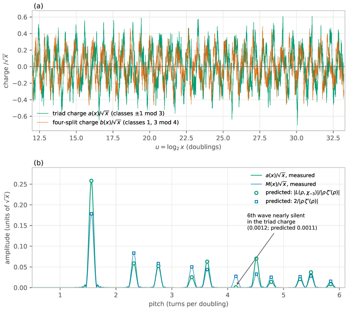
On the grid , , the amplitudes of , and at the pitches of the first twelve zeros agree with (6) to within (Table 3). The sixth zero has , and its wave is nearly silent in the triad charge: measured, predicted, against in M. The tenth zero has and its wave is nearly silent in the four-split charge: measured, predicted. At the twelve zeros the computed residuals and are of order , the precision of the zeros.
Table 3.
Wave amplitudes (units of ) of M, of the triad charge a and of the four-split charge b at the pitches (turns per doubling) of the first twelve zeros: measured from the counts to and predicted by (6). The last two columns are and .
Table 3.
Wave amplitudes (units of ) of M, of the triad charge a and of the four-split charge b at the pitches (turns per doubling) of the first twelve zeros: measured from the counts to and predicted by (6). The last two columns are and .
| pitch | M meas. | pred. | a meas. | pred. | b meas. | pred. | |||
|---|---|---|---|---|---|---|---|---|---|
Energies
The mean squares over the same grid, and over its two halves, agree with the sums (7) over the 2469 zeros with , completed by a tail beyond 3000 estimated from the mean of times the summand over and the density of the zeros (Table 4).
Table 4.
Mean square over in doublings, against the energies (7).
Table 4.
Mean square over in doublings, against the energies (7).
| measured | first half | second half | zeros | with tail | |
|---|---|---|---|---|---|
Figure 1.
(a) The triad charge (classes ) and the four-split charge (classes ) for , from the exact sieve. (b) Amplitude spectra in doublings of and , with the amplitudes (circles) and (squares) of (6) at the pitches of the zeros. The sixth wave is nearly silent in the triad charge.
Figure 1.
(a) The triad charge (classes ) and the four-split charge (classes ) for , from the exact sieve. (b) Amplitude spectra in doublings of and , with the amplitudes (circles) and (squares) of (6) at the pitches of the zeros. The sixth wave is nearly silent in the triad charge.
3. Prime Gaps with the Prime Squares
Proof of Theorem 4.
(i) Let be composite with no prime factor below p, and write with and . If then , which is excluded; so , the only prime in . If then , because by Bertrand’s postulate. Hence , which lies in the window since . Conversely every prime in and have no prime factor below p. (ii) An odd square is , and a square prime to 3 is . (iii) For integers , a gap leads from the class to the class , a gap from to , and a gap stays in its class. The crossings therefore alternate in direction, and the two counts differ by . By (ii) every prime square is . □
Corollary 1
(each square opens the next wheel). Let . On the gaps between consecutive members of the primes together with are the gaps of the wheel of integers prime to . The least composite member of this wheel is , and the next is .
For the window is and the wheel is that of 6: the numbers have gaps . For the window is and the wheel is that of 30; for it is and the wheel of 210. We have checked the window law directly through . The wheel of 30 is symmetric about 30, since : its members in lie at the distances 1, 7, 11, 13, 17, 19, 23, 29 from 30 on both sides, and , . With 49 inserted, the gaps from 7 to 67 are the gaps of the wheel of 30, namely , twice.
3.1. Gaps and Classes Up to 61
From 5 to 59 the gaps of the primes are
and with 25 and 49 inserted they are
Table 5 lists the ten triads up to 61. Without the squares the classes and hold 9 and 7 primes, and the four gaps of length 6 (, , , ) pass over 25, 35, 49 and 55: three times over the class and once over the class . With the squares inserted the two classes stand , each with exactly one composite not a square, and , and the two remaining gaps of length 6 pass over these two, one in each class. The gaps and number 5 and 5 without the squares and 7 and 7 with them.
Table 5.
The ten triads up to 61. The class holds nine primes and the composite 35; the class holds seven primes, the two squares 25 and 49, and the composite 55.
Table 5.
The ten triads up to 61. The class holds nine primes and the composite 35; the class holds seven primes, the two squares 25 and 49, and the composite 55.
| k | k | ||||||
|---|---|---|---|---|---|---|---|
| 1 | 5 | 6 | 7 | 6 | 36 | 37 | |
| 2 | 11 | 12 | 13 | 7 | 41 | 42 | 43 |
| 3 | 17 | 18 | 19 | 8 | 47 | 48 | |
| 4 | 23 | 24 | 9 | 53 | 54 | ||
| 5 | 29 | 30 | 31 | 10 | 59 | 60 | 61 |
3.2. Beyond 61
Up to the gaps between consecutive primes from 5 on number (), () and (). Table 6 compares the two classes with the prime squares counted at weight 0, 1 and . At weight 1 the class pulls ahead as the squares accumulate; at weight the difference stays within the oscillation carried by the zeros of , of scale , which is 543 at . Section 4 explains the weight .
Table 6.
The classes and of the primes up to x, the number of prime squares with (all in the class ), and for .
Table 6.
The classes and of the primes up to x, the number of prime squares with (all in the class ), and for .
| x | squares | difference | squares at weight 1 | squares at weight | ||
|---|---|---|---|---|---|---|
| 61 | 9 | 7 | 2 | 2 | 0 | 1 |
| 100 | 12 | 11 | 2 | 1 | 0 | |
| 86 | 80 | 9 | 6 | |||
| 616 | 611 | 23 | 5 | |||
| 63 | 22 | |||||
| 166 | 34 | |||||
| 444 | 189 | |||||
| 419 |
4. The Squares Carry the Lean
Proof of Theorem 5.
(i) For , . The finite product is entire and has no zeros in , because there. Likewise , with ; each has period , and W has divisors. (ii) , and J jumps by at each . Then , all sums being finite. (iii) By definition , the last sum is , and by the prime number theorem [21, Ch. 18]. The formula for J is Riemann’s [51], proved by von Mangoldt [62]. (iv) gives , so . (v) The left side is . Powers of 2 and 3 are not prime to 6. For , by Theorem 4(ii), so gives , and the terms total at most . □
Three Weights for One Square
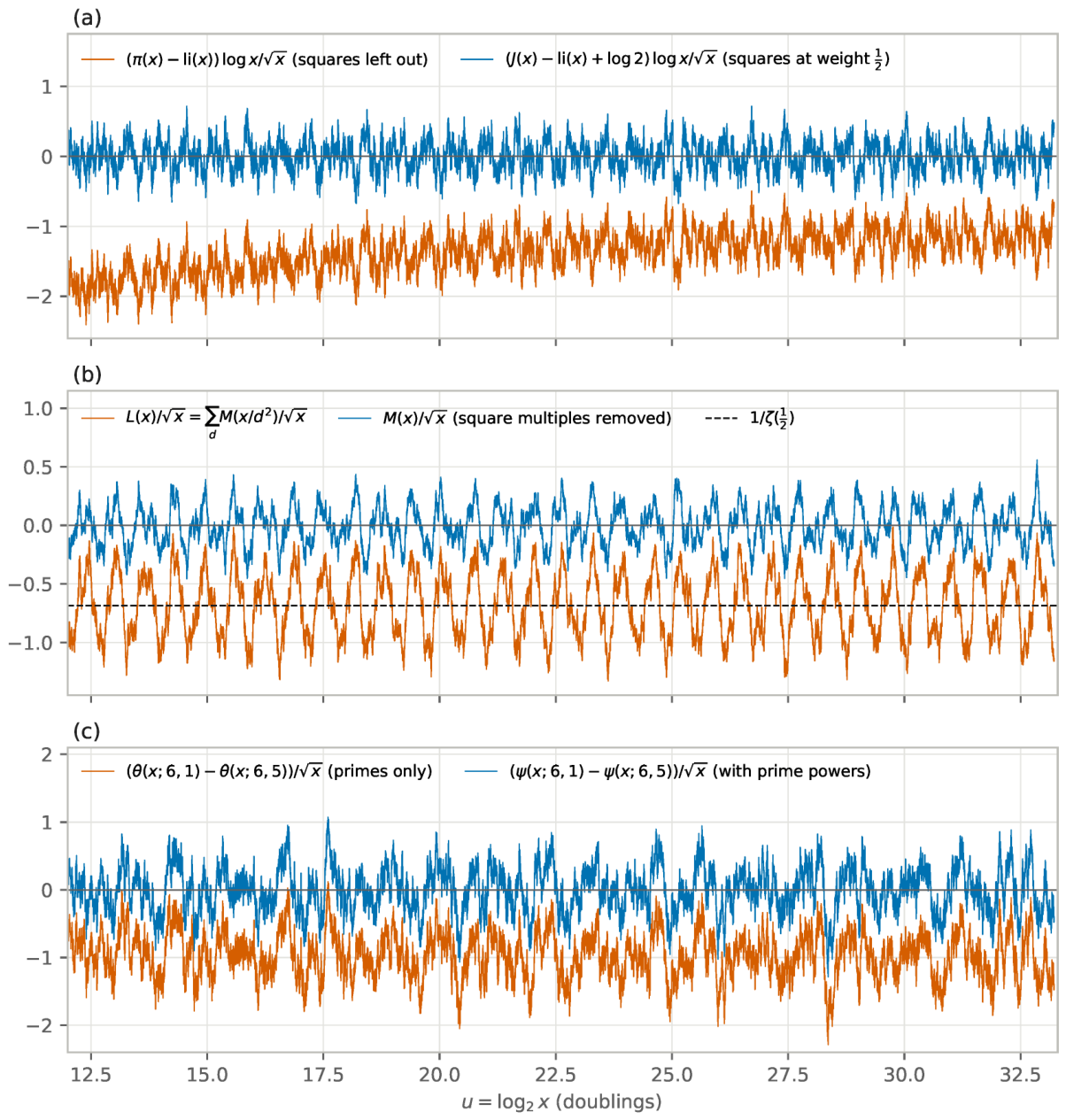
Since , the prime square sits on its own square-root horizon, and three counts weigh it differently. The wheel of modulus counts as a member, with weight 1 (Corollary 1); the primes leave it out, with weight 0; the logarithm of the Euler product counts it with weight (Theorem 5(ii)). By Theorem 5(i) every wheel series vanishes at every zero of , yet its count carries no wave: its error is bounded and periodic, and for the wheel of the spectrum in doublings of the error divided by has amplitude at most at every pitch in up to (Section 12). The zeros become waves only through the logarithm, which turns each of them into a pole of , and the count that carries these waves with no term of order is J, in which the squares have weight . By Theorem 5(iii), contains in addition : the lean of against li is the square term. In the same way carries the constant of the pole of at (Theorem 8(i)), and by Theorem 5(v) the difference carries , while is, by its explicit formula [21, Ch. 19], a sum of waves from the zeros of . This is the mechanism of Chebyshev’s bias identified by Rubinstein and Sarnak [53].
4.1. Measurements
The exact counts to (Section 12) give , li, M, L, and in the classes modulo 6 exactly. On the grid , ( points), Table 7 compares four counts with the squares left out and with the squares at weight .
Table 7.
The lean of four prime counts over : mean over the grid, fraction of the grid where the count is positive, and number of sign changes on the grid. In the prime power has weight , so its squares enter with weight relative to their position; .
Table 7.
The lean of four prime counts over : mean over the grid, fraction of the grid where the count is positive, and number of sign changes on the grid. In the prime power has weight , so its squares enter with weight relative to their position; .
| count | squares | mean | time above 0 | sign changes |
|---|---|---|---|---|
| left out | 0 | |||
| weight | 1816 | |||
| -multiples in | 0 | |||
| -multiples out | 826 | |||
| left out | 14 | |||
| weight | 1273 | |||
| left out | 0 | |||
| weight | 1408 |
The Balancing Weight
For , so that omits the squares and , the mean of over the grid is linear in w: it is at and at , and it vanishes at , with and on the two halves of the range. For the classes, the weight w that centres is ( and on the two halves).
The Waves are Unchanged
The amplitudes of at the first eight zeros are , , , , , , and , against , , , , , , and , and carries the same waves. The square weight moves the centre of the count and nothing else.
The Liouville Lean
has mean over the grid, against ; it holds almost the whole lean of L, while M itself is centred. Tanaka [57] found for , answering a question of Pólya [50]; in Table 7 the same count with its square multiples removed is M, which changes sign 826 times on the grid. Likewise at every grid point, although changes sign infinitely often [35], while changes sign 1816 times.
Figure 2.
The squares carry the lean, . (a) and . (b) and , with dashed. (c) and . In each panel the count with the squares at weight is centred and carries the same waves.
Figure 2.
The squares carry the lean, . (a) and . (b) and , with dashed. (c) and . In each panel the count with the squares at weight is centred and carries the same waves.
5. The Square-Root Horizon
We call the square-root horizon: it is the line where the squares series , and with it the part of carried by the prime squares and higher powers, stops converging. Write for , so that .
Proof of Theorem 6.
(i) For , , uniformly on compact sets, so S is analytic and is analytic and zero-free there. For , , and Möbius inversion, justified by absolute convergence, gives
For and , , so the second series converges to an analytic function of , which is S there. Since E has neither zeros nor poles in , is meromorphic there with the zeros of and their orders, and for . (ii) , so, with ,
an absolutely convergent series of terms . (iii) Since , (9) gives with . For and , and the bound of (i) makes R analytic in . Hence continues meromorphically to . The factor has no zeros or poles; has its only pole at and no zeros with [58, §3.3]. Since , has a simple zero at . For real , [58, §2.1], so , and . (iv) Let have multiplicity m. As , , tends to or to , and . So . By (iii), , while and stay bounded, because is analytic and zero-free at and ; hence as well. □
Remark 1
(the half-order zero is the square lean). The expansion of (9) is, term by term, Riemann’s expansion of Theorem 5(ii). The term , which near is , is the half-order zero of at the horizon, and in the count it is , the lean of π against li measured in Section 4. The half-order pole of E at is the same square term seen from the squares part.
Remark 2
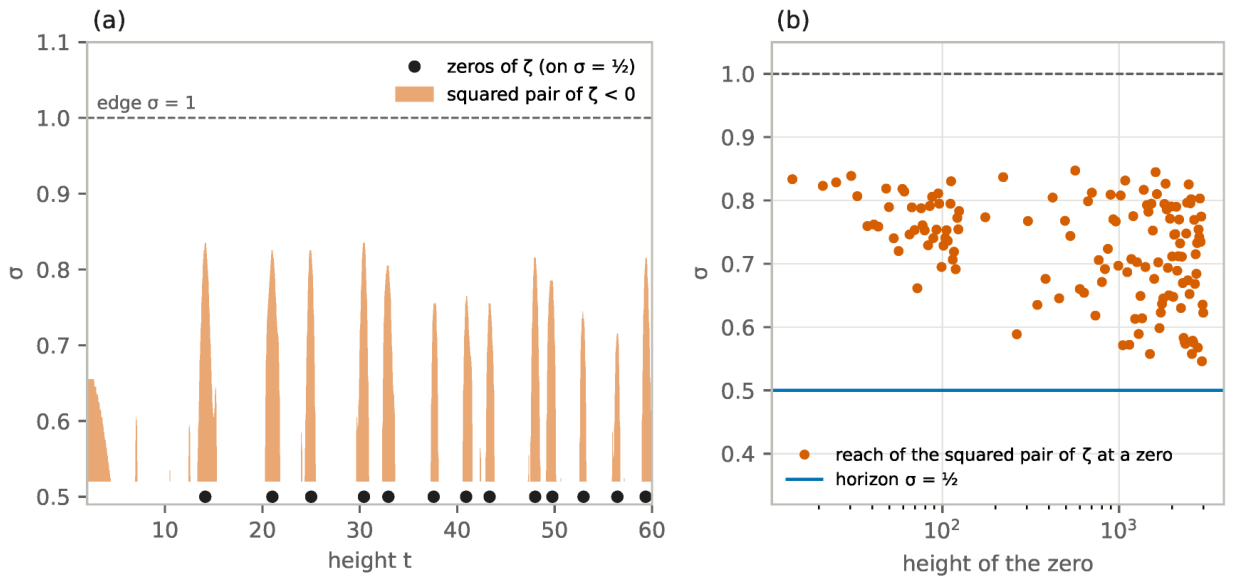
(edge and horizon). For ζ itself the squared pair is nonnegative for , [37], [58, §3.3], from the identity [58, (3.3.1)], which gives and, by the functional equation, . The inequality for ζ splits as : the prime part holds for , and the squares part holds all the way down to the horizon by Theorem 6(ii). The zeros of ζ in are exactly those of the prime factor F (Theorem 6(i)). At the horizon the squares part has a half-order pole and the prime factor a half-order zero, and by Theorem 6(iv) the squared pair of ζ and of F is negative arbitrarily close to the horizon at the height of every zero on it.
5.1. Measurements
The Squares Part
By (9), involves only in . At 200 random points with and the squared pair has minimum . Table 8 shows the half-order limits of Theorem 6(iii).
Table 8.
The half-order pole of the squares part E and the half-order zero of the prime factor at . The two limits add up to .
Table 8.
The half-order pole of the squares part E and the half-order zero of the prime factor at . The two limits add up to .
| limit | |||||||
|---|---|---|---|---|---|---|---|
The Reach of the Squared Pair of
For a zero let its reach be the largest at which . At the first 41 zeros and every 25th zero after them, 138 zeros in all up to height 3000, the reach lies between and (Table 9, Figure 3). For the prime factor alone the reach at the first twelve zeros is , , , , , , , , , , and . Above the reach the squared pair of is nonnegative at the sampled points of the window, and at such points has no zero; below it the band of negative values extends down to the zero on the horizon, as Theorem 6(iv) requires.
Table 9.
Reach of the negative band of the squared pair beside the zeros of .
| height of the zero | 50–100 | 100–300 | 300–1000 | 1000–2000 | 2000–3000 | |
|---|---|---|---|---|---|---|
| zeros | 10 | 19 | 15 | 21 | 35 | 38 |
| mean reach | ||||||
| largest reach |
Figure 3.
(a) The region , where the squared pair is negative, and the zeros of on . (b) The reach of the negative band at 138 zeros up to height 3000. The squares part satisfies everywhere above the horizon.
Figure 3.
(a) The region , where the squared pair is negative, and the zeros of on . (b) The reach of the negative band at 138 zeros up to height 3000. The squares part satisfies everywhere above the horizon.
6. The Prime Term at Every Height
By Theorem 6 every zero of in is a zero of the prime factor F, whose logarithm is the prime term for . At height t the prime term is the sum of the unit vectors weighted by , and its phases behave as independent in the sense of Theorem 7(i): any finitely many of them are jointly equidistributed.
Proof of Theorem 7(i)–(iii).
(i) By unique factorisation the numbers are linearly independent over : an integer relation gives , so every . Hence for every nonzero integer vector , and , and Weyl’s criterion [61] gives the equidistribution of modulo 1; this is Kronecker’s theorem in Weyl’s form [31, Ch. XXIII]. (ii) gives the variance. For the independent terms have mean 0 and summable variances, so the series converges almost surely [32], [23, Theorem 2.5.6]. For the real parts are independent, have mean 0, are bounded by 1 and have variances with divergent sum, so by Kolmogorov’s three-series theorem with truncation level 1 [23, Theorem 2.5.8] their sum does not converge almost surely; by Kolmogorov’s zero-one law it diverges almost surely. (iii) Let . Each factor has mean 1 and mean square , so by independence . For let , which is independent of and has mean 1; then . So converges in mean square, and . Also converges almost surely by (ii), so converges almost surely to , which is . □
Part (iv) consists of classical theorems: the mean square is Theorem 7.2 of [58], due to Hardy and Littlewood; is Theorem 9.15(A) of [58], due to Bohr and Landau [12]; the bound is Theorem 9.19(C) of [58], due to Selberg [54]; and the limiting distribution is due to Bohr and Jessen [10,11]. Since , the zeros with are a proportion of the zeros up to height T, for every fixed .
The squares series appears twice. In the model, the variance of the prime term is and the mean square of the Euler product is (Theorem 7(ii),(iii)); for itself, the mean square over heights is the same (Theorem 7(iv)). Both are finite exactly for . For the mean square has the second main term
where Matsumoto [36] proves for .
6.1. Measurements
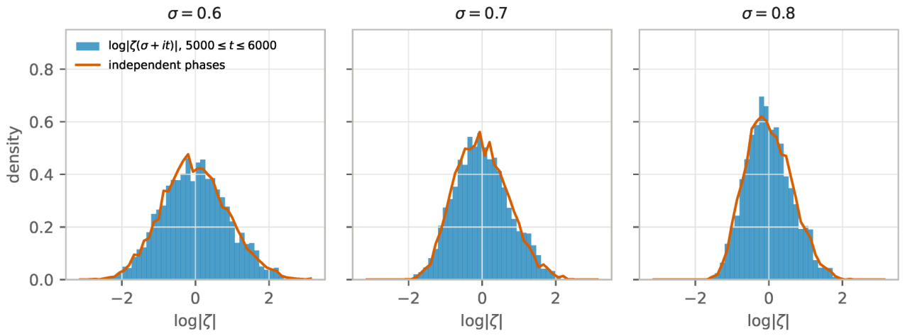
At 6000 heights drawn uniformly from we computed for . The model value is with the primes up to and independent uniform phases, plus a Gaussian term with the variance , , of the omitted primes; 6000 model values were drawn for each . Table 10 and Figure 4 compare the two.
Table 10.
The value distribution of at 6000 random heights in against the independent-phase model. The fourth column is the mean of over given by the two main terms of (10).
Table 10.
The value distribution of at 6000 random heights in against the independent-phase model. The fourth column is the mean of over given by the two main terms of (10).
| mean | by (10) | sd of | model sd | quantile | model | ||
|---|---|---|---|---|---|---|---|
The Deepest Dips
On the grid , , the least value of is (), at , between the close zeros and ; the model’s quantile at , one value per zero in the range, is and the least of model values, with the primes up to , is . At the least value is , at the same height, against and . The deepest dips off the line sit beside zeros on the line, and at every computed point is positive.
Figure 4.
Distribution of at 6000 random heights for (histograms), and of the independent-phase model (curves).
Figure 4.
Distribution of at 6000 random heights for (histograms), and of the independent-phase model (curves).
7. The Axiom of Harmonic Independence
Axiom 1
(harmonic independence). Harmonic independence is the absence of an integer relation. The prime waves are related only through a mechanism present in their construction. Because Unique Factorization guarantees that no integer relation exists between the primes, their wave frequencies are strictly linearly independent. A harmonic resonance between the primes beyond this explicit construction—such as a zero off the critical line—would be a relation without a mechanism.
The Waves and Their Frequencies
At height t the prime p enters the prime term as the wave , weighted by , of frequency in t; measured in doublings of p it is the clock of Section 11. An integer relation between the frequencies is a vector of integers, not all zero and finitely many nonzero, with , that is . Unique factorisation excludes every such vector. This is the first step of the proof of Theorem 7(i), and through Kronecker’s theorem in Weyl’s form it makes the phases of any finitely many primes jointly equidistributed on their torus: no finite set of prime waves holds a fixed phase relation over the heights, so the first part of the axiom is a theorem.
The Mechanism in the Construction
The waves are joined in by one mechanism, the Euler product , whose expansion into is unique factorisation itself. The squares part E and the prime factor F of Theorem 6 are this mechanism divided into its terms of order two and higher and its prime term. The relations among the waves measured in this paper are made by it: the lean carried by the squares at weight (Theorem 5), the variance of the prime term (Theorem 7(ii)), and the half-order zero of F at that matches the half-order pole of E (Theorem 6).
A Zero Off the Line
By Theorem 6(i) a zero with is a zero of the prime factor F. At the height it would be a relation among the prime waves weighted by , a resonance beyond the independence of their frequencies and beyond the relations that the Euler product supplies. The model in which the waves carry no relation at all, the independent phases of Theorem 7, has this form: there the random Euler product converges and is nonzero almost surely for every (Theorem 7(iii)). The axiom states as a principle that admits no relation among its prime waves beyond its construction; the theorems above give its first part, the linear independence of the frequencies, and with the axiom every zero of in the critical strip lies on the line .
8. The Forward and Reversed Terms at the Midpoint
The approximate functional equation of Hardy and Littlewood [27,28], in the form of Riemann and Siegel [58, §§4.12–4.16], [56], writes as a forward pattern, its reversal and a remainder:
Theorem 11
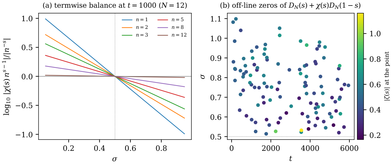
(termwise balance). Let with . For every , . This ratio is independent of n if and only if , where it equals 1. For it equals 1 for at most one real n, which is .
Proof.
. The functional equation gives and ; on , , so . For , is strictly monotone in n, and by Stirling’s formula [58, §4.12]. □
The Axiom at the Midpoint
On the critical line every forward term is balanced against its reversed partner, and off it no two pairs of terms are balanced at once. A zero of is a point at which the completed forward pattern and its reversal cancel. On the line the cancellation is between balanced partners; off it, it would require a relation among unbalanced terms that the construction (11) does not supply, which is what Axiom 1 excludes. The same structure is exact in a small graph, the medial antiprism: a stack of six triangles, each turned through against the next, in which every vertex is joined to every side midpoint of the neighbouring layer. Its lines form two strands, exchanged by the reversal of the vertical order. If the midpoint nodes are moved to the fraction f along their sides, lines of the two strands meet in each gap exactly three times at height f and three times at height , and only at the midpoint placement do all meetings lie on the middle plane.
A Mixed Construction
The Davenport–Heilbronn function , with the character modulo 5 with and , satisfies a functional equation of the same kind as that of and has zeros off the critical line [20], [58, §10.25]. It is the case that the axiom predicts. Its two Euler products are added with the relative weight , which equals the root number ; both have argument , so the mixing is forced by the functional equation. The logarithm of lives on the prime powers and gives every prime square the weight . The logarithm of f has nonzero coefficients at 130 of the 302 integers up to 400 that are not prime powers, beginning with , and its square weights are where is real and where . Its zero lies off the line. The zeros of f off the line are relations between prime waves that its construction supplies, which is what the axiom allows.
8.1. The Pair Without Its Remainder
The truncated pair , , satisfies , the functional equation of , so its zeros off the line come in pairs . Unlike , it has many. Scanning each range of constant N for (heights ), we located 116 zeros of with , each refined by Newton’s method to (Table 11, Figure 5). At every one of them the complete is far from zero: . The argument principle on a box of width and height about each of the 24 lowest finds no zero of off the line, and all zeros of in this range lie on the line [46]. At these heights the prime clocks are anti-aligned: the sum lies at median percentile among random heights nearby, and 33 of the 116 lie below the tenth percentile. The remainder closes every one of these meetings back onto the line.
Table 11.
Zeros of the truncated pair with located below height 6000, and the complete at them. Clock percentile: of among 2000 random heights within 200 of t.
Table 11.
Zeros of the truncated pair with located below height 6000, and the complete at them. Clock percentile: of among 2000 random heights within 200 of t.
| heights | zeros located | largest | least there | median clock percentile |
|---|---|---|---|---|
| 20 | ||||
| 27 | ||||
| 12 | ||||
| 19 | ||||
| 21 | ||||
| 17 |
Figure 5.
(a) The ratio at for several n: every pair of terms is balanced exactly at (Theorem 11). (b) The 116 located zeros of the truncated pair with , coloured by at the same point.
Figure 5.
(a) The ratio at for several n: every pair of terms is balanced exactly at (Theorem 11). (b) The 116 located zeros of the truncated pair with , coloured by at the same point.
8.2. Positive Chains
Following [24], define by , where , and the Jensen polynomials . Pólya proved that RH holds if and only if every is hyperbolic, that is, has only real roots [47]; Griffin, Ono, Rolen and Zagier proved hyperbolicity for every d and all sufficiently large n, and for and all n [24, Theorems 1, 2], the latter with a proof resting on a numerical check for ; an effective form of the first theorem is in [25]. For , is known to be hyperbolic for [16]. A real polynomial p has only real zeros if and only if the J-fraction of , produced by the Euclidean algorithm on p and , has positive couplings, and its zeros are moreover distinct if and only if the fraction has full length; then p is the characteristic polynomial of a Jacobi matrix with those positive off-diagonal entries [60, Theorem 43.1], [17, Ch. I]. RH is therefore the statement that every Jensen polynomial of is a chain with positive couplings, the chain ending early only at a repeated real zero. Positive coupling keeps the zeros real.
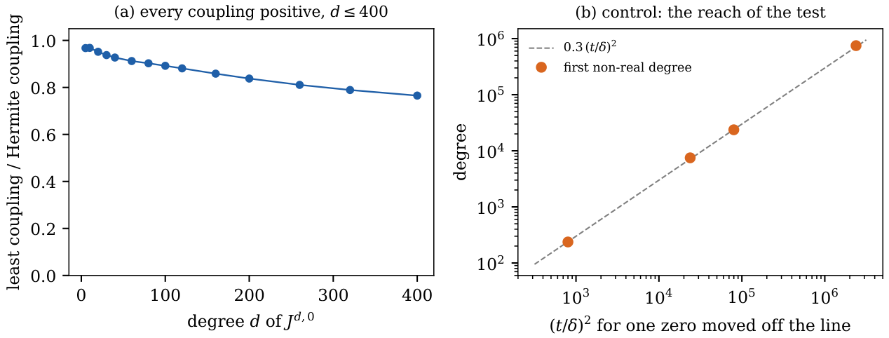
We computed for to 431 digits by Gauss–Legendre quadrature of Pólya’s kernel, checked against and , and ran the Euclidean algorithm in 420-digit arithmetic. These degrees are far below the range of [16] at ; what the chains add is the size of the couplings and a control of the reach. Every coupling is positive, at full length, for all 7029 polynomials with and in steps of 10, and for at . After scaling to unit mean square of the roots, the smallest coupling divided by the corresponding coupling of the Hermite chain, the limit of [24], is , at , (Figure 6a).
The test has a reach, which a control measures. In the product over the first 40 zeros, all Jensen polynomials up to degree are real-rooted. When one zero is moved off the line by , the first non-real degree is 237 for with , 23714 for with , 7499 for with and 749894 for with : about (Figure 6b). Degree 400 therefore certifies only , far less than the verification of [46], and by the same scaling the degree of [16] reaches of order . The chains are an exact form of RH, not a test of it at large heights.
Figure 6.
(a) The smallest coupling of the chain of , relative to the Hermite chain, for : all positive. (b) Control: the degree at which a single zero moved off the line by is first detected, against .
Figure 6.
(a) The smallest coupling of the chain of , relative to the Hermite chain, for : all positive. (b) Control: the degree at which a single zero moved off the line by is first detected, against .
9. The Reversed Pattern
Reversing the sign of every prime in the Euler product gives the reversed pattern . A zero of , where the forward pattern goes to in logarithm, is a pole of the reversed pattern, where it goes to : the same pattern read in reverse order.
Proof of Theorem 8.
(i) , so the product is and, being completely multiplicative with , equals for . If with then , so is finite and nonzero [58, §3.3] and is a pole of the same order. At , has a simple pole with residue and . (ii) The product is the identity [1, Theorem 2.19]. Hence counts the squares up to x. (iii) Let . For , , so ; the term is and the others total at most in absolute value, so and . Also [1, Ch. 4]. Since ,
and dominated convergence, with the bound , gives . Next, by (ii), so ; for , , which adds . This is (5) for , and letting gives the series. For both sides of (5) vanish in the limit. □
In the variable , with , (5) reads for every . The forward counterpart is , by (1) and [1]: the Möbius-weighted sawtooths rebuild the unit step, with its single jump at , and the Liouville-weighted sawtooths rebuild the square staircase, with a jump at every .
Centre and Lean
The forward pattern has a single pole, at its centre . The reversed pattern has its centre pole at , made by the squares through . In Perron’s formula for this pole contributes , and in that for , whose Dirichlet series is at , it contributes . The measured mean of is (Table 7), and leans to the positive side, while is centred (Table 12). The other poles of the reversed pattern are the zeros of . Every one computed lies on the vertical line through the centre : the 2469 below height 3000 used here, and all below height [46].
Forward Times Reversed at a Zero
The identity of Theorem 8(ii) holds as an identity of meromorphic functions. At a zero of its left side is a zero times a pole.
Proposition 1
(the identity at a zero). Let be a zero of ζ of order m with . Then:
- has a pole of order m at ρ;
- the product is analytic at ρ, with the value , which is finite and nonzero;
- for ,
In the squares pattern has a single pole, at the centre , where .
Proof.
Write with h analytic near and . Then , and the product of the two patterns is . This is analytic at because and, being nonzero, . Also by [58, §3.3]. For , . The only pole of is at 1, so the only pole of is at . □
At every zero, the zero of the forward pattern and the pole of the reversed pattern cancel in the product. They cancel in the same way whether or . For the point lies in . For it lies on the edge at height , away from the pole at 1. In both cases is finite and nonzero. The identity therefore holds at every zero and does not by itself tell a zero on the line from a zero off it. The pole of the squares pattern sits at the centre alone, and the centre is not a zero of . Table 13 gives the values at the first five zeros.
Table 13.
The identity of Theorem 8(ii) at the first five zeros, computed with 30 significant digits. The last column gives the difference between at and . At the same point the product differs from by at most ; both differences are of the size of the offset. With , the values give the edge weights of Section 10.
| residue, direct | |||
|---|---|---|---|
Checks
The identity (4) holds exactly at , 99, 100, 1000, 12345 and , with values 3, 9, 10, 31, 111 and 316. Table 14 shows the partial sums of (5); by (5) they equal , and the direct sums over agree with this to all digits shown. The exact sieve gives .
Table 14.
The Liouville-weighted sawtooths rebuild the square staircase: tends to .
| x | ||||
|---|---|---|---|---|
| 0 | ||||
| 1 | ||||
| 7 | ||||
| 9 | ||||
| 31 |
10. The Reversed Staircase Criterion
The criterion of Nyman and Beurling [9,41], in the form of Báez-Duarte [2], reads RH from the unit step , which the Möbius-weighted sawtooths rebuild exactly: RH holds if and only if . The reversed pattern rebuilds the square staircase (Theorem 8(iii)), and its alternating form f gives a second sawtooth criterion, built from the squares, in the direction that matters for RH: if then RH holds.
Lemma 1.
- (a)
- for .
- (b)
- (c)
- , and on an interval containing no multiple of k and no square in its interior, where with , the integrand integrates to . For the unit step, .
Proof. (a) Substituting gives [58, §2.1]. (c) Substitute ; then . □
Proof of Theorem 9.
(i) exactly on the intervals with n odd, so , and for , . By (5) at and at ,
since ; this is the stated identity, both series converging. The weights have the Dirichlet series .
(ii) Let attain , and . For , and , so and ; hence . Suppose with . By (i) and Lemma 1(a) the absolutely convergent Mellin integral of at is
The part over is , and by Cauchy–Schwarz the part over is at most . Hence . But , where and by the Euler product for . So for ; with for [58, §3.3] and the functional equation, every zero in the strip lies on .
(iii) Let . On , , and on , , so the Mellin integral of g converges absolutely on , and by (i) and Lemma 1(a) it equals , which is at a zero . For the unit step the transform of is . □
The Norm and the Value at
The Weight of a Zero
By the Mellin–Plancherel formula , and by Theorem 9(iii) no choice of coefficients moves the transform of the error at a zero on the line: it stays for the unit step and for the odd-square staircase. The reversed reading therefore weights each zero on the line by the value of on the edge at twice its height. For the unit step, Burnol [15] proved that the pinned values give , and Bettin, Conrey and Farmer [6] proved under RH and a hypothesis on , with
which is when every , the setting of [6]. The reversed pinned values attach to the zeros on the line the constant
computed over the 2469 zeros with and both signs of , completed by the tail beyond 3000 with the density of the zeros and the mean value of ; the ratio is . The edge weights of the first ten zeros are , , , , , , , , and .
10.1. Computation
For the Gram matrix is computed by exact integration on the intervals where both sawtooths are linear; for by Lemma 1(b), which agrees with the exact integrals to on the block. The inner products are computed by Lemma 1(c), splitting at the multiples of k and at the squares, with the tail beyond evaluated with the mean of ; the same procedure gives to within of , and direct quadrature on a truncated range agrees to . Then , with , by a Cholesky factorisation of G, whose condition number is at , at and at .
In double precision, with unit roundoff , the condition number bounds the relative error of the Cholesky solution by a quantity of order , far below the digits shown. A second implementation of the same formulas reproduces the condition number and the values of in Table 16 and Table 17 at the 15 values of N recomputed. The matrix serves only to compute at finite N. Theorem 9(ii) does not use it: the theorem holds for any coefficients that attain .
The Exact Weights Cut at N
The weights of Theorem 9(i) rebuild f at every point. They also satisfy , the value at of , where has its pole. This follows from Theorem 8(iii): , and . Cut at N, the weights give the error
For , with . So the part of over is , which tends to 0; this is the first step of the proof of Theorem 9(ii). The part over , where the sawtooths are not linear, is not controlled by . Table 15 computes both parts with the same Gram matrix, .
Table 15.
The odd-square staircase approximated by its exact weights cut at N, against the distance attained by the best coefficients. The error of the cut weights over is . Over it does not decrease.
Table 15.
The odd-square staircase approximated by its exact weights cut at N, against the distance attained by the best coefficients. The error of the cut weights over is . Over it does not decrease.
| N | , part over | part over | ||
|---|---|---|---|---|
| 10 | 0 | |||
| 30 | ||||
| 60 | 0 | |||
| 100 | 0 | |||
| 200 | ||||
| 300 | ||||
| 500 | ||||
| 700 | 0 | |||
| 1000 | ||||
| 1400 | 8 | |||
| 2000 | 18 |
Over the part over lies between and and does not decrease, while falls to . It is largest where the partial sum is largest: at and at . The exact weights cut at N rebuild f at every point but not in the norm. The vanishing of at the pole of settles the distance over . The distance over is carried by the coefficients that attain , which are chosen afresh at each N. By Theorem 9(ii) the statement gives RH, and it is a statement about those coefficients.
Table 16.
The distances of the odd-square staircase () and of the unit step () from the span of N sawtooths, for .
Table 16.
The distances of the odd-square staircase () and of the unit step () from the span of N sawtooths, for .
| N | 1 | 2 | 3 | 4 | 5 | 6 | 8 | 10 | 12 |
| N | 15 | 20 | 25 | 30 | 40 | 45 | 50 | 55 | 60 |
Table 17.
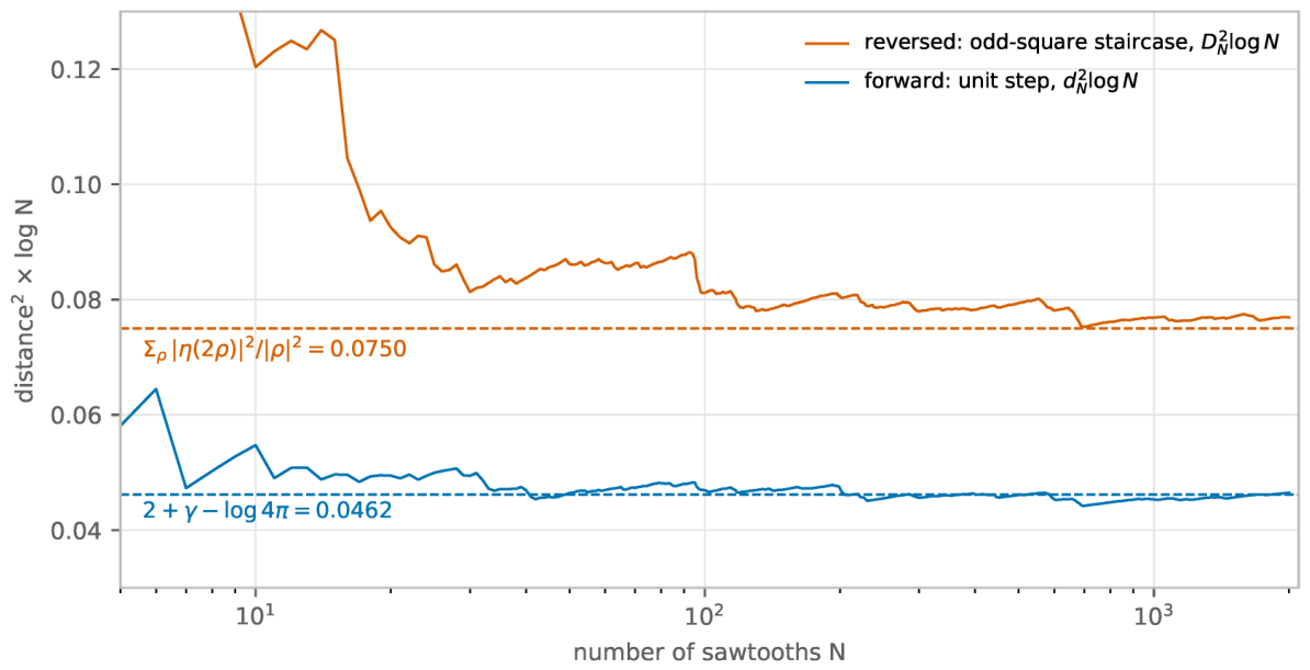
Distances times up to , against the constants and of the zeros. Over the means lie below and above ; the ratio at is , against .
Table 17.
Distances times up to , against the constants and of the zeros. Over the means lie below and above ; the ratio at is , against .
| N | ratio | window of N | mean | mean | ||
|---|---|---|---|---|---|---|
| 60 | 40–100 | |||||
| 100 | 100–300 | |||||
| 200 | 300–700 | |||||
| 300 | 700–1200 | |||||
| 400 | 1200–2000 | |||||
| 500 | ||||||
| 700 | constant | |||||
| 1000 | ||||||
| 1400 | ||||||
| 2000 |
Figure 7.
for the odd-square staircase and for the unit step, , computed from exact integrals, with the constants and of the zeros (dashed).
Figure 7.
for the odd-square staircase and for the unit step, , computed from exact integrals, with the constants and of the zeros (dashed).
11. Prime Clocks
The clock of a prime p is ; at height t it reads turns. At a whole turn the clock is aligned, ; at a half turn it is reversed, . At every clock is aligned and the Euler product has its pole at ; turning every clock by half a turn, , gives the reversed pattern of Section 9. The pitch in doublings of the wave of a zero (Section 2) is the reading of the clock of 2 at its height.
Proof of Theorem 10.
With these Fourier coefficients, the density of the readings of the clock of p over the zeros up to height T is
with at the alignment and at the reversal; this is the main term, each coefficient carrying an error . Every coefficient is negative: each prime pulls the zeros toward the reversal of its clock, with strength at . The zeros sit on the reversed side of every clock. For , and , and .
11.1. Measurements
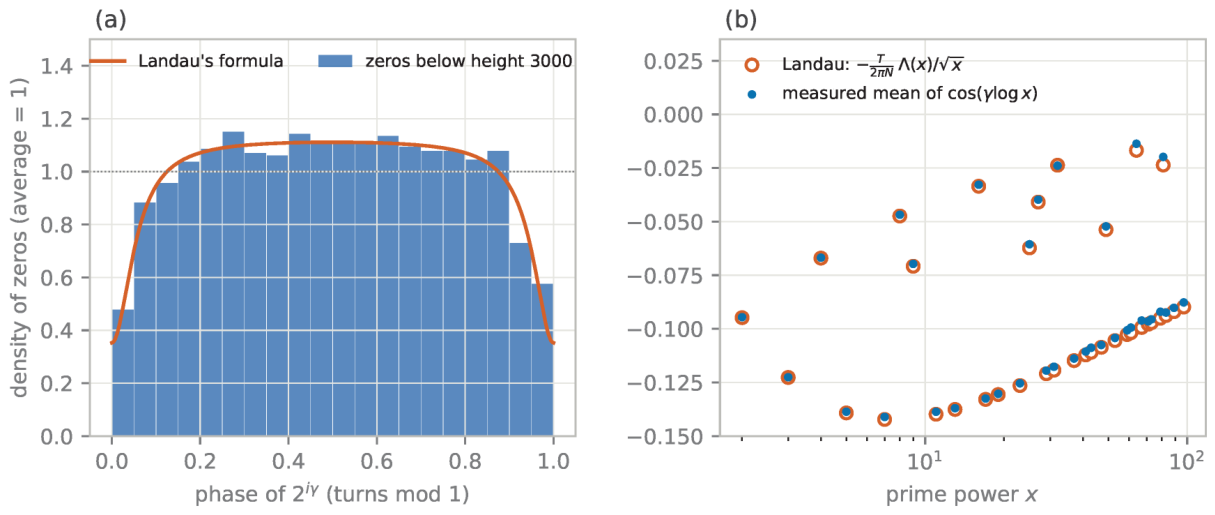
Over the 2469 zeros with , the mean of agrees with Landau’s formula to within at every prime power up to 13 (Table 18) and to within at all 35 prime powers up to 100, the largest difference being at . The density of the zeros on the clock of 2 follows (12) (Table 19, Figure 8): near the alignment it is and of the average, and elsewhere about .
Table 18.
Mean of over the 2469 zeros below height 3000, and .
| x | 2 | 3 | 4 | 5 | 7 | 8 | 9 | 11 | 13 |
|---|---|---|---|---|---|---|---|---|---|
| measured | |||||||||
| Landau |
Table 19.
Density of the zeros below height 3000 on the clock of 2, per tenth of a turn (average 1).
Table 19.
Density of the zeros below height 3000 on the clock of 2, per tenth of a turn (average 1).
| reading mod 1 | 0– | – | – | – | – | – | – | – | – | –1 |
|---|---|---|---|---|---|---|---|---|---|---|
| measured | ||||||||||
| by (12) |
Figure 8.
(a) Density of the 2469 zeros below height 3000 on the clock of 2, in twentieths of a turn, and the density (12). (b) Mean of over the same zeros at the 35 prime powers , and Landau’s formula.
Figure 8.
(a) Density of the 2469 zeros below height 3000 on the clock of 2, in twentieths of a turn, and the density (12). (b) Mean of over the same zeros at the 35 prime powers , and Landau’s formula.
The Clock of 2 in the Triad Charge
Since , the Euler factor of at 2 is , whose modulus at is : at a half turn of the clock of 2 and at a whole turn. The wave amplitudes of the triad charge in (6) carry , and over the zeros below height 3000 the mean of is for the 274 zeros within turn of a half turn and for the 130 zeros within turn of a whole turn; divided by the factor at 2, the two means are and . The sixth zero, whose wave is nearly silent in the triad charge (Table 3), reads turns, turn past a whole turn.
11.2. The Tenth Zero
The tenth zero reads turns on the clock of 2, within of , which in base two is ; there , and the clock is reversed. The reversed reading of Theorem 9(iii) weights the zero by
and at twice the height the clock of 2 reads turns, within of 11, which in base two is 1011: doubling the height moves the binary point one place, the half turn becomes a whole number of turns, and the factor of closes. For , , , and the weight is , against a mean of over the 2469 zeros.
The factor vanishes whenever the clock of 2 reads a half or a whole turn. of the 2469 zeros below height 3000, 71 have weight below : 49 lie within turn of a half turn and 22 within turn of a whole turn, more of them near the reversal, where the density (12) is higher. The first seven are, as (rank, , reading mod 1, weight), , , , , , and .
Remark 3
(rank and value). The silence of the tenth zero in the reversed reading is a property of its value, the height read on the clock of the prime 2, and not of its rank: the same clock silences 70 further zeros below height 3000. That prime is 2, written 10 in base two.
12. Methods of Computation
Counts to
An exact segmented sieve gives , and to and records , M, L, , , their restrictions to the classes 1 and , and in extended precision at checkpoints; it gives , and . The grid is interpolated linearly between checkpoints; J is formed from and a table of for .
The Tower
A second segmented sieve to computes for every n the values , and in integers and and in , stored as integer pairs for with , from the values at prime powers in Theorem 2. Each n is divided exactly by the primes up to , and the cofactor left after these divisions is 1 or a prime. All partial sums are exact and are recorded at checkpoints, which contain the grid, the points and the values , . The leaves come from these checkpoints for and from a table of , , for , and give every class of the tower at every level exactly.
Spectra and Energies
Mean over the grid removed, Hann window, direct evaluation of the Fourier sum at each pitch.
Zeros and Special Values
Squared Pair
on the grid , for Figure 3(a); the reach by 14 bisection steps in , with the minimum over 13 equally spaced heights in .
Value Distribution
at 6000 uniform random heights in ; the model as described in Section 6; the extremes on the grid .
Reversal
An exact sieve of to gives in double precision; (4) is checked by direct summation of L.
Sawtooth Integrals
As in Section 10; linear algebra in double precision by Cholesky factorisation. For the recomputation and Table 15, with , where is the harmonic number. The sum runs over , and the tail is evaluated with the mean of .
The Identity at a Zero
Gaps and Classes
A sieve of the primes to ; the window law is checked directly for .
Truncated Pair
evaluated in double precision with from the complex log-gamma function; for each N, the local minima of on the grid , , below a fifth of the median, refined by Newton’s method; at the points and on the boxes with mpmath at 15 digits [38]. The list of located zeros is not claimed to be complete.
Jensen Chains
from with Pólya’s kernel , by composite Gauss–Legendre quadrature on ; the Euclidean algorithm on the polynomial centred at the mean of its roots and scaled to unit mean square, in mpmath at 420 digits.
13. Concluding Remarks
The Triad Tower
The rebuild law splits by the residue of the divisor into the self-similar tower of Theorem 1: its zero classes repeat the whole law one level down, its unit classes are the character sums , carried only by the primes that the characters do not fix (Theorem 2), and its leaves are the values , whose energy is subpolynomially above x exactly when RH holds. At every zero of the triad of Dirichlet series is with (Theorem 3), and this fixes every wave of the tower: at the class values agree exactly with the leaves, and the twelve leading wave amplitudes of M, a and b and their energies agree with the zeros to within and .
The Squares
Each prime square opens the next wheel (Theorem 4): with 25 and 49 inserted, the primes to 61 are the wheels of 6 and 30, and the classes stand . All squares fall in the class , and the logarithm of the Euler product counts each of them with weight (Theorem 5). At that weight the lean of against li vanishes, with fitted weight , and the lean of the classes drops from to , with fitted weight ; the lean of L sits in its square multiples, and without them L becomes M, which is centred. The waves are unchanged.
The Horizon
The squares part E of is analytic, zero-free and satisfies the squared-pair inequality all the way down to the square-root horizon , where it has a half-order pole; the prime factor carries every zero of in and has at the matching half-order zero, which is the square lean of the prime count (Theorem 6, Remark 1). The phases are jointly equidistributed on every finite torus, and in the model with independent phases the prime term has the squares series as variance and converges almost surely exactly beyond the horizon (Theorem 7); for each fixed the zeros with form a proportion of those up to height T; and the values of at heights 5000 to 6000 follow the independent-phase law.
The Axiom
Harmonic independence is the absence of an integer relation (Axiom 1). By unique factorisation the frequencies of the prime waves admit none, which is a theorem (Section 7); the waves are related only through the Euler product that constructs , and a zero off the critical line would be a relation without a mechanism.
The Reversed Pattern
Reversing every prime turns into and every zero into a pole; forward times reversed is ; and the Liouville-weighted sawtooths rebuild the square staircase exactly (Theorem 8). The forward pattern has its single pole at its centre . The reversed pattern has its centre pole at , which gives its lean , and its other poles at the zeros of . In this form the Riemann Hypothesis is the statement that every pole of the reversed pattern lies on the vertical line through its centre. The results bear on this statement from four sides. The squares part is positive and zero-free down to that line (Theorem 6). In the independent-phase model of the prime factor, which carries the poles, the prime term converges almost surely beyond the line with the squares series as variance, and for each fixed the poles with form a proportion of those up to height T (Theorem 7). The odd-square staircase, rebuilt exactly by the reversed sawtooths, gives the criterion that puts every pole on the line, and computed to , stays within of the constant of the poles on the line over (Theorem 9, Table 17). Every prime clock pulls the poles toward its reversal as Landau’s formula prescribes, as verified over the 2469 poles below height 3000 at the 35 prime powers up to 100 and in the density on the clock of 2 (Theorem 10, Table 18 and Table 19). At each zero the forward zero and the reversed pole cancel in the product, leaving with residue . They cancel in the same way on the line and off it, so the identity holds at every zero and does not place it (Proposition 1). The exact weights of the staircase settle the distance over through the vanishing of at . Over they leave an error that does not decrease up to (Table 15), so the criterion rests on the coefficients that attain .
The Midpoint
The forward terms and their reversed partners are balanced, all at once, exactly on the critical line (Theorem 11). Without the remainder, the pair meets itself off the line: we locate 116 such zeros below height 5952, all at heights where the prime clocks are anti-aligned, and the complete is nonzero at every one of them. With the remainder, every zero computed lies on the line. As positive chains, the Jensen polynomials of are real-rooted wherever tested, and a control shows how far such a test reaches. In the reading of Axiom 1, a zero is a meeting of the completed pattern with its reversal, and the construction supplies balance at the midpoint only.
Outlook
The computations extend directly: the tower beyond by the rebuild law, the reversed distance beyond by Vasyunin’s closed form, and the densities of the zeros on the clocks of the odd primes by (12).
14. Data and Sources
External Inputs
All inputs are mathematical; no measured data are used.
- (i)
- All nontrivial zeros of with lie on the critical line [46].
- (ii)
- (iii)
- (iv)
- Classical and published theorems: the rebuild law [1, Ch. 3]; Littlewood’s criterion and the explicit formula for M [58, Theorems 14.25(C), 14.27]; Riemann’s formula for J [51,62]; the prime number theorem and the explicit formula for [21, Ch. 18, 19]; the Hurwitz zeta function, and [1]; Kronecker’s theorem and Weyl’s criterion [31,61]; the variance criterion and the three-series theorem [23,32]; the mean square of [58, Theorem 7.2] and its second term [36]; the density theorems of Bohr and Landau and of Selberg [12,54], [58, Theorems 9.15(A), 9.19(C)]; the value distribution [10,11]; Mertens’ inequality [37], [58, §3.3, (3.3.1)]; Chebyshev’s bias [53]; the sign changes of [35]; Pólya’s question [50]; the criterion of Nyman, Beurling and Báez-Duarte [2,9,41]; Vasyunin’s closed form [59]; Burnol’s bound [15]; the asymptotic of Bettin, Conrey and Farmer [6]; Landau’s formula [26,33]; the approximate functional equation [56], [58, §4.12]; the approximate functional equation [27,28]; zeros on the line and simple zeros [3,7,8,14,19,29,34,39,49,55]; the de Bruijn–Newman constant [22,40,48,52], [46, Corollary 2]; Jensen polynomials [16,24,25,47]; J-fractions and Favard’s theorem [17,60].
Computed Quantities
Every other number in the paper is computed from formulas stated in the text by the methods of Section 12: the tower and its waves and energies, the gaps and class counts, the leans and the fitted weights, the half-order limits and the reach of the squared pair, the value distribution and its extremes, the Liouville sums, the Gram matrices and the distances and , the error of the exact weights cut at N, the identity at the first zeros, the zeros of the truncated pair and the Jensen chains, the constants and , and the readings and densities of the zeros on the prime clocks.
References
- Apostol, T. M. Introduction to Analytic Number Theory. In Undergraduate Texts in Mathematics; Springer: New York, 1976. [Google Scholar]
- Báez-Duarte, L. A strengthening of the Nyman–Beurling criterion for the Riemann hypothesis. Atti Accad. Naz. Lincei Rend. Lincei Mat. Appl. 2003, 14, 5–11. [Google Scholar]
- Aryan, F. On an extension of the Landau–Gonek formula. J. Number Theory 2022, 233, 389–404. [Google Scholar] [CrossRef]
- Anthropic, Learning more about Claude’s mathematical capabilities. 10 August 2026. Available online: https://www.anthropic.com/news/riemann-zeta.
- Berndt, B. C. Ramanujan’s Notebooks, Part I; Springer: New York, 1985. [Google Scholar]
- Bettin, S.; Conrey, J. B.; Farmer, D. W. An optimal choice of Dirichlet polynomials for the Nyman–Beurling criterion. Proc. Steklov Inst. Math. 2013, 280, S30–S36. [Google Scholar] [CrossRef]
- Baluyot, S. A. C.; Goldston, D. A.; Suriajaya, A. I.; Turnage-Butterbaugh, C. L. An unconditional Montgomery theorem for pair correlation of zeros of the Riemann zeta-function. Acta Arith. 2024, 214, 357–376. [Google Scholar] [CrossRef]
- Baluyot, S. A. C.; Goldston, D. A.; Suriajaya, A. I.; Turnage-Butterbaugh, C. L. Pair correlation of zeros of the Riemann zeta function I: proportions of simple zeros and critical zeros. arXiv 2026, arXiv:2501.14545v3. [Google Scholar]
- Beurling, A. A closure problem related to the Riemann zeta-function. Proc. Nat. Acad. Sci. U.S.A. 1955, 41, 312–314. [Google Scholar] [CrossRef] [PubMed]
- Bohr, H.; Jessen, B. Über die Werteverteilung der Riemannschen Zetafunktion. Erste Mitt. Acta Math. 1930, 54, 1–35. [Google Scholar] [CrossRef]
- Bohr, H.; Jessen, B. Über die Werteverteilung der Riemannschen Zetafunktion. Zweite Mitt. Acta Math. 1932, 58, 1–55. [Google Scholar] [CrossRef]
- Bohr, H.; Landau, E. Ein Satz über Dirichletsche Reihen mit Anwendung auf die ζ-Funktion und die L-Funktionen. Rend. Circ. Mat. Palermo 1914, 37, 269–272. [Google Scholar] [CrossRef]
- Bombieri, E. Remarks on Weil’s quadratic functional in the theory of prime numbers, I. Atti Accad. Naz. Lincei Cl. Sci. Fis. Mat. Natur. Rend. Lincei (9) Mat. Appl. 2000, 11, 183–233. [Google Scholar]
- Bui, H. M.; Conrey, J. B.; Young, M. P. More than 41% of the zeros of the zeta function are on the critical line. Acta Arith. 2011, 150, 35–64. [Google Scholar] [CrossRef]
- Burnol, J.-F. A lower bound in an approximation problem involving the zeros of the Riemann zeta function. Adv. Math. 2002, 170, 56–70. [Google Scholar] [CrossRef]
- Chasse, M. Laguerre multiplier sequences and sector properties of entire functions. Complex Var. Elliptic Equ. 2013, 58, 875–885. [Google Scholar] [CrossRef]
- Chihara, T. S. An Introduction to Orthogonal Polynomials; Gordon and Breach: New York, 1978. [Google Scholar]
- Claude (Anthropic). More than two thirds of the zeros of the Riemann zeta function are simple and on the critical line, manuscript dated 11 August 2026. Available online: https://www-cdn.anthropic.com/95c246936988e43127bc6b2ceb7077c1dad2d68e.pdf.
- Conrey, J. B. More than two fifths of the zeros of the Riemann zeta function are on the critical line. J. Reine Angew. Math. 1989, 399, 1–26. [Google Scholar] [CrossRef]
- Davenport, H.; Heilbronn, H. On the zeros of certain Dirichlet series. J. Lond. Math. Soc. 1936, 11, 181–185 and 307–312. [Google Scholar] [CrossRef]
- Davenport, H. Multiplicative Number Theory, 3rd ed.; Montgomery, H. L., Ed.; Graduate Texts in Mathematics 74; Springer: New York, 2000. [Google Scholar]
- de Bruijn, N. G. The roots of trigonometric integrals. Duke Math. J. 1950, 17, 197–226. [Google Scholar] [CrossRef]
- Durrett, R. Probability: Theory and Examples, 5th ed.; Cambridge Series in Statistical and Probabilistic Mathematics 49; Cambridge University Press: Cambridge, 2019. [Google Scholar]
- Griffin, M.; Ono, K.; Rolen, L.; Zagier, D. Jensen polynomials for the Riemann zeta function and other sequences. Proc. Natl. Acad. Sci. USA 2019, 116, 11103–11110. [Google Scholar] [CrossRef] [PubMed]
- Griffin, M.; Ono, K.; Rolen, L.; Thorner, J.; Tripp, Z.; Wagner, I. Jensen polynomials for the Riemann xi-function. Adv. Math. 2022, 397, 108186. [Google Scholar] [CrossRef]
- Gonek, S. M. An explicit formula of Landau and its applications to the theory of the zeta-function. In A Tribute to Emil Grosswald: Number Theory and Related Analysis; Contemp. Math. 143, Amer. Math. Soc.: Providence, RI, 1993; pp. 395–413. [Google Scholar]
- Hardy, G. H.; Littlewood, J. E. The zeros of Riemann’s zeta-function on the critical line. Math. Z. 1921, 10, 283–317. [Google Scholar] [CrossRef]
- Hardy, G. H.; Littlewood, J. E. The approximate functional equation in the theory of the zeta-function, with applications to the divisor-problems of Dirichlet and Piltz. Proc. Lond. Math. Soc. 1923, 21, 39–74. [Google Scholar] [CrossRef]
- Hardy, G. H. Sur les zéros de la fonction ζ(s) de Riemann. C. R. Acad. Sci. Paris 1914, 158, 1012–1014. [Google Scholar]
- G. H. Hardy, Divergent Series; Clarendon Press: Oxford, 1949.
- Hardy, G. H.; Wright, E. M. An Introduction to the Theory of Numbers, 6th ed.; Heath-Brown, D. R., Silverman, J. H., Eds.; Oxford University Press: Oxford, 2008. [Google Scholar]
- Khintchine, A.; Kolmogoroff, A. Über Konvergenz von Reihen, deren Glieder durch den Zufall bestimmt werden. Mat. Sb. 1925, 32, 668–677. [Google Scholar]
- Landau, E. Über die Nullstellen der Zetafunktion. Math. Ann. 1912, 71, 548–564. [Google Scholar] [CrossRef]
- Levinson, N. More than one third of zeros of Riemann’s zeta-function are on σ = 1/2. Adv. Math. 1974, 13, 383–436. [Google Scholar]
- Littlewood, J. E. Sur la distribution des nombres premiers. C. R. Acad. Sci. Paris 1914, 158, 1869–1872. [Google Scholar]
- Matsumoto, K. The mean square of the Riemann zeta-function in the critical strip. Jpn. J. Math. (N.S.) 1989, 15, 1–13. [Google Scholar] [CrossRef]
- Mertens, F. Ueber eine Eigenschaft der Riemann’schen ζ-Function. Sitzungsber. Kais. Akad. Wiss. Wien. Math.-Naturwiss. Cl. 1898, 107, 1429–1434. [Google Scholar]
- The mpmath development team, mpmath: a Python library for arbitrary-precision floating-point arithmetic, version 1.3.0. 2023. Available online: https://mpmath.org/.
- Montgomery, H. L. The pair correlation of zeros of the zeta function. In Analytic Number Theory (St. Louis, 1972); Proc. Sympos. Pure Math. 24; American Mathematical Society: Providence, RI, 1973; pp. 181–193. [Google Scholar]
- Newman, C. M. Fourier transforms with only real zeros. Proc. Amer. Math. Soc. 1976, 61, 245–251. [Google Scholar] [CrossRef]
- Nyman, B. On Some Groups and Semigroups of Translations. Thesis, Uppsala, 1950. [Google Scholar]
- OEIS Foundation. Sequence A006880, number of primes < 10n, The On-Line Encyclopedia of Integer Sequences. Available online: https://oeis.org/A006880.
- OEIS Foundation. Sequence A084237, a(n) = M(10n), where M(n) is Mertens’s function, The On-Line Encyclopedia of Integer Sequences. Available online: https://oeis.org/A084237.
- OpenAI. The quasi-Riemann hypothesis: a zero-free half-plane Re(s) > 7/8, manuscript dated 30 September 2026, released 6 October 2026. Available online: https://github.com/openai/math/tree/main/preprints/The-Quasi-Riemann-Hypothesis-September-30-2026.
- OpenAI. The quasi-Riemann hypothesis, manuscript dated 5 October 2026, released 6 October 2026. Available online: https://github.com/openai/math/tree/main/preprints/The-Quasi-Riemann-Hypothesis-October-5-2026.
- Platt, D.; Trudgian, T. The Riemann hypothesis is true up to 3·1012. Bull. Lond. Math. Soc. 2021, 53, 792–797. [Google Scholar] [CrossRef]
- Pólya, G. Über die algebraisch-funktionentheoretischen Untersuchungen von J. L. W. V. Jensen. Kgl. Dan. Vid. Selsk. Math.-Fys. Medd. 1927, 7, 1–33. [Google Scholar]
- Polymath, D. H. J. Effective approximation of heat flow evolution of the Riemann ξ function, and a new upper bound for the de Bruijn–Newman constant. Res. Math. Sci. 2019, 6, 31. [Google Scholar] [CrossRef]
- Pratt, K.; Robles, N.; Zaharescu, A.; Zeindler, D. More than five-twelfths of the zeros of ζ are on the critical line. Res. Math. Sci. 2020, 7, 2. [Google Scholar] [CrossRef]
- Pólya, G. Verschiedene Bemerkungen zur Zahlentheorie. Jahresber. Deutsch. Math.-Verein. 1919, 28, 31–40. [Google Scholar]
- Riemann, B. Ueber die Anzahl der Primzahlen unter einer gegebenen Grösse. Monatsber. Königl. Preuss. Akad. Wiss. Berl. 1859, 671–680. [Google Scholar]
- Rodgers, B.; Tao, T. The De Bruijn–Newman constant is non-negative. Forum Math. Pi 2020, 8, e6. [Google Scholar] [CrossRef]
- Rubinstein, M.; Sarnak, P. Chebyshev’s bias. Exp. Math. 1994, 3, 173–197. [Google Scholar] [CrossRef]
- Selberg, A. Contributions to the theory of the Riemann zeta-function. Arch. Math. Naturvid. 1946, 48, 89–155. [Google Scholar]
- Selberg, A. On the zeros of Riemann’s zeta-function. Skr. Nor. Vid.-Akad. Oslo I 1942, 1–59. [Google Scholar]
- Siegel, C. L. Über Riemanns Nachlaß zur analytischen Zahlentheorie. Quellen und Studien zur Geschichte der Mathematik, Astronomie und Physik, Abt. B: Studien 1932, 2, 45–80. [Google Scholar]
- Tanaka, M. A numerical investigation on cumulative sum of the Liouville function. Tokyo J. Math. 1980, 3, 187–189. [Google Scholar] [CrossRef]
- Titchmarsh, E. C. The Theory of the Riemann Zeta-Function, 2nd ed.; Heath-Brown, D. R., Ed.; Oxford University Press: Oxford, 1986. [Google Scholar]
- Vasyunin, V. I. On a biorthogonal system associated with the Riemann hypothesis. St. Petersburg Math. J. 1996, 7, 405–419. [Google Scholar]
- Wall, H. S. Analytic Theory of Continued Fractions; Van Nostrand, New York, 1948. [Google Scholar]
- H. Weyl, Über die Gleichverteilung von Zahlen mod. Eins Math. Ann. 1916, 77, 313–352.
- H. von Mangoldt, Zu Riemanns Abhandlung “Ueber die Anzahl der Primzahlen unter einer gegebenen Grösse”. J. Reine Angew. Math. 1895, 114, 255–305. [CrossRef]
Table 12.
Value imbalance of the first K terms of the reversed and forward patterns. The reversed one leans around , the forward one around 0.
Table 12.
Value imbalance of the first K terms of the reversed and forward patterns. The reversed one leans around , the forward one around 0.
| K | |||||||
|---|---|---|---|---|---|---|---|
| (reversed) | |||||||
| (forward) |
Disclaimer/Publisher’s Note: The statements, opinions and data contained in all publications are solely those of the individual author(s) and contributor(s) and not of MDPI and/or the editor(s). MDPI and/or the editor(s) disclaim responsibility for any injury to people or property resulting from any ideas, methods, instructions or products referred to in the content. |
© 2026 by the authors. Licensee MDPI, Basel, Switzerland. This article is an open access article distributed under the terms and conditions of the Creative Commons Attribution (CC BY) license (http://creativecommons.org/licenses/by/4.0/).
Copyright: This open access article is published under a Creative Commons CC BY 4.0 license, which permit the free download, distribution, and reuse, provided that the author and preprint are cited in any reuse.