

Submitted:
04 October 2026
Posted:
07 October 2026
You are already at the latest version
Abstract
This study investigates exact algorithms for solving the Travelling Salesman Problem (TSP), formulated as the problem of finding a minimum Hamiltonian cycle in a complete weighted undirected graph. Two recursive algorithms are presented and analyzed. The first algorithm, denoted RecursiveHamiltonianCycle (RHC), performs an exhaustive recursive search of the solution space, while the second algorithm, denoted PrunedHamiltonianCycleSearch (PHCS), applies an early branch-pruning mechanism to eliminate non-promising partial solutions. The main objective of this research is to evaluate the influence of recursive branch pruning and initial upper-bound selection on the computational efficiency of exact TSP search procedures. A series of computational experiments was conducted using complete graphs containing between 12 and 21 vertices. The obtained results show that both algorithms always produce identical optimal Hamiltonian cycles. However, the PHCS algorithm requires significantly fewer recursive calls and substantially less execution time. Additional experiments demonstrate that the quality of the initial upper bound has a substantial impact on pruning efficiency. A nearest-neighbor heuristic was therefore used to generate high-quality initial solutions, resulting in further reductions in the search space. The results confirm that combining heuristic initialization with exact branch-pruning search significantly improves the practical applicability of exact TSP algorithms while preserving solution optimality.
Keywords:
travelling salesman problem
; exact algorithms
; recursive algorithms
; branch pruning
; near-est-neighbor heuristic
; combinatorial optimization
1. Introduction
An essential component of every software system is the set of algorithms used for data processing and for implementing the required functionality. Their characteristics determine both the amount of main memory required to store the data structures in use and the execution time of the computational processes. Therefore, when developing algorithms, it is important to achieve a balance between the computational resources utilized and the performance attained. Research in the fields of algorithms and data structures has been actively evolving for decades, and comprehensive results and fundamental concepts have been presented in [1,2,3,4]. When designing an algorithm to solve a specific practical problem, one of the first tasks is the selection of an appropriate data structure. The way in which data are modeled and processed has a direct impact on the organization of the computational process and on the choice of the algorithmic approach, which may be recursive or iterative.
The question of choosing between a recursive and an iterative approach in algorithm development has been the subject of numerous studies. Study [5] presents research on the preferences of novice and experienced programmers when designing and implementing algorithms. The obtained results indicate an increasing interest in the use of recursive solutions in recent years. Reference [6] emphasizes that the choice between a recursive and an iterative approach should be determined by the characteristics of the specific problem being solved. In [7], a method for transforming recursive algorithms into iterative ones through the use of incremental computation techniques is proposed. The reported experimental results show that, in many cases, iterative implementations require more memory but execute faster. Various approaches for optimizing memory usage in recursive algorithms are discussed in [8]. Approaches for transforming iterative processes into recursive implementations are presented in [9]. Recursive and iterative implementations of algorithms are widely applied in various fields of science and practice, with representative examples presented in [10,11,12]. Despite the considerable number of existing studies, the choice between recursion and iteration remains an important scientific and practical issue, particularly in the development of algorithms for solving complex combinatorial optimization problems.
One class of problems for which the choice of an appropriate algorithmic approach is of crucial importance is the class of problems modeled using graph structures. For such problems, the efficiency of the employed algorithms has a direct impact on the execution time and on the ability to solve practical problems with large input datasets. In the present study, the problem of finding a minimum Hamiltonian cycle in a weighted graph has been selected as a test problem. This problem is known in the literature as the Travelling Salesman Problem (TSP) [1]. The problem provides a suitable environment for the analysis and comparison of different algorithmic implementations, since it belongs to the class of NP-hard combinatorial optimization problems [2].
Graph theory is one of the most intensively studied areas of discrete mathematics and computer science. Over the last decades, it has found widespread application in the modeling and analysis of a variety of real-world systems and processes [13]. A graph is a mathematical structure consisting of two sets of elements: a set of vertices and a set of edges. Formally, a graph can be represented by the ordered pair of sets (Vertices, Edges), where Vertices = {vertex1, vertex2, ..., vertexk} is the set of vertices and Edges = {edge1, edge2, ..., edgep} is the set of edges. In directed graphs, each edge is represented by an ordered pair of vertices (vertexi, vertexj), whereas in undirected graphs the order of the vertices is irrelevant. If a numerical value is assigned to each edge through a weight function c(i, j), the graph is called weighted. If c(i, j) = c(j, i), the graph is an undirected weighted graph. A sequence of vertices vertex1, vertex2, ..., vertexq, in which every pair of consecutive vertices is connected by an edge, is called a path. A path whose starting and ending vertices coincide is called a cycle. A cycle that traverses each edge exactly once is called an Eulerian cycle, whereas a cycle that visits each vertex exactly once is called a Hamiltonian cycle. A graph is called complete if an edge exists between every pair of its vertices. Additional information on graph theory, graph data structures, and algorithms for solving various graph-related problems is presented in [13,14].
Graphs provide a convenient and effective framework for modeling, describing, and solving a wide range of practical problems. Numerous problems from science and practice, such as transportation problems, route planning problems, resource allocation problems, facility location problems, as well as problems related to timetable and schedule generation, can be successfully modeled using graph structures and solved with appropriate algorithms [13]. Some of these problems can be solved using linear optimization methods, whereas others require specialized algorithmic approaches. In many real-world applications, the size of the input data is considerable, which necessitates the use of efficient algorithms with acceptable execution times. In many cases, finding an exact solution requires a large number of computations, making the practical solution of the corresponding problem extremely difficult or even impossible within a reasonable amount of time [15]. For this reason, graph-based combinatorial optimization problems provide a suitable environment for the development, analysis, and comparison of algorithms with different characteristics in terms of accuracy and computational efficiency.
The number of real-world practical problems that can be modeled using graphs is extremely large. The present study considers the problem of finding a minimum Hamiltonian cycle in a complete, weighted, and undirected graph. This problem is a combinatorial optimization problem known in the literature as the Travelling Salesman Problem (TSP). A detailed description of the problem and its variants is presented in [16,17,18,19]. During the last decades, numerous algorithmic approaches for solving the TSP have been developed [20,21,22,23]. In general, these approaches can be divided into two main groups: exact and approximate methods. Exact algorithms guarantee the discovery of an optimal solution, but they are usually characterized by significant computational costs and are applicable mainly to problems of limited size [19,24,25,26]. On the other hand, approximate algorithms find a solution in a considerably shorter time, but they do not guarantee its optimality. The obtained solution may be close to the optimal one, but its quality depends on the approach used and on the characteristics of the particular problem [27,28,29]. In the present work, the TSP is used as a test environment for the analysis of two exact algorithms for finding a minimum Hamiltonian cycle. The first algorithm, denoted as RecursiveHamiltonianCycle (RHC), performs an exhaustive recursive search over the space of all possible solutions. The second algorithm, denoted as PrunedHamiltonianCycleSearch (PHCS), employs a mechanism for early pruning of non-promising branches in order to reduce the number of explored solutions. Through a comparative analysis of the two algorithms, the influence of the employed techniques on the efficiency of the computational process and the execution time is evaluated.
2. Materials and Methods
To evaluate the quality of solutions generated by approximation algorithms for a given problem, it is necessary to determine the optimal solution in advance, whenever this is practically feasible. For this purpose, two algorithms based on exhaustive exploration of the solution space have been implemented for the exact solution of the Travelling Salesman Problem (TSP). The first algorithm represents a modified version of a recursive approach presented in a previous study by the author [30], adapted for finding a minimum Hamiltonian cycle. The second algorithm employs a mechanism for the early pruning of non-promising branches in order to reduce the number of explored solutions. By analyzing the obtained results, it is possible to evaluate the influence of the selected algorithmic approach on the execution time of the computational process.
The two algorithms for the exact solution of the TSP operate on the set of vertices Vertices = {vertex1, vertex2, ..., vertexk} of the graph under consideration. Each permutation of these vertices defines a possible order for their traversal when constructing a Hamiltonian cycle. Since the number of all possible permutations of k elements is k!, the solution space grows factorially as the number of vertices increases. The generation of permutations is performed recursively. After fixing a vertex at position p, all possible arrangements of the remaining k−p vertices are generated. For each generated permutation, the length of the corresponding Hamiltonian cycle is calculated and the obtained solution is evaluated.
For the implementation of the two algorithms, several global data structures have been defined, including variables and dynamic arrays. These structures are used to store the current state of the computational process and are accessible from all functions of the software implementation. The list of these structures and their declarations is presented in Figure 1 (C++).
The variable indicator of type int is used as a counter for the recursive calls performed during the execution of the algorithms. The variable path_indicator, also of type int, stores the number of generated and evaluated Hamiltonian cycles. The variable improvements_indicator records the number of cases in which a Hamiltonian cycle with a shorter length than the best solution found so far has been identified. This variable is used by the optimized version of the algorithm, which applies a mechanism for the early pruning of non-promising branches. Under this approach, whenever the length of a partially constructed Hamiltonian cycle becomes greater than the length of the best cycle found so far, the further expansion of the corresponding solution is terminated. The reason is that adding new vertices and edges cannot lead to a shorter final cycle. In this way, the generation and evaluation of solutions that cannot improve the current optimum are avoided. The variable vertex_indicator of type int stores the number of vertices in the graph under consideration and is used during the traversal of all vertices. The length of the currently constructed Hamiltonian cycle is stored in the variable path_distance, whereas the length of the shortest cycle found so far is stored in the variable least_path_distance. Both variables are of type int.
The remaining globally declared structures are dynamic arrays. In these structures, memory for storing their elements is allocated during program execution, allowing their size to be determined dynamically according to the size of the problem under consideration. The dynamic array hamiltonian_path_array stores the indices of the vertices that form the currently constructed Hamiltonian cycle. Its size is vertex_indicator + 1, where the last element is equal to the first vertex of the cycle. In this way, the route is closed and a complete Hamiltonian cycle is formed. The dynamic array least_hamiltonian_path_array also has a size of vertex_indicator + 1 and stores the vertices of the shortest Hamiltonian cycle found so far. Traversing the vertices in the stored order produces a solution with the minimum length among all solutions considered up to that point. The dynamic array visited_vertices_array contains Boolean elements and is used to indicate whether a given vertex has already been visited within the current recursive branch. Its size is vertex_indicator + 1 and it is utilized by all implemented algorithms. The last dynamic structure, graph_weighted_matrix, represents the graph weight matrix. Each of its elements stores the length (weight) of the edge between the corresponding pair of vertices. If no edge exists between two vertices, a zero value is stored in the corresponding matrix cell. The dimensions of the matrix are vertex_indicator × vertex_indicator.
Figure 2 presents the implementation of the first algorithm for the exact solution of the Travelling Salesman Problem. The algorithm employs recursive depth-first search (DFS) with backtracking to generate all valid Hamiltonian cycles in the graph under consideration. Whenever a complete Hamiltonian cycle is generated, its length is calculated and compared with the length of the best solution found so far. To reduce the number of explored solutions, an optimization has been implemented that eliminates the generation of equivalent cycles obtained by traversing the same cycle in the opposite direction.
The algorithm uses a modification of the depth-first search (DFS) method. The RecursiveHamiltonianCycle function is called recursively on line 23. The process continues until all valid Hamiltonian cycles starting from the first vertex and passing through all remaining vertices of the graph have been generated. When the condition on line 4 is satisfied, the current Hamiltonian path is closed by returning to the starting vertex, thereby forming a complete Hamiltonian cycle. The length of the newly formed cycle is calculated on lines 6-9 by summing the weights of the corresponding edges. The obtained value is then compared with the length of the best solution found so far (line 10). If the current cycle is shorter, its length is stored in the variable least_path_distance, and the sequence of vertices is copied into the array least_hamiltonian_path_array (lines 11-16). If the vertex whose index is stored in pointer has already been visited within the current recursive branch, the execution of the function is terminated and backtracking is performed (line 18). Otherwise, the vertex is marked as visited using the array visited_vertices_array (line 19), after which all adjacent vertices that can participate in the continuation of the current Hamiltonian cycle are examined sequentially (lines 20-22). After the recursive call has finished, the vertex is marked as unvisited again (line 24). This technique allows all possible branches in the search tree to be explored and represents the fundamental mechanism of the backtracking method. The optimization of the algorithm is implemented on line 5. After incrementing the counter path_indicator, a check is performed to determine whether the number of generated cycles has reached the value stored in bound. This value is equal to the number of unique Hamiltonian cycles, since cycles obtained by traversing the same route in the opposite direction are equivalent and therefore are not considered repeatedly. In this way, the number of analyzed solutions is reduced by a factor of two without any loss of information regarding the optimal solution. The time complexity of the algorithm is factorial and is of the order of O((n−1)!/2), which represents a special case of exponential growth in computational complexity. The reason is that the algorithm performs an exhaustive generation and evaluation of all unique Hamiltonian cycles in the graph under consideration.
In this section, an optimized algorithm for the exact solution of the Travelling Salesman Problem is presented. Similar to the RecursiveHamiltonianCycle algorithm, it employs recursive depth-first search and backtracking to generate Hamiltonian cycles. The main difference lies in the pruning strategy applied during the construction of the solution. Whenever the current length of a partially constructed Hamiltonian cycle exceeds the length of the best cycle found so far, the further expansion of the corresponding branch is terminated. This allows a significant reduction in the number of explored solutions and, consequently, in the execution time. The implementation of the algorithm is presented in Figure 3.
Similar to the RecursiveHamiltonianCycle algorithm, this algorithm also employs recursive depth-first search (DFS) with backtracking. The function PrunedHamiltonianCycleSearch recursively calls itself on line 18. When the condition on lines 2–8 is satisfied, a complete Hamiltonian cycle has been constructed. In this case, the cycle length is stored in the variable least_path_distance (line 4), the counter improvements_indicator is incremented by one (line 5), and the vertices of the obtained solution are copied into the array least_hamiltonian_path_array (lines 6–8). During each recursive call, the weight of the newly added graph edge is added to the current length of the partially constructed cycle (path_distance) (line 16). A check is then performed to determine whether the obtained value is smaller than the length of the best solution found so far (line 17). Only if this condition is satisfied does the algorithm continue the recursive exploration of the corresponding branch (line 18). If the current length of the partially constructed cycle becomes greater than or equal to the value of least_path_distance, the execution of the corresponding branch is terminated. After returning from the recursive call, the last added edge is removed from the current solution by decreasing the value of path_distance (lines 19–20). In this way, a mechanism for the early pruning of non-promising solutions that cannot improve the current optimum is implemented. The effect of this optimization is a significant reduction in the number of explored states in the search tree. Nevertheless, the asymptotic worst-case time complexity of the algorithm remains factorial, of order O(n!), since under unfavorable input conditions it may still be necessary to consider almost all possible Hamiltonian cycles. In practice, however, the pruning mechanism substantially reduces the number of generated solutions and leads to a significant decrease in execution time.
Both exact algorithms for solving the TSP are initialized and executed through the InitializeRunExactAlgorithms function. This function prepares the required data structures, initializes the global variables, and invokes the selected algorithm. Its implementation is presented in Figure 4.
Memory allocation for the dynamic arrays used by the algorithms is performed on lines 2–4. On lines 5–8, the global variables and the auxiliary structures required for the execution of the computational process are initialized. The value of the variable bound is calculated on line 8 and determines the number of unique Hamiltonian cycles that can be generated by the RecursiveHamiltonianCycle algorithm without considering equivalent solutions obtained by traversing the same cycle in the opposite direction. The execution of a specific algorithm is performed by calling the corresponding function on line 9 or line 10. Depending on the selected experiment, one of the two function calls is enabled, while the other remains commented out. In this way, both algorithms use the same initialization process and can be compared under identical initial conditions.
The execution time of the two algorithms can be measured using the GetTickCount function. This function returns the number of milliseconds that have elapsed since the operating system was started. To determine the execution time, the function must be called immediately before and immediately after the execution of the algorithm under investigation, with the difference between the two values representing the duration of the computational process. Due to the multitasking nature of modern operating systems, the measured execution time may vary between different runs. To improve the accuracy of the experimental results, it is recommended that the algorithms be executed multiple times (for example, 10 times), after which the arithmetic mean of all measured execution times should be calculated.
3. Results
To evaluate the practical applicability of the proposed exact algorithms, a series of computational experiments was conducted using complete weighted undirected graphs containing between 12 and 21 vertices. The coordinates of all vertices were generated in a two-dimensional space, and the weight of each edge was defined as the Euclidean distance between the corresponding pair of vertices. The investigated graphs were complete graphs, meaning that every pair of vertices was connected by an edge. Consequently, for a graph containing n vertices, the number of edges m was equal to n(n–1)/2, while the degree d of each vertex was n–1. The graphs were constructed incrementally. Starting from graph G12, each subsequent graph was created by adding one additional vertex together with all edges connecting it to the existing vertices. In this way, graph Gn contained all vertices and edges of graph Gn–1. The number of unique Hamiltonian cycles in a complete undirected graph containing n vertices is given by (n–1)!/2. As a consequence, the size of the solution space grows factorially with increasing values of n. The rapid growth of the solution space demonstrates the computational difficulty of the Travelling Salesman Problem and motivates the search for optimization techniques capable of reducing the number of explored states. Table 1 summarizes the characteristics of the investigated graphs.
The first series of experiments was aimed at comparing the performance of the RecursiveHamiltonianCycle (RHC) algorithm and the PrunedHamiltonianCycleSearch (PHCS) algorithm. Both algorithms always produced identical optimal Hamiltonian cycles and identical objective values. Therefore, the comparison focuses exclusively on computational efficiency. The experiments were performed on a standard computer configuration with Win 11 Pro 64-bit operating system installed and the following hardware configuration: CPU: Intel® Core™ i7-4712MQ CPU @ 2.30 GHz 2.30 GHz; RAM: 8.00 GB.

Table 2.
Comparison between RHC and PHCS.
| Graph | Optimal Length |
RHC Recursions |
PHCS Recursions |
RHC Time |
PHCS Time |
| G_12 | 1320 | 596,778,072 | 701,001 | 14.9 s | 0.03 s |
| G_13 | 1388 | 7,812,368,010 | 1,986,732 | 194 s | 0.11 s |
| G_14 | 1461 | 110,024,183,594 | 12,656,921 | 45.9 min | 0.70 s |
| G_15 | 1512 | 1,658,826,162,812 | 89,960,671 | 11.5 h | 5.1 s |
| G_16 | 1568 | 26,663,480,363,520 | 276,274,409 | 7.7 days | 16.7 s |
The obtained results demonstrate that the pruning mechanism substantially reduces the number of recursive calls required to identify the optimal solution. For graph G16, the recursive exhaustive-search algorithm required more than seven days of execution time, whereas the optimized PHCS algorithm completed the search in approximately 17 seconds. As a result, a substantial improvement in performance was achieved. The effectiveness of the pruning mechanism increases with graph size, as longer partial paths are more likely to exceed the current best solution, leading to the earlier termination of non-promising branches. As illustrated in Figure 5, the gap between the numbers of recursive calls performed by the two algorithms widens considerably as the graph size increases.
Figure 5 confirms that both algorithms exhibit factorial growth in the number of recursive calls. However, the pruning mechanism significantly limits the expansion of the search tree, resulting in several orders of magnitude fewer recursive calls for the PHCS algorithm.
The experimental results for graph G17 revealed an important characteristic of the PHCS algorithm. Initially, the algorithm starts with a very large upper bound (MaxInt). During the search process, increasingly shorter Hamiltonian cycles are identified until the optimal solution is reached. To investigate the influence of the initial upper bound, the experiment was repeated using a high-quality Hamiltonian cycle as an initial reference solution.
Table 3.
Influence of the initial upper bound for graph G17.
| Variant | Recursions | Improvements | Time |
| PHCS | 1,745,599,627 | 53 | 144,953 ms |
| PHCS + good initial upper bound | 457,609,968 | 1 | 39,828 ms |
The optimal solution remained unchanged and had a length of 1681 px in both experiments. However, the number of recursive calls decreased by a factor of approximately 3.8, while the execution time decreased by a factor of approximately 3.6. These results indicate that the quality of the initial upper bound has a significant influence on the efficiency of the pruning strategy. Based on the observations obtained for graph G17, an additional optimization strategy was introduced. Before executing the PHCS algorithm, a nearest-neighbor heuristic was applied. The heuristic was executed once from each graph vertex, and the shortest Hamiltonian cycle obtained by the heuristic was selected as the initial upper bound for the exact search procedure. This initial solution does not guarantee optimality. However, it provides a relatively short Hamiltonian cycle, allowing the PHCS algorithm to eliminate a large number of non-promising branches at an early stage of the search process. The nearest-neighbor initialization strategy was applied to graphs G18-G21. The experimental results are summarized in Table 4. Path lengths reported in the columns NN Solution, Optimal Solution, and Difference are expressed in pixels.
The results demonstrate that the nearest-neighbor heuristic provides solutions that are very close to the optimum. For graph G18, the heuristic directly identified the optimal Hamiltonian cycle. For graphs G19-G21, the difference between the heuristic and optimal solutions remained relatively small, thereby enabling effective pruning during the exact search process.
Figure 6.
Comparison of nearest-neighbor and optimal solutions for graphs G18-G21.
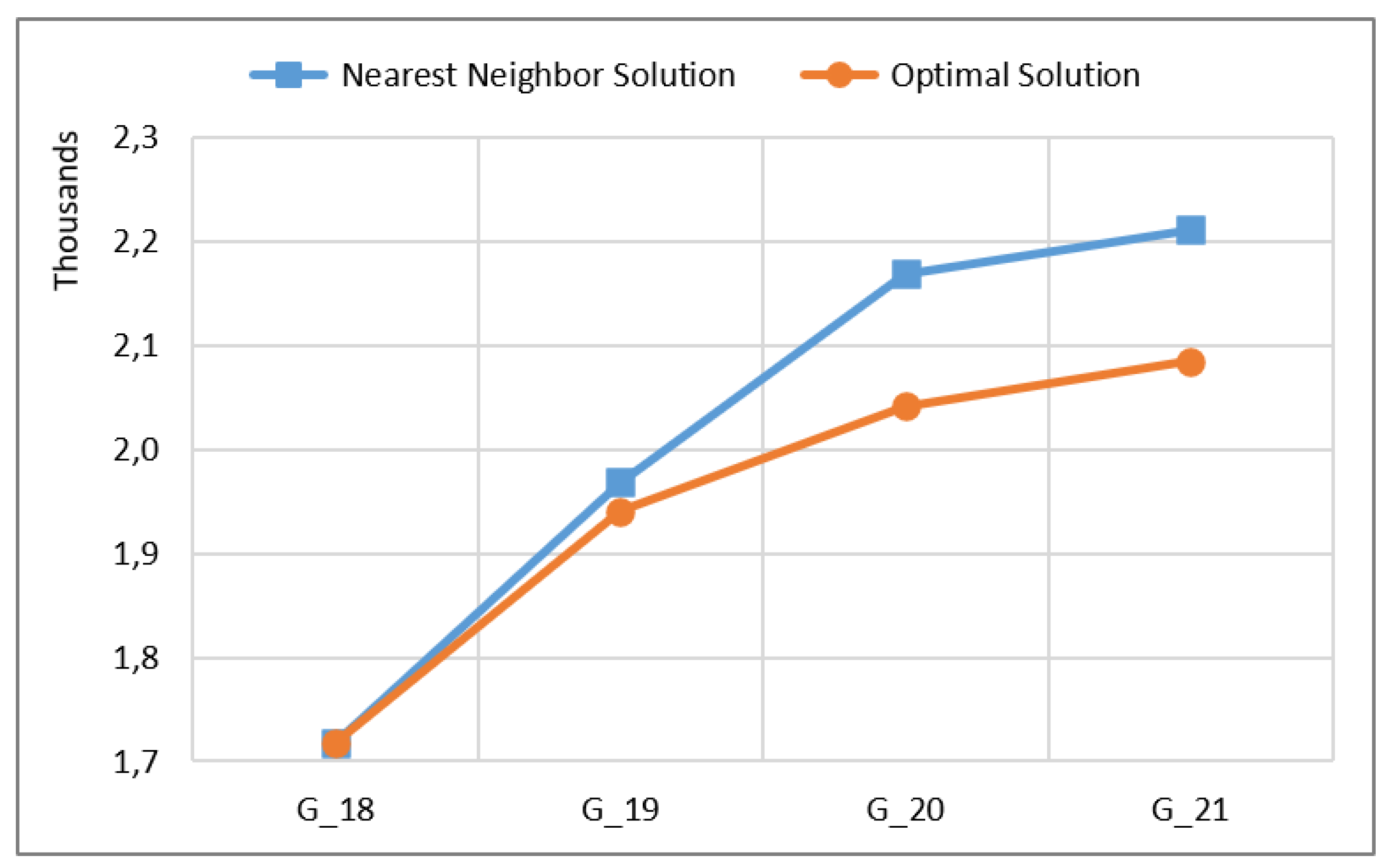
The experimental results demonstrate that all proposed optimization techniques contribute significantly to the practical performance of the exact TSP solver. The pruning mechanism implemented in PHCS dramatically reduces the number of recursive calls compared with exhaustive search while preserving the optimality of the obtained solution. In all investigated test instances, PHCS produced exactly the same optimal Hamiltonian cycle as RHC, confirming that the pruning strategy affects only the computational effort required to reach the solution and does not influence its correctness. Furthermore, the obtained results indicate that the effectiveness of pruning increases as the graph size grows. The difference between the numbers of recursive calls performed by the two algorithms becomes progressively larger for graphs containing more vertices, resulting in performance improvements of several orders of magnitude. The experiments also show that the quality of the initial upper bound has a direct impact on the effectiveness of the pruning process. A smaller upper bound leads to earlier elimination of non-promising branches and consequently reduces the number of recursive calls and the overall execution time. The results obtained for graph G17 clearly demonstrate that providing a high-quality initial solution considerably improves the efficiency of the exact search procedure.
Figure 7.
PHCS execution time for graphs G18-G21 (logarithmic scale).
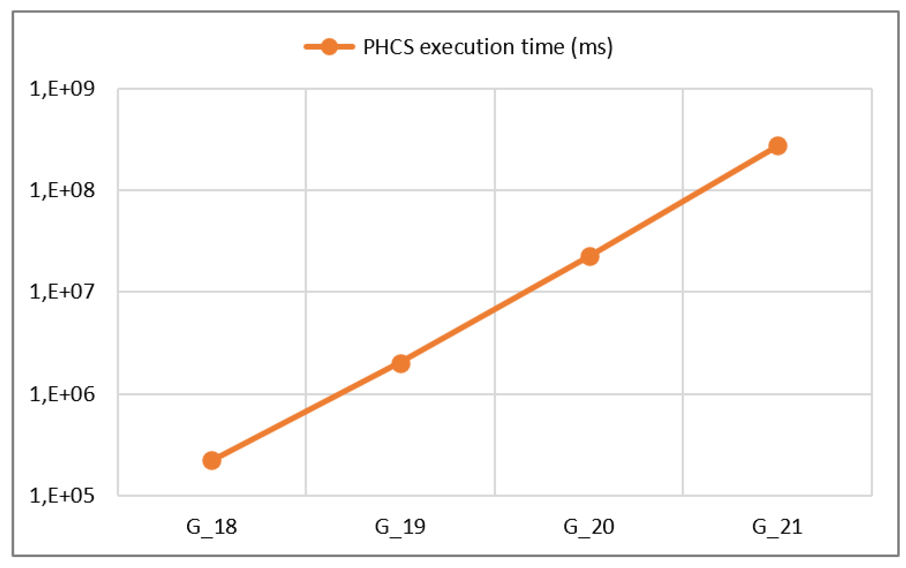
The nearest-neighbor heuristic proved to be an effective method for constructing such an initial upper bound. For graph G18, the heuristic directly identified the optimal Hamiltonian cycle, while for graphs G19-G21 the generated solutions remained very close to the optimal ones. As a result, only a small number of successive improvements was required before the exact algorithm reached the global optimum. This confirms that combining a fast heuristic procedure with an exact branch-pruning search can significantly improve the practical applicability of exact TSP algorithms. Despite all applied optimizations, the computational complexity of the exact solution process remains factorial. The execution time increased from approximately four minutes for graph G18 to more than seventy-six hours for graph G21. This behaviour reflects the combinatorial nature of the Travelling Salesman Problem and demonstrates that exact algorithms remain computationally demanding even when advanced pruning techniques and high-quality initial solutions are employed.
Overall, the conducted experiments show that the PHCS algorithm substantially outperforms exhaustive recursive search while maintaining exactness. The results further indicate that the use of a high-quality initial upper bound is one of the key factors affecting the efficiency of the search process. Although the proposed optimization techniques considerably extend the practical applicability of exact TSP algorithms, the rapid factorial growth of the solution space ultimately limits their use to medium-sized graph instances. Within the conducted experiments, graph G21 represented the largest problem instance for which an exact solution could still be obtained within a practically acceptable execution time.
4. Conclusions
The Travelling Salesman Problem is one of the best-known combinatorial optimization problems and is frequently used as a benchmark for evaluating exact and approximate optimization techniques. In the present study, two exact recursive algorithms for finding a minimum Hamiltonian cycle in a complete weighted undirected graph were investigated and compared. The first algorithm, RecursiveHamiltonianCycle (RHC), employs exhaustive recursive generation and evaluation of all unique Hamiltonian cycles. The second algorithm, PrunedHamiltonianCycleSearch (PHCS), introduces an early branch-pruning mechanism that terminates the exploration of partial solutions whenever their current length exceeds the length of the best solution found so far. The experimental results demonstrate that both algorithms always produce identical optimal solutions, confirming the correctness of the pruning strategy. A comparative analysis shows that the pruning mechanism dramatically reduces the number of recursive calls and the execution time required to obtain the optimal Hamiltonian cycle. For the investigated graph instances, the performance improvement increased with graph size, reaching several orders of magnitude.
An additional contribution of the study is the analysis of the influence of the initial upper bound used by the pruning mechanism. The experiments reveal that providing a high-quality initial solution significantly improves the efficiency of the exact search procedure. Based on this observation, a nearest-neighbor heuristic was used to construct an initial Hamiltonian cycle before executing the PHCS algorithm. The obtained heuristic solutions were found to be very close to the optimum and, in the case of graph G18, coincided with the optimal solution. This considerably increased the effectiveness of branch pruning and reduced the number of explored states. Despite all applied optimizations, the factorial growth of the search space remains the dominant limiting factor. The execution time increased from several minutes for graph G18 to more than seventy-six hours for graph G21, demonstrating that exact approaches to the TSP remain computationally demanding even when advanced pruning strategies are employed.
Author Contributions
Conceptualization, R.K. and V.K.; methodology, R.K.; software, R.K. and V.K.; formal analysis, R.K.; investigation, R.K.; data curation, V.K.; writing—original draft preparation, R.K. and V.K.; writing—review and editing, R.K.; visualization, V.K. All authors have read and agreed to the published version of the manuscript.
Data Availability Statement
The data involved in the paper are available upon reasonable request to the corresponding author.
Acknowledgments
The authors would like to thank the reviewers for their constructive comments.
Conflicts of Interest
The authors declare no conflict of interest.
Abbreviations
The following abbreviations are used in this manuscript:
| TSP | Travelling Salesman Problem |
| RHC | Recursive Hamiltonian Cycle |
| PHCS | Pruned Hamiltonian Cycle Search |
| DFS | Depth-First Search |
| NN | Nearest Neighbor |
| NP-hard | Nondeterministic Polynomial-time hard |
References
- Cormen, T.H.; Leiserson, C.E.; Rivest, R.L.; Stein, C. Introduction to Algorithms. In MIT Press; 2009. [Google Scholar]
- Sedgewick, R.; Wayne, K. Algorithms. In Pearson Education, 4th ed.; 2011. [Google Scholar]
- Skiena, S.S. The Algorithm Design Manual. In Springer, 2nd ed.; 2012. [Google Scholar]
- Knuth, D.E. The Art of Computer Programming. In Addison-Wesley; 2011; Vol. 3. [Google Scholar]
- McCauley, R.; Hanks, B.; Fitzgerald, S.; Murphy, L. Recursion vs. Iteration: An Empirical Study of Comprehension Revisited. In Proceedings of the 46th ACM Technical Symposium on Computer Science Education, 2015; pp. 350–355. [Google Scholar]
- Bhaskar, S. A Difference in Complexity Between Recursion and Tail Recursion. Theory Comput. Syst. 2017, 60(2), 299–313. [Google Scholar] [CrossRef]
- Liu, Y.A.; Stoller, S.D. From Recursion to Iteration: What Are the Optimizations? ACM SIGPLAN Not. 2000, 34(11), 73–82. [Google Scholar]
- Sundararajah, K.; Sakka, L.; Kulkarni, M. Locality Transformations for Nested Recursive Iteration Spaces. Proc. ACM SIGARCH Comput. Archit. News 2017, 45(1), 281–295. [Google Scholar] [CrossRef]
- Insa, D.; Silva, J. Automatic Transformation of Iterative Loops into Recursive Methods. Inf. Softw. Technol. 2015, 58, 95–109. [Google Scholar] [CrossRef]
- Musa, A.; Dubach, C. Automatic Recursion Elimination Using Recurrence Relations for Synthesis of Stack-Free Hardware. In Proceedings of the Asia and South Pacific Design Automation Conference (ASP-DAC), 2026; pp. 482–488. [Google Scholar] [CrossRef]
- Li, X.; Zhang, Q.; Wang, G.; Shi, Z.; Guan, Y. Reasoning About Iteration and Recursion Uniformly Based on Big-Step Semantics. Lect. Notes Comput. Sci. 2021, 13071, 61–80. [Google Scholar] [CrossRef]
- Leijen, D.; Lorenzen, A.F. Tail Recursion Modulo Context: An Equational Approach. J. Funct. Program. 2025, 35, e22. [Google Scholar] [CrossRef]
- Wilson, R.J. Introduction to Graph Theory. In Prentice Hall, 5th ed.; 2010. [Google Scholar]
- Benjamin, A.; Chartrand, G.; Zhang, P. The Fascinating World of Graph Theory. In Princeton University Press; 2017. [Google Scholar]
- Alekseev, V.E.; Boliac, R.; Korobitsyn, D.V.; Lozin, V.V. NP-hard Graph Problems and Boundary Classes of Graphs. Theor. Comput. Sci. 2007, 389(1-2), 219–236. [Google Scholar] [CrossRef]
- Alanzi, E.; Menai, M.E.B. Solving the Traveling Salesman Problem with Machine Learning: A Review of Recent Advances and Challenges. Artif. Intell. Rev. 2025, 58(9), 267. [Google Scholar] [CrossRef]
- Wang, Q.; Tang, C. Deep Reinforcement Learning for Transportation Network Combinatorial Optimization: A Survey. Knowl.-Based Syst. 2021, 233, 107526. [Google Scholar] [CrossRef]
- Cappart, Q.; Chételat, D.; Khalil, E.; Lodi, A.; Morris, C.; Veličković, P. Combinatorial Optimization and Reasoning with Graph Neural Networks. J. Mach. Learn. Res. 2023, 24, 1–61. [Google Scholar]
- Sciandra, L.; Esposito, R.; Grosso, A.; Sacerdote, L.; Zucca, C. Graph Convolutional Branch and Bound. Eur. J. Oper. Res. 2026, 334(3), 798–809. [Google Scholar] [CrossRef]
- Lyu, Z.; Islam, M.Z.; Yu, A.J. A Scalable and Adaptable Supervised Learning Approach for Solving the Traveling Salesman Problems. IEEE Trans. Intell. Transp. Syst. 2024, 25(11), 17092–17104. [Google Scholar] [CrossRef]
- Wang, S.; Rao, W.; Hong, Y. A Distance Matrix Based Algorithm for Solving the Traveling Salesman Problem. Oper. Res. 2020, 20(3), 1505–1542. [Google Scholar] [CrossRef]
- Liu, S.; Zhang, Y.; Tang, K.; Yao, X. How Good is Neural Combinatorial Optimization? A Systematic Evaluation on the Traveling Salesman Problem. IEEE Comput. Intell. Mag. 2023, 18(3), 14–28. [Google Scholar] [CrossRef]
- Perera, J.; Liu, S.H.; Mernik, M.; Črepinšek, M.; Ravber, M. A Graph Pointer Network-Based Multi-Objective Deep Reinforcement Learning Algorithm for Solving the Traveling Salesman Problem. Mathematics 2023, 11(2), 437. [Google Scholar] [CrossRef]
- Barbosa, L.H.; Uchoa, E. A Branch-Cut-and-Price Algorithm for the Traveling Salesperson Problem with Hotel Selection. Comput. Oper. Res. 2020, 123, 104986. [Google Scholar] [CrossRef]
- de Berg, M.; Bodlaender, H.L.; Kisfaludi-Bak, S.; Kolay, S. An ETH-Tight Exact Algorithm for Euclidean TSP. SIAM J. Comput. 2023, 52(3), 740–760. [Google Scholar] [CrossRef]
- Pereira, A.H.; Mateus, G.R.; Urrutia, S.A. Valid Inequalities and Branch-and-Cut Algorithm for the Pickup and Delivery Traveling Salesman Problem with Multiple Stacks. Eur. J. Oper. Res. 2022, 300(1), 207–220. [Google Scholar] [CrossRef]
- Kralev, V.; Kraleva, R. Combining Genetic Algorithm with Local Search Method in Solving Optimization Problems. Electronics 2024, 13(20), 4126. [Google Scholar] [CrossRef]
- Wei, B.; Xing, Y.; Xia, X.; Gui, L. A Novel Particle Swarm Optimization With Genetic Operator and Its Application to TSP. Int. J. Cogn. Inform. Nat. Intell. 2021, 15(4), A25. [Google Scholar] [CrossRef]
- Polnik, W.; Stobiecki, J.; Byrski, A.; Kisiel-Dorohinicki, M. Ant Colony Optimization-Evolutionary Hybrid Optimization with Translation of Problem Representation. Comput. Intell. 2021, 37(2), 931–963. [Google Scholar] [CrossRef]
- Kralev, V. An Analysis of a Recursive and an Iterative Algorithm for Generating Permutations Modified for Travelling Salesman Problem. Int. J. Adv. Sci. Eng. Inf. Technol. 2017, 7(5), 1685–1692. [Google Scholar] [CrossRef]
Figure 1.
Declarations of the global variables and dynamic arrays.
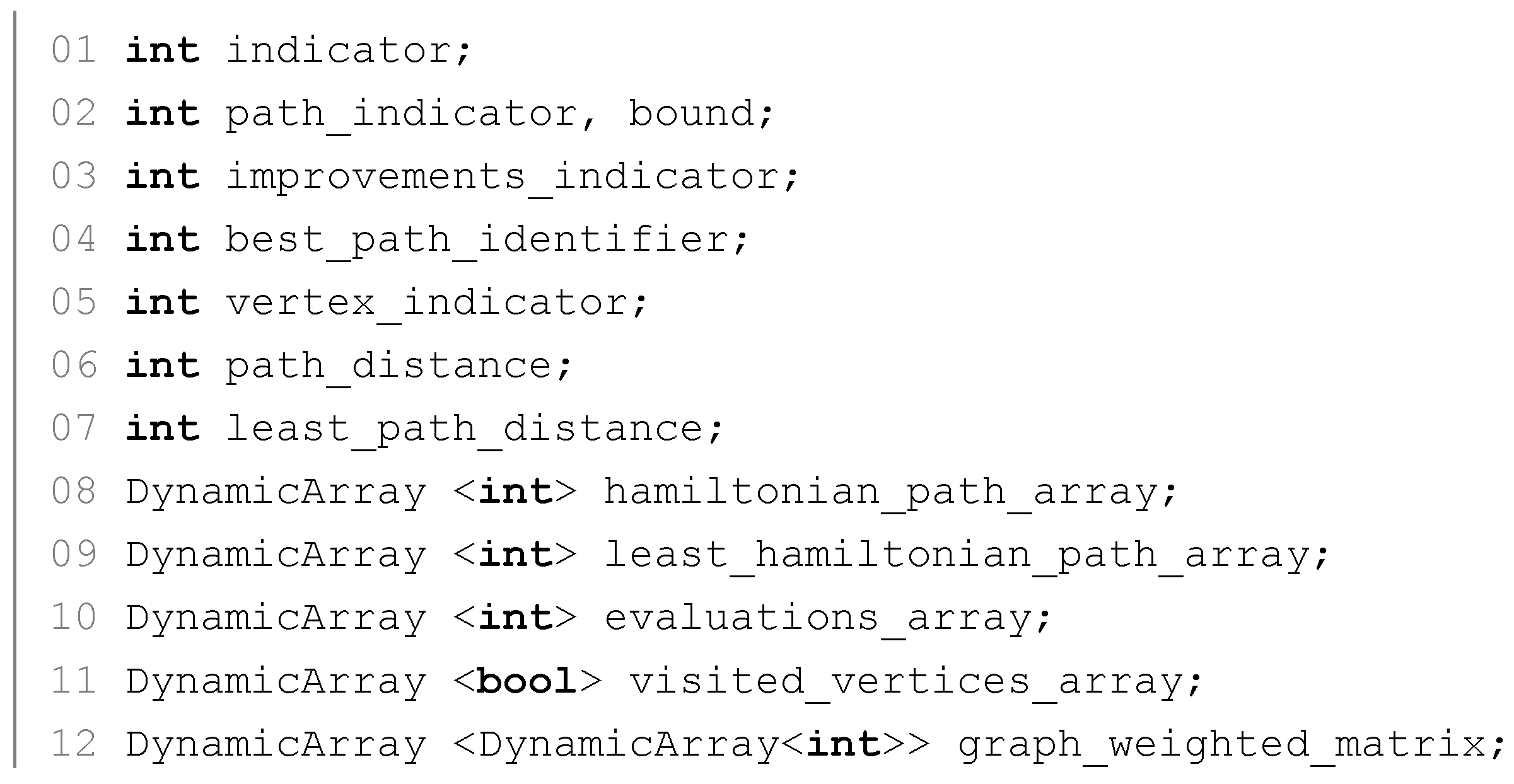
Figure 2.
Implementation of the recursive algorithm for the exact solution of the TSP (RecursiveHamiltonianCycle).
Figure 2.
Implementation of the recursive algorithm for the exact solution of the TSP (RecursiveHamiltonianCycle).

Figure 3.
Implementation of the optimized algorithm for the exact solution of the TSP (PrunedHamiltonianCycleSearch).
Figure 3.
Implementation of the optimized algorithm for the exact solution of the TSP (PrunedHamiltonianCycleSearch).
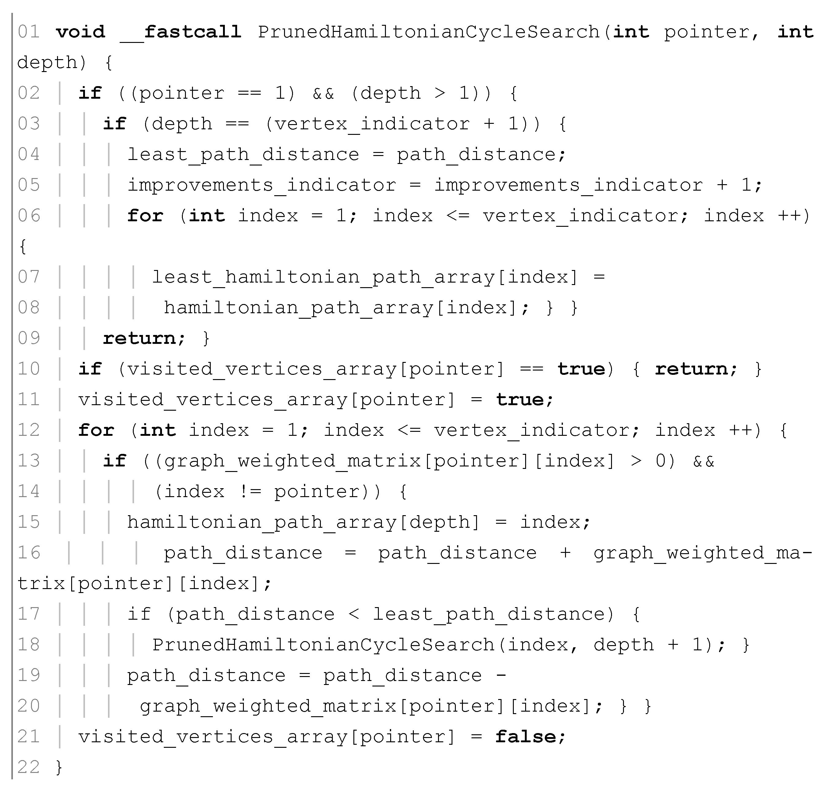
Figure 4.
Implementation of the initialization and execution function for the exact algorithms (InitializeRunExactAlgorithms).
Figure 4.
Implementation of the initialization and execution function for the exact algorithms (InitializeRunExactAlgorithms).
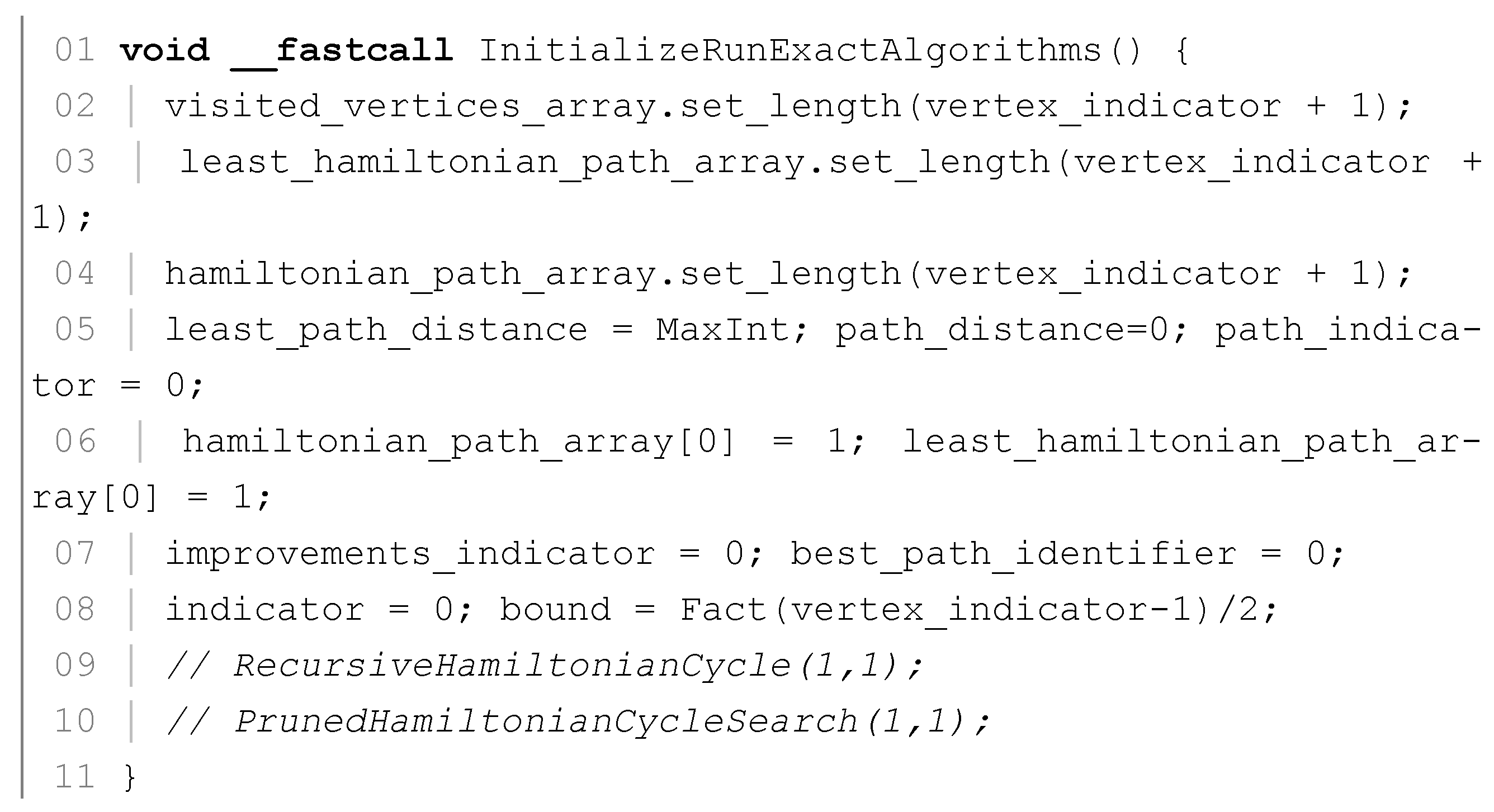
Figure 5.
Comparison of recursive calls performed by RHC and PHCS for graphs G12-G16 (logarithmic scale).
Figure 5.
Comparison of recursive calls performed by RHC and PHCS for graphs G12-G16 (logarithmic scale).
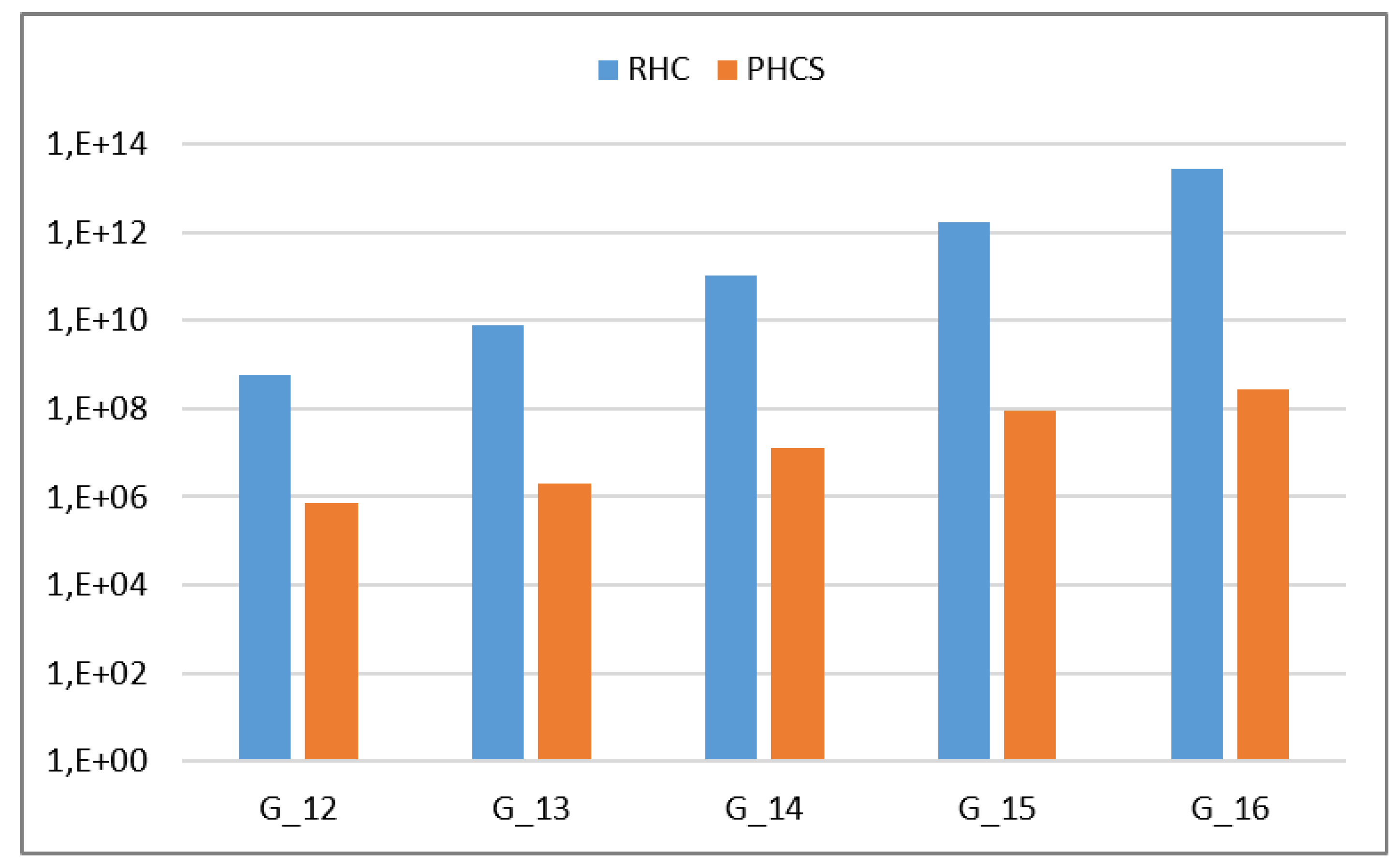
Table 1.
Characteristics of the investigated graphs.
| Graph | Vertices | Edges | Degree | Hamiltonian Cycles |
| G_12 | 12 | 66 | 11 | 19,958,400 |
| G_13 | 13 | 78 | 12 | 239,500,800 |
| G_14 | 14 | 91 | 13 | 3,113,510,400 |
| G_15 | 15 | 105 | 14 | 43,589,145,600 |
| G_16 | 16 | 120 | 15 | 653,837,184,000 |
| G_17 | 17 | 136 | 16 | 10,461,394,944,000 |
| G_18 | 18 | 153 | 17 | 177,843,714,048,000 |
| G_19 | 19 | 171 | 18 | 3,201,186,852,864,000 |
| G_20 | 20 | 190 | 19 | 60,822,550,204,416,000 |
| G_21 | 21 | 210 | 20 | 1,216,451,004,088,320,000 |
Table 4.
Results obtained using Nearest Neighbor initialization followed by PHCS.
| Graph | NN Solution | Optimal Solution | Difference | Improvements | Recursions | Time |
| G_18 | 1718 | 1718 | 0 | 1 | 2,437,686,589 | 223 s |
| G_19 | 1969 | 1941 | 28 | 2 | 20,668,648,235 | 1.47 h |
| G_20 | 2169 | 2042 | 127 | 5 | 219,361,653,648 | 18.1 h |
| G_21 | 2212 | 2085 | 127 | 4 | 2,542,401,565,780 | 76.4 h |
Disclaimer/Publisher’s Note: The statements, opinions and data contained in all publications are solely those of the individual author(s) and contributor(s) and not of MDPI and/or the editor(s). MDPI and/or the editor(s) disclaim responsibility for any injury to people or property resulting from any ideas, methods, instructions or products referred to in the content. |
© 2026 by the authors. Licensee MDPI, Basel, Switzerland. This article is an open access article distributed under the terms and conditions of the Creative Commons Attribution (CC BY) license (http://creativecommons.org/licenses/by/4.0/).
Copyright: This open access article is published under a Creative Commons CC BY 4.0 license, which permit the free download, distribution, and reuse, provided that the author and preprint are cited in any reuse.