

Submitted:
04 October 2026
Posted:
07 October 2026
You are already at the latest version
Abstract
Widely used open-source tools for map-based LiDAR localization of mobile robots are still largely organized by sensor suite: a 2D scanner typically calls for an AMCL-style particle filter over an occupancy grid, a 3D LiDAR for an NDT-based tracker over a point-cloud map, and an inertial- or GNSS-aided platform for a Kalman fusion node, often with different topics, parameters, initialization, and recovery behavior. Existing libraries already share one particle-filter core across 2D and 3D sensor models, and other systems already relocalize a robot by branch-and-bound scan matching. We describe PRISM-Loc, an open-source ROS 2 localization stack that places three established estimator families behind one node contract: laser2d, a likelihood-field Monte Carlo localizer; ndt3d, a planar NDT-MCL backend (Saarinen et al., 2013) that reuses the same particle filter with a Gaussian-voxel measurement model; and fusion3d, a 15-state error-state Kalman filter fusing LiDAR, IMU, and RTK-GNSS. Every backend publishes the same map→odom transform and pose with covariance and accepts the same /initialpose seeding, all filter mathematics live in Eigen-only C++17 cores that are tested without a ROS runtime, and laser2d relocalizes a kidnapped robot on request (at startup or by a service call) by deterministic branch-and-bound scan matching over a map-sized search window restricted to cells not marked occupied, keeping the top-K candidate poses and committing one only after several odometry-chained scans concentrate a normalized heuristic evidence score on it, and otherwise reporting the place as ambiguous. We claim no new estimator theory and no new verification principle; the contribution is this particular integration, released as software. In seeded closed-loop experiments on synthetic data that drive the actual cores, the 2D tracker holds a steady-state mean position error of 0.105 m, branch-and-bound relocalization succeeds on 97 of 100 kidnapped-robot queries in a 6 m room with zero false accepts at its default threshold, on 40 m and 80 m maps with repeated structure the single-scan rule accepts a wrong pose on 6 and 15 of 120 queries, which multi-scan verification reduces to 0 and 1 of 120 (pooled 95% Wilson interval 0.1–2.3%) while committing as many correct poses (242 against 241 of 300), and the ESKF bounds a 10 s aiding dropout to 0.125 m RMSE, although a 100-run NEES test shows that its covariance is overconfident (full-state NEES above the 95% interval at 89 of 120 epochs, mainly in attitude; bias blocks consistent). No external baseline and no real or public data are used, and no field-accuracy claim is made. Code: https://github.com/kjungmo/prism_loc.
Keywords:
mobile robots
; LiDAR localization
; Monte Carlo localization
; NDT
; error-state Kalman filter
; ROS 2
1. Introduction
Localizing a mobile robot against a prior map is, on paper, a solved problem, but the widely used open-source tools are still largely organized by sensor suite. A team fielding a 2D LiDAR typically reaches for nav2_amcl, a particle filter that tracks a planar pose against an occupancy grid and nothing else. A team with a 3D LiDAR may reach instead for an hdl_localization-style tracker built around 3D NDT registration (Koide et al., 2019). A team that must fuse inertial and satellite measurements may reach for a robot_localization-style node (Moore and Stouch, 2016), which composes an EKF over odometry, IMU, and GNSS but leaves the map-relative LiDAR measurement to another node. These tools differ in topic interface, parameter vocabulary, initialization, and recovery behavior, so a practitioner who moves from a 2D platform to a 3D one, or who adds a GNSS receiver, must re-integrate much of the localization layer.
The split is not universal, and several efforts reduce it. The survey of the ROS 2 navigation maintainers (Macenski et al., 2023) catalogs the shortcomings of AMCL and reports a proposed design for a localization framework that builds 2D and 3D localization systems from modular components. Beluga (Puga et al., 2024; Ekumen, Inc., 2022) is a ROS-agnostic C++17 Monte Carlo localization library whose ROS 2 nodes offer interface parity with nav2_amcl and pair one particle-filter core with likelihood-field and 2D and 3D NDT sensor models; Autoware’s pose-estimator arbiter (Autoware Foundation, 2024) launches several heterogeneous pose estimators and provides a mechanism to stop and resume them; and fuse (Locus Robotics, 2018) and MOLA (Blanco-Claraco, 2025) provide modular estimation frameworks. How a stack initializes, degrades, and recovers also matters in deployment: the Nav2 marathon deployment (Macenski et al., 2020) names low localization confidence as one of the two causes behind most of its recovery triggers. Classical MCL recovers from such failures through stochastic mechanisms, random particle injection or dual sampling (Fox et al., 1999; Thrun et al., 2001), which are hard to reproduce in a test; later systems add failure detection (Akai, 2023), keep several particle populations seeded by map matching (García et al., 2023), or reset a tracker from a branch-and-bound global search (Koide, 2021; Sasaki, 2026).
We describe PRISM-Loc, an engineering integration that packages three map-based LiDAR localization backends behind one ROS 2 node contract (Figure 1): laser2d, a 2D likelihood-field Monte Carlo localizer against an occupancy grid; ndt3d, a 3D NDT-MCL backend (Saarinen et al., 2013) that reuses the same particle filter with a voxel-Gaussian measurement model over a prior point cloud, sampling the planar pose; and fusion3d, a 15-state error-state Kalman filter (ESKF) that fuses 3D LiDAR, IMU, and RTK-GNSS with IMU-bias estimation. All three present the same interface, a map→odom transform, a pose with covariance on a private ~/pose topic that differs between the two nodes only by namespace and can be remapped (Table 2), and /initialpose seeding, so choosing between a 2D scan, a 3D cloud, and an inertial/GNSS-aided configuration is a launch-time choice of parameter or launch file rather than a change of interface. We claim no new estimator theory: likelihood-field MCL, NDT-MCL, ESKF fusion, and branch-and-bound scan matching are all established, and so are the broader patterns we use, namely one particle-filter core shared by 2D and 3D measurement models (Puga et al., 2024; Ekumen, Inc., 2022), branch-and-bound relocalization against a prior map (Koide, 2021; Hess et al., 2016), and tracking several global-localization hypotheses over time until the ambiguity is resolved (García et al., 2023; Gao et al., 2019). We are not aware of a released package that combines exactly the three backends below behind one contract with a relocalizer that can decline to commit; that combination is the contribution, delivered as usable open-source software. Table 1 lists the closest prior work for each component.
- One Pluggable Contract: three estimator families (2D likelihood-field MCL, 3D NDT-MCL, and LiDAR+IMU+RTK-GNSS ESKF fusion) present one ROS 2 map→odom contract, so the sensor suite selects a backend, not a stack with a different interface. Beluga already serves its likelihood-field and NDT particle filters through one node interface (Puga et al., 2024; Ekumen, Inc., 2022); the addition here is an inertial/GNSS Kalman backend that shares the same map→odom TF edge, pose message type, and /initialpose seeding (laser2d and ndt3d are chosen by one backend parameter, fusion3d by its own launch file); its covariance is overconfident in our test, so we release it as experimental (Section 5). The release adds fail-fast configuration checks, a startup watchdog that names the input that has gone silent, and a single-source parameter reference.
- Middleware-Free, Deterministic Cores: all filter mathematics sit behind an Eigen-only boundary with no rclcpp, tf2, or PCL, and all sampling routes through one seeded generator, so every algorithmic claim is exercised by 63 deterministic unit and integration tests and by closed-loop synthetic experiments that compile the cores directly. Middleware-independent estimator cores are established practice (Puga et al., 2024; Pedrosa, 2019); we list this as a property of the artifact, not as a research contribution.
- Global Relocalization That Can Abstain: for laser2d, the branch-and-bound correlative scan matcher of Hess et al. (2016), run over a max-pooled likelihood pyramid, finds candidate poses for a kidnapped robot from one scan and re-seeds the MCL particle set once a candidate is verified, in place of stochastic random-injection recovery. By the standard branch-and-bound argument of Hess et al. (2016), restated for our search set in Section 3.4, the search returns the best correlative score over the non-occupied (free or unknown) cells of the rotation–translation lattice; this is the discrete optimum of a surrogate score, not an optimal pose estimate. The search window is sized from the map, so the search is global up to a configurable compute cap (100 m per axis by default). Because the optimum of one scan can be a look-alike place, the node keeps the top-K distinct candidates, propagates each by odometry and re-scores it by a local branch-and-bound match, and commits one only when it holds most of a normalized heuristic evidence score over several scans, reporting the place as ambiguous otherwise. Tracking several hypotheses (García et al., 2023; Gao et al., 2019) and requiring evidence to persist over several scans and some motion before declaring a robot localized (Adurthi, 2023) are established, and concurrent work makes an abstaining decision explicit for LiDAR-to-BIM initialization (Zhang et al., 2026); what is specific here is this combination on 2D occupancy grids, wired to re-seed the shared MCL core.
We validate PRISM-Loc at the level of correctness and closed-loop behavior, not field accuracy. On seeded synthetic worlds generated to match the filters’ assumptions, the laser2d tracker holds a steady-state mean position error of 0.105 m while KLD-adaptive resampling shrinks the particle set from the 2000-particle ceiling to the 500-particle floor; branch-and-bound relocalization recovers 97 of 100 kidnapped-robot queries in a 6 m room under up to 80% beam clutter with zero false accepts at its default acceptance threshold, and on 40 m and 80 m maps recovers 50 and 41 of 60 poses that lie outside the fixed window of our first release, which recovered 2 and 0; there, however, a single scan accepts a wrong pose on 6 and 15 of 120 queries because repeated shelves look alike, and multi-scan verification brings this to 0 and 1 of 120 without losing correct fixes overall; and the ESKF limits a 10 s loss of all aiding to 0.125 m position RMSE, while a 100-run Monte Carlo NEES test shows that its covariance is overconfident, mainly in attitude. These numbers demonstrate that the assembled pipelines behave as intended; they are not a benchmark. We run no external baseline and use no real or public data, so we make no claim of accuracy or robustness relative to nav2_amcl, Beluga, MH-AMCL, or the global-localization methods of Section 2; that comparison is planned (Section 5).
2. Related Work
Monte Carlo Localization. Particle-filter localization was introduced by Dellaert et al. (1999) and Fox et al. (1999), who represent the pose posterior as a weighted sample set updated by motion-model prediction, sensor-likelihood weighting, and resampling, and who demonstrated global localization from a uniform prior on real robots. Thrun et al. (2001) later hardened MCL against accurate sensors and the kidnapped-robot problem via Mixture-MCL’s dual sampler, and Fox (2003) made the sample size adaptive through KLD-sampling; the odometry motion model and likelihood-field sensor model we use are the textbook forms of Thrun et al. (2005). The particle-filter core of PRISM-Loc is a direct descendant of this line and of its nav2_amcl lineage; we contribute no new filter theory. Sharing one such core across measurement models is not new either. Beluga (Puga et al., 2024; Ekumen, Inc., 2022) is a ROS-agnostic, extensible C++17 MCL library; its ROS 2 nodes offer interface parity with nav2_amcl and combine one particle-filter core with likelihood-field, beam, and 2D and 3D NDT sensor models, and its 3D NDT node estimates a full pose, which is more general than the planar state of our ndt3d backend. Earlier, mcl_3dl (Watanabe, 2016) implemented 3D/6-DoF point-cloud MCL against a reference cloud for ROS, and Martín Rico et al. (2023) replace Nav2’s AMCL with an MCL over Gridmaps and Octomaps for non-planar terrain. Other work makes MCL recovery more reliable: Akai (2023) estimates the reliability of the MCL estimate to detect failure and integrates a global localization method through importance sampling for quick re-localization, and MH-AMCL (García et al., 2023) maintains several particle populations, created by multi-scale map matching, and outputs the most reliable one. PRISM-Loc instead delegates recovery to a deterministic branch-and-bound search (Section 3.4) followed by multi-scan verification (Section 3.5).
NDT Representations and Measurement Models.Biber and Straßer (2003) introduced the Normal Distributions Transform, modeling a scan as per-cell Gaussians and reducing registration to Newton optimization of a smooth score; Magnusson et al. (2007) generalized the representation to 3D voxel grids for field deployment on mining vehicles. Both use NDT for deterministic scan-to-scan or scan-to-map registration that requires a reasonable initial guess. Saarinen et al. (2013) brought the NDT into Monte Carlo localization (NDT-MCL), using it as the representation of both the map and the sensor data. The ndt3d backend of PRISM-Loc follows this NDT-MCL idea in a simplified form: it scores raw subsampled points against the Gaussian-voxel map and reads the score out as a per-particle likelihood inside the shared MCL core, trading the quadratic convergence of Newton alignment for the multi-hypothesis robustness of the particle filter, so the 2D and 3D backends differ only in their measurement model.
LiDAR-Inertial Fusion and Robot Software Systems.Solà (2017) is the mathematical basis of the fusion3d backend: the nominal/error-state decomposition, local angular-error parameterization, and predict–correct–inject–reset cycle are implemented essentially as derived there. On the systems side, Moore and Stouch (2016) established the configurable EKF/UKF fusion node for ROS, Wan et al. (2018) demonstrated an industrial ESKF fusing GNSS-RTK, LiDAR, and IMU at centimeter accuracy as a production system tied to its own pre-built LiDAR maps, and Nav2 (Macenski et al., 2020) treats localization as an external, swappable component. Tightly-coupled LiDAR-inertial odometry such as FAST-LIO (Xu and Zhang, 2021), and applied 3D map-based tracking systems (Koide et al., 2019), are complementary: they produce ego-motion and maps, whereas PRISM-Loc localizes within a prior map. Several systems already place more than one estimator behind a common interface. fuse (Locus Robotics, 2018) is a ROS framework for sensor fusion by nonlinear least squares with plugin-based sensor and motion models; Autoware’s pose-estimator arbiter (Autoware Foundation, 2024) launches NDT scan matching, YabLoc, Eagleye, and a landmark-based localizer, selected by a pose_source argument, and provides a stop/resume mechanism driven by pluggable switching rules (the shipped rule enables all of them); and MOLA (Blanco-Claraco, 2025) is a framework for LiDAR odometry, map manipulation, and localization whose pipelines are assembled from reusable blocks. Estimator cores kept free of the middleware are likewise established practice (Puga et al., 2024; Pedrosa, 2019). PRISM-Loc is one narrow instance of this pattern: it places exactly three estimator families behind one ROS 2 topic and TF contract, each implemented as a library that is unit-testable without a middleware runtime. It covers a small part of the direction set out by the modular 2D/3D localization framework whose design Macenski et al. (2023) report as proposed, and it is not a general localization framework.
Global (Kidnapped-Robot) Localization.Olson (2009) formulated 2D scan matching as exhaustive correlative search over a rasterized log-likelihood table with coarse-to-fine multi-resolution pruning, and Hess et al. (2016) bounded that search with branch-and-bound over a precomputed grid pyramid to run loop closure in real time inside Cartographer. PRISM-Loc borrows exactly this branch-and-bound-over-pyramid primitive and applies it to relocalization against a known static map, a setting that existing tools already serve. hdl_global_localization (Koide, 2021) offers a 2D grid-map branch-and-bound engine, among others, as a ROS service, which hdl_localization (Koide et al., 2019) calls to reset the pose of its UKF-based tracker, whose corrections come from NDT scan matching; the global-localization tooling of lidar_localization_ros2 (Sasaki, 2026), documented in 2026, runs map-wide branch-and-bound over an occupancy grid, returns ranked candidates, and re-seeds an NDT or GICP tracker through /initialpose behind safety guards that include consecutive confirmation samples and a cross-check against along-corridor aliases. 3D-BBS (Aoki et al., 2024) extends branch-and-bound global localization to 3D point-cloud maps. Adurthi (2023) uses a hierarchical, max-pooled scan-to-map matcher to enrich the particles of a 3D-LiDAR particle filter before resampling. Other single-scan 2D methods include CBGL (Filotheou, 2024) and the method of Zhang et al. (2026), which samples positional hypotheses over traversable space with a rapidly-exploring random tree, a restriction similar in spirit to our rule that candidates lie in non-occupied cells. Feeding global-matching or global-localization results into a particle filter is itself established (Akai, 2023; García et al., 2023; Adurthi, 2023); what PRISM-Loc adds is a specific wiring to its own MCL core: a 2D branch-and-bound search over the non-occupied cells of a map-sized window, verified over several scans (Section 3.5) before it re-seeds the particle set once, in place of the heuristic recovery of classical MCL (Fox et al., 1999; Thrun et al., 2001).
Multi-Hypothesis Verification and Abstention. Deferring commitment until later observations disambiguate a place is also established. Gao et al. (2019) extract candidate poses from successive 2D laser scans and resolve them with an extended multiple-hypothesis tracker whose likelihood combines consecutive candidate poses with odometry; MH-AMCL (García et al., 2023) keeps several particle populations alive and selects the most reliable; Adurthi (2023) declares a vehicle localized only after the particle spread stays small over consecutive scans and the vehicle has moved; Reliable-loc (Zou et al., 2024) monitors sequential pose uncertainty to switch localization modes in large street scenes; and Akai (2023) estimates the reliability of an MCL estimate to detect failure. Concurrently with this work, Zhang et al. (2026) proposed a selective layer for LiDAR-to-BIM global initialization that aggregates candidates from several submaps and issues typed COMMIT, DEFER, or AMBIGUOUS decisions, which symmetry-breaking motion can upgrade to COMMIT. The verifier of Section 3.5 is a specific and simpler instance of this idea for 2D occupancy grids: top-K first-scan branch-and-bound modes, propagated by odometry and re-scored by a local branch-and-bound match, with an explicit ambiguous outcome before the MCL core is re-seeded. Its evidence score is a tuned heuristic, not a calibrated probability.

Table 1.
Closest prior work for each component of PRISM-Loc. The last column states what PRISM-Loc does, not what the cited systems lack; a component is claimed as a difference only where the cited sources document the alternative. “Concurrent” marks a preprint posted in July 2026.
Table 1.
Closest prior work for each component of PRISM-Loc. The last column states what PRISM-Loc does, not what the cited systems lack; a component is claimed as a difference only where the cited sources document the alternative. “Concurrent” marks a preprint posted in July 2026.
| Component | Closest prior work | In PRISM-Loc |
|---|---|---|
| One particle-filter core for 2D likelihood-field and NDT models | Beluga (Puga et al., 2024); NDT-MCL (Saarinen et al., 2013) | No methodological difference. ndt3d samples a planar pose (Beluga’s 3D NDT node estimates (Ekumen, Inc., 2022)) and scores raw points against the NDT map. |
| Several estimators behind one interface | fuse (Locus Robotics, 2018); Autoware pose-estimator arbiter (Autoware Foundation, 2024); MOLA (Blanco-Claraco, 2025) | Exactly three backends, 2D MCL, planar NDT-MCL, and a LiDAR+IMU+RTK-GNSS ESKF, behind one map→odom contract chosen at launch. |
| Middleware-free estimator core | Beluga (Puga et al., 2024); iris_lama (Pedrosa, 2019) | No methodological difference; one seeded generator makes the tests and experiments bit-reproducible. |
| Branch-and-bound relocalization against a prior map | Hess et al. (2016); hdl_global_localization (Koide, 2021); lidar_localization_ros2 (Sasaki, 2026); 3D-BBS (Aoki et al., 2024); Adurthi (2023); MH-AMCL (García et al., 2023); Akai (2023) | Lattice-exact 2D branch-and-bound over the non-occupied cells of a map-sized window, verified over several scans before a single re-seed of the shared MCL core; feeding global matches into a particle filter is itself established. |
| Hypotheses verified before commitment | Gao et al. (2019); MH-AMCL (García et al., 2023); Adurthi (2023); concurrent: Zhang et al. (2026) | First-scan top-K branch-and-bound modes, odometric propagation, local re-scoring, and an explicit ambiguous outcome before re-seeding; the evidence score is heuristic. |
| Error-state Kalman fusion of LiDAR, IMU, and GNSS | Solà (2017); Wan et al. (2018) | No methodological difference; the filter is exposed under the same contract as the MCL backends, and its covariance is overconfident in our test (Table 7). |
3. PRISM-Loc: One Localization Contract over Three Middleware-Free Estimators
PRISM-Loc separates what a localization node promises its consumers from how a pose is estimated. We first state the estimation problem and the output contract shared by all backends, then describe the two-layer architecture that realizes the contract (Section 3.1), the shared particle-filter core (Section 3.2), its two measurement models (Section 3.3), the branch-and-bound relocalizer (Section 3.4), the error-state fusion filter (Section 3.6), and the initialization and diagnostic layer (Section 3.7). Every equation below is transcribed from the C++ sources listed in Appendix C.
Problem Setup: One Contract, Interchangeable Estimators. Let m be a prior map (an occupancy grid or a point cloud), the odometry or inertial inputs, and the exteroceptive measurements (2D scans, 3D clouds, GNSS fixes). Each backend approximates the Bayes-filter belief over the robot state (Thrun et al., 2005),
with a particle set for the two MCL backends and a Gaussian error state for fusion3d. Whatever the representation, a backend reports a point estimate with a covariance and, so as not to fight the odometry source that owns odom→base_link, broadcasts only the correction transform
where ⊕ is pose composition and is read from TF at the measurement stamp. Equation (2) guarantees the round trip , which ROS-free unit tests assert to on and . The design objective is that the tuple (TF edge, pose message on the private ~/pose topic, seeding topic) is the same for all , up to the node namespace under which ~/pose resolves (Table 2), so that the sensor suite, not the software stack, selects b.
3.1. Separating Estimators from Middleware: Two Layers, One Contract
PRISM-Loc is organized as two layers realized by four packages (Figure 1). The lower layer holds the estimator cores: prism_loc_core implements the MCL family and the relocalizer, and prism_loc_fusion implements the ESKF. Both are plain C++17 libraries whose only third-party dependency is Eigen; each CMakeLists.txt links Eigen3::Eigen alone, with no reference to rclcpp, tf2, or PCL. The upper layer holds the ROS 2 node packages prism_loc (the laser2d and ndt3d backends, selected by a backend string parameter) and prism_loc_fusion_ros (the fusion3d backend). Only these depend on the middleware, and the dependency direction is strictly upward.
The split buys three properties. First, unit-testability without a running graph: each core builds and tests with a plain toolchain and GoogleTest, and continuous integration exercises this ROS-free path directly. Second, determinism: all sampling routes through a single seeded std::mt19937_64 wrapper (ROS parameter seed, default 42), so a prediction, weighting, or resampling step is reproducible bit for bit, which makes the core tests assertable rather than merely statistical. Third, one output contract (Table 2): every backend broadcasts map→odom per Equation (2), publishes a PoseWithCovarianceStamped on ~/pose, and accepts /initialpose; the MCL nodes add a particle cloud and the fusion node an Odometry message. Thin adapters convert LaserScan, OccupancyGrid, PointCloud2, and .pcd files into core value types, and in fusion3d an adapter wraps PCL’s NDT registration to turn a live cloud into a 6-DoF pose measurement, so PCL appears only inside adapters. QoS profiles follow publisher semantics: sensor streams are subscribed with SensorDataQoS (best-effort), while the occupancy grid is subscribed transient_local and reliable so the single latched map from map_server reaches a late-joining node.
Table 2.
Per-backend topic contract. All backends additionally subscribe /initialpose and the TF odom→base_link, and broadcast map→odom by Equation (2) with the stamp future-dated by transform_tolerance (default 0.1 s). The private topic ~/pose resolves under the node name (/prism_loc/pose for laser2d and ndt3d, /prism_loc_fusion/pose for fusion3d) and can be remapped.
Table 2.
Per-backend topic contract. All backends additionally subscribe /initialpose and the TF odom→base_link, and broadcast map→odom by Equation (2) with the stamp future-dated by transform_tolerance (default 0.1 s). The private topic ~/pose resolves under the node name (/prism_loc/pose for laser2d and ndt3d, /prism_loc_fusion/pose for fusion3d) and can be remapped.
| Backend | Estimator core | Inputs | Outputs |
|---|---|---|---|
| laser2d | MCL + likelihood field (Equation (7)) | /scan, /map (OccupancyGrid) | ~/pose, ~/particle_cloud |
| ndt3d | MCL + NDT score (Equation (8)) | /points, .pcd map file | ~/pose, ~/particle_cloud |
| fusion3d | 15-state ESKF (Equations (13) and (14)) | /points, /imu, /gnss (NavSatFix), .pcd map file | ~/pose, ~/odometry |
3.2. Sampling and Weighting Particles: One MCL Core for 2D and 3D
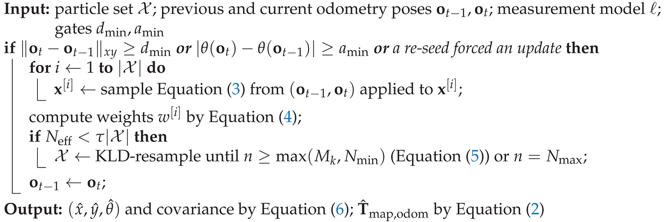
Both pose-tracking backends share one particle filter over the planar pose (Pose2D), with belief . The recursion is the one wired in localization_node.cpp and summarized in Algorithm 1.
Motion Model. OdometryMotionModel implements the sampling form of the odometry model (Thrun et al., 2005). Consecutive odometry poses are decomposed into , with whenever m (pure-rotation guard), and each particle is advanced by the noise-corrupted increment
where draws zero-mean Gaussian noise of variance and are the alpha1–alpha4 parameters.
Weighting. Given a measurement model with log-likelihood (Section 3.3), the correct step of ParticleFilter replaces each weight by
subtracting the per-step maximum for numerical stability. The weights are overwritten rather than multiplied into the previous ones; this coincides with the standard recursion after every resampling step (which leaves uniform weights), and otherwise discards the previous step’s weights, a simplification we note rather than hide.
KLD-Adaptive Resampling. Resampling is triggered only when the effective sample size falls below (resample_threshold). Samples are then drawn with probability proportional to weight and dropped into a histogram with bins of kld_bin_xy in and kld_bin_yaw in . Following Fox (2003), after distinct bins have been occupied the target sample count is
and drawing stops once or , with (kld_err), (kld_z), and (min_particles, max_particles) as parameters. The resampled set receives uniform weights.
Pose Estimate. The reported pose is the weighted mean of with the circular mean of ,
and the covariance carries the weighted planar second moments in and , while z, roll, and pitch are marked unobserved with variance .
| Algorithm 1: One laser2d/ndt3d filter update, as wired in localization_node.cpp |
 |
3.3. Scoring Observations: Likelihood-Field and NDT Measurement Models
A backend differs from the other only through a MeasurementModel, whose single virtual method returns the unnormalized log-likelihood of the current observation given a candidate base pose.
2D Likelihood Field. Laser2DLikelihoodField is the likelihood-field model (Thrun et al., 2005). At construction the occupancy grid (cells with value occupied) is converted into a field holding the Euclidean distance to the nearest occupied cell, computed exactly by the separable squared-distance transform of Felzenszwalb and Huttenlocher (2012) and clamped at likelihood_max_dist. For a scan with ranges at bearings , the model visits every s-th beam, , discards ranges outside , and scores
where is the beam endpoint transformed into the map through composed with the sensor mounting pose.
3D NDT Score. Ndt3DModel scores a 3D point cloud against a Normal Distributions Transform map (Biber and Straßer, 2003; Magnusson et al., 2007). NdtMap voxelizes the prior cloud at resolution ndt_resolution; each voxel v with at least voxel_min_points points stores its mean and the inverse of its covariance after inflating every eigenvalue to at least of the largest. With the 3D lift of the planar particle at the fixed height base_height composed with the sensor pose, the per-particle score over a subsampled cloud (at most max_points points) is
with when falls in an empty voxel and . This is a simplified form of NDT-MCL (Saarinen et al., 2013), which represents both the map and the scan by NDTs; here raw points are scored against the NDT map, a score of the kind that Newton registration optimizes is read out as a particle likelihood, and the 3D backend estimates the same as the 2D one.
3.4. Relocalizing by Branch-and-Bound: Deterministic Kidnapped-Robot Recovery
Recovery from a lost or kidnapped estimate is handled by BranchAndBoundMatcher, a correlative scan matcher (Olson, 2009) bounded by a max-pooled pyramid as in Hess et al. (2016). At construction the likelihood field (clamped at ) is converted into a probability grid and a pyramid of levels (bbs_max_depthD),
where cells outside the grid count as zero; is built by doubling, . A search at center with per-axis half-windows in cells enumerates rotations over ±bbs_angular_window at bbs_angular_step and the symmetric set of integer cell offsets . In the node’s default map-sized mode (bbs_global_window), for a grid is the center of cell and , with the compute cap = bbs_max_linear_window (50 m). Offset then places the robot at the center of cell , so unless the cap binds, the candidate positions are exactly the centers of all grid cells (plus at most one off-grid row or column, which the feasibility rule below removes); when the cap binds, the node logs a warning that relocalization is not global. With bbs_global_window disabled, about the map midpoint for the linear window W = bbs_linear_window. A candidate is feasible when the robot position falls in an on-grid cell with occupancy below 50, i.e. a free or unknown () cell; the feasible set is . (Version 0.1 of the code anchored the roots at without trimming, so it enumerated the asymmetric superset , m to m about the map midpoint for the defaults, and it had no feasibility rule.) For rotation , let be the grid cell of the j-th subsampled endpoint (: every s-th beam with a valid range, as in Equation (7), so can reach ) at the center translation. A node at depth h with anchor covers the offsets and is scored by
where at out-of-grid cells contribute zero, and at a block that lies entirely outside the grid contributes zero while any other anchor is clamped into the grid by . Leaves () carry the exact correlative score , which is the correlative surrogate of Hess et al. (2016); Olson (2009), not the MCL log-likelihood of Equation (7).
The two statements below are not new results. They restate the standard branch-and-bound argument of Hess et al. (2016), who note that the search is exact, returning the same solution as exhaustive search, whenever the score of every inner node upper-bounds the scores of its leaves. We restate it because our search set differs from theirs in three details on which the argument depends: coarse nodes are clamped at the map border, the offset window is trimmed to be symmetric, and infeasible leaves are skipped.
Proposition 1
(Admissible bound; cf. (17)). For every node at depth and every leaf offset , .
Proof.
Fix an endpoint j and let . If the block lies entirely outside the grid, every leaf cell is also outside and contributes zero, so both sides are 0. Otherwise, when is inside the grid is by Equation (9) the maximum of over the block, which contains the leaf cell. When a coordinate of is negative, clamping it to 0 yields a block in that coordinate that contains every in-grid cell of , because ; out-of-grid leaf cells contribute . Hence each endpoint’s term at depth h upper-bounds its term at every leaf of the node, and summing over j gives the claim. (Without the clamp, a coarse node whose corner falls off the map would under-count and could prune the optimum; the implementation comment in bbs.cpp records exactly this case.) □
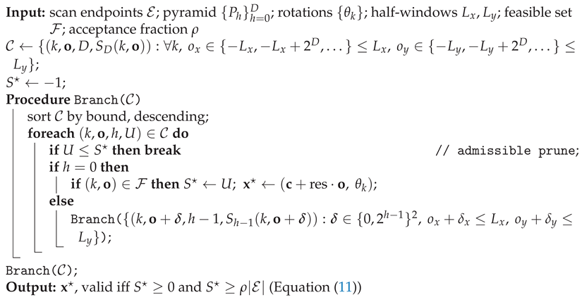
Algorithm 2 tiles with root anchors (and likewise in y), expands nodes depth-first with children visited in decreasing order of their bound, discards any child whose anchor exceeds or , prunes a subtree whenever its bound does not exceed the best feasible leaf score found so far, and skips infeasible leaves.
Corollary 1
(Optimality over the feasible set; cf. Hess et al. 2016). If and , Algorithm 2 returns a candidate with ; ties go to the first maximizer reached.
Proof.
Coverage. Per axis, with : for the root anchor satisfies , so o lies in a root block; every ancestor of the leaf o inside that block has an anchor and is never discarded by the trimming rule. Trimming therefore removes only blocks that contain no offset of , and every candidate of is a leaf of the enumerated tree; conversely every leaf has anchor in each axis and anchor by construction, so the leaves are exactly . Pruning. The incumbent is only ever set from a feasible leaf. A subtree is pruned only when its bound is , and by prop:bbs (which holds for every leaf of a block, feasible or not, inside or not) no leaf below it scores more than . Hence no feasible leaf with a strictly larger score is ever discarded, and the final incumbent attains the maximum over . (With , i.e. no valid range, the code returns an invalid result without searching.) □
The guarantee holds for pyramid values stored in single precision and summed in double: each per-endpoint term at depth h is an exact maximum of leaf values, and the endpoints are summed in the same order at every depth, so monotonicity of rounded addition preserves the inequality. The unit tests check it directly: on randomized small cases the branch-and-bound score equals, bit for bit, that of an exhaustive search over (matchExhaustive), and three negative controls in the suite confirm the test’s power: through a test-only hook (setBoundMutationForTesting) that perturbs the coarse-level bounds, an inflated bound (still admissible) keeps the agreement, whereas a deflated bound () and coarse nodes that use the leaf’s drop rule instead of the clamp, the inadmissible bound of the proof’s remark, are both detected. It is optimality on the rotation–translation lattice only, not over continuous poses, and for the correlative surrogate , not for the pose posterior; it is not optimal localization in any statistical sense. In map-sized mode it is global over the grid’s cell centers whenever the cap does not bind. The match is accepted only when
with = bbs_min_score_fraction and the number of valid endpoints used. The search is deterministic and therefore reproducible in a unit test. On maps with repeated structure a single accepted optimum can be a look-alike place (Section 4), so the node does not commit it directly; it verifies it over several scans (Section 3.5).
| Algorithm 2: Branch-and-bound global relocalization (bbs.cpp) |
 |
3.5. Verifying a Relocalization over Several Scans
RelocalizationVerifier turns the single-scan decision into a multi-hypothesis one, a simple instance of the established practice of tracking several global-localization hypotheses until later observations separate them (García et al., 2023; Gao et al., 2019). Hypotheses. On the first scan the branch-and-bound search keeps up to K = bbs_verify_top_k distinct modes instead of one: two leaves belong to the same mode when they lie within bbs_verify_nms_xy (1 m) and bbs_verify_nms_yaw (0.35 rad) of each other, and only the higher-scoring one is kept (greedy non-maximum suppression). Pruning uses the K-th kept score in place of , so the first mode is still the exact optimum of Corollary 1; the lower modes are the best non-suppressed leaves, without that guarantee, because greedy suppression depends on the visiting order. Every mode that passes Equation (11) becomes a hypothesis i with a uniform prior. Evidence. On each later scan every hypothesis is moved by the odometry increment and re-matched by a small branch-and-bound search (±bbs_verify_track_linear_window = 0.3 m, ±0.1 rad, exact ties resolved toward the prediction). With the per-beam score of that re-match, the log-weights and the normalized evidence score are
with = bbs_verify_evidence_gain; a hypothesis whose re-match window holds no feasible pose dies. Decision. After M = bbs_verify_scans scans (the first included) the best hypothesis is committed only if = bbs_verify_min_posterior and its mean f passes ; if no hypothesis reaches , the node logs the place as ambiguous, does not touch the particle set, and retries from the next scan. is a temperature: Equation (12) treats per-scan scores as independent evidence, which beams are not, so is a normalized heuristic evidence (confidence) score, not a Bayesian posterior and not a calibrated probability; its gain was selected for few false accepts on a separate run (below), not so that matches observed error rates. The code keeps the name posterior for (RelocHypothesis::posterior, bestPosterior(), and the CSV column best_posterior) and for its threshold (min_posterior, ROS parameter bbs_verify_min_posterior); the node’s log messages and PARAMS.md also use the word posterior, and PARAMS.md calls the value a probability. In this paper these identifiers and words all denote the evidence score and its threshold, not a calibrated probability. While verification runs, an existing particle set keeps tracking unchanged; a committed pose re-seeds the filter with a Gaussian of standard deviation . With the rule reduces exactly to the single-scan test (a unit test checks this). The defaults , , , were chosen on a separate parameter-selection run (called calib in the code) whose maps and poses are disjoint from the study of Section 4 (seed 20261105): experiments/select_verify_params.py replays the decision rule over , , , and takes the configuration with the fewest false accepts, then the most correct accepts. On the 200 parameter-selection queries it gives 163 correct accepts and 0 false accepts (9 ambiguous), against 160 and 12 for the single-scan rule.
3.6. Fusing IMU, LiDAR, and GNSS: A 15-State Error-State Kalman Filter
The fusion3d backend runs Eskf, which follows the quaternion error-state formulation of Solà (2017). The nominal state carries position , velocity , orientation , and accelerometer and gyroscope biases ; the error state is with a local angular error .
Prediction. On each IMU sample with period , let , , , and with . The nominal state and error covariance evolve as
where is the exponential, is the identity except for the blocks
and the process noise
is built from sigma_acc, sigma_gyro, sigma_acc_bias, and sigma_gyro_bias; denotes the rotation matrix of a quaternion.
Correction, Injection, Reset. Two updates share the Kalman gain,
updatePose applies a 6-DoF pose from NDT registration with selecting and residual , with (pose_pos_std, pose_rot_std); the node applies it only when PCL’s NDT converged with fitness at most ndt_max_fitness. updatePosition applies a 3-DoF GNSS fix, converted from WGS-84 through ECEF to a local ENU frame about a datum (the first accepted fix unless use_datum fixes one), with selecting and taken from the fix covariance (horizontal variances floored at , vertical at 1). After each update the error is injected, additively for and as for orientation, and the error mean is reset to zero. The implementation uses the simple covariance update of Equation (14). By default it omits the reset Jacobian (it takes ), a common first-order simplification of the full formulation in Solà (2017); the option reset_jacobian applies with after each injection, and Section 4.3 measures its effect on consistency.
3.7. Initializing and Diagnosing: Making Every Precondition Observable
All backends accept a PoseWithCovarianceStamped on /initialpose: the MCL backends spread a Gaussian particle cloud at the supplied mean and covariance, and the fusion backend loads it as its nominal state. Automatically, laser2d runs Algorithm 2 before its first pose when try_global_localization is set, or on demand through the ~/global_localization service (the matcher is constructed lazily at the first call). fusion3d auto-initializes once it holds both an attitude, roll and pitch from the first IMU specific force and heading from initial_yaw,
and a position from the first GNSS fix that passes the gate (gnss_min_status, gnss_max_pos_cov).
Because a localization node that silently does nothing is the dominant first-run frustration, four diagnostic mechanisms accompany the estimators: (i) ndt3d and fusion3d abort construction with an actionable error when map_pcd_path is empty or fails to load; (ii) every callback that cannot yet act emits a rate-limited warning naming the unmet precondition and the remedy; (iii) a 10 s startup watchdog reports each silent mandatory input together with its live publisher count, separating “no publisher” from “publisher present but QoS-incompatible”; and (iv) the GNSS gate and the NDT update log each rejection with the measured value against the violated threshold. Every tunable is a declared ROS 2 parameter documented one-to-one in PARAMS.md (Appendix B). These mechanisms carry no algorithmic weight; they exist so that a misconfiguration is diagnosable from the console log alone, in the spirit of the logging infrastructure Nav2 relied on in its long-duration field experiment (Macenski et al., 2020).
4. Experiments
We validate PRISM-Loc at the level of correctness and closed-loop behavior, not field accuracy. Section 4.1 describes the test suite and the six synthetic closed-loop experiments, Section 4.2 reports their results, and Section 4.3 isolates the contribution of individual mechanisms using the same committed runs. All data in this section are synthetic, and we make no accuracy claim about physical robots.
4.1. Experimental Setup
Correctness Tests. The suite comprises 63 GoogleTest cases across the four packages: 42 in prism_loc_core (both MCL backends and global recovery), 15 in prism_loc_fusion (the ESKF), 4 in the prism_loc adapter layer, and 2 in prism_loc_fusion_ros. The motion model is checked deterministically (zero-command and pure-translation cases) and statistically (the mean of noisy samples approximates the commanded motion); both measurement models are checked for the monotonicity a likelihood must satisfy (the true pose out-scores a displaced one); resampling, the weighted-mean estimate, the grid and NDT-map primitives, and branch-and-bound recovery of a single-scan kidnapped pose (with rejection of an empty scan) are tested directly, the latter also on a 40 m×30 m map with the pose 17 m from the center, together with the symmetric window, the compute cap, the rejection of occupied and off-map candidates, and bit-exact agreement with exhaustive search (Corollary 1) with three negative controls that perturb the bound; the top-K search and the verifier of Section 3.5 are tested on twin rooms that are identical within sensor range: the first mode equals the single-best match, both twins are returned with equal score, a scan that fools the single-scan rule (an unmapped box beside the robot matches a mapped box in the other twin) is resolved once driving brings a distinguishing pillar into range, a place that nothing in range distinguishes is reported ambiguous rather than committed, an unambiguous place is accepted at the true pose, and reproduces the single-scan result; two integration tests close the laser2d and ndt3d loops until convergence to ground truth. The ESKF is pinned for rest under a static IMU, constant-acceleration kinematics, measurement pull-in, and tracking of a moving target from a wrong initial guess; exponential/logarithm round trips, geodetic ENU round trips, and the Equation (2) composition are verified separately, and RNG tests assert that equal seeds reproduce identical sequences; two tests pin the optional ESKF reset Jacobian. Two CI jobs guard the boundary from both sides: a core job builds the two cores with plain CMake and runs ctest with only a compiler and Eigen, and a ROS job runs colcon build and colcon test for all four packages in a ros:humble container.
Synthetic Closed-Loop Protocol. Six drivers under experiments/ compile the actual core sources directly with g++ and Eigen (no ROS, no CMake) and generate their own worlds, scans, and inertial streams, with all randomness derived from fixed compile-time seeds. The sensor-noise models match the filters’ assumptions by construction, so the experiments demonstrate behavior rather than benchmark accuracy.
- MCL tracking. A grid at 0.1 m/cell (room border plus two interior pillars) hosts a robot driven around a closed oval loop with semi-axes 3.6 m and 2.6 m for 65 s at 10 Hz (650 steps). Each step ray-casts a 180-beam scan at the true pose and synthesizes drifting odometry from noise-corrupted increments under the laser2d.yaml model (). The filter, with every parameter from laser2d.yaml, is seeded with a broad Gaussian prior ( m, 0.4 rad) at the true start and updated as in Algorithm 1 with . Seeds: 101, 202, 303.
- BBS relocalization. On an asymmetric room (two interior wall stubs break the four-fold symmetry, the world of the BBS unit test), poses are drawn uniformly over free space with uniform yaw, and one 180-beam scan is ray-cast per pose. To span easy to hard cases, each beam is replaced with a uniform-random spurious range with a per-query probability drawn uniformly in , modeling people, glass, and objects absent from the map. The real matcher runs with the bbs_* defaults ( m, at 0.0175 rad , , bbs_max_beams, which for a 180-beam scan gives stride 1, so all 180 beams are scored), centered on the room, so its window covers the whole map. The committed CSV was produced by the first release of the matcher; re-running the driver against the current matcher (symmetric window, feasibility rule) reproduces every column except wall-clock latency. Seed: 20240607.
- ESKF under aiding dropout. The real Eskf runs over a 60 s 3D trajectory, a horizontal figure-eight , with and a m altitude oscillation. The analytic specific force and angular rate are corrupted with exactly the white-noise densities and constant biases the process model assumes (fusion3d.yaml defaults), plus fixed true biases the filter must estimate from zero. The IMU runs at 200 Hz, a simulated NDT source delivers 6-DoF poses at 10 Hz and a simulated GNSS source positions at 1 Hz, with noise matched to the filter’s ; both aiding streams are withheld for s. Seed: 20240517.
- BBS on large maps. Square warehouse-like grids of side 20, 40, and 80 m at 0.1 m/cell carry border walls, repeated shelf rows (0.5 m deep at a 6 m pitch with 1–2 random gaps each) and random 0.4 m pillars; the repetition deliberately creates look-alike places. Kidnapped poses are drawn uniformly over free space and stratified into 60 inside and 60 outside the set that the first release searched ( m to m about the map center; the 20 m map lies entirely inside it). One 180-beam, 30 m-range scan per pose receives the room study’s clutter model, and the first-release matcher (a verbatim copy, centered on the map midpoint with m) and the current map-sized matcher process the identical scan. Seed: 20260928.
- Multi-scan verification. On the maps, poses, and first scans of the large-map study (same seed and draw order, so the single-scan rows reproduce it exactly), the robot then drives a short random trajectory: 0.3 m forward steps with heading changes, an in-place turn when a step would leave free space, and one scan per step with the query’s clutter fraction. The verifier receives odometry increments corrupted by m per axis and rad. Success is judged against the true pose at the scan where the method commits. Seed: 20260928 (study); 20261105 for the parameter-selection run of Section 3.5.
- ESKF Monte Carlo NEES. runs of the ESKF scenario above in which the initial position, velocity, and attitude errors and the true IMU biases are drawn from the filter’s prior , and the true biases then random-walk with the filter’s bias process noise, so that the prior, the sensor and bias noise, and the aiding noise all match the filter’s model; the one unmodeled effect is that the IMU samples an analytic trajectory, whose integration between samples the zero-order-hold process model does not represent exactly. Every 0.5 s we average the normalized estimation error squared over the runs, for the full 15-D error and for each 3-D block, and compare it with the two-sided 95% interval for n degrees of freedom (Bar-Shalom et al., 2001). The shipped filter and the reset-Jacobian variant process identical data. No parameter was tuned on these runs. Seeds: 20260929 plus the run index, and 20261029 plus the run index for the bias random walk.
Baselines, Metrics, and Hardware. No external baseline is run: neither a tracker such as nav2_amcl, Beluga (Puga et al., 2024), MH-AMCL (García et al., 2023), or hdl_localization (Koide et al., 2019), nor a global localizer such as hdl_global_localization (Koide, 2021) or CBGL (Filotheou, 2024), nor another multi-hypothesis verifier (Gao et al., 2019). The synthetic worlds are designed to exercise PRISM-Loc’s own cores, every comparison below is between configurations of PRISM-Loc itself, and a comparative study on real and public data is left to future work (Section 5). We report position error (Euclidean, m) and absolute yaw error against synthetic ground truth, BBS success rate (position error m and yaw error ), acceptance and false-accept counts at the threshold of Equation (11), windowed RMSE, the envelope, and Monte Carlo NEES for the ESKF, and BBS wall-clock latency. All accuracy numbers are deterministic; latency is machine-dependent and was measured single-threaded on the machine that produced the committed CSV.
4.2. Main Results
MCL Tracking and KLD Adaptation. Figure 2 and Table 3 show that after convergence ( s, across all three seeds) the laser2d filter holds a mean position error of 0.105 m (max 0.29 m) and a mean yaw error of 0.032 rad, i.e. 1.8∘ (max 0.18 rad), with little spread across seeds ( m over per-seed means). The KLD bound (Equation (5)) sizes the set to the posterior: it starts at the 2000-particle ceiling under the broad prior, collapses to the 500-particle floor after the first post-convergence update, and holds there for the rest of the loop, a reduction in per-update likelihood evaluations once the posterior is concentrated.
Global Relocalization. Of the 100 kidnapped-robot queries, 97 succeed (Table 4); over all queries the recovered pose has median position error 0.037 m (95th percentile 0.072 m) and median yaw error 0.48∘ (95th percentile 1.74∘), consistent with the 0.1 m grid and rotation lattice. Figure 3 shows that the score fraction of Equation (11) is an informative confidence signal: the three failures score in – with more than 3 m and roughly – error, all below , so the default threshold yields zero false accepts while accepting 78 matches, all correct, and conservatively rejecting 19 correct fixes. The median score fraction is 0.632 and successes span –, so three low-scoring successes overlap the failure band. Median full-map query latency is 37.65 ms.
ESKF Fusion. With full aiding the windowed position RMSE is 0.016 m (Table 4). During the 10 s blackout the filter dead-reckons on the IMU alone and the RMSE rises to 0.125 m, with a peak error of 0.256 m at s at the end of the blackout; the first aiding cycle brings the error back to 0.015 m by s, and the post-dropout RMSE is 0.009 m (Figure 4). The filter’s own bound inflates from roughly 0.03–0.04 m under full aiding to 0.663 m and stays above the true error at every logged sample, i.e. the reported position covariance is not overconfident on this single seeded run. This is a one-sided envelope check on one run; the NEES study below is the consistency test.
Relocalization on Large Maps. Table 5 moves the kidnapped-robot study to maps larger than the room. For poses outside the set the first release searched, that matcher succeeds on only 2 of 60 queries on the 40 m map and 0 of 60 on the 80 m map, and at it accepts a wrong in-window pose on 39 and 51 of them; the map-sized matcher recovers 50 and 41 of the same 60 poses. Inside that set the two matchers perform alike, as they should. The map-sized window does not, however, make acceptance safe. At the current matcher accepts a wrong pose on 6 of 120 queries on the 40 m map and 15 of 120 on the 80 m map (first release: 43 and 57). Of these 21 false accepts, 13 are flips and none is closer than 4.95 m to the truth; they are look-alike aisles, not near misses. No threshold removes them cheaply: the highest-scoring false match on the two large maps has score fraction 0.71, and only 94 of the 198 successes score above it. The feasibility rule does act: the first release returned a pose inside an obstacle or off the map on 8 of its 300 queries, the current matcher on none. Global coverage also costs time: the median query takes 29 ms on the 20 m map but 1526 ms on the 80 m map, with a 95th percentile of 6374 ms under heavy clutter.
Verification against Aliasing. Table 6 replaces the single-scan acceptance with the verifier of Section 3.5 on the same queries. False accepts fall from 6 of 120 to 0 of 120 on the 40 m map and from 15 to 1 of 120 on the 80 m map; pooled over both maps the false-accept rate falls from 21 of 240 [5.8, 13.0] % to 1 of 240 [0.1, 2.3] % (95% Wilson score intervals, Wilson 1927). Of the 21 single-scan false accepts, 9 become correct fixes, 8 end as ambiguous, and 3 as no candidate; 1 remains a false accept. That residual case is a flip on the 80 m map, 34.7 m from the truth, which held 0.969 of the evidence score after nine scans: verification makes a confident wrong pose rarer, it does not rule it out. The price is small in correct fixes and moderate in time. The verifier commits 242 correct poses against 241 for the single scan over all 300 queries; it loses 8 fixes the single scan had (2 ambiguous, 6 rejected because the mean score fraction over the nine scans falls below , these six all at clutter fractions of at least 0.66) and gains 9. Its median decision takes 1622 ms on the 80 m map against 1247 ms for the single scan in the same run (three concurrent workers, so not comparable with the single-threaded latencies above), dominated by the wider top-8 search, and it needs the robot to move for eight more scans; a stationary robot in a look-alike place stays ambiguous by design.
ESKF Consistency. The NEES test gives a negative verdict (Table 7, Figure 5): the filter is overconfident. Its time-averaged full-state NEES is 18.05 against 15 degrees of freedom, and at single epochs the run average lies inside the 95% interval at only 31 of 120 epochs and above it (overconfident) at the other 89; it is never below it. The blocks locate the problem. Attitude is the worst block (above at 47 epochs, peak 5.91 against an upper limit of 3.50); position (inside at 104 of 120 epochs) and velocity are overconfident mainly during and just after the aiding dropout; both bias blocks are consistent (inside at 116 and 120 of 120 epochs). The published orientation covariance is therefore too small, and the position covariance is too small while aiding is absent. A first version of this study held the true biases constant while the filter injects bias random-walk noise; with that mismatch both bias blocks read as underconfident, and with the bias random walk added to the truth they are consistent.
Table 7.
Monte Carlo NEES of the ESKF ( runs, 120 epochs at 2 Hz after ; initial error and true IMU biases drawn from ). Band: two-sided 95% interval for the run-averaged NEES; a consistent filter keeps about 95% of epochs inside it. In / above / below count epochs for the shipped filter (); the last column is the time-averaged NEES with the reset Jacobian enabled on identical data (data/eskf_nees.csv, experiments/eskf_nees.cpp).
Table 7.
Monte Carlo NEES of the ESKF ( runs, 120 epochs at 2 Hz after ; initial error and true IMU biases drawn from ). Band: two-sided 95% interval for the run-averaged NEES; a consistent filter keeps about 95% of epochs inside it. In / above / below count epochs for the shipped filter (); the last column is the time-averaged NEES with the reset Jacobian enabled on identical data (data/eskf_nees.csv, experiments/eskf_nees.cpp).
| Error block (dof) | 95% band | Mean NEES, | In / above / below | Mean NEES, reset G |
|---|---|---|---|---|
| Full state (15) | [13.95, 16.09] | 18.05 | 31 / 89 / 0 | 18.04 |
| Position (3) | [2.54, 3.50] | 3.10 | 104 / 15 / 1 | 3.10 |
| Velocity (3) | [2.54, 3.50] | 3.15 | 94 / 25 / 1 | 3.15 |
| Attitude (3) | [2.54, 3.50] | 3.48 | 73 / 47 / 0 | 3.48 |
| Accel. bias (3) | [2.54, 3.50] | 3.09 | 116 / 4 / 0 | 3.09 |
| Gyro bias (3) | [2.54, 3.50] | 3.12 | 120 / 0 / 0 | 3.12 |
4.3. Ablation Studies
The committed runs also isolate the effect of four mechanisms. All numbers below are recomputed from the same CSVs; no additional experiment was run for this section.
Acceptance Threshold. Table 8 sweeps over the recorded score fractions. Without the gate () all three failures would re-seed the filter at a wrong pose; any removes every false accept, and the shipped trades 19 rejected correct fixes for a margin of above the highest-scoring failure. Because a rejected match merely waits for the next scan, whereas a false accept silently corrupts the posterior, we keep the conservative default; would have accepted 16 more correct fixes on this data.
Clutter. Table 9 shows how clutter affects the matcher. Below a clutter probability of every query succeeds and is accepted; in the top third the pose is still recovered in 30 of 33 cases with an unchanged median error, but the median score fraction falls to 0.353, so only 11 are accepted. Clutter therefore degrades the matcher’s confidence much faster than its accuracy, and the gate absorbs the difference; all three failures occur in this top third.
KLD Adaptation and Aiding. Replacing KLD adaptation with a fixed set at the 2000-particle ceiling would cost four times the steady-state likelihood evaluations of the 500-particle floor; averaged over each whole run, including the initial transient, the adaptive set holds 526.9 particles, 3.8× fewer than the ceiling, with the accuracy of Table 3. The dropout window acts as an ablation of both aiding streams: removing NDT and GNSS updates raises position RMSE from 0.016 m to 0.125 m over 10 s, and restoring them recovers 0.009 m, so the growth is the bounded drift of IMU-only integration from which the filter recovers within one aiding cycle.
Reset Jacobian. Enabling reset_jacobian on identical data changes the run-averaged NEES of Table 7 by at most 0.026 at any epoch and in any block, and leaves every in/above/below count unchanged, so the omitted reset Jacobian is not the source of the inconsistency; with 10 Hz pose updates the injected attitude corrections are small, which is consistent with . We have not isolated the cause; candidates are the zero-order-hold discretization of the synthetic IMU, which the process model does not account for, and the first-order treatment of the attitude–bias coupling.
5. Discussion and Limitations
What the Factoring Buys. Because the MCL core is written against one MeasurementModel interface, the 2D and 3D backends share the motion model, weighting, KLD resampling, estimate, and every test of those components; adding a backend means adding one likelihood function. This is the same benefit that Beluga’s shared core provides (Puga et al., 2024), and we report it as a property of the artifact rather than as a contribution. Because the cores are middleware-free, every equation of Section 3 is exercised by deterministic tests and by the closed-loop drivers of Section 4 without a ROS installation, which is also what makes the evaluation reproducible bit for bit from the repository.
Cost Analysis. The per-update cost of the MCL backends is linear in the particle count and in the number of scored beams or points (Equations (7) and (8)); KLD adaptation keeps the former at the 500-particle floor once the posterior is concentrated (Figure 2). The branch-and-bound matcher’s cost is data-dependent through pruning: on the synthetic room a full-map query took a median of 37.65 ms (min 8.77 ms, 95th percentile 106.07 ms) on the machine that produced the committed data, and it runs only when relocalization is requested, not every scan. Because the map-sized window grows with map area, so does the cost: on the 80 m map of Table 5 the median query takes 1526 ms, which is acceptable for an on-demand recovery but not for per-scan use; bbs_max_linear_window bounds it at the price of global coverage. Keeping the top eight modes weakens the pruning, and the local re-matches of the later scans are cheap, so in Table 6 a verified decision costs roughly 1.3 times the single-scan query on the 80 m map, plus the time to drive eight more scans. The ESKF step is a fixed covariance propagation per IMU sample.
Limitations. PRISM-Loc is a systems paper that integrates established components, and its scope is deliberately bounded. (i) Planar state in the MCL backends. Both particle-filter backends estimate ; ndt3d evaluates a full 3D Gaussian-voxel map from that planar pose at a fixed base height, which suits wheeled robots on locally flat floors but does not track roll, pitch, or vertical motion. Full state exists only in fusion3d; existing particle-filter packages already estimate a full 3D pose against NDT or point-cloud maps (Puga et al., 2024; Ekumen, Inc., 2022; Watanabe, 2016). (ii) 2D-only relocalization with a heuristic verification. Algorithm 2 operates on a 2D occupancy pyramid; ndt3d and fusion3d rely on an operator-supplied or GNSS-derived initial pose and local tracking. The search window is sized from the map and restricted to non-occupied cells. On maps with repeated structure the score fraction of Equation (11) alone does not separate look-alike places: a single scan accepted a wrong pose on 6 of 120 (40 m) and 15 of 120 (80 m) synthetic queries, and no single threshold removes these on the two maps together without rejecting more than half of the correct fixes. Multi-scan verification (Section 3.5) reduces them to 0 and 1, but it is a heuristic: its evidence score (named a posterior in the code) treats correlated scans as independent evidence behind a tuned temperature and is not a calibrated probability, its parameters were tuned on one synthetic generator (on disjoint seeds), the one residual false accept held 0.969 of the evidence score, it can only choose among the K modes of the first scan, it needs the robot to move, and the top-8 search is slower than the single-best one. It was evaluated only on synthetic worlds with simulated odometry. Relocalization runs only at startup or on a service call; unlike reliability-aware MCL (Akai, 2023), no loss detector triggers it. Beyond the compute cap (100 m per axis by default) the search is no longer global, which the node reports at startup. (iii) No time-offset or extrinsic estimation. The ESKF treats the LiDAR/GNSS-to-IMU time offset and the LiDAR–IMU extrinsic as known inputs. (iv) Loosely-coupled LiDAR update and an inconsistent covariance. In fusion3d, PCL NDT produces a 6-DoF pose measurement that the ESKF fuses as a loosely-coupled update, which keeps the filter core independent of the registration engine but forgoes the accuracy of tightly-coupled formulations such as FAST-LIO (Xu and Zhang, 2021). The filter is also not NEES-consistent on our synthetic scenario (Table 7): it is overconfident, most of all in attitude and, while aiding is absent, in position and velocity, whereas its bias blocks are consistent; the optional reset Jacobian of Solà (2017) does not change this. We therefore regard fusion3d as experimental: consumers should treat the published orientation covariance, and the position covariance during aiding outages, with caution until the cause is found. (v) Single static map. All backends assume one prior map of a static world, loaded once, with no online map update or change detection. (vi) No external baseline and no real data. The evaluation of Section 4 is deterministic unit and integration testing plus a seeded synthetic study whose worlds and sensor-noise models match the filters’ assumptions by construction. Every comparison in it is internal, between configurations of PRISM-Loc: we have not compared the trackers with nav2_amcl, Beluga (Puga et al., 2024), or MH-AMCL (García et al., 2023), the relocalizer with hdl_global_localization (Koide, 2021), the recovery tooling of lidar_localization_ros2 (Sasaki, 2026), CBGL (Filotheou, 2024), or the method of Zhang et al. (2026), or the verifier with the multiple-hypothesis tracker of Gao et al. (2019). The study therefore establishes that each core behaves as specified in closed loop; it does not establish accuracy on a physical robot, competitiveness with these systems, or that the false-accept reduction transfers to real maps and real odometry. We have not measured trajectory error on physical or public datasets. The planned evaluation runs the three backends and at least nav2_amcl and one external global-localization method on public LiDAR sequences, including one with repeated structure, and reports absolute and relative trajectory error (ATE/RPE) following the TUM RGB-D conventions (Sturm et al., 2012) on the per-backend map→odom estimates, together with relocalization success and false-accept rates. Until then we make no accuracy claim.
Future Work. Extending the MCL core to a 6-DoF particle state or coupling it to an external attitude source, re-admitting new candidates during verification and a principled (correlation-aware) evidence model for the 2D relocalizer, a loss detector that triggers it, a 3D branch-and-bound front end such as 3D-BBS (Aoki et al., 2024) or a place-recognition front end for the 3D backends, a diagnosis of the ESKF’s attitude overconfidence, joint time-offset and extrinsic estimation in the ESKF, and the external-baseline evaluation above are the next steps on the roadmap.
6. Conclusions
We presented PRISM-Loc, a LiDAR localization stack whose contribution is a specific integration of established components rather than a new algorithm: three known estimator families, likelihood-field MCL, NDT-MCL (Saarinen et al., 2013), and an error-state Kalman filter fusing LiDAR, IMU, and RTK-GNSS, sit behind a single ROS 2 topic and TF contract, so that a 2D LiDAR, a 3D LiDAR, or a sensor-fused configuration is a deployment choice rather than a switch to a stack with a different interface. Each estimator is a pure C++ core with no dependence on the middleware runtime, the two MCL backends share one predict–weight–resample core that differs only in its measurement model, as in existing MCL libraries (Puga et al., 2024), and laser2d relocalizes deterministically by branch-and-bound (Hess et al., 2016) over a map-sized window of non-occupied cells and verifies the top candidates over several scans before committing, a simple instance of established multi-hypothesis verification that can report a place as ambiguous. Seeded synthetic experiments show that the assembled pipelines behave as intended in closed loop, and they also expose two open problems that we report rather than hide: on large maps with repeated structure a single scan admits wrong poses, which multi-scan verification makes rare (1 of 240 synthetic queries) but does not rule out, and the ESKF covariance is overconfident, mainly in attitude. An evaluation on real and public data against external baselines remains future work. PRISM-Loc is released under the Apache-2.0 license at https://github.com/kjungmo/prism_loc.
Appendix A. Reproduction
Every number and figure of Section 4 regenerates from the repository alone. The drivers and the core test suites need only a C++17 compiler and the Eigen 3 headers (Debian/Ubuntu packages g++, libeigen3-dev); the unit tests additionally use GoogleTest (libgtest-dev). ROS 2 Humble is required only for the two node packages, which continuous integration builds in a ros:humble container (.github/workflows/ci.yml). From the repository root:
CORE="-I prism_loc_core/include -I prism_loc_core/test -I /usr/include/eigen3"
g++ -O2 -std=c++17 $CORE prism_loc_core/src/*.cpp \
experiments/mcl_tracking.cpp -o /tmp/exp_mcl && /tmp/exp_mcl
g++ -O2 -std=c++17 $CORE prism_loc_core/src/*.cpp \
experiments/bbs_relocalization.cpp -o /tmp/exp_bbs && /tmp/exp_bbs
g++ -O2 -std=c++17 -I prism_loc_fusion/include -I /usr/include/eigen3 \
prism_loc_fusion/src/*.cpp experiments/eskf_fusion.cpp -o /tmp/exp_eskf
/tmp/exp_eskf > docs/paper/data/eskf_track.csv
g++ -O2 -std=c++17 $CORE -I experiments prism_loc_core/src/*.cpp \
experiments/legacy/bbs_v01.cpp experiments/bbs_largemap.cpp \
-o /tmp/exp_bbs_large && /tmp/exp_bbs_large # about 7 min
g++ -O2 -std=c++17 -I prism_loc_fusion/include -I /usr/include/eigen3 \
prism_loc_fusion/src/*.cpp experiments/eskf_nees.cpp -o /tmp/exp_nees
/tmp/exp_nees
g++ -O2 -std=c++17 $CORE prism_loc_core/src/*.cpp \
experiments/bbs_verify.cpp -pthread -o /tmp/exp_bbs_verify
/tmp/exp_bbs_verify calib 10 # parameter-selection log
python3 experiments/select_verify_params.py --check
/tmp/exp_bbs_verify study 3 # verification study
python3 docs/paper/make_study_tables.py # generated study tables
python3 docs/paper/check_numbers.py # recompute every quoted statistic
All randomness derives from fixed compile-time seeds (Table A1), so every CSV column is bit-for-bit reproducible except the wall-clock time_ms latency columns of the two BBS experiments. We re-ran all three drivers from the sources of this commit while preparing this version: mcl_tracking.csv, mcl_particles.csv, and eskf_track.csv were byte-identical to the committed files, and bbs_relocalization.csv matched in every column except time_ms. On that re-run machine (AMD Ryzen 5 5500GT, single thread) the median BBS query latency was 10.26 ms against the 37.65 ms of the committed CSV, which illustrates why latency is reported as machine-dependent; the re-run CSV is committed under docs/paper/data/rerun_2026-09-28/. After the matcher gained its symmetric window and feasibility rule we re-ran the room study once more against the current code (bbs_relocalization_fixbbs.csv in the same directory): again every column except time_ms is identical to the committed CSV, with a median latency of 9.90 ms on the same re-run machine. The guard script docs/paper/check_numbers.py recomputes each headline statistic from the committed CSVs and fails if a number quoted in the LATEX sources, including this package, no longer matches.
Table A1.
Experiment drivers, fixed seeds, and committed artifacts. Drivers live under experiments/; CSVs under docs/paper/data/ (copied to data/ in this package).
Table A1.
Experiment drivers, fixed seeds, and committed artifacts. Drivers live under experiments/; CSVs under docs/paper/data/ (copied to data/ in this package).
| Driver | Seed(s) | Figures / tables | CSV(s) |
|---|---|---|---|
| mcl_tracking.cpp | 101, 202, 303 | Figure 2, Table 3 | mcl_tracking.csv, mcl_particles.csv |
| bbs_relocalization.cpp | 20240607 | Figure 3, Table 4,Table 8,Table 9 | bbs_relocalization.csv |
| eskf_fusion.cpp | 20240517 | Figure 4, Table 4 | eskf_track.csv |
| bbs_largemap.cpp | 20260928 | Table 5 | bbs_largemap.csv |
| bbs_verify.cpp | 20260928 | Table 6 | bbs_verify.csv |
| parameter selection | 20261105 | Section 3.5 | bbs_verify_calib.csv, .._selection.csv |
| eskf_nees.cpp | 20260929 | Table 7, Figure 5 | eskf_nees.csv |
Appendix B. Parameters
Table A2 lists the defaults used throughout the paper; each is a declared ROS 2 parameter documented one-to-one in PARAMS.md, with deployed overrides in prism_loc/params/laser2d.yaml, prism_loc/params/ndt3d.yaml, and prism_loc_fusion_ros/params/fusion3d.yaml.
Table A2.
Default parameters (from the shipped YAML files; symbols as in Section 3).
Table A2.
Default parameters (from the shipped YAML files; symbols as in Section 3).
| Parameter | Symbol | Default | Used in |
|---|---|---|---|
| min_particles / max_particles | / | 500 / 2000 | Equation (5) |
| resample_threshold | 0.5 | trigger | |
| kld_err / kld_z | / | 0.05 / 2.33 | Equation (5) |
| kld_bin_xy / kld_bin_yaw | – | 0.5 m / 0.17 rad | Equation (5) |
| update_min_d / update_min_a | / | 0.2 m / 0.2 rad | Algorithm 1 |
| alpha1–alpha4 | 0.2 | Equation (3) | |
| max_beams | – | 60 | Equation (7) |
| z_hit / z_rand / sigma_hit | / / | 0.5 / 0.5 / 0.2 m | Equations (7) and (9) |
| likelihood_max_dist | – | 2.0 m | Equation (7) |
| ndt_resolution / voxel_min_points | – | 1.0 m / 5 | Equation (8) |
| max_points / base_height | – | 500 / 0.0 m | Equation (8) |
| bbs_global_window | – | true | Section 3.4 |
| bbs_max_linear_window | 50.0 m | Section 3.4 | |
| bbs_linear_window (if not global) | W | 10.0 m | Section 3.4 |
| bbs_angular_window / bbs_angular_step | – | / 0.0175 rad | Algorithm 2 |
| bbs_max_depth / bbs_max_beams | D / – | 6 / 120 | Equations (9) and (10) |
| bbs_min_score_fraction | 0.4 | Equation (11) | |
| bbs_verify_top_k | K | 8 | Section 3.5 |
| bbs_verify_scans | M | 9 | Section 3.5 |
| bbs_verify_evidence_gain | 40 | Equation (12) | |
| bbs_verify_min_posterior | 0.9 | Equation (12) | |
| bbs_verify_nms_xy / _yaw | – | 1.0 m / 0.35 rad | Section 3.5 |
| bbs_verify_track_*_window | – | 0.3 m / 0.1 rad | Section 3.5 |
| sigma_acc / sigma_gyro | / | 0.01 / 0.001 | Equation (13) |
| sigma_acc_bias / sigma_gyro_bias | / | / | Equation (13) |
| reset_jacobian | false () | Section 3.6 | |
| pose_pos_std / pose_rot_std | / | 0.1 m / 0.05 rad | Equation (14) |
| ndt_max_fitness | – | 2.0 | NDT gate |
| gnss_min_status / gnss_max_pos_cov | / | 0 / 25.0 m2 | GNSS gate |
| transform_tolerance / seed | – | 0.1 s / 42 | Equation (2) / RNG |
Appendix C. Code Map
Table A3 maps each equation and algorithm to the source file that implements it, and Table A4 collects the notation.
Table A3.
Where each equation lives. Paths are relative to the repository root; core/ abbreviates prism_loc_core/src/, fusion/ abbreviates prism_loc_fusion/src/, and node/ and fnode/ abbreviate prism_loc/src/localization_node.cpp and prism_loc_fusion_ros/src/fusion_localization_node.cpp.
Table A3.
Where each equation lives. Paths are relative to the repository root; core/ abbreviates prism_loc_core/src/, fusion/ abbreviates prism_loc_fusion/src/, and node/ and fnode/ abbreviate prism_loc/src/localization_node.cpp and prism_loc_fusion_ros/src/fusion_localization_node.cpp.
| Equation / algorithm | Source |
|---|---|
| Equation (2) (map→odom) | node/, fnode/; tests prism_loc/test/test_tf_math.cpp, prism_loc_fusion_ros/test/test_tf_compose.cpp |
| Equation (3) (motion model) | core/motion_model.cpp |
| Equations (4)–(6) (filter) | core/particle_filter.cpp |
| Algorithm 1 (update order, gates) | node/ (runUpdate, onScan) |
| Equation (7) (likelihood field) | core/measurement_model.cpp, core/occupancy_grid.cpp |
| Equation (8) (NDT score) | core/measurement_model.cpp, core/ndt_map.cpp |
| Equations (9)–(11), Algorithm 2 | core/bbs.cpp; re-seeding in node/ (runRelocalization) |
| Equations (13) and (14) (ESKF) | fusion/eskf.cpp, fusion/so3.cpp, fusion/geodetic.cpp |
| Equation (15), GNSS and NDT gates | fnode/ (attitudeFromAccel, onGnss, onPoints) |
| Corollary 1 check (exhaustive search) | core/bbs.cpp (matchExhaustive); test prism_loc_core/test/test_bbs.cpp |
| Equation (12), Section 3.5 | core/relocalization.cpp (RelocalizationVerifier), core/bbs.cpp (matchGlobalTopK, matchLocal); node runRelocalization; test test_relocalization.cpp |
| Synthetic drivers | experiments/mcl_tracking.cpp, bbs_relocalization.cpp, eskf_fusion.cpp, bbs_largemap.cpp (with legacy/bbs_v01.cpp), eskf_nees.cpp, bbs_verify.cpp (with select_verify_params.py) |
Table A4.
Notation.
| Symbol | Meaning | Symbol | Meaning |
|---|---|---|---|
| set of backends | pose of frame b in frame a | ||
| planar particle pose | particle weight | ||
| measurement log-likelihood | effective sample size | ||
| KLD sample bound, k bins | distance to nearest obstacle | ||
| NDT voxel mean, covariance | BBS pyramid level h | ||
| BBS node score | subsampled scan endpoints | ||
| BBS acceptance fraction | D | BBS pyramid depth | |
| , | BBS offset set, half-windows | feasible BBS candidates | |
| BBS half-window cap | NEES | ||
| ESKF position, velocity, attitude | IMU biases | ||
| ESKF error state | error covariance | ||
| transition, process noise | update Jacobian, noise, gain | ||
| ESKF reset Jacobian |
References
- Saarinen, J.; Andreasson, H.; Stoyanov, T.; Lilienthal, A.J. Normal Distributions Transform Monte-Carlo Localization (NDT-MCL). In Proceedings of the 2013 IEEE/RSJ International Conference on Intelligent Robots and Systems (IROS), Tokyo, Japan, 2013; pp. 382–389. [CrossRef]
- Koide, K.; Miura, J.; Menegatti, E. A Portable Three-Dimensional LiDAR-Based System for Long-Term and Wide-Area People Behavior Measurement. International Journal of Advanced Robotic Systems 2019 , 16. [CrossRef]
- Moore, T.; Stouch, D. A Generalized Extended Kalman Filter Implementation for the Robot Operating System. In Proceedings of the Intelligent Autonomous Systems 13: Proceedings of the 13th International Conference (IAS-13), Cham, 2016; Vol. 302, Advances in Intelligent Systems and Computing, pp. 335–348. [CrossRef]
- Macenski, S.; Moore, T.; Lu, D.V.; Merzlyakov, A.; Ferguson, M. From the Desks of ROS Maintainers: A Survey of Modern & Capable Mobile Robotics Algorithms in the Robot Operating System 2. Robotics and Autonomous Systems 2023 , 168, 104493, [arXiv:cs.RO/2307.15236]. [CrossRef]
- Puga, G.; Espinosa, N.; Hidalgo, M.; García, O.; Paunovic, I. Beluga: A Modern Monte Carlo Localization Package for ROS and ROS 2. In Proceedings of the European Robotics Forum 2024, Cham, 2024; Springer Proceedings in Advanced Robotics, pp. 126–130. [CrossRef]
- ekumen2022belugarepo Ekumen, Inc.. Beluga. GitHub repository Ekumen-OS/beluga, https://github.com/Ekumen-OS/beluga, 2022. Generic C++17 MCL library with ROS AMCL nodes that provide interface parity with nav2_amcl (and amcl); includes likelihood-field, beam, and NDT sensor models and 2D and 3D NDT AMCL nodes for ROS 2; accessed 2026-09-30.
- Autoware Foundation. autoware_pose_estimator_arbiter. Autoware Universe documentation, https://autowarefoundation.github.io/autoware_universe/main/localization/autoware_pose_estimator_arbiter/, 2024. Accessed 2026-09-30.
- Locus Robotics. fuse. GitHub repository, https://github.com/locusrobotics/fuse, 2018. A ROS framework for sensor fusion using nonlinear least squares optimization; accessed 2026-09-30.
- Blanco-Claraco, J.L. A Flexible Framework for Accurate LiDAR Odometry, Map Manipulation, and Localization. The International Journal of Robotics Research 2025 , 44, 1553–1599, [arXiv:cs.RO/2407.20465]. [CrossRef]
- Macenski, S.; Martín, F.; White, R.; Clavero, J.G. The Marathon 2: A Navigation System. In Proceedings of the 2020 IEEE/RSJ International Conference on Intelligent Robots and Systems (IROS). IEEE, 2020, pp. 2718–2725, [arXiv:cs.RO/2003.00368]. [CrossRef]
- Fox, D.; Burgard, W.; Dellaert, F.; Thrun, S. Monte Carlo Localization: Efficient Position Estimation for Mobile Robots. In Proceedings of the Proceedings of the Sixteenth National Conference on Artificial Intelligence (AAAI/IAAI), Orlando, FL, USA, 1999; pp. 343–349.
- Thrun, S.; Fox, D.; Burgard, W.; Dellaert, F. Robust Monte Carlo Localization for Mobile Robots. Artificial Intelligence 2001 , 128, 99–141. [CrossRef]
- Akai, N. Reliable Monte Carlo Localization for Mobile Robots. Journal of Field Robotics 2023 , 40, 595–613, [arXiv:cs.RO/2205.04769]. [CrossRef]
- García, A.; Martín, F.; Guerrero, J.M.; Rodríguez, F.J.; Matellán, V. Portable Multi-Hypothesis Monte Carlo Localization for Mobile Robots. In Proceedings of the 2023 IEEE International Conference on Robotics and Automation (ICRA). IEEE, 2023, pp. 1933–1939, [arXiv:cs.RO/2209.07586]. [CrossRef]
- Koide, K. hdl_global_localization. ROS package, GitHub repository, https://github.com/koide3/hdl_global_localization, 2021. Global localization service with 2D grid-map branch-and-bound, FPFH+RANSAC, and FPFH+TEASER++ engines; accessed 2026-09-30.
- Sasaki, R. lidar_localization_ros2: Global Localization. Documentation in the lidar_localization_ros2 GitHub repository, https://github.com/rsasaki0109/lidar_localization_ros2/blob/main/docs/global_localization.md, 2026. The repository dates from 2020; this document was added in 2026. Accessed 2026-09-30.
- Hess, W.; Kohler, D.; Rapp, H.; Andor, D. Real-Time Loop Closure in 2D LIDAR SLAM. In Proceedings of the 2016 IEEE International Conference on Robotics and Automation (ICRA), Stockholm, Sweden, 2016; pp. 1271–1278. [CrossRef]
- Gao, H.; Zhang, X.; Yuan, J.; Song, J.; Fang, Y. A Novel Global Localization Approach Based on Structural Unit Encoding and Multiple Hypothesis Tracking. IEEE Transactions on Instrumentation and Measurement 2019 , 68, 4427–4442. [CrossRef]
- Pedrosa, E. iris_lama. GitHub repository, https://github.com/iris-ua/iris_lama, 2019. C++ localization and mapping library whose only dependency is Eigen; accessed 2026-09-30.
- Adurthi, N. Scan Matching-Based Particle Filter for LIDAR-Only Localization. Sensors 2023 , 23, 4010. [CrossRef]
- Zhang, Y.; Guo, Y.; Zheng, J.; Fan, Z.; Jia, X.; Liu, J. Move First, Commit Later: Selective LiDAR-to-BIM Global Initialization via Sequential Consensus with Symmetry-Aware Abstention. arXiv preprint arXiv:2607.17103, 2026, [arXiv:cs.RO/2607.17103]. Concurrent work.
- Dellaert, F.; Fox, D.; Burgard, W.; Thrun, S. Monte Carlo Localization for Mobile Robots. In Proceedings of the Proceedings of the 1999 IEEE International Conference on Robotics and Automation (ICRA), Detroit, MI, USA, 1999; Vol. 2, pp. 1322–1328. [CrossRef]
- Fox, D. Adapting the Sample Size in Particle Filters Through KLD-Sampling. The International Journal of Robotics Research 2003 , 22, 985–1003. [CrossRef]
- Thrun, S.; Burgard, W.; Fox, D. Probabilistic Robotics; MIT Press: Cambridge, MA, USA, 2005.
- Watanabe, A. mcl_3dl. ROS package, GitHub repository, https://github.com/at-wat/mcl_3dl, 2016. 3-D/6-DOF point-cloud Monte Carlo localization; accessed 2026-09-30.
- Martín Rico, F.; Guerrero Hernández, J.M.; Pérez Rodríguez, R.; Peña Narváez, J.D.; García Gómez-Jacinto, A. Open Source Robot Localization for Non-Planar Environments. arXiv preprint arXiv:2309.12744, 2023, [arXiv:cs.RO/2309.12744].
- Biber, P.; Straßer, W. The Normal Distributions Transform: A New Approach to Laser Scan Matching. In Proceedings of the Proceedings of the 2003 IEEE/RSJ International Conference on Intelligent Robots and Systems (IROS), Las Vegas, NV, USA, 2003; Vol. 3, pp. 2743–2748. [CrossRef]
- Magnusson, M.; Lilienthal, A.; Duckett, T. Scan Registration for Autonomous Mining Vehicles Using 3D-NDT. Journal of Field Robotics 2007 , 24, 803–827. [CrossRef]
- Solà, J. Quaternion Kinematics for the Error-State Kalman Filter, 2017, [arXiv:cs.RO/1711.02508]. arXiv:1711.02508 [cs.RO], tutorial/technical report.
- Wan, G.; Yang, X.; Cai, R.; Li, H.; Zhou, Y.; Wang, H.; Song, S. Robust and Precise Vehicle Localization Based on Multi-Sensor Fusion in Diverse City Scenes. In Proceedings of the 2018 IEEE International Conference on Robotics and Automation (ICRA), Brisbane, QLD, Australia, 2018; pp. 4670–4677, [arXiv:cs.CV/1711.05805]. [CrossRef]
- Xu, W.; Zhang, F. FAST-LIO: A Fast, Robust LiDAR-Inertial Odometry Package by Tightly-Coupled Iterated Kalman Filter. IEEE Robotics and Automation Letters 2021 , 6, 3317–3324, [arXiv:cs.RO/2010.08196]. [CrossRef]
- Olson, E.B. Real-Time Correlative Scan Matching. In Proceedings of the 2009 IEEE International Conference on Robotics and Automation (ICRA), Kobe, Japan, 2009; pp. 4387–4393. [CrossRef]
- Aoki, K.; Koide, K.; Oishi, S.; Yokozuka, M.; Banno, A.; Meguro, J. 3D-BBS: Global Localization for 3D Point Cloud Scan Matching Using Branch-and-Bound Algorithm. In Proceedings of the 2024 IEEE International Conference on Robotics and Automation (ICRA). IEEE, 2024, pp. 1796–1802, [arXiv:cs.RO/2310.10023]. [CrossRef]
- Filotheou, A. CBGL: Fast Monte Carlo Passive Global Localisation of 2D LIDAR Sensor. In Proceedings of the 2024 IEEE/RSJ International Conference on Intelligent Robots and Systems (IROS). IEEE, 2024, pp. 3268–3275, [arXiv:cs.RO/2307.14247]. [CrossRef]
- Zhang, M.; Ma, L.; Wu, Y.; Shen, K.; Huang, D.; Leung, H. Tackling the Kidnapped Robot Problem via Sparse Feasible Hypothesis Sampling and Reliable Batched Multistage Inference. IEEE Transactions on Instrumentation and Measurement 2026 , 75, 7504614, [arXiv:cs.RO/2511.01219]. [CrossRef]
- Zou, X.; Li, J.; Wu, W.; Liang, F.; Yang, B.; Dong, Z. Reliable-loc: Robust Sequential LiDAR Global Localization in Large-Scale Street Scenes Based on Verifiable Cues. arXiv preprint arXiv:2411.07815, 2024, [arXiv:cs.RO/2411.07815].
- Felzenszwalb, P.F.; Huttenlocher, D.P. Distance Transforms of Sampled Functions. Theory of Computing 2012 , 8, 415–428. [CrossRef]
- Bar-Shalom, Y.; Li, X.R.; Kirubarajan, T. Estimation with Applications to Tracking and Navigation: Theory, Algorithms and Software; John Wiley & Sons: New York, 2001. [CrossRef]
- Wilson, E.B. Probable Inference, the Law of Succession, and Statistical Inference. Journal of the American Statistical Association 1927 , 22, 209–212. [CrossRef]
- Sturm, J.; Engelhard, N.; Endres, F.; Burgard, W.; Cremers, D. A Benchmark for the Evaluation of RGB-D SLAM Systems. In Proceedings of the 2012 IEEE/RSJ International Conference on Intelligent Robots and Systems (IROS), Vilamoura, Portugal, 2012; pp. 573–580. [CrossRef]
Figure 1.
PRISM-Loc overview. Two middleware-free estimator cores (bottom, C++17 + Eigen only): prism_loc_core runs the MCL loop (OdometryMotionModel → ParticleFilter, corrected by either the Laser2DLikelihoodField or the Ndt3DModel measurement model, plus a branch-and-bound relocalizer), and prism_loc_fusion runs a 15-state ESKF (IMU prediction, corrected by NDT 6-DoF pose and GNSS position updates). The ROS 2 node packages (top) consume the cores upward through ament, select a backend at launch, bridge messages through adapters, and expose one shared contract: a map→odom TF, a pose-with-covariance output, and an /initialpose seed input.
Figure 1.
PRISM-Loc overview. Two middleware-free estimator cores (bottom, C++17 + Eigen only): prism_loc_core runs the MCL loop (OdometryMotionModel → ParticleFilter, corrected by either the Laser2DLikelihoodField or the Ndt3DModel measurement model, plus a branch-and-bound relocalizer), and prism_loc_fusion runs a 15-state ESKF (IMU prediction, corrected by NDT 6-DoF pose and GNSS position updates). The ROS 2 node packages (top) consume the cores upward through ament, select a backend at launch, bridge messages through adapters, and expose one shared contract: a map→odom TF, a pose-with-covariance output, and an /initialpose seed input.
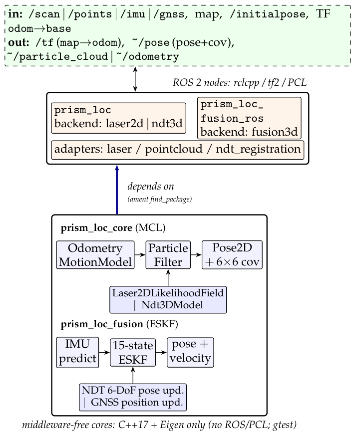
Figure 2.
laser2d closed-loop tracking on synthetic data. A simulated robot drives a closed oval loop (semi-axes 3.6 m and 2.6 m) for 65 s at 10 Hz in a 12 m×10 m grid with two symmetry-breaking pillars; the real ParticleFilter with Laser2DLikelihoodField and KLD resampling is updated exactly as in Algorithm 1. (a) Starting from a broad prior, the filter converges within a few updates; across the three seeds the steady-state ( s) mean position error is 0.105 m (max 0.29 m) and the mean yaw error 0.032 rad (max 0.18 rad). (b) The particle set starts at the 2000-particle ceiling and collapses to the 500-particle floor after the first post-convergence update, where it stays.
Figure 2.
laser2d closed-loop tracking on synthetic data. A simulated robot drives a closed oval loop (semi-axes 3.6 m and 2.6 m) for 65 s at 10 Hz in a 12 m×10 m grid with two symmetry-breaking pillars; the real ParticleFilter with Laser2DLikelihoodField and KLD resampling is updated exactly as in Algorithm 1. (a) Starting from a broad prior, the filter converges within a few updates; across the three seeds the steady-state ( s) mean position error is 0.105 m (max 0.29 m) and the mean yaw error 0.032 rad (max 0.18 rad). (b) The particle set starts at the 2000-particle ceiling and collapses to the 500-particle floor after the first post-convergence update, where it stays.
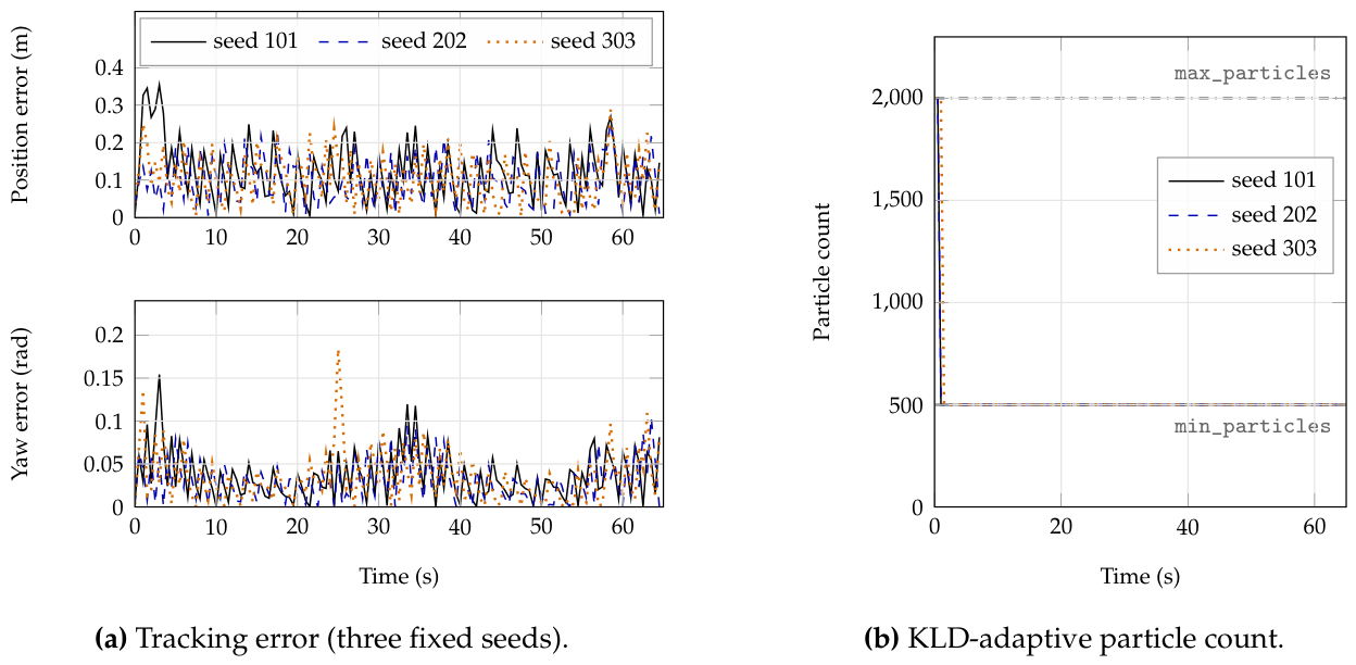
Figure 3.
Branch-and-bound relocalization of a kidnapped robot on synthetic data. Each marker is one of queries in an asymmetric 6 m×6 m room: position error versus the score fraction of Equation (11). Each 180-beam scan is corrupted with a per-query clutter probability drawn uniformly in . Success means position error m (dotted) and yaw error . All three failures score below the default threshold (dashed), so every accepted match is correct (zero false accepts); 19 correct fixes are conservatively rejected.
Figure 3.
Branch-and-bound relocalization of a kidnapped robot on synthetic data. Each marker is one of queries in an asymmetric 6 m×6 m room: position error versus the score fraction of Equation (11). Each 180-beam scan is corrupted with a per-query clutter probability drawn uniformly in . Success means position error m (dotted) and yaw error . All three failures score below the default threshold (dashed), so every accepted match is correct (zero false accepts); 19 correct fixes are conservatively rejected.
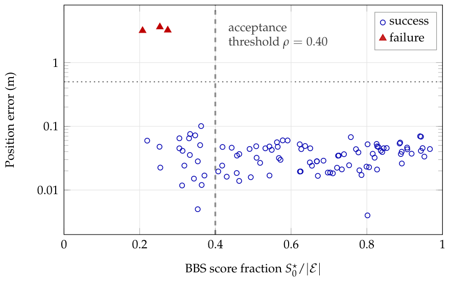
Figure 4.
ESKF fusion under a 10 s aiding dropout on synthetic data. A 200 Hz IMU is fused with 10 Hz NDT-like 6-DoF pose and 1 Hz GNSS-like position updates over a 60 s 3D figure-eight; both aiding streams are withheld for s (shaded). The position error grows to its peak of 0.256 m on dead reckoning alone while the filter’s own bound inflates to 0.663 m, and both collapse within one aiding cycle once updates resume. The bound stays above the true error at every logged sample.
Figure 4.
ESKF fusion under a 10 s aiding dropout on synthetic data. A 200 Hz IMU is fused with 10 Hz NDT-like 6-DoF pose and 1 Hz GNSS-like position updates over a 60 s 3D figure-eight; both aiding streams are withheld for s (shaded). The position error grows to its peak of 0.256 m on dead reckoning alone while the filter’s own bound inflates to 0.663 m, and both collapse within one aiding cycle once updates resume. The bound stays above the true error at every logged sample.
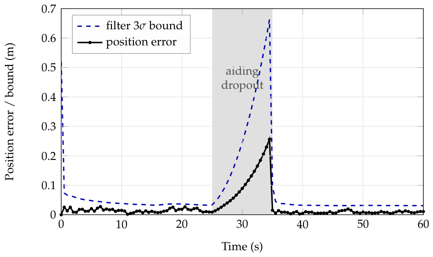
Figure 5.
Monte Carlo NEES of the ESKF on synthetic data ( runs of the Figure 4 scenario with initial errors and IMU biases drawn from ; aiding dropout shaded). Top: run-averaged NEES of the full 15-D error state for the shipped filter () and with the reset Jacobian, which overlap; dashed lines bound the two-sided 95% interval. Bottom: 3-D blocks of the shipped filter against the 3-dof interval. The full-state NEES lies above the interval at most epochs and never below it; attitude is the most overconfident block, position and velocity exceed the interval mainly during and after the dropout, and both bias blocks stay inside it.
Figure 5.
Monte Carlo NEES of the ESKF on synthetic data ( runs of the Figure 4 scenario with initial errors and IMU biases drawn from ; aiding dropout shaded). Top: run-averaged NEES of the full 15-D error state for the shipped filter () and with the reset Jacobian, which overlap; dashed lines bound the two-sided 95% interval. Bottom: 3-D blocks of the shipped filter against the 3-dof interval. The full-state NEES lies above the interval at most epochs and never below it; attitude is the most overconfident block, position and velocity exceed the interval mainly during and after the dropout, and both bias blocks stay inside it.
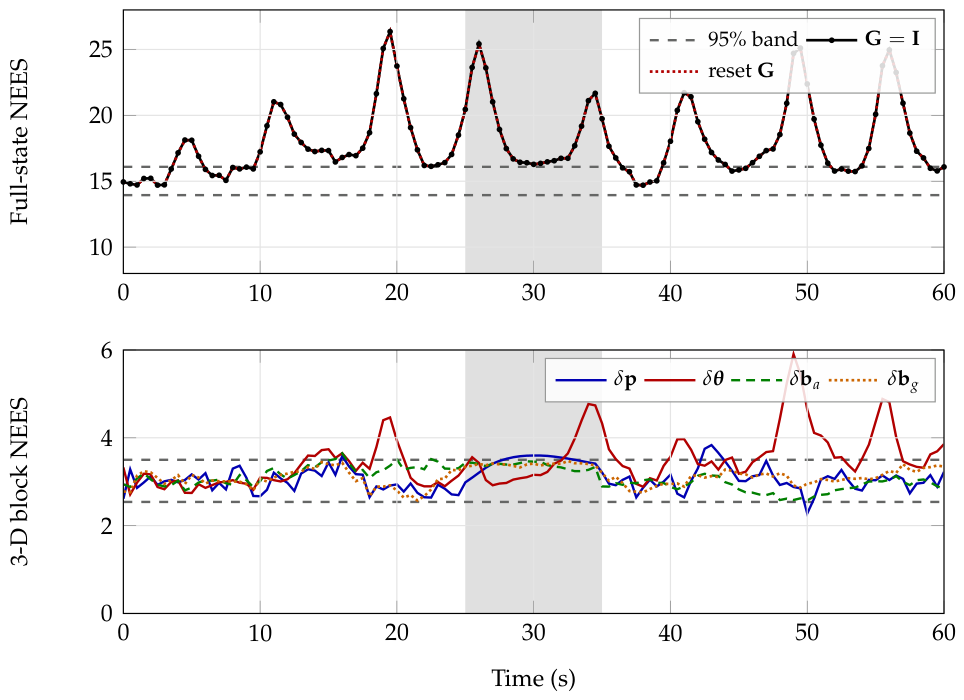
Table 3.
laser2d steady-state tracking error on synthetic data ( s, 110 logged samples per seed at 2 Hz). Columns are computed from data/mcl_tracking.csv; the last two rows pool the three seeds as mean ± std of the per-seed values and as statistics over all 330 samples.
Table 3.
laser2d steady-state tracking error on synthetic data ( s, 110 logged samples per seed at 2 Hz). Columns are computed from data/mcl_tracking.csv; the last two rows pool the three seeds as mean ± std of the per-seed values and as statistics over all 330 samples.
| Seed | Mean pos. err. (m) | Max pos. err. (m) | Mean yaw err. (rad) | Max yaw err. (rad) |
|---|---|---|---|---|
| 101 | 0.113 | 0.269 | 0.034 | 0.120 |
| 202 | 0.100 | 0.257 | 0.030 | 0.105 |
| 303 | 0.102 | 0.288 | 0.033 | 0.184 |
| Per-seed | – | – | ||
| Pooled (330 samples) | 0.105 | 0.29 | 0.032 | 0.18 |
Table 4.
Relocalization and fusion results on synthetic data. Left: branch-and-bound over kidnapped-robot queries (data/bbs_relocalization.csv); percentiles use linear interpolation; latency is single-threaded wall-clock on the machine that produced the committed CSV. Right: ESKF position error by window relative to the 10 s aiding dropout (data/eskf_track.csv, logged at 2 Hz).
Table 4.
Relocalization and fusion results on synthetic data. Left: branch-and-bound over kidnapped-robot queries (data/bbs_relocalization.csv); percentiles use linear interpolation; latency is single-threaded wall-clock on the machine that produced the committed CSV. Right: ESKF position error by window relative to the 10 s aiding dropout (data/eskf_track.csv, logged at 2 Hz).
| BBS relocalization | ESKF fusion | |||
|---|---|---|---|---|
| Success (pos. m, yaw ) | 97 / 100 | RMSE before dropout ( s) | 0.016 m | |
| Median / p95 position error | 0.037 / 0.072 m | RMSE during dropout ( s) | 0.125 m | |
| Median / p95 yaw error | 0.48∘ / 1.74∘ | Peak error (at s) | 0.256 m | |
| Accepted at / false accepts | 78 / 0 | RMSE after dropout ( s) | 0.009 m | |
| Median score fraction | 0.632 | Peak bound (at s) | 0.663 m | |
| Median latency (min, p95) | 37.65 ms (8.77, 106.07) | Samples with error | 0 / 121 | |
Table 5.
Relocalization on large synthetic maps: v0.1 window versus map-sized window. Warehouse-like maps with repeated shelf rows at 0.1 m/cell; kidnapped poses stratified by whether they lie inside (in) or outside (out) the set the v0.1 node searched ( m to m about the map center); the 20 m map lies entirely inside it. Each cell reads v0.1 / current matcher on identical scans (U beam clutter). Success: position error m and yaw error ; accepted: ; false accept: accepted but not a success. Latency is the single-threaded median (data/bbs_largemap.csv, generated by experiments/bbs_largemap.cpp).
Table 5.
Relocalization on large synthetic maps: v0.1 window versus map-sized window. Warehouse-like maps with repeated shelf rows at 0.1 m/cell; kidnapped poses stratified by whether they lie inside (in) or outside (out) the set the v0.1 node searched ( m to m about the map center); the 20 m map lies entirely inside it. Each cell reads v0.1 / current matcher on identical scans (U beam clutter). Success: position error m and yaw error ; accepted: ; false accept: accepted but not a success. Latency is the single-threaded median (data/bbs_largemap.csv, generated by experiments/bbs_largemap.cpp).
| Map | Poses | N | Success | Accepted | False accepts | Median latency (ms) |
|---|---|---|---|---|---|---|
| 20 m | in | 60 | 60 / 60 | 50 / 50 | 0 / 0 | 29 / 29 |
| 40 m | in | 60 | 53 / 54 | 57 / 57 | 4 / 3 | 74 / 127 |
| 40 m | out | 60 | 2 / 50 | 41 / 48 | 39 / 3 | 150 / 220 |
| 80 m | in | 60 | 51 / 53 | 54 / 55 | 6 / 4 | 391 / 1547 |
| 80 m | out | 60 | 0 / 41 | 51 / 52 | 51 / 11 | 334 / 1484 |
Table 6.
Single-scan acceptance versus multi-scan verification on the maps, poses and first scans of Table 5. Each cell reads single scan / verified ( modes, scans, Section 3.5); the robot drives 0.3 m steps with noisy odometry between scans. Correct: accepted and within 0.5 m and of the truth at the committed scan; false accepts with the 95% Wilson interval of their rate in percent; ambiguous: verification ended without a hypothesis holding 0.9 of the normalized evidence score. Latency: median over the whole decision, measured with three concurrent workers (data/bbs_verify.csv, experiments/bbs_verify.cpp).
Table 6.
Single-scan acceptance versus multi-scan verification on the maps, poses and first scans of Table 5. Each cell reads single scan / verified ( modes, scans, Section 3.5); the robot drives 0.3 m steps with noisy odometry between scans. Correct: accepted and within 0.5 m and of the truth at the committed scan; false accepts with the 95% Wilson interval of their rate in percent; ambiguous: verification ended without a hypothesis holding 0.9 of the normalized evidence score. Latency: median over the whole decision, measured with three concurrent workers (data/bbs_verify.csv, experiments/bbs_verify.cpp).
| Map | Poses | N | Correct | False accepts [95% CI, %] | Ambiguous | Median latency (ms) |
|---|---|---|---|---|---|---|
| 20 m | in | 60 | 50 / 49 | 0 [0.0, 6.0] / 0 [0.0, 6.0] | 0 | 35 / 127 |
| 40 m | in | 60 | 54 / 54 | 3 [1.7, 13.7] / 0 [0.0, 6.0] | 1 | 129 / 261 |
| 40 m | out | 60 | 45 / 45 | 3 [1.7, 13.7] / 0 [0.0, 6.0] | 1 | 238 / 399 |
| 80 m | in | 60 | 51 / 50 | 4 [2.6, 15.9] / 0 [0.0, 6.0] | 2 | 1351 / 1752 |
| 80 m | out | 60 | 41 / 44 | 11 [10.6, 29.9] / 1 [0.3, 8.9] | 6 | 1093 / 1526 |
| 40 + 80 m | all | 240 | 191 / 193 | 21 [5.8, 13.0] / 1 [0.1, 2.3] | 10 | 535 / 762 |
Table 8.
Ablation of the BBS acceptance threshold (Equation (11)), recomputed post hoc from the score fractions in data/bbs_relocalization.csv; no search is re-run. “Rejected correct” counts successful matches that the threshold would discard. The shipped default is .
Table 8.
Ablation of the BBS acceptance threshold (Equation (11)), recomputed post hoc from the score fractions in data/bbs_relocalization.csv; no search is re-run. “Rejected correct” counts successful matches that the threshold would discard. The shipped default is .
| 0.20 | 0.25 | 0.30 | 0.35 | 0.40 | 0.45 | 0.50 | 0.60 | |
|---|---|---|---|---|---|---|---|---|
| Accepted | 100 | 98 | 94 | 84 | 78 | 73 | 67 | 54 |
| False accepts | 3 | 2 | 0 | 0 | 0 | 0 | 0 | 0 |
| Rejected correct | 0 | 1 | 3 | 13 | 19 | 24 | 30 | 43 |
Table 9.
Ablation by clutter level. The 100 BBS queries of Figure 3 split into thirds of the clutter range by the per-query clutter_frac column; success as in Table 4, acceptance at .
| Clutter probability | Queries | Success | Accepted | Median pos. err. (m) | Median score fraction |
|---|---|---|---|---|---|
| 37 | 37 | 37 | 0.040 | 0.831 | |
| 30 | 30 | 30 | 0.032 | 0.624 | |
| 33 | 30 | 11 | 0.037 | 0.353 |
Disclaimer/Publisher’s Note: The statements, opinions and data contained in all publications are solely those of the individual author(s) and contributor(s) and not of MDPI and/or the editor(s). MDPI and/or the editor(s) disclaim responsibility for any injury to people or property resulting from any ideas, methods, instructions or products referred to in the content. |
© 2026 by the authors. Licensee MDPI, Basel, Switzerland. This article is an open access article distributed under the terms and conditions of the Creative Commons Attribution (CC BY) license (http://creativecommons.org/licenses/by/4.0/).
Copyright: This open access article is published under a Creative Commons CC BY 4.0 license, which permit the free download, distribution, and reuse, provided that the author and preprint are cited in any reuse.