What Aggregate Scores Hide: Group Baselines for Fine-Grained Claims

1. Introduction

Aggregate prediction scores are often used as evidence of fine-grained structure; we examine what selected scores establish independently of the other evidence in the original studies. Examples include linear probes that recover the coordinates of places from language-model activations (Gurnee & Tegmark, 2024) and the ideology of politicians (Kim, Evans & Schein, 2025); the words of tweets that predict county heart-disease mortality (Eichstaedt et al., 2015); and LLM judges agree with human preferences about as often as humans agree with each other (Zheng et al., 2023). We chose these as well-known illustrations, not as a sample, and do not estimate how common the pattern is; Supplement E lists the analysed cases, including those in which the headline passes. In each case the target is grouped – places by country, politicians by party, counties by state, votes by which models wrote the answers – and a predictor that knows only the group may reach the score. We ask two questions of such headlines: how much of the score does knowing only the group give, and what does the representation add below it?

Our main worked example is the space and time probes of Gurnee & Tegmark, who read their scores as evidence for linear representations of space and time. Barenholtz (2026) obtains substantial spatial and weaker temporal recoverability from static co-occurrence embeddings, showing that linear recoverability alone is not specific to contextual model representations. Both papers contain evidence beyond aggregate scores; our reanalysis focuses on what the aggregate probe scores establish about prediction below specified groupings.

The group explanation is not new. Gurnee & Tegmark themselves note that a probe could place each place at its country’s centroid, and hold out whole countries, states and centuries to test it. On their standard split, however, a predictor that places each test location at its country’s training centroid scores R² = .962, above the published .881 [C338], and predicting each held-out block at its parent region’s centroid beats their held-out errors (Supplement C) [C342].

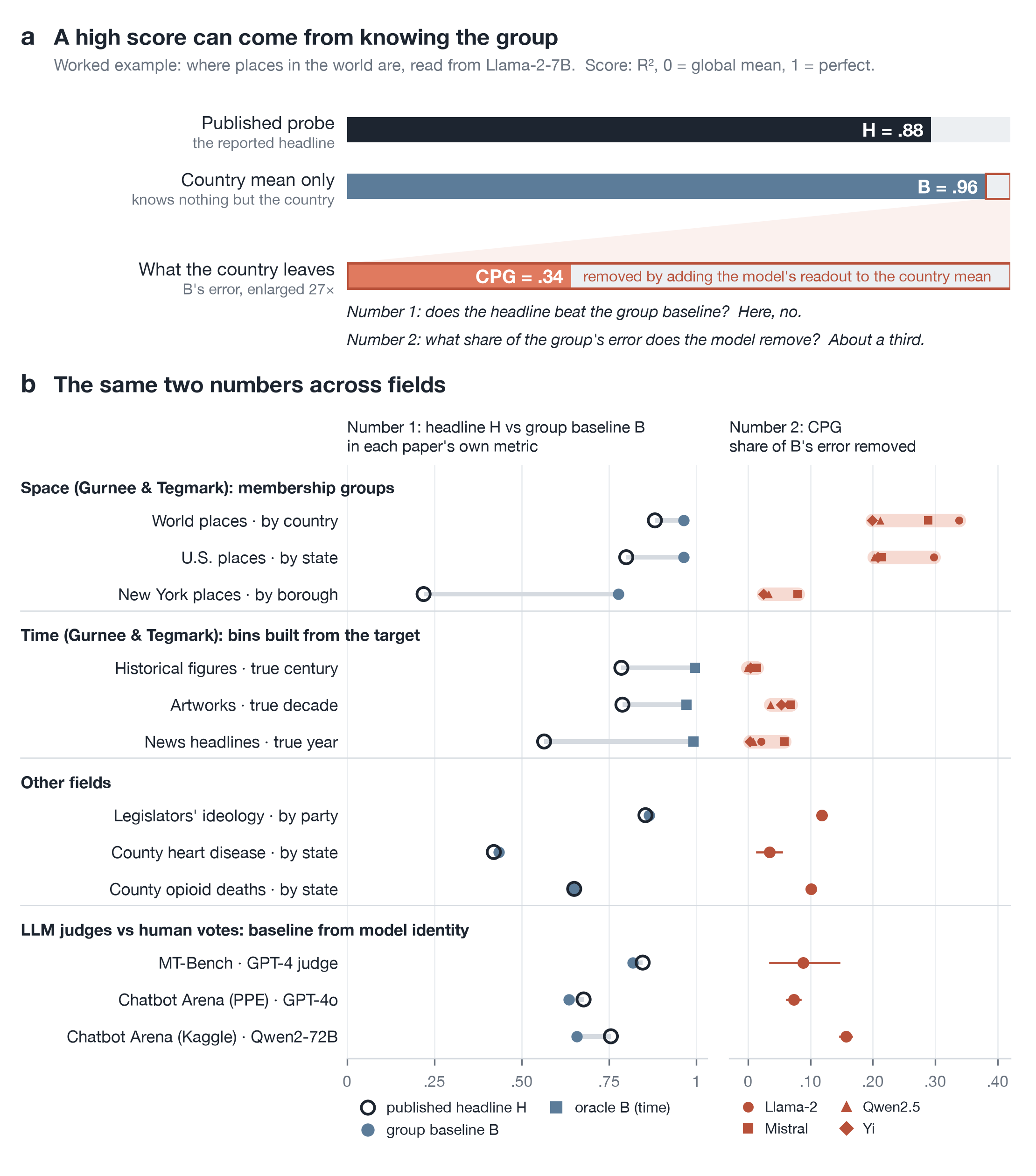
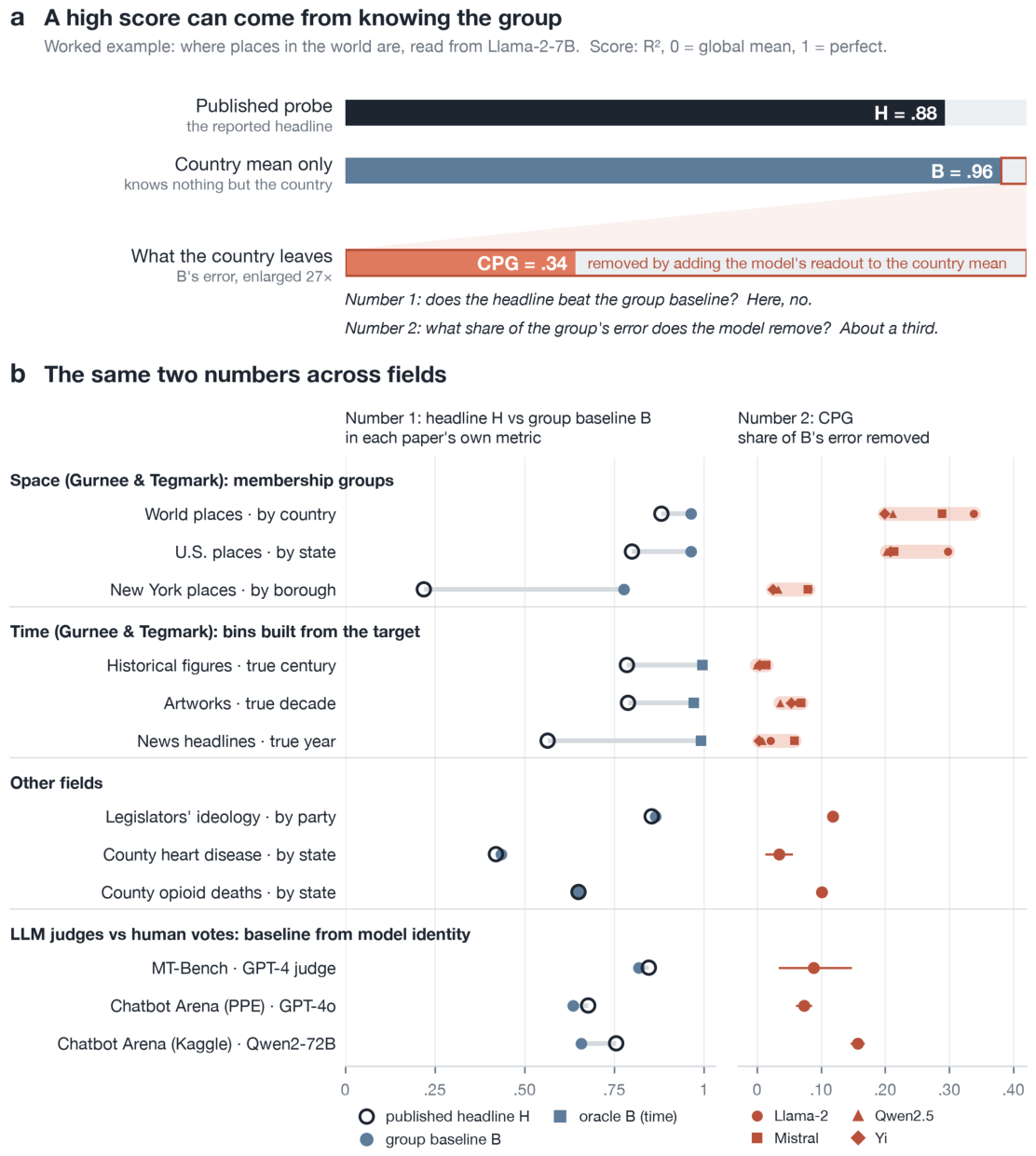
The group baseline is an information and resolution diagnostic, not a competitor with the same inputs: it asks whether a headline could have been attained from the group alone, not whether the original probe attained it that way. We separate three questions that aggregate scores blend: could group structure alone attain the headline (the group baseline); does the representation improve prediction beyond the group, and where (the conditional predictive gain and its within-group part); and how much conditional predictive performance is already accessible from static name representations (a static-embedding comparison). Figure 1 shows the first two for every matched case. We make four contributions.

• An instrument. A training-only group baseline scored against each published headline in the paper’s metric and split, paired with a conditional predictive gain that carries intervals, a withingroup permutation null and an exact cell decomposition (Section 2; a small tool implements both).
• What lies below the category in language models. Beyond country and state means, residual readouts from four 6-7B models reduce the remaining coordinate error by 20-34%, almost entirely within groups; one level down in USA, the saved readouts’ gain over state means is accounted for by differences between county cells rather than useful variation within counties; below the century, decade and year the gains are small. For a fourth model, the CPG point estimates satisfied thresholds frozen before evaluation in all five datasets; with whole countries resampled, theWorld interval reaches zero (Section 3.3).
• Matched and external static comparisons. On the same pipeline, each model’s input layer gains much less than its hidden layer within states and less within countries; a static co-occurrence embedding, on a different pipeline, also gains much less; in time all gains are small (Section 3.4).
• The same diagnostic in other applications. In LLM-as-judge validation, on retained non-tie votes, a predictor that knows only which models wrote the answers, and how often humans preferred each on other questions, agrees with human votes 2.8-9.7 percentage points less often than the judges (Section 4). Party alone matches a probe of political ideology in language-model activations, and state alone matches a famous Twitter prediction of county heart-disease mortality; the second number then shows ideology within party and a small additional predictive gain from the released Twitter topic features beyond state means (Section 5). In a baseline-only comparison, satellite-image predictions exceed their county-mean baselines (Section 5; unaudited).

Our contribution is not a new statistic. Asking what a representation makes predictable beyond a baseline is conditional probing (Hewitt et al., 2021), following control tasks (Hewitt & Liang, 2019); the normalized between-group variance is the squared correlation ratio; and for squared error CPG is the held-out increment in R² over a group baseline, normalized by the baseline’s unexplained share (applied per coordinate here), an out-of-sample analogue of the hierarchical increment in R² (Cohen et al., 2003); it is conceptually related to the conditional usable information of Hewitt et al., which builds on V-information (Xu et al., 2020), but is not an estimate of it. Gurnee & Tegmark themselves raised the group alternative; Brown & Coyne (2018) criticised the Twitter result but compared regions only through a north-south split of dictionary correlations, not through a state baseline in the paper’s metric; and Stephan et al. (2025) show that judges favour stronger candidate models. We add a provenance-tracked protocol that sets a held-out group baseline against specific published numbers in their own metric and split, with the gain beyond it and its within-group part, and reanalyse published claims across fields.

2. Two Numbers

Units i have a target y_i and a group g(i). A membership group is an externally specified category available at prediction time (country, state, party, the pair of models that wrote two answers). A resolution oracle is built from the target itself (century, decade, year); it asks how much of a headline survives once the coarse value is known, and is labelled as such.

Group baseline B. Predict each evaluation unit by the mean of y over training units of its group (global training mean if the group is absent from training), and score it with the paper’s own metric on the evaluation rows. For vote collections without a training split, the baseline is cross-fitted by excluding the entire evaluated question (Section 4). Section 4 applies the same logic with a domain-specific cross-fitted reduced model that uses only the two model identities (a model-identity baseline); it is not literally the group mean, and a calibration-half pair-majority baseline is reported beside it (Supplement G).

Conditional predictive gain. Let r be the reduced predictor (the group predictor) and p the full predictor, which adds the representation; both are fit on training data only and scored on the same held-out rows. Then

$$\begin{array}{c}\mathrm{CPG}={\displaystyle \frac{\mathrm{SSE}\left(r\right)-\mathrm{SSE}\left(p\right)}{\mathrm{SSE}\left(r\right)}}.\end{array}$$

For coordinates we compute CPG per axis and average. CPG can be negative. An improvement over estimated group means can include better estimation of the means themselves, so we split each predictor’s error over evaluation cells c (group x fold) into a cell-mean term M and a within-cell term W:

$$\begin{array}{c}M\left(p\right)=\sum _c{n}_c{({\overline{y}}_c-{\overline{p}}_c)}^2,W\left(p\right)=\sum _c\sum _{i\in c}{\left[(y_i-{\overline{y}}_c)-(p_i-{\overline{p}}_c)\right]}^2,\mathrm{SSE}\left(p\right)=M\left(p\right)+W\left(p\right),\\ \mathrm{CPG}=\underset{\mathrm{cell}-\mathrm{mean}\mathrm{part}}{\underbrace{{\displaystyle \frac{M\left(r\right)-M\left(p\right)}{\mathrm{SSE}\left(r\right)}}}}+\underset{\mathrm{within}-\mathrm{cell}\mathrm{part}}{\underbrace{{\displaystyle \frac{W\left(r\right)-W\left(p\right)}{\mathrm{SSE}\left(r\right)}}}}.\end{array}$$

The cell-mean part credits better group-level averages; the within-cell part credits predicting how units deviate from their own cell’s mean, and it is not a rank statistic. A cell with a single unit contributes nothing to the within-cell part. A predictor can order units correctly within a cell and still have a negative within-cell part if its deviations are too large or too small: the part rewards calibrated deviations, not ranks. When the published headline uses a correlation, B is compared with H in that metric, while CPG is reported separately under squared loss as a nested-prediction diagnostic; it is not a decomposition of the published correlation. The centring on evaluation cells only describes prediction errors; it is not used to fit any predictor. Example: for a single target, B = .964 and CPG = .30 mean that the full predictor removes 30% of the remaining 3.6% error, giving R² = .975.

Estimators. The additive readout adds to the group centroid a ridge readout trained on the residual y - c(g); the joint fit also centres the features on group means (Frisch-Waugh-Lovell) and can recover within-group signal that the additive readout misses. Penalties are tuned by cross-validation that recomputes group means inside each split. In the county cases of Section 5 the additive readout is fitted to residuals cross-fitted over five inner folds, with state means recomputed in each, and its penalty is chosen by leave-one-out cross-validation on that fixed residual series; the joint fit centres outcomes and features on the outer-training state means and chooses its penalty by exact leave-one-out cross-validation that accounts for the unpenalised group intercepts. Neither refits the whole two-stage pipeline inside each penalty-selection split. The additive specification follows the declared residual-readout protocol. Because it residualizes the target but not the representation, we report the cell decomposition and, where available, the joint fit as a complementary estimator; where the joint fit was run, both are reported (Section 3.1 and Section 3.2, Supplement C), and they can differ substantially (Art .065 against .129 for Llama-2-7B; ideology .118 against .269).

Uncertainty. Intervals are conditional evaluation-set bootstrap intervals: 95% percentiles of 2,000 paired bootstrap resamples (10,000 for the question-clustered judge intervals of Table ) of evaluation rows and, where the rows span at least 20 groups, of whole groups. Both condition on the fitted predictors and leave out the variability of representation extraction, fitting and penalty selection. A within-group permutation null shuffles the predictions inside each group and tests only the within-cell component. An interval that includes zero is not evidence that information is absent.

Tool. A short Python module scores features or aligned total predictions, with joint fitting available on the feature route; it reports B, CPG with both intervals, the decomposition, the permutation null and a resolution profile, and reproduces the audited Llama-2-7B, ideology and county values used here (Supplement J). The research harness and case-specific scripts provide the provenance checks listed in Supplement A.

Use of AI tools. Generative AI agents wrote and ran the analysis code and drafted the text under the author’s direction, and a separate AI agent audited the protocols and replayed reported numbers; the Declarations give the full statement, with model versions and the division of decisions.

Provenance identifiers. Bracketed identifiers point to frozen analyses (D, I) and to audits by the separate AI auditor (C), which in some cases replayed the reported numbers from the saved outputs with its own code and in others reviewed protocols and wording; Supplement A maps each reported statistic to its source, and the audit records are released with the code.

3. Below the Category in Language Models

We use the released World, USA and NYC place datasets and the historical-figure, artwork and headline datasets of Gurnee & Tegmark, with their split, prompts and probe layer (their layer 20 of 32, our hidden_states[21]; for Qwen2.5-7B, which has 28 layers, this layer is not depth-matched). The models are Llama-2-7B (Touvron et al., 2023), Mistral-7B (Jiang et al., 2023), Qwen2.5-7B (Qwen Team, 2024) and Yi-6B (01.AI, 2024). Groups are country, state and borough for space, and century of death, decade of release and year of publication for time.

Table 1. Published headline H (Llama-2-7B), group baseline B (rows as in the note below the table), and CPG of the additive readout beyond the group, per model. H and B are total scores in the paper’s metric; CPG is the share of the error left by B that the readout removes, a different scale (in World and USA, CPG .20-.34 is an increase in total R² of .008-.013; Section 2 gives a worked example). Bracketed: 95% row-bootstrap interval; where the rows span at least 20 groups, the 95% group-bootstrap interval follows after the semicolon (both conditional on the fitted predictors).

dataset (group)	H	B	Llama-2-7B	Mistral-7B	Qwen2.5-7B	Yi-6B (frozen test)
Membership groups
World (country)	.881	.963	.338 [.299, .385; .101, .471]	.289 [.253, .339; .106, .416]	.212 [.187, .241; .026, .314]	.199 [.172, .229; -.000, .311]
USA (state)	.799	.964	.298 [.280, .317; .108, .403]	.214 [.203, .226; .107, .300]	.202 [.184, .220; .021, .307]	.208 [.191, .226; .054, .296]
NYC (borough)	.219	.777	.080 [.061, .101]	.079 [.069, .089]	.033 [.015, .052]	.025 [.007, .042]
Resolution oracles (built from the target)
Historical figures (century)	.785	.996	.007 [.002, .012; -.013, .035]	.014 [.009, .019; -.009, .044]	-.001 [-.007, .006; -.025, .035]	.004 [-.001, .010; -.010, .024]
Art (decade)	.788	.972	.065 [.051, .078]	.069 [.058, .080]	.036 [.026, .046]	.053 [.043, .063]
Headlines (year)	.564	.991	.021 [.013, .030]	.058 [.050, .065]	.008 [.003, .013]	.003 [-.001, .007]

Rows: H is the published score on all test rows; B and CPG use the test rows whose group appears in training (World 7,903 of 7,917, with B = .962 on all rows; NYC 3,960 of 3,967). Sources: Llama-2-7B D071 [C463, C468]; Mistral and Qwen D070 [C429, C444]; Yi-6B D090 [C480, C485]; group intervals for Llama-2-7B D093 and for Yi-6B D097 [unaudited]. Our Llama-2-7B probes reproduce the published scores (World .881, USA .798, NYC .219; Historical .785, Headlines .564) except Art, .771 against the published .788, a reproduction discrepancy of .017; on the rows of B, the reproduced probe scores .881 in World (equal to four decimals) and .214 in NYC [D102; C506].

Table 1. Published headline H (Llama-2-7B), group baseline B (rows as in the note below the table), and CPG of the additive readout beyond the group, per model. H and B are total scores in the paper’s metric; CPG is the share of the error left by B that the readout removes, a different scale (in World and USA, CPG .20-.34 is an increase in total R² of .008-.013; Section 2 gives a worked example). Bracketed: 95% row-bootstrap interval; where the rows span at least 20 groups, the 95% group-bootstrap interval follows after the semicolon (both conditional on the fitted predictors).

dataset (group)	H	B	Llama-2-7B	Mistral-7B	Qwen2.5-7B	Yi-6B (frozen test)
Membership groups
World (country)	.881	.963	.338 [.299, .385; .101, .471]	.289 [.253, .339; .106, .416]	.212 [.187, .241; .026, .314]	.199 [.172, .229; -.000, .311]
USA (state)	.799	.964	.298 [.280, .317; .108, .403]	.214 [.203, .226; .107, .300]	.202 [.184, .220; .021, .307]	.208 [.191, .226; .054, .296]
NYC (borough)	.219	.777	.080 [.061, .101]	.079 [.069, .089]	.033 [.015, .052]	.025 [.007, .042]
Resolution oracles (built from the target)
Historical figures (century)	.785	.996	.007 [.002, .012; -.013, .035]	.014 [.009, .019; -.009, .044]	-.001 [-.007, .006; -.025, .035]	.004 [-.001, .010; -.010, .024]
Art (decade)	.788	.972	.065 [.051, .078]	.069 [.058, .080]	.036 [.026, .046]	.053 [.043, .063]
Headlines (year)	.564	.991	.021 [.013, .030]	.058 [.050, .065]	.008 [.003, .013]	.003 [-.001, .007]

Rows: H is the published score on all test rows; B and CPG use the test rows whose group appears in training (World 7,903 of 7,917, with B = .962 on all rows; NYC 3,960 of 3,967). Sources: Llama-2-7B D071 [C463, C468]; Mistral and Qwen D070 [C429, C444]; Yi-6B D090 [C480, C485]; group intervals for Llama-2-7B D093 and for Yi-6B D097 [unaudited]. Our Llama-2-7B probes reproduce the published scores (World .881, USA .798, NYC .219; Historical .785, Headlines .564) except Art, .771 against the published .788, a reproduction discrepancy of .017; on the rows of B, the reproduced probe scores .881 in World (equal to four decimals) and .214 in NYC [D102; C506].

Table 2. Judge agreement H, model-identity baseline B, their gap, the relative disagreement reduction (RDR) and the nested Brier CPG on retained non-tie votes with valid verdicts (Kaggle: order-consistent verdicts only). Brackets: 95% percentile resampling intervals over whole question identifiers (MT-Bench), normalized prompt groups (Kaggle) or votes (PPE, one vote per identifier), with predictions held fixed; vote-resampling intervals are in Supplement G.

data (judge)	votes (question groups)	H	B	gap H - B	RDR, 0-1 loss	nested Brier CPG
MT-Bench experts (GPT-4)	1,723 (80)	.846	.818	+.028 [+.009, +.051]	.156 [.054, .259]	+.088 [+.035, +.146]
PPE Chatbot Arena (GPT-4o)	9,186 (9,186)	.677	.635	+.042 [+.031, +.054]	.116 [.086, .146]	+.073 [+.062, +.084]
Kaggle Chatbot Arena (Qwen2-72B)	27,605 (25,640)	.755	.658	+.097 [+.090, +.103]	.283 [.266, .298]	+.157 [+.147, +.166]

Sources: I149c, I151, I154b of the companion analysis, audited in its C386, C389, C396; nested Brier CPG I170b (companion audit C414; post hoc); intervals I185 (companion audit C464).

Table 2. Judge agreement H, model-identity baseline B, their gap, the relative disagreement reduction (RDR) and the nested Brier CPG on retained non-tie votes with valid verdicts (Kaggle: order-consistent verdicts only). Brackets: 95% percentile resampling intervals over whole question identifiers (MT-Bench), normalized prompt groups (Kaggle) or votes (PPE, one vote per identifier), with predictions held fixed; vote-resampling intervals are in Supplement G.

data (judge)	votes (question groups)	H	B	gap H - B	RDR, 0-1 loss	nested Brier CPG
MT-Bench experts (GPT-4)	1,723 (80)	.846	.818	+.028 [+.009, +.051]	.156 [.054, .259]	+.088 [+.035, +.146]
PPE Chatbot Arena (GPT-4o)	9,186 (9,186)	.677	.635	+.042 [+.031, +.054]	.116 [.086, .146]	+.073 [+.062, +.084]
Kaggle Chatbot Arena (Qwen2-72B)	27,605 (25,640)	.755	.658	+.097 [+.090, +.103]	.283 [.266, .298]	+.157 [+.147, +.166]

Sources: I149c, I151, I154b of the companion analysis, audited in its C386, C389, C396; nested Brier CPG I170b (companion audit C414; post hoc); intervals I185 (companion audit C464).

Table 3. CPG of the released Twitter topic features for county heart-disease mortality: share of the baseline’s squared error removed (additive readout; median over 20 random ten-fold partitions, and partition-0 intervals).

baseline	CPG (median; range over partitions)	partition-0 95% interval
state	.034 (.028-.038)	.014-.054 (counties); .011-.058 (whole states)
state plus the paper’s covariates	-.001 (-.008 to .003)	-.009 to .009 (counties); -.010 to .011 (whole states)

Sources: C429, C444, C419 (D070). On partition 0, about .030 of the state-baseline gain lies within state x fold cells; the median paired pooled-r increment beyond state plus covariates is .0006.

Table 3. CPG of the released Twitter topic features for county heart-disease mortality: share of the baseline’s squared error removed (additive readout; median over 20 random ten-fold partitions, and partition-0 intervals).

baseline	CPG (median; range over partitions)	partition-0 95% interval
state	.034 (.028-.038)	.014-.054 (counties); .011-.058 (whole states)
state plus the paper’s covariates	-.001 (-.008 to .003)	-.009 to .009 (counties); -.010 to .011 (whole states)

Sources: C429, C444, C419 (D070). On partition 0, about .030 of the state-baseline gain lies within state x fold cells; the median paired pooled-r increment beyond state plus covariates is .0006.

3.1. Space: A Consistent Conditional Gain Below Country and State Means

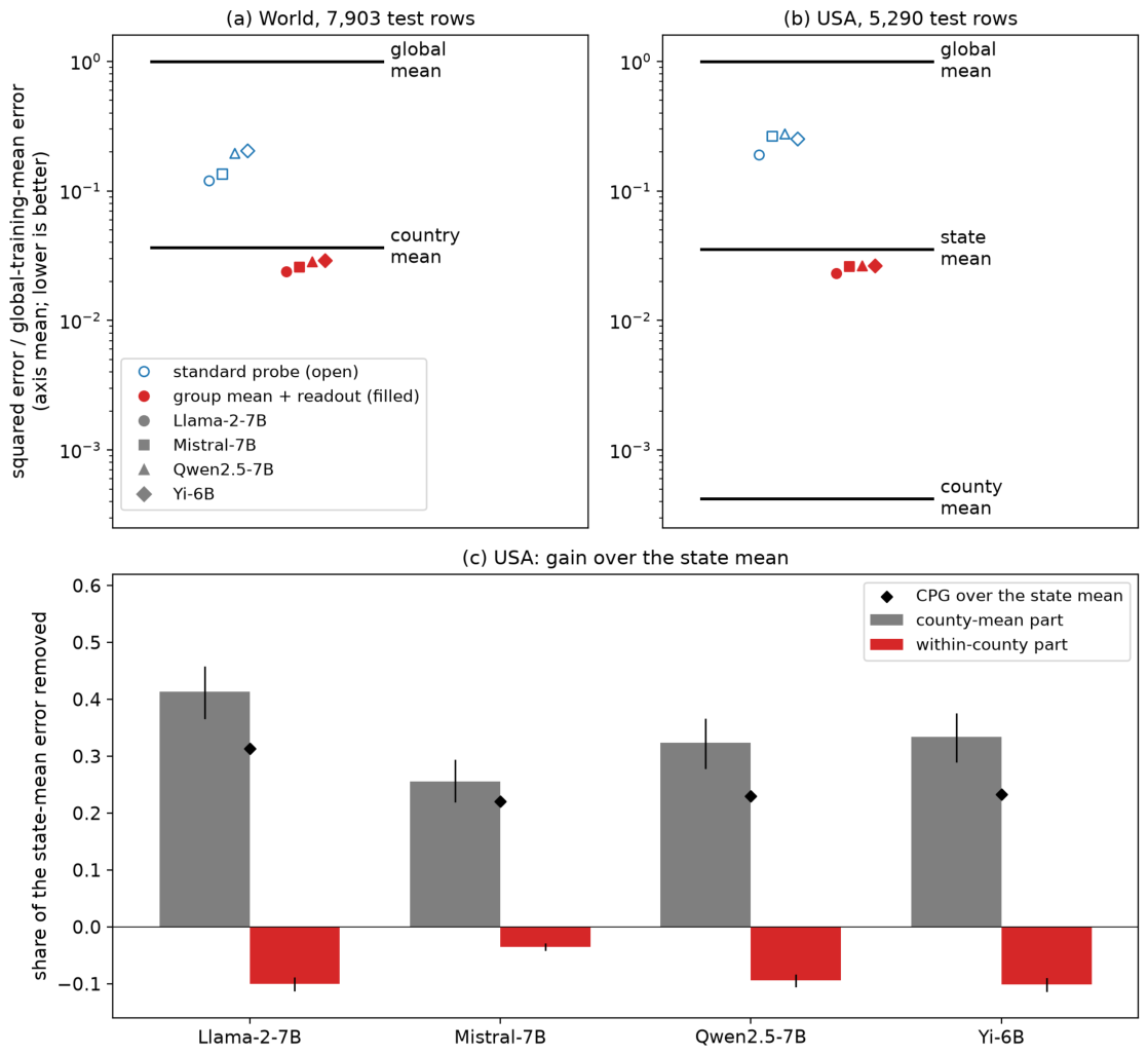
In every model and in both World and USA, B exceeds the published headline, yet residual readouts improve on the country or state mean: CPG .20-.34 (joint fit, run for Llama-2-7B and Yi-6B: .22-.37) [D071, D090], an increase in total R² of .008-.013, computed per axis [D102; C506]; resampling whole groups widens the intervals, to about zero for Yi-6B in World. The gain lies almost entirely within cells (cell-mean parts -.006 to -.017): the readouts’ improvement over the country or state mean is almost entirely attributable to prediction of group-centred coordinates. The standard total-coordinate probe tracks location within groups much more weakly than the residual readout from the same layer (within-group correlation .26 vs .60 in Mistral World) [C378, C398], so matching the aggregate headline does not imply equally strong within-group prediction by the fitted probe. The standard probe itself fits worse than the country means (.881 against .962): a single ridge map from activations to coordinates does not reach even the country-level geography, while the residual readout starts from it. Within boroughs the gain is small (.02-.08).

One level down: the county. What lies below the state could be a map or a finer category. County groups use the released county_fips field, which the upstream builder copies from SimpleMaps city, ZIP and county records; neither that builder nor our analysis infers the county from the released target coordinates. These geographic labels supply finer location information, but their baseline performance does not establish that a model encodes county identity. Counties are keyed by state and county code, because two training ZIP records carry a neighbouring state’s county code (Supplement C). On the 5,290 USA test rows whose state-county pair appears in training, spanning 1,595 evaluation cells, a county-mean baseline reaches R² .9996 against .965 for the state mean. Under this state-to-county decomposition, each saved readout’s positive net gain over state centroids comes from the county-mean component (.26-.41 against a total of .22-.31), while its within-county variation increases squared error (within-county part -.035 to -.101; whole-county resampling intervals exclude zero). The within-county evidence comes from the 4,565 rows in the 870 counties with more than one test row (725 counties hold a single row and contribute nothing to that term); restricted to the 3,093 rows in the 309 state-county cells with at least five test rows, the within-county part is -.047 to -.132. A prediction frozen before computing held in all four models; for Mistral and Qwen it followed an earlier look at within-county correlations, for Llama-2-7B and Yi-6B it was a prospective test of previously uninspected county endpoints [D102; reproduced C506]. This describes the saved readouts, not the models’ internal coding: it does not show that the models encode county identity, and it does not separate a finer category from a continuous but noisy map, since negative squared-error gain can coexist with positive within-county correlation. A shared linear recalibration of the saved predictions within counties, cross-fitted over ten folds of whole counties, did not yield a statistically resolved positive within-county gain. It is a per-axis affine recalibration with coefficients shared across counties, not a full two-dimensional linear recalibration. The procedure and the frozen threshold (gain over county means at most .01 in every model) were declared before computing [D104, D104b]; the observed gain over county means, as a share of the county-mean baseline’s error, is -.001 to .002 and its within-county part -.001 to .001, and all conditional 95% whole-county intervals include zero, with upper ends of .0041 for the total and .0034 for the within-county part (Supplement C.8) [reproduced C519]. This bounds this procedure, conditional on its fits, not the information in the models; a readout trained below the county was not run. On this USA subset, training-only county centroids outperform all four saved state-residual readouts.

Figure 2. Resolution profile. (a, b) Squared error divided by the error of the global training mean (mean over coordinates; log scale; lower is better) for group means (lines), standard total-coordinate probes (open markers) and the group mean plus residual readout (filled markers), one marker shape per model; USA uses the 5,290 test rows whose state-county cell appears in training. (c) Each USA readout’s CPG over the state mean (diamonds), split into county-mean and within-county parts, with 95% whole-county resampling intervals (2,000 draws, conditional on the fitted predictions). Panels a-b and c use different denominators. Sources: D103 [C508]; D102 [C506]; Figure C1 gives the per-case overview.

Figure 2. Resolution profile. (a, b) Squared error divided by the error of the global training mean (mean over coordinates; log scale; lower is better) for group means (lines), standard total-coordinate probes (open markers) and the group mean plus residual readout (filled markers), one marker shape per model; USA uses the 5,290 test rows whose state-county cell appears in training. (c) Each USA readout’s CPG over the state mean (diamonds), split into county-mean and within-county parts, with 95% whole-county resampling intervals (2,000 draws, conditional on the fitted predictions). Panels a-b and c use different denominators. Sources: D103 [C508]; D102 [C506]; Figure C1 gives the per-case overview.

3.2. Time: Small Conditional Gains Under the Primary Additive Readout

Under the primary additive readout, CPG below the century, decade and year is at most .07 in every model, largest for Art (.04-.07). The joint fit, run for Llama-2-7B and Yi-6B, gives up to .129 (Art), still below every World and USA value (.199-.369; Supplement C) [D071, D090]. The frozen readings are LOW in two of three datasets for three models and INTERMEDIATE for Mistral, sensitivity-limited rather than zero [C403, C416, C468]. The share of variance the baseline leaves (1 - B) is similar for World (3.7%), USA (3.6%) and Art (2.8%); this descriptive comparison does not rule out differences in target noise, difficulty or the membership-versus-oracle distinction.

3.3. A Pre-Specified Holdout-Model Replication

Before any run, we froze a numeric prediction for a model used in no earlier analysis, Yi-6B: if it passes the same reproduction gates, CPG exceeds .10 within countries and states and stays below .10 within centuries, decades and years [D090]. The jobs were the Llama-2-7B jobs with only the model swapped, and the strict parsers were unchanged except for a disclosed one-ulp tolerance [D090b]. The gates passed (World .797, USA .725; Historical .728, Art .751) and the CPG point estimates satisfied the frozen thresholds in all five datasets (.199, .208; .004, .053, .003; smallest point distance .047) [C480, C485]. This is a prespecified point-estimate replication on the existing datasets, not five statistically established inequalities: resampling whole countries widens the World interval to [-.000, .311], below the .10 threshold at its lower end, because a few countries carry most of the baseline error [D097; unaudited].

3.4. Is It Already in the Names?

On the same readout pipeline, each model’s own input layer (the token embeddings of the name, without context) gains .013-.017 within states, under a tenth of the hidden layer’s .20-.35, and about half of it within countries; a static GloVe embedding, on a different pipeline, also gains much less (Supplement H, Table H1) [D098b, D099; C490, C492].

4. The Same Comparison in AI Evaluation: LLM-as-Judge

LLM judges are validated by their agreement with human pairwise preferences (Zheng et al., 2023). A unit is one vote; its group is the identity of the two models that wrote the answers. The model-identity baseline predicts that the stronger model’s answer wins, with each model’s strength its human win rate on votes not involving the evaluated question. Because the strengths come from human votes in the same collection, the baseline uses no answer content but does use human-labelled calibration votes that a deployed judge does not see. On 0-1 loss we report the relative disagreement reduction RDR = 1 - (1 - H)/(1 - B), the net relative reduction in the baseline’s disagreement rate with human votes; the judge can also introduce new errors where the baseline was correct. Because the judge here replaces the baseline rather than adding to it, RDR is not a CPG in the sense of Section 2; the nested comparison below is.

In all three collections, B comes within about 3-10 percentage points of H: on the retained votes, a cross-fitted predictor using only model identities and human-derived strength estimates agrees with humans 2.8-9.7 percentage points less often than the judges, so aggregate judge-human agreement alone does not establish answer-specific discrimination. Calibrating the strengths on a disjoint half of the questions, so that no held-out EVAL-fold vote enters the predictor, leaves the mean gaps at 2.4, 4.9 and 9.9 points over 20 random half-splits (Supplement G) [companion I184, companion audit C449]. Stephan et al. (2025) already show that judges favour the stronger candidate model; the baseline puts that tendency in the agreement metric itself. The judges do add something: they reduce the baseline’s disagreement rate by 12-28% (RDR), and on a descriptive MT-Bench expert subset (1,598 ordered triads from 1,074 distinct votes), GPT-4 and a second expert have RDR point estimates of .207 and .171 (I149c, unaudited); this comparison does not establish statistical equivalence or show that either relies on model identity; and the CPG of the nested comparison, which adds the judge’s vote to a strength-based baseline, is +.088, +.073 and +.157 on Brier loss (Table ), of which the within model-pair x outer-fold cell parts are +.072, +.067 and +.124 (I170b, companion audit C414; post hoc).

Evaluation population. Retention differs, and every result in this section applies to the retained subset: MT-Bench keeps 1,723 of 2,668 expert votes (574 human ties and 371 tied or order-inconsistent judge verdicts removed), PPE 9,186 of 16,038 battles (5,822 human ties, then 1,030 missing judge verdicts among the remaining rows) and Kaggle 27,605 of 49,938 battles (15,641 human ties, 6,691 order-inconsistent verdicts, one judge tie); both predictors are scored on the same retained votes.

Uncertainty. MT-Bench has 80 questions (median 22 retained votes each); Kaggle’s 27,605 votes fall in 25,640 normalized prompt groups; PPE has a unique identifier per vote and no prompt text. The intervals in Table resample whole question identifiers for MT-Bench and normalized prompt groups for Kaggle; PPE’s use votes, so dependence from repeated underlying prompts cannot be assessed there. They hold predictions, fitted parameters, folds and retained-row masks fixed and do not propagate refitting or selection variability [companion I185; companion audit C464 reviewed the implementation and counts but did not independently replay the interval endpoints]. The nested comparison’s outer folds keep each observed question identifier (normalized prompt group on Kaggle) together. Supplement G gives the full protocol, a pair-majority baseline, strength-gap quintiles, a ground-truth test on GSM8K, the other judges and reward models, and the failed predictions.

5. The Same Diagnostic in Other Applications, and When the Headline Passes

Political ideology in language models. Kim, Evans & Schein (2025) report that a single attention head’s activations rank U.S. legislators by DW-NOMINATE ideology at Spearman .854. Party alone gives .864 on the same folds [C367]. Within party the activations still carry ideology. With the head chosen inside each training fold, they remove .118 of the party baseline’s squared error (.269 with the joint fit; unaudited); with the globally selected head, which can be optimistic, .127 [C429, C431]. The globally selected head’s predictions correlate with ideology at Spearman .41 among Democrats and .48 among Republicans, and nested head selection gives .35-.49 across three models [C367, C370, C440]. Kim et al. also test transfer to news outlets and interventions on generated text, which this comparison does not reassess (Supplement D).

County mortality from Twitter. Eichstaedt et al. (2015) report that Twitter language predicts county heart-disease mortality at r = .42, above ten demographic and health covariates (.36). Knowing only each county’s state reaches mean-fold r .435 under the same protocol [C388]. The released topic features then add little beyond state (Table 3). These are ecological associations on the released features, not reanalyses of the original models (Supplement D).

Opioid mortality. For opioid mortality from social-media language (Giorgi et al., 2023) the state reaches pooled r .648 against the published .65, and the topics remove .101 of the state baseline’s squared error [C400, C429].

When the headline passes. The same diagnostic also identifies cases in which the published predictor stays well above the group baseline. In a baseline-only comparison (unaudited), satellite-image predictions of tree cover, population density and night lights (Rolf et al., 2021) exceed county means by .20-.46 in R², and two sanity checks (Othello-GPT’s board state; protein stability with TAPE) fall far above their group baselines; elevation is the exception (Supplement E). In five rule-selected protein assays, a one-slope adjustment using language-model scores yields CPG .010-.169 within mutated sites; these results are provisional, because the data-integrity questions described in Supplement F are unresolved (unaudited).

6. Discussion and Recommendation

What the two numbers allow one to say. A headline that a group-only predictor reaches cannot, by itself, support a claim about finer structure, and showing that the baseline attains the score does not show that the original probe attained it by exploiting the group; it can still be the right number for a deployment that has the group. A positive CPG shows that the fitted procedure improves on the group predictor on these rows; its within-cell component quantifies how much of the error reduction comes from predicting group-centred target values, and it can be positive or negative. Neither number identifies a mechanism.

Relation to structured validation. Spatial and hierarchical cross-validation (Roberts et al., 2017; Ploton et al., 2020; Wadoux et al., 2021) addresses how well a predictor generalises under dependence; the group baseline asks a different question, how much of a reported score the grouping alone could attain, and the two are complementary.

Space, time and the text. Under the primary additive readout, the measured CPGs in World and USA exceeded those in each of the three time datasets for all four models. This describes the two set-ups and is not a finding about spatial versus temporal representation: space is grouped by membership and time by target-derived resolution oracles, so the comparison is not controlled. The membership baselines for space and target-derived resolution oracles for time already match or exceed the reported total scores, while static name representations also recover some below-group spatial variation, and the selected hidden layer yields much larger within-state conditional gain than the corresponding input embeddings. One level down, the saved USA readouts improve through between-county differences and not within counties (Section 3.1); whether a readout trained below the county would find position within counties needs the activations and is left open.

Limitations. One prompt set and one layer per model; intervals condition on fitted predictions; group intervals are wide where a few groups dominate the error; the time groups are resolution oracles; the static comparison uses a different readout pipeline; the judge baseline is a model-strength instance of a group-only predictor, calibrated on human votes from the same collection, though a disjoint-half calibration gives similar gaps (Supplement G); several analyses are post hoc and marked as such; the audits were performed by a separate AI agent, and no independent human replication has been made. Several follow-ups were not run: a continuous resolution profile over successively finer geographic cells (resolution oracles), errors in kilometres and years, a full two-dimensional recalibration within counties, and a fully nested tuning of the county pipelines, all from saved outputs; a readout trained below the county on the activations; a depth-matched layer for Qwen2.5-7B; and a sensitivity analysis of the judge results to the tie and consistency filters.

Recommendation. When a target has a salient grouping that could plausibly attain much of the reported predictive performance, report the group baseline in the paper’s metric, the conditional predictive gain with its within-group part and intervals, and a resolution profile of the baseline across grouping levels.

References

- AI. Yi: Open foundation models by 01.AI. arXiv 2024, arXiv:2403.04652. [Google Scholar]
- Aiken, E.; Rolf, E.; Blumenstock, J. Fairness and representation in satellite-based poverty maps: Evidence of urban-rural disparities and their impacts on downstream policy. IJCAI 2023 (AI for Social Good) 2023, arXiv:2305.01783. [Google Scholar] [CrossRef]
- Barenholtz, E. World properties without world models: Recovering spatial and temporal structure from co-occurrence statistics in static word embeddings. arXiv 2026, arXiv:2603.04317. [Google Scholar]
- Brown, N.J.L.; Coyne, J.C. Does Twitter language reliably predict heart disease? A commentary on Eichstaedt et al. (2015a). PeerJ 2018, 6, e5656. [Google Scholar] [CrossRef]
- Calderon, N.; Reichart, R.; Dror, R. The alternative annotator test for LLM-as-a-judge: How to statistically justify replacing human annotators with LLMs. Proc. ACL 2025 2025, arXiv:2501.10970. [Google Scholar] [CrossRef]
- Chi, G.; Fang, H.; Chatterjee, S.; Blumenstock, J.E. Microestimates of wealth for all low- and middle-income countries. PNAS 2022, 119(3), e2113658119. [Google Scholar] [CrossRef]
- Cohen, J.; Cohen, P.; West, S.G.; Aiken, L.S. Applied multiple regression/correlation analysis for the behavioral sciences, 3rd ed.; Lawrence Erlbaum Associates, 2003. [Google Scholar]
- Eichstaedt, J.C.; Schwartz, H.A.; Kern, M.L.; et al. Psychological language on Twitter predicts county-level heart disease mortality. Psychol. Sci. 2015, 26(2), 159–169. [Google Scholar] [CrossRef]
- Frick, E.; Li, T.; Chen, C.; Chiang, W.-L.; Angelopoulos, A.N.; Jiao, J.; Zhu, B.; Gonzalez, J.E.; Stoica, I. How to evaluate reward models for RLHF. arXiv 2024, arXiv:2410.14872. [Google Scholar]
- Frisch, R.; Waugh, F.V. Partial time regressions as compared with individual trends. Econometrica 1933, 1(4), 387–401. [Google Scholar] [CrossRef]
- Gera, A.; Boni, O.; Perlitz, Y.; Bar-Haim, R.; Eden, L.; Yehudai, A. JuStRank: Benchmarking LLM judges for system ranking. arXiv 2025, arXiv:2412.09569. [Google Scholar]
- Giorgi, S.; Yaden, D.B.; Eichstaedt, J.C.; Ungar, L.H.; Schwartz, H.A.; Kwarteng, A.; Curtis, B. Predicting U.S. county opioid poisoning mortality from multi-modal social media and psychological self-report data. Sci. Rep. 2023, 13, 9027. [Google Scholar] [CrossRef]
- Gurnee, W.; Tegmark, M. Language models represent space and time. ICLR 2024 2024, arXiv:2310.02207. [Google Scholar] [CrossRef]
- Haldar, R.; Hockenmaier, J. Rating Roulette: Self-inconsistency in LLM-as-a-judge frameworks. arXiv 2025, arXiv:2510.27106. [Google Scholar]
- Henikoff, S.; Henikoff, J.G. Amino acid substitution matrices from protein blocks. Proc. Natl. Acad. Sci. 1992, 89(22), 10915–10919. [Google Scholar] [CrossRef]
- Hewitt, J.; Liang, P. Designing and interpreting probes with control tasks. EMNLP 2019, 2019. [Google Scholar]
- Hewitt, J.; Ethayarajh, K.; Liang, P.; Manning, C.D. Conditional probing: Measuring usable information beyond a baseline. EMNLP 2021 2021. [Google Scholar] [CrossRef]
- Hou, C.; Liu, D.; Zafar, A.; Shen, Y. Understanding language model scaling on protein fitness prediction. bioRxiv 2025. [Google Scholar] [CrossRef]
- Hugging Face. Open LLM Leaderboard (v1). 2023. Available online: https://huggingface.co/spaces/open-llm-leaderboard-old/open_llm_leaderboard (accessed on 2 October 2026).
- Jean, N.; Burke, M.; Xie, M.; Davis, W.M.; Lobell, D.B.; Ermon, S. Combining satellite imagery and machine learning to predict poverty. Science 2016, 353(6301), 790–794. [Google Scholar] [CrossRef]
- Jiang, A.Q.; Sablayrolles, A.; et al. Mistral 7B. arXiv 2023, arXiv:2310.06825. [Google Scholar]
- Kapoor, S.; Narayanan, A. Leakage and the reproducibility crisis in machine-learning-based science. Patterns 2023, 4(9), 100804. [Google Scholar] [CrossRef]
- Kargi, B.; Salinas, D. From uncertain judgments to calibrated rankings: Conformal Elo estimation for LLM evaluation. arXiv 2026, arXiv:2606.13221. [Google Scholar]
- Kim, J.; Evans, J.; Schein, A. Linear representations of political perspective emerge in large language models. ICLR 2025 2025, arXiv:2503.02080. [Google Scholar] [CrossRef]
- Kim, S.; Kang, D.; Kwon, T.; Chae, H.; et al. Evaluating robustness of reward models for mathematical reasoning. arXiv 2024, arXiv:2410.01729. [Google Scholar]
- Lambert, N.; Pyatkin, V.; Morrison, J.; Miranda, L.J.; et al. RewardBench: Evaluating reward models for language modeling. arXiv 2024, arXiv:2403.13787. [Google Scholar]
- Li, K.; Hopkins, A.K.; Bau, D.; Viégas, F.; Pfister, H.; Wattenberg, M. Emergent world representations: Exploring a sequence model trained on a synthetic task. ICLR 2023, 2023. [Google Scholar]
- Liu, Y.; Yao, Z.; Min, R.; Cao, Y.; et al. RM-Bench: Benchmarking reward models of language models with subtlety and style. arXiv 2024, arXiv:2410.16184. [Google Scholar]
- Livesey, B.J.; Marsh, J.A. Updated benchmarking of variant effect predictors using deep mutational scanning. Mol. Syst. Biol. 2023, 19, e11474. [Google Scholar] [CrossRef]
- Lovell, M.C. Seasonal adjustment of economic time series and multiple regression analysis. J. Am. Stat. Assoc. 1963, 58(304), 993–1010. [Google Scholar] [CrossRef]
- Malik, S.; Pyatkin, V.; Land, S.; Morrison, J.; et al. RewardBench 2: Advancing reward model evaluation. arXiv 2025, arXiv:2506.01937. [Google Scholar]
- Marquet, C.; Heinzinger, M.; Olenyi, T.; Dallago, C.; Erckert, K.; et al. Embeddings from protein language models predict conservation and variant effects. Hum. Genet. 2021, 141, 1629–1647. [Google Scholar] [CrossRef]
- Meier, J.; Rao, R.; Verkuil, R.; Liu, J.; Sercu, T.; et al. Language models enable zero-shot prediction of the effects of mutations on protein function. bioRxiv 2021. [Google Scholar] [CrossRef]
- Méloux, M.; Dirupo, G.; Portet, F.; Peyrard, M. The dead salmons of AI interpretability. arXiv 2025, arXiv:2512.18792. [Google Scholar]
- Modell, A. Probing for representation manifolds in superposition. arXiv 2026, arXiv:2605.18537. [Google Scholar]
- Munro, D.; Singh, M. DeMaSk: A deep mutational scanning substitution matrix and its use for variant impact prediction. Bioinformatics 2020, 36, 5322–5329. [Google Scholar] [CrossRef]
- Nanda, N.; Lee, A.; Wattenberg, M. Emergent linear representations in world models of self-supervised sequence models. BlackboxNLP 2023 2023, arXiv:2309.00941. [Google Scholar] [CrossRef]
- Norman, J.D.; Rivera, M.U.; Hughes, D.A. Reliability without validity: A systematic, large-scale evaluation of LLM-as-a-judge models. arXiv 2026, arXiv:2606.19544. [Google Scholar]
- Notin, P.; Kollasch, A.W.; Ritter, D.; van Niekerk, L.; Paul, S.; et al. ProteinGym: Large-scale benchmarks for protein design and fitness prediction; bioRxiv, 2023. [Google Scholar] [CrossRef]
- Pearson, K. On the general theory of skew correlation and non-linear regression. In Drapers’ Company Research Memoirs, Biometric Series II. (correlation ratio, eta); 1905. [Google Scholar]
- Pennington, J.; Socher, R.; Manning, C.D. GloVe: Global vectors for word representation. Proc. EMNLP 2014, 2014, 1532–1543. [Google Scholar] [CrossRef]
- Ploton, P.; et al. Spatial validation reveals poor predictive performance of large-scale ecological mapping models. Nat. Commun. 2020, 11, 4540. [Google Scholar] [CrossRef]
- Qwen Team. Qwen2.5 technical report. arXiv 2024, arXiv:2412.15115. [Google Scholar]
- Rao, R.; et al. Evaluating protein transfer learning with TAPE. NeurIPS 2019. [Google Scholar] [CrossRef]
- Roberts, D.R.; et al. Cross-validation strategies for data with temporal, spatial, hierarchical, or phylogenetic structure. Ecography 2017, 40(8), 913–929. [Google Scholar] [CrossRef]
- Robinson, W.S. Ecological correlations and the behavior of individuals. Am. Sociol. Rev. 1950, 15(3), 351–357. [Google Scholar] [CrossRef]
- Rolf, E.; Proctor, J.; Carleton, T.; Bolliger, I.; Shankar, V.; Ishihara, M.; et al. A generalizable and accessible approach to machine learning with global satellite imagery. Nat. Commun. 2021, 12, 4392. [Google Scholar] [CrossRef]
- Stephan, A.; Zhu, D.; Aßenmacher, M.; Shen, X.; Roth, B. From calculation to adjudication: Examining LLM judges on mathematical reasoning tasks. Proc. GEM Workshop 2025 2025, arXiv:2409.04168. [Google Scholar] [CrossRef]
- Thakur, A.S.; Choudhary, K.; Ramayapally, V.S.; Vaidyanathan, S.; Hupkes, D. Judging the judges: Evaluating alignment and vulnerabilities in LLMs-as-judges. arXiv 2024, arXiv:2406.12624. [Google Scholar]
- Touvron, H.; Martin, L.; et al. Llama 2: Open foundation and fine-tuned chat models. arXiv 2023, arXiv:2307.09288. [Google Scholar]
- Vafa, K.; Chen, J.Y.; Rambachan, A.; Kleinberg, J.; Mullainathan, S. Evaluating the world model implicit in a generative model. arXiv 2024, arXiv:2406.03689. [Google Scholar]
- Vendrow, J.; Vendrow, E.; Beery, S.; Madry, A. Do large language model benchmarks test reliability? arXiv 2025, arXiv:2502.03461. [Google Scholar]
- Verhoeven, I.; Mishra, P.; Shutova, E. What do reward models memorize? arXiv 2026, arXiv:2607.24484. [Google Scholar]
- Vieira, L.C.; Lin, S.; Wilke, C.O. Intrinsic dataset features drive mutational effect prediction by protein language models. bioRxiv 2026. [Google Scholar] [CrossRef]
- Wadoux, A.M.J.-C.; Heuvelink, G.B.M.; de Bruin, S.; Brus, D.J. Spatial cross-validation is not the right way to evaluate map accuracy. Ecol. Model. 2021, 457, 109692. [Google Scholar] [CrossRef]
- Wu, Z.; Yasunaga, M.; Cohen, A.; Kim, Y.; et al. reWordBench: Benchmarking and improving the robustness of reward models with transformed inputs. arXiv 2025, arXiv:2503.11751. [Google Scholar]
- Xu, M.; et al. PEER: A comprehensive and multi-task benchmark for protein sequence understanding. In NeurIPS 2022 Datasets and Benchmarks; 2022. [Google Scholar]
- Xu, Y.; Zhao, S.; Song, J.; Stewart, R.; Ermon, S. A theory of usable information under computational constraints. ICLR 2020 2020, arXiv:2002.10689. [Google Scholar] [CrossRef]
- Yeh, C.; Perez, A.; Driscoll, A.; Azzari, G.; Tang, Z.; Lobell, D.; Ermon, S.; Burke, M. Using publicly available satellite imagery and deep learning to understand economic well-being in Africa. Nat. Commun. 2020, 11, 2583. [Google Scholar] [CrossRef]
- Zhang, G.; Badarayani, P.; Kumar, A.; Hasan, S.; Vesal, S. Can we trust LLM judges: A study of capability-dependent biases and multi-judge ensemble for bias calibration. arXiv 2026, arXiv:2609.12002. [Google Scholar]
- Zheng, L.; Chiang, W.-L.; Sheng, Y.; Zhuang, S.; Wu, Z.; Zhuang, Y.; Lin, Z.; Li, Z.; Li, D.; Xing, E.P.; et al. Judging LLM-as-a-judge with MT-Bench and Chatbot Arena. Adv. Neural Inf. Process. Syst. 2023, arXiv:2306.0568536. [Google Scholar]
Figure 1.
The two numbers. (a) Worked example (World places, Llama-2-7B): the published probe’s R2 (H), the R2 of training-set country means alone (B), and the conditional predictive gain (CPG) of the additive readout, the share of the country means’ squared error removed by adding the model’s readout to them; the bottom bar enlarges the error left by the country means to full width. (b) Every matched case in Sections 3-2-5: H (ring) and B (dot) in each paper’s own metric (R2 for space and time, Spearman correlation for ideology, Pearson r for the county outcomes, agreement rate for the judges), and CPG beyond B. For space and time, markers are the four models and the band their range (Table 1); the time baselines (squares) are resolution oracles built from the target, not membership groups. Judges: nested Brier CPG with question-clustered 95% intervals (Table). Heart disease: median over partitions with the partition-0 county interval (Table 3). Points are estimates; the intervals in Table 1 are wider when whole groups are resampled, and for Yi-6B in World the interval reaches zero (Section 3.3). Cases in which the headline stays well above the group baseline are in Section 5 and Supplement E. Where H and B coincide, the ring surrounds the dot.
Disclaimer/Publisher’s Note: The statements, opinions and data contained in all publications are solely those of the individual author(s) and contributor(s) and not of MDPI and/or the editor(s). MDPI and/or the editor(s) disclaim responsibility for any injury to people or property resulting from any ideas, methods, instructions or products referred to in the content. |
© 2026 by the author. Licensee MDPI, Basel, Switzerland. This article is an open access article distributed under the terms and conditions of the Creative Commons Attribution (CC BY) license.
Copyright: This open access article is published under a Creative Commons CC BY 4.0 license, which permit the free download, distribution, and reuse, provided that the author and preprint are cited in any reuse.