

Submitted:
02 October 2026
Posted:
06 October 2026
You are already at the latest version
Abstract
The Atlantic Equatorial Undercurrent (EUC) exhibits substantial variability in its vertical position, with implications for equatorial ocean dynamics and air–sea interactions. We investigate the oceanic and atmospheric conditions associated with anomalously deep and shallow EUC core-position events using monthly SODA oceanic and Twentieth Century Reanalysis (20CR) atmospheric data. The EUC core position is defined as the velocity-weighted vertical center of the eastward subsurface current, and events are identified from standardized position anomalies. We identify 95 independent deep and 84 shallow events, with mean core positions of 87.7 ± 4.1 and 58.1 ± 3.4 m, respectively. Despite this difference, mean maximum EUC velocities are similar (1.15 ± 0.14 and 1.13 ± 0.16 m s⁻¹). Composite analyses show contrasting reorganizations of the equatorial current system, vertical shear, temperature, SST, and SSH. Deep events exhibit stronger westward flow above the EUC, enhanced positive vertical shear, negative temperature, SST and SSH anomalies, and a steeper east–west thermocline slope than shallow events. SSH anomalies propagate eastward at approximately 1.2 m s⁻¹, consistent with Kelvin-wave-like signals. Contrasting wind-stress and sea-level-pressure anomalies further indicate distinct coupled ocean–atmosphere states rather than simple opposite phases of the same variability.
Keywords:
Atlantic Equatorial Undercurrent
; EUC core position
; equatorial ocean dynamics
; ocean–atmosphere coupling
; thermocline variability
; Kelvin waves
; tropical Atlantic
1. Introduction
The tropical Atlantic is characterized by strong interactions between oceanic circulation, upper-ocean thermal structure, atmospheric circulation, and equatorial wave dynamics. Within this coupled system, the Atlantic Equatorial Undercurrent (EUC) is a major pathway for the eastward transport of subsurface heat, mass, and biogeochemical properties. The EUC is a strong eastward-flowing subsurface current concentrated near the equator and generally embedded within the thermocline [1,2,3]. Its eastward extension toward the Gulf of Guinea contributes to equatorial upwelling and to the development and maintenance of the tropical Atlantic cold tongue [4,5,6,7].
The EUC exhibits significant variability on seasonal, interannual, and longer time scales. Its seasonal evolution is closely related to changes in equatorial wind stress, thermocline adjustment, and the propagation of equatorially trapped waves [6,8,9]. On longer time scales, EUC variability is also associated with tropical Atlantic climate variability, including Atlantic Niño events and related changes in equatorial thermocline structure [10,11,12].
Although changes in EUC velocity and transport have received considerable attention, the vertical position of the EUC velocity core represents a distinct aspect of EUC variability. The depth of the current maximum can vary substantially in response to changes in vertical shear, thermocline structure, stratification, and equatorial pressure gradients ([6,13,14]). Consequently, two periods characterized by a similar EUC velocity can nevertheless exhibit substantially different vertical configurations of the current.
This distinction is important because the vertical position of the EUC determines its relationship with the overlying South Equatorial Current (SEC), the thermocline, and the upper-ocean temperature structure.
A downward displacement of the EUC core increases its vertical separation from the surface westward-flowing currents and modifies the vertical shear structure of the upper ocean. Conversely, an upward displacement brings the EUC closer to the surface and alters the shear and hydrographic structure between the mixed layer and the thermocline. Because the EUC occupies the thermocline layer and the shear between the EUC and the overlying westward flow is an important component of upper-ocean mixing, changes in EUC core position can modify the dynamical coupling between subsurface circulation and the upper ocean [3,15]. These contrasting configurations may therefore be associated with different SST, sea-level, stratification, and atmospheric responses.
However, the two configurations have rarely been examined explicitly as opposite states of EUC core position. In particular, it remains unclear whether anomalously deep and anomalously shallow EUC-core positions are associated with mirror-like oceanic responses or instead represent dynamically asymmetric states. It is also unclear whether the atmospheric response differs between these two configurations and how equatorial wave propagation and upper-ocean shear contribute to their evolution.
The objective of this study is therefore not to identify EUC intensification events from anomalies in current velocity. Instead, we investigate episodes during which the EUC core is anomalously deep or anomalously shallow relative to its seasonal climatology. We then examine the oceanic and atmospheric anomalies associated with these two configurations and quantify their temporal evolution.
Specifically, the study addresses four questions:
- How does the vertical structure of the EUC differ between anomalously deep and anomalously shallow core-position events?
- What contrasting SST, subsurface temperature, SSH, thermocline, mixed-layer, and stratification anomalies accompany the two configurations?
- How do surface winds and vertical shear differ between deep-core and shallow-core events?
- To what extent can the observed asymmetry be interpreted in terms of equatorial wave propagation and coupled ocean–atmosphere adjustment?
By defining events from EUC-core position rather than velocity intensity, this framework isolates a structural mode of EUC variability. The associated changes in velocity, thermal structure, shear, sea level, and atmospheric circulation are subsequently treated as responses or diagnostics of the two contrasting EUC configurations.
The paper is structured as follows: Section 2 describes the SODA ocean reanalysis and Twentieth Century Reanalysis (20CR) atmospheric datasets, together with the calculation of the EUC core-position index (Iz), the identification of independent deep and shallow core-position events, and the composite analysis methodology. Section 3 presents the results, beginning with the climatological and seasonal characteristics of the EUC in the Gulf of Guinea and then examining the contrasting oceanic and atmospheric features associated with anomalously deep and shallow EUC core positions. Particular emphasis is placed on the distinction between EUC core position and maximum EUC velocity, followed by analyses of the contrasting thermal structure, vertical shear, sea surface height, equatorial wave propagation, surface wind stress, and sea-level pressure anomalies. Section 4 discusses the physical interpretation of the observed asymmetry between deep and shallow core-position configurations, with particular attention to the coupled oceanic and atmospheric processes, eastward-propagating equatorial Kelvin-wave-like signals, thermocline and mixed-layer adjustment, and SST–atmosphere coupling within the Lindzen–Nigam framework. Finally, Section 5 summarizes the main findings, discusses their implications for interpreting EUC variability, and identifies limitations and directions for future research.
2. Materials and Methods
2.1. Oceanic Datasets
The oceanic analysis uses monthly ocean reanalysis products to characterize the mean and anomalous three-dimensional structure of the EUC.
The primary long-term dataset is the Simple Ocean Data Assimilation product, SODA version 2.2.4, covering the period 1871–2008 SODA version 2.2.4 [16] available over 1871–2008, from which the 1900–2008 period was selected for this study. SODA provides monthly ocean velocity and hydrographic fields and is used to characterize the long-term climatological structure and variability of the EUC. The analysis considers the tropical Atlantic domain extending approximately from 60°W to 20°E and from 10°S to 30°N, with particular emphasis on the upper 200 m where the EUC and associated thermocline variability occur.
The oceanic variables considered include zonal velocity, meridional velocity, temperature, salinity, sea surface height, mixed-layer depth, and thermocline-related quantities. The Gulf of Guinea and the equatorial Atlantic are examined separately where appropriate to distinguish basin-scale propagation from the local response in the eastern basin.
2.2. Atmospheric Datasets
Atmospheric conditions associated with deep and shallow EUC-core positions are examined using the twentieth-century reanalysis (20CR).
The atmospheric variables include near-surface zonal and meridional winds, surface wind stress, sea-level pressure (SLP), and surface thermal variables where available [17]. The atmospheric analysis covers the tropical Atlantic domain, extending from approximately 60°W to 20°E and from 10°S to 30°N.
The 20CR product is particularly useful for extending the atmospheric analysis over the historical period corresponding to the SODA record. All atmospheric fields used for composites are converted to monthly anomalies relative to their corresponding monthly climatology before the event composites are calculated.
2.3. Climatology and Anomaly Calculation
The EUC core position and associated velocity metrics are calculated from the original monthly zonal velocity field. Seasonal anomalies are subsequently obtained by removing the corresponding monthly climatology from each derived time series or physical field.
For any variable , the monthly climatological mean is calculated for each calendar month over the baseline reference period:
where represents the total number of years in the dataset. The anomaly time series is then derived by subtracting the corresponding monthly climatology from the full field:
All standardized depth indices, velocities, stratification parameters, and atmospheric composite fields presented in this study are computed directly from these deseasonalized anomaly time series .
2.4. Identification of the EUC Core and Its Vertical Position
To accurately represent the vertical location of the EUC jet () and avoid numerical discretization noise associated with single-gridpoint maxima, the EUC core depth is defined using a velocity-weighted vertical center of mass (e.g., [6,18]).
First, at each longitude x and time step t, the meridionally averaged zonal velocity profile within the equatorial band (4°S–2°N) is extracted. The EUC core domain is restricted to the subsurface layer where eastward velocity satisfies a minimum current threshold , where isolates the core eastward flow of the EUC from background [6,18]. The vertical center-of-mass core depth is calculated as:
where integration limits span the vertical layer defined by . Concurrently, the maximum zonal velocity within the EUC core and the vertical core thickness are defined as:
where and denote the deepest and shallowest depths bounding the velocity core, respectively.
- a deep-core event corresponds to an anomalous downward displacement of the velocity-weighted EUC core position.
- a shallow-core event corresponds to an anomalous upward displacement of the velocity-weighted EUC core position.
Thus, the event classification does not imply that the EUC necessarily accelerates during either type of event.
The regional EUC-core position is subsequently averaged over the Gulf of Guinea sector, approximately 20°W–0°E, which provides the index used for event selection.
2.5. Gulf of Guinea Core Depth and Standardized Index
The regionally averaged core depth is derived by averaging specifically across the Gulf of Guinea (20°W–0°E):
The temporal climatological mean depth ( ) and standard deviation ( of are computed across the study period. The depth anomaly and the standardized EUC depth index are calculated as:
2.6. Definition of Deep and Shallow Core-Position Events
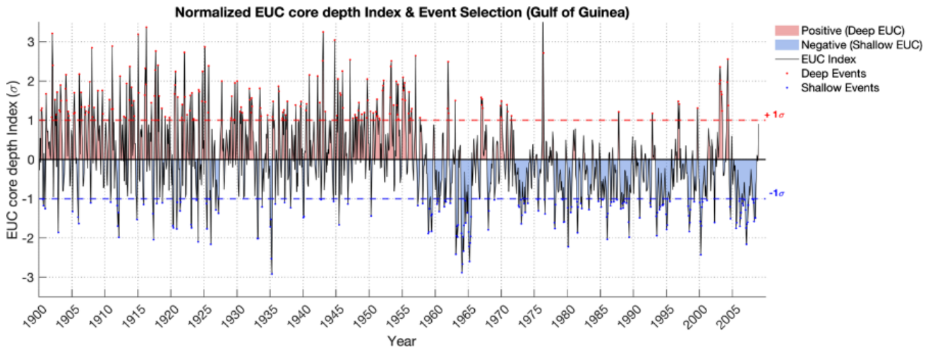
Using the standardized depth index , two distinct structural regimes are categorized based on a 1.0 standard deviation threshold:
- Deep EUC Events: Characterized by a downward displacement of the current core exceeding one standard deviation corresponding to
- Shallow EUC Events: Characterized by an upward displacement of the current core exceeding one standard deviation corresponding to
Figure 1.
Equatorial Undercurrent (EUC) core position index in the Gulf of Guinea (1900–2008) and composite event selection. Standardized monthly position anomalies (σ) of the EUC core (solid black line), deseasonalized relative to the 1900–2008 climatology. Shaded red and blue regions highlight anomalously deep (positive) and shallow (negative) position phases, respectively. Horizontal dashed lines mark the +1σ and −1σ selection thresholds used to isolate anomalous EUC position events for spatial composite analysis.
2.7. Event Independence
Because anomalous EUC positions can persist for several consecutive months, individual months satisfying the ±1σ criterion are not treated as independent events. Consecutive threshold-exceeding months are grouped into a single episode. The month corresponding to the largest absolute standardized depth anomaly within each episode is retained as the representative event month.
Two events are considered independent only when they are separated by at least two consecutive months that do not satisfy either event criterion. This minimum separation of two non-event months was imposed to reduce dependence between consecutive episodes while retaining sufficient events for composite analysis
This procedure prevents persistent episodes from artificially increasing the effective number of independent samples and avoids giving excessive weight to long-lived events.
The resulting sample of independent Deep and Shallow EUC events and their associated characteristics are summarized in Table 1.
The identified Deep and Shallow events (Table 1) exhibit a clear contrast in the vertical position of the Atlantic Equatorial Undercurrent (EUC) core. Deep events comprise 95 independent events, compared with 84 Shallow events, with similar mean durations of 1.98 ± 0.79 and 1.89 ± 1.37 months, respectively. The mean EUC core position is substantially deeper during Deep events (87.67 ± 4.07 m) than during Shallow events (58.10 ± 3.44 m), corresponding to mean position anomalies of +15.38 ± 4.07 m and −14.19 ± 3.44 m, respectively. In contrast, the mean maximum EUC velocity is very similar between the two categories (1.15 ± 0.14 m s⁻¹ for Deep and 1.13 ± 0.16 m s⁻¹ for Shallow events), indicating that the classification primarily distinguishes vertical displacements of the EUC core rather than changes in its maximum velocity. The mean thermocline depth is also comparable between the two categories, although slightly shallower during Deep events (69.07 ± 7.14 m) than during Shallow events (71.22 ± 5.84 m). Similarly, the mean mixed layer depth differs only marginally, with values of 25.38 ± 1.75 m and 24.86 ± 2.54 m for Deep and Shallow events, respectively. Overall, these statistics confirm that the two event categories are primarily distinguished by their contrasting EUC core positions, while their mean duration, maximum velocity, thermocline depth, and mixed layer depth remain broadly comparable.
2.8. Composite Analysis and Statistical Significance
To isolate the spatial and vertical physical signatures characteristic of deep versus shallow EUC events, composite anomalies of oceanographic and atmospheric variables ( are constructed. For each identified independent event peak ( ), anomalous fields are averaged across all N detected events for discrete time lags relative to the peak month ( months):
where represents the monthly anomaly field of variable , obtained by removing the long-term monthly climatology.
The statistical significance of the composite anomalies is evaluated using a non-parametric circular Monte Carlo permutation test (e.g., [19]). This method accounts for temporal autocorrelation and seasonal persistence in subsurface oceanographic and atmospheric fields without making strong parametric assumptions about the underlying distribution.
For each iteration (where =10000 permutations), the full anomaly time series is shifted circularly in time by a random offset , preserving the internal temporal correlation structure of the fields:
where T represents the total length of the time series, and is a uniformly distributed integer offset. Pseudo-composite fields are then recomputed using the original event peak dates .
The empirical p-value at each grid point is determined as the proportion of synthetic Monte Carlo iterations whose pseudo-composite value exceeds or equals the observed composite anomaly:
where is the indicator function. Regions where composite anomalies or composite differences are statistically significant at the 95% confidence level ( are highlighted in figures using stippling (black dots) or contour outlines.
2.9. Equatorial Wave Propagation
To investigate the role of equatorially trapped disturbances, longitude–time Hovmöller diagrams are constructed from equatorial SSH anomalies.
The Hovmöller fields are averaged over a narrow equatorial latitude band and plotted as a function of longitude and event-relative lag.
The propagation speed is estimated from the slope of coherent eastward-propagating sea surface height (SSH) anomalies in longitude–time space. Specifically, the propagation speed is obtained from the slope of a linear fit to the trajectory of the propagating SSH anomaly, with the longitude–time slope converted into velocity units (m s-1). The observed propagation speed is approximately 1.2 m s-1.
Because SSH phase speed alone does not uniquely identify the vertical baroclinic mode, we refer to these disturbances as eastward-propagating equatorial Kelvin-wave-like signals.
2.10. Vertical Shear
The magnitude of the vertical shear of the horizontal current is calculated as:
where (U) and (V) are the zonal and meridional components of the horizontal current, respectively, and (z) denotes depth.
The shear is examined together with the zonal velocity structure to determine how the vertical displacement of the EUC core relates to changes in the overlying and underlying currents.
3. Results
3.1. Climatological Structure and Seasonal Dynamics of the EUC in the Gulf of Guinea
The climatological EUC structure in the Gulf of Guinea exhibits pronounced seasonal variability in both velocity and vertical position. The monthly climatological evolution of the EUC velocity exhibits a bimodal seasonal cycle (Figure 2-a), with maxima during March–April and September–October. The maximum EUC zonal velocity reaches approximately 0.34 m s-1 whereas a relative reduction to approximately 0.28 m s-1 occurs during June–July (Figure 2-b). This seasonal modulation is consistent with the known influence of seasonal changes in equatorial wind stress and remotely forced equatorial ocean adjustment.
The vertical position of the EUC core also undergoes a pronounced seasonal migration. The core is relatively shallow during March–April, at approximately 60 m, whereas it reaches approximately 90 m during July (Figure 2-b). The seasonal deepening occurs at the same time as the strengthening of the westward South Equatorial Current in the upper 0–30 m (Figure 1-a).
The vertical structure therefore demonstrates that EUC velocity and EUC-core position are related but distinct quantities. In particular, the seasonal maximum in core velocity does not necessarily coincide with the deepest EUC configuration (Figure 2-c).
The spatial structure further shows that the EUC core generally becomes shallower toward the eastern basin. Core depths are approximately 80–100 m in the central Atlantic and approximately 40–60 m in the Gulf of Guinea. The current is strongest in the central Atlantic and progressively weakens toward the eastern boundary (Figure 2-d).
These climatological results establish the background state against which anomalously deep and shallow core-position events are identified. This seasonal phase difference between EUC intensity and core position provides an important basis for treating core position as a distinct diagnostic of EUC variability.
3.2. Contrasting Oceanic Responses to Deep and Shallow EUC-Core Positions
3.2.1. Composites of Temperature and Surface Wind Anomalies
The composite analysis reveals a strong thermal contrast between anomalously deep and anomalously shallow EUC-core configurations.
During deep-core events, negative SST anomalies develop over the eastern tropical Atlantic before and around the event peak. The cooling becomes particularly pronounced in the equatorial Atlantic and Gulf of Guinea near lag 0, where anomalies locally exceed approximately −0.8°C (Figure 3). This cooling phase is accompanied by enhanced south-easterly trade wind stress anomalies leading up to Lag 0. The co-occurrence of enhanced surface shear, subsurface cooling, and negative SST anomalies is consistent with enhanced vertical mixing and upwelling-favorable conditions.
The cooling is accompanied by enhanced southeasterly surface wind-stress anomalies before and around the event peak. The spatial and temporal coincidence of enhanced winds, surface cooling, and the downward displacement of the EUC is consistent with an active upwelling-favorable state in the eastern equatorial Atlantic.
The subsurface thermal structure provides further evidence for a strong cold anomaly. Negative temperature anomalies of approximately −1.5 to −2.0°C occur beneath the surface layer and extend toward the Gulf of Guinea (Figure 4). The combined surface and subsurface structure indicate that deep-core events are associated with a substantial redistribution of the upper-ocean thermal structure.
In contrast, the Shallow EUC regime (Figure 5) is characterized by positive SST anomalies across the equatorial Atlantic. Warm anomalies intensify rapidly from Lag -1, reaching peak values (> +0.8°C) at Lag 0 and Lag +1 centered over the Gulf of Guinea. Associated wind stress vectors show anomalous westerly/north-westerly flow along the equator, indicative of trade wind relaxation. Crucially, the warm SST anomaly exhibits temporal persistence, remaining statistically significant through Lag +4. The shoaled EUC core is consistent with reduced upward ventilation of subsurface cold water, trapping heat within the upper ocean and sustaining warm surface conditions.
The subsurface temperature structure features a pronounced shoaling of the EUC core (Figure 6), which shifts upward into the upper 20–60 m depth range in the eastern basin (15°W–5°E). This shoaled structure is associated with an intense positive subsurface temperature anomaly (> +1.5°C to +2.5°C) that propagates eastward from Lag -3 and peaks between Lag 0 and Lag +2 in the Gulf of Guinea. The shallow EUC configuration is associated with an altered and locally weakened thermocline temperature gradient, inhibiting cold-water upwelling and trapping warm thermal anomalies in the upper equatorial water column.
The two composites therefore exhibit a clear thermal asymmetry:
- deep-core configuration: colder surface and subsurface conditions;
- shallow-core configuration: warmer surface and subsurface conditions.
This contrast is consistent with a different relationship between the EUC core, thermocline structure, and the surface mixed layer.
3.2.2. Vertical Shear and EUC-Core Displacement
The latitude–depth composites reveal a strong contrast in the vertical shear structure associated with the two configurations.
In the Deep EUC regime (Figure 7), the westward-flowing South Equatorial Current (SEC) in the upper 0–30 m undergoes significant acceleration between Lag -1 and Lag +1. This surface intensification generates an intense positive vertical shear anomaly () in the intermediate layer (30–60 m) directly above the current core. The strong momentum transfer from the overlying SEC depresses the EUC jet core deeper into the thermocline layer, displacing its velocity maximum to depths of 70–90 m beneath the equator (1°S–1°N). Concurrently, both the mixed layer depth (MLD) and thermocline depth (THD) are deepened.
The spatial correspondence between enhanced upper-ocean westward flow, strong negative vertical shear, and the downward EUC displacement indicates that changes in the vertical velocity structure are an important component of the deep-core configuration.
Conversely, the Shallow EUC regime (Figure 8) exhibits a marked reorganization of the upper-ocean vertical velocity shear. The surface SEC weakens substantially, reducing the vertical shear in the upper ocean. This trade-wind relaxation allows the EUC core to shoal into the upper 30–60 m depth layer from Lag -1 to Lag +1. Under this configuration, a strong negative shear anomaly () develops above the shoaled core (20–50 m depth), while bottom-layer shear remains positive. This shoaling aligns the EUC core closely with the thermocline, establishing a direct dynamical link between subsurface momentum and surface ocean properties.
These relationships indicate that variations in the vertical position of the EUC are closely associated with the broader vertical structure of the equatorial current system.
3.2.3. Sea Surface Height and Equatorial Wave Propagation
The spatial evolution and longitude-time (Hovmöller) diagrams of Sea Surface Height (SSH) anomalies (Figure 9 and Figure 10) reveal an additional and particularly coherent asymmetry.
Under the Deep EUC regime (Figure 9), composite spatial maps show a prominent band of negative SSH anomalies (-2 to -5 cm) developing along the equatorial waveguide (5°S–5°N). The lower-right Hovmöller diagram demonstrates a coherent eastward propagation of these negative SSH anomalies from the central Atlantic (~35°W) towards the Gulf of Guinea (10°E) between Lag -3 and Lag +1. The estimated phase speed is approximately , which is broadly consistent with the phase speeds reported for second- and third-baroclinic-mode equatorial Kelvin waves in the Atlantic [20,21]. Given that phase speed alone does not uniquely identify the vertical baroclinic mode, we therefore interpret the observed disturbances as eastward-propagating equatorial Kelvin-wave-like signals.
The negative SSH signal is accompanied by a cold subsurface structure and enhanced surface cooling toward the eastern basin. Together, these features indicate an equatorial adjustment in which the vertical position of the thermocline and the EUC are strongly coupled.
The shallow-core composite exhibits the opposite SSH signature. Positive anomalies of approximately +3 to +5 cm extend along the equatorial Atlantic. The Hovmöller diagram indicates eastward propagation from the western-central basin toward the Gulf of Guinea, with a comparable phase speed of approximately at Lag -3 and reaching maximum amplitude in the Gulf of Guinea at Lag 0. The opposite signs of the SSH signals therefore suggest that deep and shallow EUC-core events are associated with opposite phases of an eastward-propagating equatorial disturbance.
3.3. Contrasting Atmospheric Responses
The atmospheric composites demonstrate that the two EUC-core configurations are also associated with contrasting sea-level-pressure and surface-wind anomalies (Figure 11 and Figure 12).
During deep-core events (Figure 11), a negative SLP anomaly occurs simultaneously with positive SST anomalies and develops over the central-western equatorial Atlantic several months before the event peak, reaching approximately −0.4 hPa in the strongest region. Around lag 0, this low-pressure anomaly weakens and is followed by a weak positive SLP anomaly over the eastern tropical Atlantic and Gulf of Guinea, generally on the order of +0.1 to +0.2 hPa.
The temporal evolution indicates that the atmospheric response is not spatially uniform. Instead, the pressure field evolves as the oceanic disturbance propagates toward the eastern boundary.
The positive SLP response following the cold SST anomaly is qualitatively consistent with a thermodynamic adjustment of the marine atmospheric boundary layer to surface cooling. Cooler surface conditions can increase near-surface air density and favor a relative pressure increase.
The shallow-core configuration exhibits a markedly different evolution. Positive SLP anomalies of approximately +0.3 to +0.5 hPa are present before the event peak, followed by the development of a negative pressure anomaly over the Gulf of Guinea and eastern equatorial Atlantic around lag 0 and into the positive-lag period.
The negative SLP anomaly reaches approximately −0.3 to −0.4 hPa and persists for several months. It occurs in association with positive SST anomalies and altered low-level wind convergence over the eastern basin.
The corresponding Hovmöller diagram confirms a sharp eastward propagation and intensification of this negative pressure anomaly between 0° and 10°E. This strong pressure fall reflects an efficient thermodynamic coupling (Lindzen–Nigam mechanism) forced by warm SST anomalies under a shallow thermocline/EUC configuration. Heating of the ABL dilates the surface air column, lowering local surface pressure (SLP<0). This sharp zonal and meridional pressure gradient actively forces strong surface wind convergence directly into the region of maximum warm SST anomalies over the eastern equatorial Atlantic and Gulf of Guinea.
This behavior is broadly consistent with an SST–atmosphere coupling mechanism, such as the pressure and surface-wind response to SST gradients described by [22]. However, the composites alone do not establish a one-way causal sequence. In particular, atmospheric pressure anomalies may also influence the oceanic evolution through their associated changes in surface wind stress.
4. Discussion
The composite analysis demonstrates a systematic asymmetry between periods characterized by anomalously deep and shallow EUC core positions. Importantly, this asymmetry is not limited to opposite-signed anomalies but involves distinct vertical configurations of the equatorial ocean and their associated thermal, dynamical, sea-level, and atmospheric states.
The deep-core configuration is characterized by a downward displacement of the EUC velocity-weighted core, enhanced westward SEC flow in the upper ocean, and stronger upper-layer vertical shear. It is also associated with colder subsurface waters, negative SST anomalies in the eastern equatorial Atlantic and Gulf of Guinea, and negative SSH anomalies. Conversely, the shallow-core configuration exhibits an upward displacement of the EUC core, weaker upper-ocean westward SEC flow, reduced upper-layer negative shear, warmer subsurface waters, and positive SST and SSH anomalies. These contrasting states therefore reflect different vertical structures of the equatorial circulation rather than simply opposite phases of the same surface signal.
The difference fields at Lag 0 provide further evidence of the dynamical connection between these contrasting configurations (Figure 13). In the Deep − Shallow composite, a pronounced negative zonal wind-stress difference (Δτx < −0.015 N m⁻²) extends across the western and central equatorial Atlantic (40°W–10°W, 5°S–5°N; Figure 13a). This anomaly is accompanied by an eastward-propagating negative SSH signal (Figure 13b), which extends from the central Atlantic toward the eastern Gulf of Guinea with an estimated phase speed of approximately 1.2 m s⁻¹. The propagation characteristics are consistent with an equatorial Kelvin-wave-like response, potentially involving higher baroclinic modes. The corresponding positive SSH signal in the Shallow − Deep sense indicates that the same propagating adjustment occurs with opposite phase in the shallow-core configuration.
The wave-related adjustment is accompanied by a pronounced modification of the upper-ocean structure. The Deep − Shallow difference in THD exceeds −25 m in parts of the Gulf of Guinea, indicating a shallower thermocline in the Deep state than in the Shallow state in these locations, while the mixed layer also becomes shallower by more than 20 m (Figure 13c,d). The equatorial longitude–depth section further reveals a strong negative subsurface temperature difference, locally exceeding −2.0 °C between approximately 40 and 80 m east of 15°W (Figure 13e). The THD contours emphasize the contrasting zonal structure of the thermocline: in the Deep state, the thermocline is deeper in the western basin and shoals progressively eastward, reaching depths of approximately 30 m between 15°W and 0°E, whereas in the Shallow state it is shallower in the west and deepens toward the eastern basin. The velocity-difference vectors additionally indicate enhanced anomalously enhanced upward motion in the Deep relative to the Shallow composite.
This subsurface adjustment is accompanied by pronounced surface cooling in the eastern equatorial Atlantic, where ΔSST reaches values below −1.0 °C in the equatorial cold-tongue region (10°W–5°E; Figure 13f). Taken together, the coherent differences in wind stress, SSH, thermocline depth, vertical velocity, subsurface temperature, and SST indicate that the Deep and Shallow EUC configurations are embedded within contrasting coupled ocean–atmosphere states. The eastward propagation of SSH anomalies provides an important organizing framework for these states, while the opposite signs of the propagating signals reflect their contrasting phases.
The coherent evolution of equatorial currents, thermocline structure, SSH, wind stress, SST, and atmospheric pressure indicates that Deep and Shallow events are embedded in distinct coupled ocean–atmosphere configurations. However, because the analysis is based on composite states, it does not establish a one-way causal relationship among these processes, nor does it demonstrate that EUC core position acts as an independent causal control on the coupled system.
A central implication is that EUC variability should not be characterized solely in terms of current intensity. The vertical position of the EUC core provides additional information about the vertical state of the equatorial circulation and about the coupling between subsurface ocean variability, the surface ocean, and the atmosphere. The distinction between Deep and Shallow core-position events consequently provides a complementary framework for interpreting equatorial Atlantic variability and its atmospheric expression.
5. Conclusions
This study examined the asymmetry between deep and shallow Atlantic Equatorial Undercurrent (EUC) core-position events and their associated oceanic and atmospheric conditions. Events were identified from anomalies in the vertical position of the EUC core, rather than from anomalies in EUC intensity. This distinction is important because the results show that substantial displacements of the EUC core can occur while the maximum EUC velocity remains of comparable magnitude between the two event categories. EUC vertical position therefore provides a complementary measure of EUC variability that is not simply a proxy for current strength.
Deep and shallow events are associated with markedly different three-dimensional oceanic states. Deep events are associated with a distinct zonal thermocline structure, characterized by a deeper thermocline in the western basin and progressive eastward shoaling, enhanced vertical shear in the upper ocean, colder subsurface waters, and negative SSH anomalies. These conditions are accompanied by negative SST anomalies and enhanced southeasterly wind-stress anomalies. Shallow events exhibit an opposite zonal thermocline structure, with a shallower thermocline in the west and progressive eastward deepening, weaker upper-ocean shear, warmer subsurface waters, positive SSH anomalies, and positive SST anomalies, together with anomalous westerly to northwesterly winds. The contrast therefore extends beyond the sign of the EUC position anomaly and involves coherent changes in the vertical structure of the equatorial upper ocean.
Both event types also exhibit eastward-propagating SSH anomalies along the equatorial Atlantic, with an estimated phase speed of approximately 1.2 m s⁻¹. This propagation is consistent with equatorial Kelvin-wave-like signals and suggests that large-scale equatorial dynamical adjustment is an important component of the evolution of EUC core-position anomalies. However, the phase speed alone does not establish a specific vertical baroclinic mode, nor does the composite analysis demonstrate a unique causal sequence between the propagating oceanic signal, EUC displacement, and surface atmospheric anomalies.
The associated SST, sea-level pressure, and wind-stress anomalies indicate that EUC core-position events occur as part of coupled ocean–atmosphere states. The spatial correspondence between SST, pressure, and wind anomalies is consistent with air–sea coupling over the tropical Atlantic, while the subsurface and SSH structures point to an important role for equatorial ocean dynamics. These relationships should nevertheless be interpreted as coupled associations rather than evidence for a one-way atmospheric or oceanic forcing mechanism.
Taken together, the results demonstrate that deep and shallow EUC core-position events represent distinct manifestations of equatorial Atlantic variability.Their differences in subsurface thermal structure, vertical shear, SSH, SST, and atmospheric conditions show that the vertical position of the EUC contains dynamical information that cannot be inferred from EUC intensity alone. Further investigation using direct Deep–Shallow statistical comparisons, independent EUC transport and velocity diagnostics, and a more explicit analysis of the vertical structure of the propagating signals will be required to establish the robustness and dynamical origin of the observed asymmetry
Acknowledgments
This work was supported by the International Joint Laboratory LMI-ECLAIRS-2 (Integrated Studies of Climate and Ocean in West Africa and Responses to Climate Change in Senegal). The authors acknowledge the National Oceanic and Atmospheric Administration (NOAA) and the Cooperative Institute for Research in Environmental Sciences (CIRES) for providing the Twentieth Century Reanalysis (20CR) datasets, and the SODA ocean reanalysis project for providing the oceanic datasets used in this study.
References
- Bourlès, B.; Gouriou, Y.; Chuchla, R. On the Circulation in the Upper Layer of the Western Equatorial Atlantic. J. Geophys. Res. Ocean. 1999, 104, 21151–21170. [Google Scholar] [CrossRef]
- Johns, W.E.; Townsend, T.L.; Fratantoni, D.M.; Wilson, W.D. On the Atlantic Equatorial Undercurrent Transport and Structure. J. Geophys. Res. Ocean. 2002, 107, 3167. [Google Scholar]
- Hazeleger, W.; de Vries, P. Subsurface Connections between the South Atlantic and the Equatorial Atlantic Ocean. J. Phys. Oceanogr. 2003, 33, 777–795. [Google Scholar]
- Weisberg, R.H.; Weingartner, T.J. Instability Waves in the Equatorial Atlantic Ocean. J. Phys. Oceanogr. 1988, 18, 1641–1657. [Google Scholar] [CrossRef]
- Voituriez, B. The Equatorial Upwelling in the Eastern Atlantic Ocean. Prog. Oceanogr. 1983, 12, 301–326. [Google Scholar]
- Kolodziejczyk, N.; Bourlès, B.; Marin, F.; Grelet, J.; Chuchla, R. Seasonal Variability of the Equatorial Undercurrent at 10°W as Inferred from Recent In Situ Observations. J. Geophys. Res. Ocean. 2009, 114, C06014. [Google Scholar] [CrossRef]
- Brandt, P.; Hahn, J.; Schmidtko, S.; Tuchen, F.P.; Kopte, R.; Kiko, R.; Bourlès, B.; Czeschel, R.; Dengler, M. Atlantic Equatorial Undercurrent Intensification Counteracts Warming-Induced Deoxygenation. Nat. Geosci. 2021, 14, 278–282. [Google Scholar] [CrossRef]
- Hisard, P.; Citeau, J.; Morlière, A. Le Courant de Lomonosov et l’Upwelling Équatorial du Golfe de Guinée. Cah. ORSTOM Sér. Océanogr. 1977, 15, 303–323. [Google Scholar]
- Weisberg, R.H.; Colin, C. Equatorial Atlantic Velocity and Temperature Observations during 1983–1984. J. Geophys. Res. Ocean. 1986, 91, 8417–8424. [Google Scholar]
- Zebiak, S.E. Air–Sea Interaction in the Equatorial Atlantic Region. J. Clim. 1993, 6, 1567–1586. [Google Scholar] [CrossRef]
- Carton, J.A.; Huang, B. Warm Events in the Tropical Atlantic. J. Phys. Oceanogr. 1994, 24, 888–903. [Google Scholar] [CrossRef]
- Lübbecke, J.F.; McPhaden, M.J. On the Asymmetry of Atlantic Niños and Niñas. J. Clim. 2012, 25, 2040–2051. [Google Scholar] [CrossRef]
- Colin, C.; Gallienne, F.; Chuchla, R. Hydrographic Conditions and Equatorial Wave Propagation in the Upper Layers of the Gulf of Guinea. Oceanol. Acta 1993, 16, 519–532. [Google Scholar]
- Brandt, P.; Funk, A.; Tantet, A.; Johns, W.E.; Fischer, J. The Equatorial Undercurrent in the Central Atlantic and Its Relation to Tropical Atlantic Variability. Clim. Dyn. 2014, 43, 2985–2997. [Google Scholar] [CrossRef]
- Jouanno, J.; Marin, F.; du Penhoat, Y.; Sheinbaum, J.; Molines, J.-M. Seasonal Heat Balance in the Upper 100 m of the Equatorial Atlantic Ocean. J. Geophys. Res. Ocean. 2011, 116, C09003. [Google Scholar] [CrossRef]
- Carton, J.A.; Giese, B.S. A Reanalysis of Ocean Climate and Variability with the Simple Ocean Data Assimilation (SODA). Mon. Weather Rev. 2008, 136, 2999–3017. [Google Scholar] [CrossRef]
- Compo, G.P.; Whitaker, J.S.; Sardeshmukh, P.D.; Matsui, N.; Allan, R.J.; Yin, X.; Gleason, B.E.; Vose, R.S.; Rutledge, G.; Bessemoulin, P.; et al. The Twentieth Century Reanalysis Project. Q. J. R. Meteorol. Soc. 2011, 137, 1–28. [Google Scholar] [CrossRef]
- Imbol Koungue, R.A.; Brandt, P. Impact of Intraseasonal Waves on Angolan Warm and Cold Events. J. Geophys. Res. Ocean. 2021, 126, e2020JC017088. [Google Scholar] [CrossRef]
- Wilks, D.S. Statistical Methods in the Atmospheric Sciences, 3rd ed.; Academic Press: Oxford, UK, 2011. [Google Scholar]
- Illig, S.; Dewitte, B.; Ayoub, N.; du Penhoat, Y.; Reverdin, G.; De Mey, P.; et al. Interannual Long Equatorial Waves in the Tropical Atlantic from a High-Resolution Ocean General Circulation Model Experiment in 1981–2000. J. Geophys. Res. Ocean. 2004, 109, C02022. [Google Scholar] [CrossRef]
- Polo, I.; Lazar, A.; Rodriguez-Fonseca, B.; Arnault, S. Oceanic Kelvin Waves and Tropical Atlantic Intraseasonal Variability: 1. Kelvin Wave Characterization. J. Geophys. Res. Ocean. 2008, 113, C07009. [Google Scholar] [CrossRef]
- Lindzen, R.S.; Nigam, S. On the Role of Sea Surface Temperature Gradients in Forcing Low-Level Winds and Convergence in the Tropics. J. Atmos. Sci. 1987, 44, 2418–2436. [Google Scholar] [CrossRef]
Figure 2.
(a) Monthly vertical-time section of zonal velocity (U, m s−1) in the upper 100 m. The overlaid black line with gray dots indicates the monthly depth of maximum EUC zonal velocity. (b) Seasonal cycle of the EUC core zonal velocity (Ucore , blue line, m s−1) and core depth (Zcore, red line, m) averaged over the Gulf of Guinea domain (20°W–0°E, 4°S–2°N). (c) Climatological monthly vertical profiles of zonal velocity (u, m s−1) in the upper 110 m. Open circles represent the depth and magnitude of the EUC core velocity peak (Umax ) for each month. (d) Spatial distribution of the annual mean EUC core velocity (shading, m s−1) overlaid with core depth isobaths (black contours, m). The dashed black line marks the equator (0°).
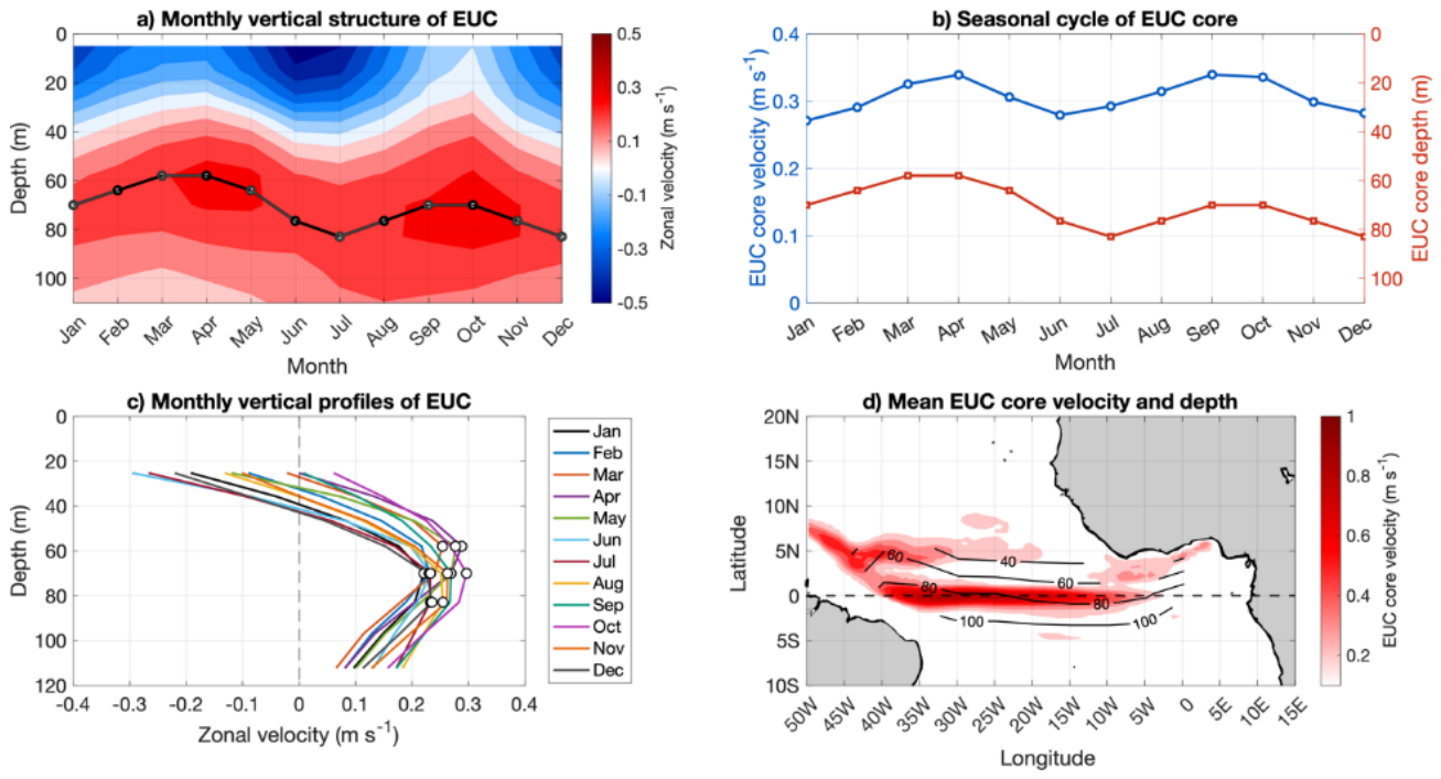
Figure 3.
Lead-lag composite maps spanning from Lag –5 months to Lag +4 months relative to deep EUC core position events (>+1σ). Colors represent composite SST anomalies (∘C, scale bar on the right). Bold vectors depict statistically significant surface wind stress anomalies (p<0.05). Grey stippling highlights ocean regions where SST anomalies are statistically significant at the 95% confidence level. Negative (positive) lags denote conditions leading up to (following) the peak deep EUC phase at Lag 0.
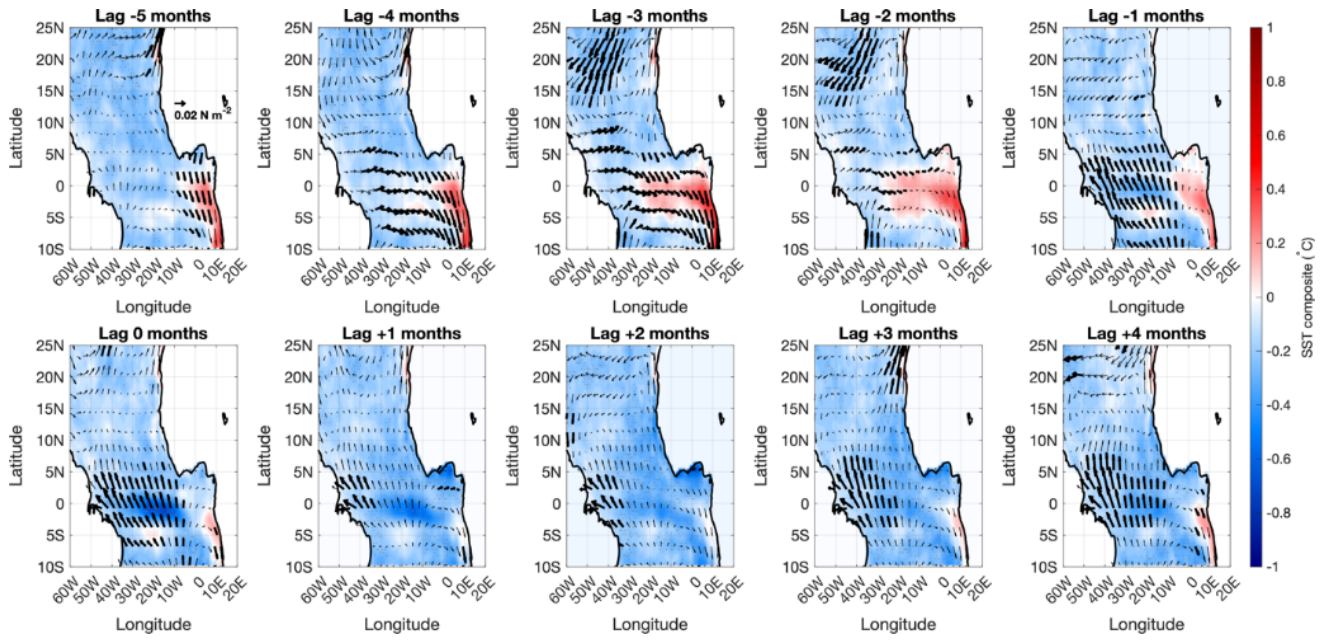
Figure 4.
Longitude-depth sections (0–110 m, averaged over the GG) from Lag –5 months to Lag +4 months relative to deep EUC core position events (>+1σ). Colors represent composite ocean temperature anomalies (∘C, scale bar on the right). Black vectors depict zonal velocity and vertical motion anomalies (u, w). The black dashed curve denotes the mixed layer depth (MLD), and the red dashed curve represents the thermocline depth (THD), defined as the level of maximum vertical temperature gradient. Grey stippling and Bold vectors highlight statistically significant temperature and wind stress anomalies at the 95% confidence level.
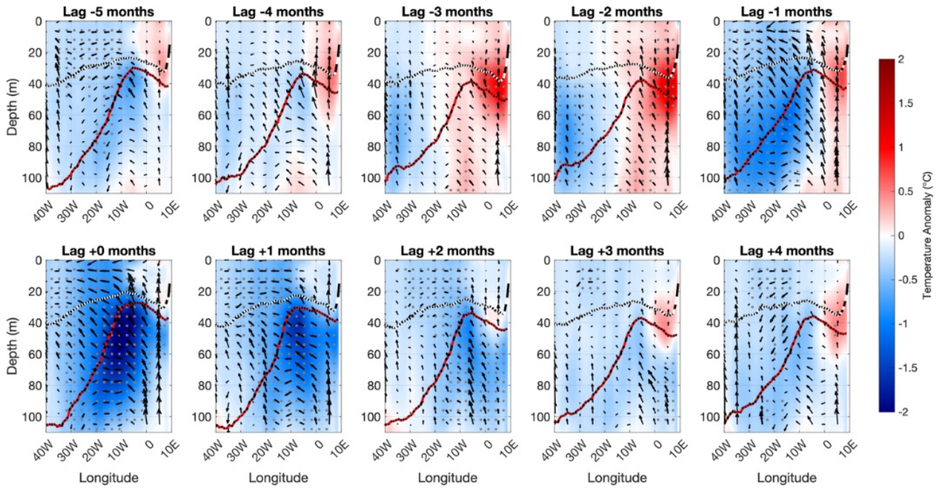
Figure 5.
Same as Figure 3, but for shallow EUC events (<−1σ). Lead-lag composite maps of SST anomalies (∘C, shading) and surface wind stress anomalies (vectors) from Lag –5 to +4 months relative to shallow EUC core position events. Bold vectors and grey stippling indicate statistical significance at the 95% confidence level.
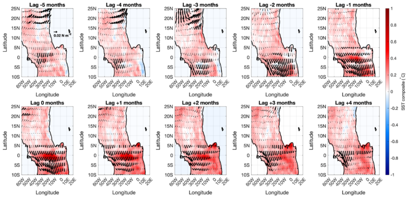
Figure 6.
Same as Figure 4, but for shallow EUC events.
Figure 6.
Same as Figure 4, but for shallow EUC events.
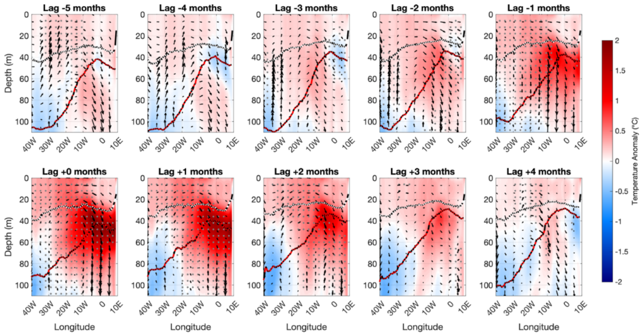
Figure 7.
Latitude-depth sections (4∘S–2°N, 0–110 m, averaged over the GG) from Lag –5 months to Lag +4 months relative to deep EUC core position events (±1σ). Colors represent composite vertical shear anomalies (s−1, scale bar on the right). Black contours depict the mean composite zonal velocity fields (U), where solid and dashed lines represent eastward and westward currents, respectively, highlighting the South Equatorial Current (SEC), Guinea Current (GC), and Equatorial Undercurrent (EUC). The thick dashed black and grey curves denote the composite mixed layer depth (MLD) and thermocline depth (THD), respectively.
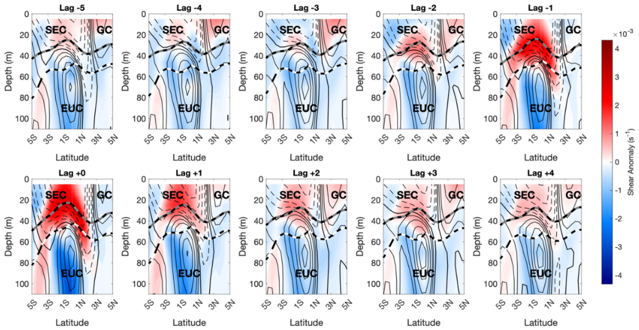
Figure 8.
Same as Figure 7, but for shallow EUC events.
Figure 8.
Same as Figure 7, but for shallow EUC events.
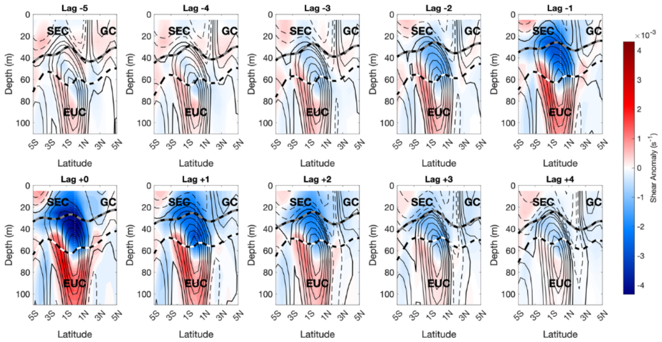
Figure 9.
Spatial composites from Lag -2 to Lag +2 months (top and bottom-left panel) depict SSH anomalies (cm, shaded) overlaid with surface wind anomalies (vectors; bold vectors indicate statistical significance at the 95% confidence level). Bottom-right panel shows the longitude-lag Hovmöller diagram of equatorial SSH anomalies averaged over 4°S–2°N. The black arrow denotes the eastward phase propagation of an upwelling equatorial Kelvin-wave-like signals with an estimated phase speed of
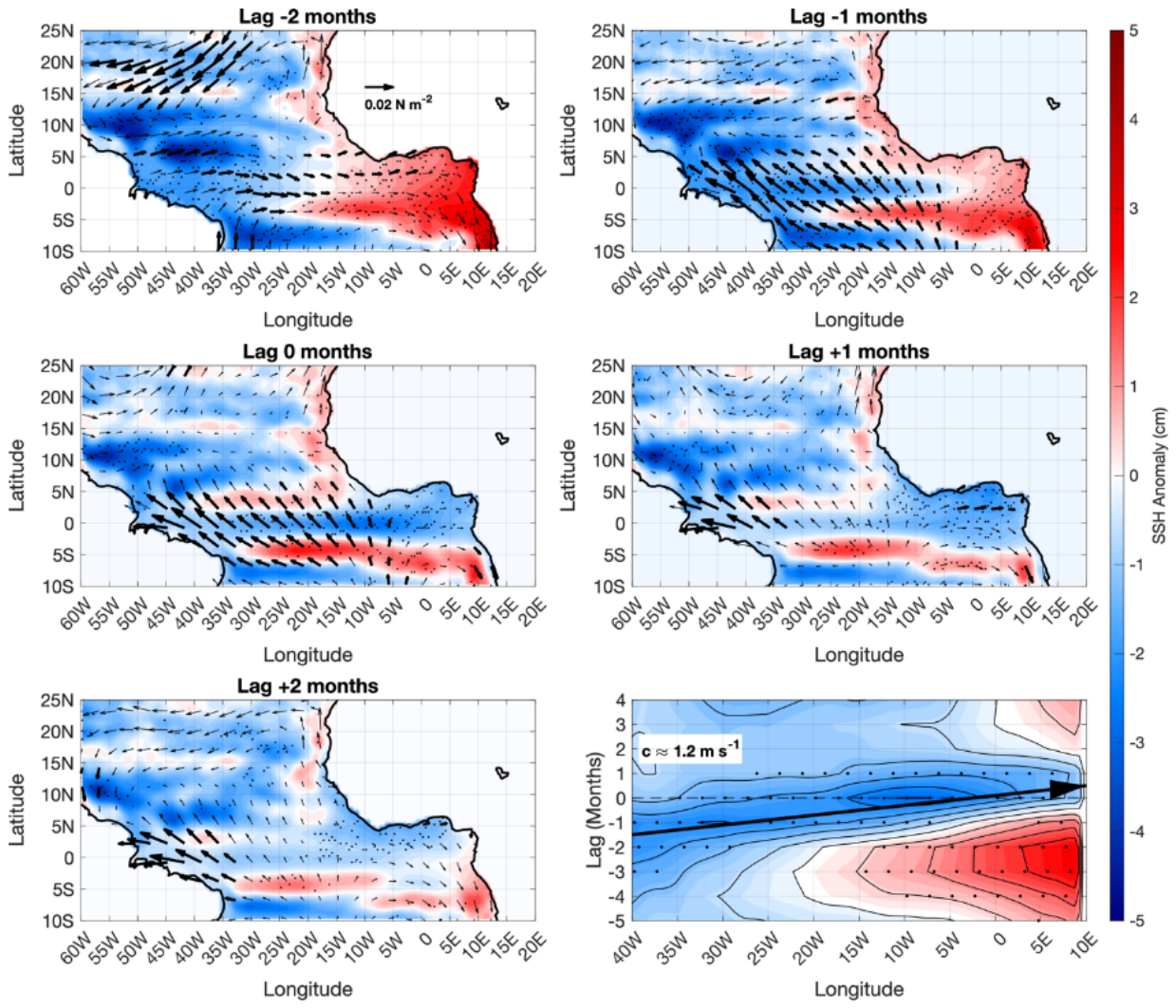
Figure 10.
Same as Figure 9, but for Shallow EUC events. Here, the eastward propagation corresponds to a downwelling equatorial Kelvin-wave-like signals (positive SSH anomalies, shaded red) traveling across the basin at
Figure 10.
Same as Figure 9, but for Shallow EUC events. Here, the eastward propagation corresponds to a downwelling equatorial Kelvin-wave-like signals (positive SSH anomalies, shaded red) traveling across the basin at
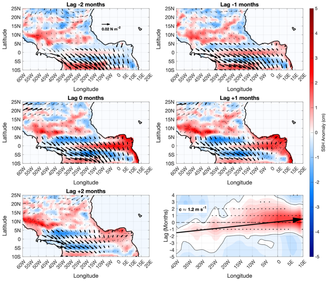
Figure 11.
Composite spatial maps (Lags −5 to +3 months) and longitude-time (Hovmöller) diagram of relative Sea Level Pressure anomalies (SLP, shaded in hPa) and surface wind vector anomalies (u,v, arrows in m s−1) for the Deep EUC regime. Maps depict the Tropical Atlantic domain (60°W–20°E, 10°S–25°N). The Hovmöller panel (bottom right) illustrates the equatorial evolution (40°W–10°E, averaged between 4°S–2°N) relative to wave arrival at Lag 0 (dashed line). Positive/negative lags denote months after/before the peak event. The dotted vertical line highlights the eastern boundary (0∘E).
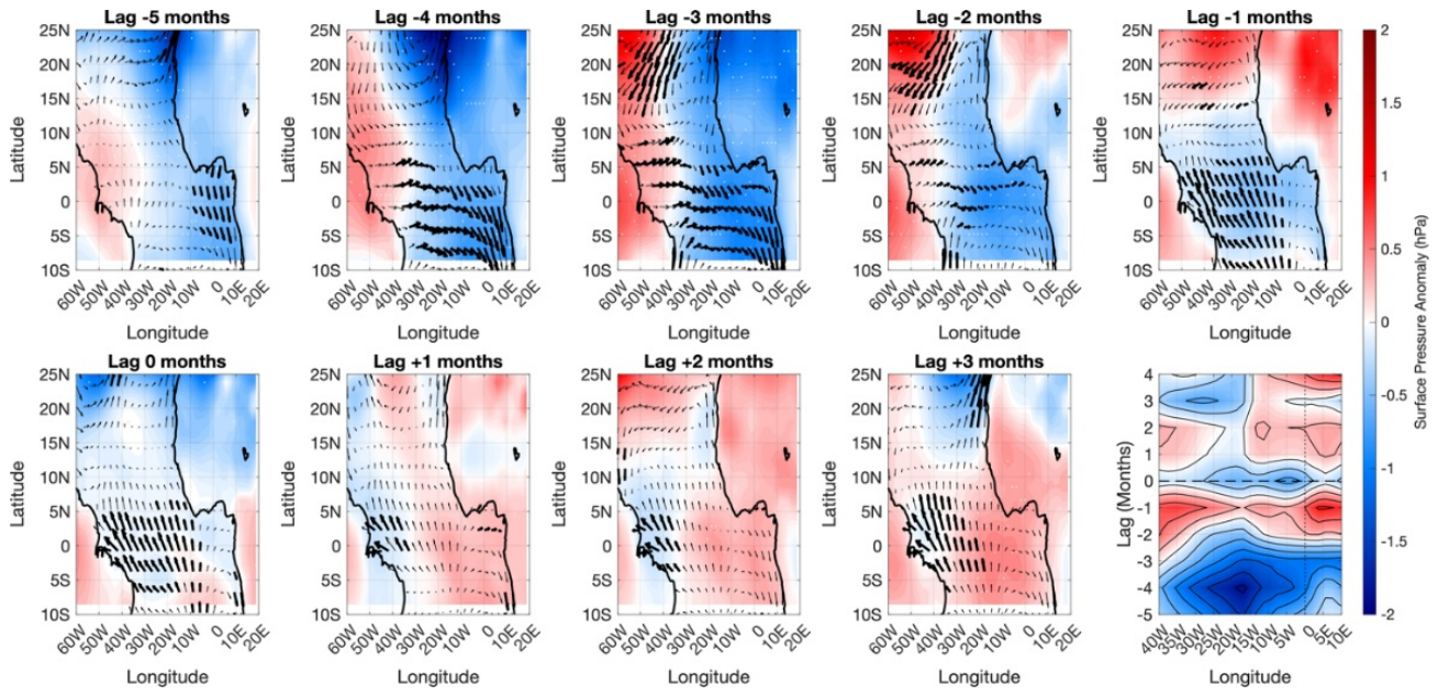
Figure 12.
Same as Figure 11, but for the Shallow EUC regime.
Figure 12.
Same as Figure 11, but for the Shallow EUC regime.
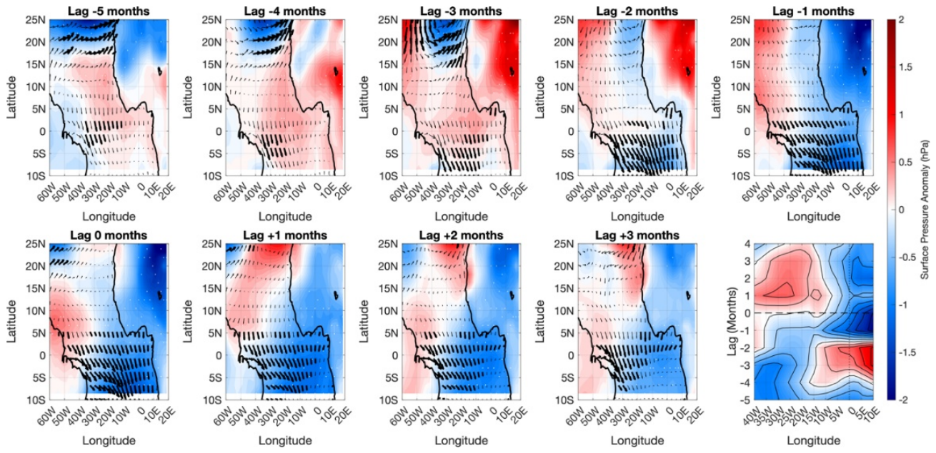
Figure 13.
Composite differences (Deep − Shallow) between anomalously deep and shallow EUC core-position states at Lag 0. (a) Zonal wind-stress difference (Δτx, N m⁻²). (b) Time–longitude (Hovmöller) diagram of sea surface height difference (ΔSSH, cm), averaged between 4°S and 2°N, highlighting the eastward propagation of an upwelling Kelvin-wave-like anomaly (c ≈ 1.2 m s⁻¹; black arrow). (c) Thermocline depth difference (ΔTHD, m). (d) Mixed-layer depth difference (ΔMLD, m). (e) Equatorial longitude–depth section (4°S–2°N average) of ocean temperature difference (ΔT, °C; shading), overlaid with zonal and vertical current anomalies (vectors). The dashed black–white and black–grey lines depict the THD Deep and THD Shallow states, respectively. (f) Sea surface temperature difference (ΔSST, °C; shading) and surface wind-stress vector anomalies (N m⁻²; reference vector: 0.02 N m⁻²). Stippling in (a)–(f) indicates statistical significance at the 95% confidence level.
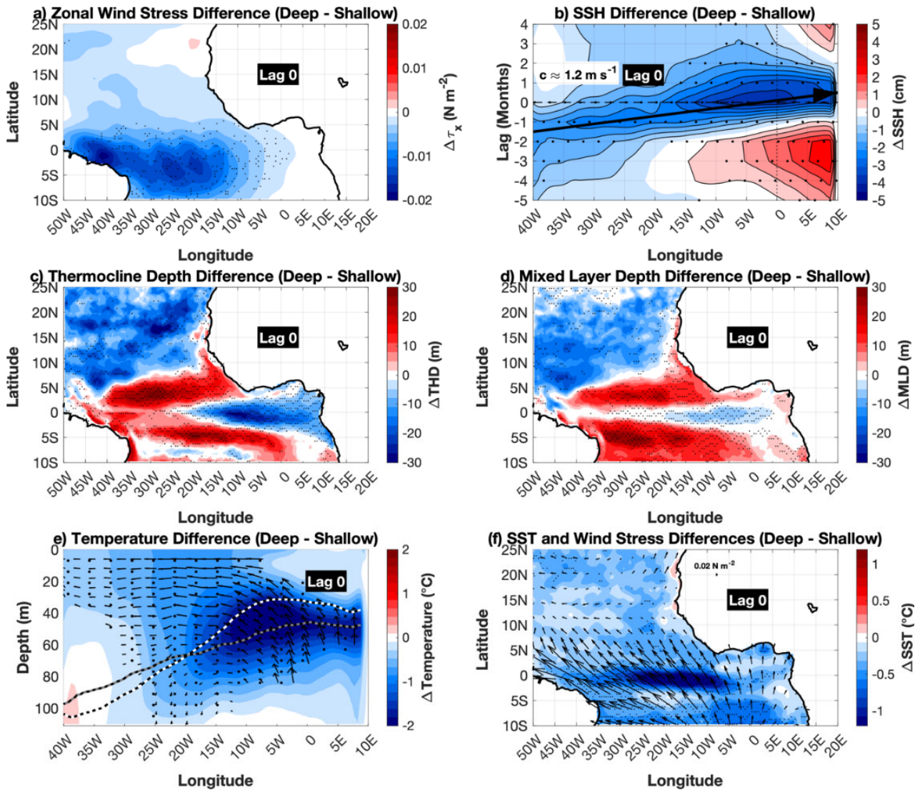

Table 1.
Summary statistics of the independent Deep and Shallow EUC events. The table reports the selection thresholds, number of candidate months, number of independent events, mean event duration, mean EUC vertical position and position anomaly, mean maximum EUC velocity, thermocline depth (THD), and mixed-layer depth (MLD). Values are given as mean ± standard deviation. For the physical diagnostics, values are calculated at the peak month of each independent event.
| Metric | Deep | Shallow |
| Selection threshold | +1σ | −1σ |
| Candidate months | 158 | 136 |
| Independent events | 95 | 84 |
| Mean duration (months) | 1.98 ± 0.79 | 1.89 ± 1.37 |
| Mean EUC position (m) | 87.67 ± 4.07 | 58.10 ± 3.44 |
| Mean EUC-position anomaly (m) | 15.38 ± 4.07 | −14.19 ± 3.44 |
| Mean maximum EUC velocity (m s−1) | 1.15 ± 0.14 | 1.13 ± 0.16 |
| Mean Thermocline Depth (m) | 69.07 ± 7.14 | 71.22 ± 5.84 |
| Mean Mixed Layer Depth (m) | 25.38 ± 1.75 | 24.86 ± 2.54 |
Disclaimer/Publisher’s Note: The statements, opinions and data contained in all publications are solely those of the individual author(s) and contributor(s) and not of MDPI and/or the editor(s). MDPI and/or the editor(s) disclaim responsibility for any injury to people or property resulting from any ideas, methods, instructions or products referred to in the content. |
© 2026 by the authors. Licensee MDPI, Basel, Switzerland. This article is an open access article distributed under the terms and conditions of the Creative Commons Attribution (CC BY) license (http://creativecommons.org/licenses/by/4.0/).
Copyright: This open access article is published under a Creative Commons CC BY 4.0 license, which permit the free download, distribution, and reuse, provided that the author and preprint are cited in any reuse.