

Submitted:
02 October 2026
Posted:
06 October 2026
You are already at the latest version
Abstract
This study extends fractal boundary analysis from national borders to continental and subcontinental landmasses through a 29-unit hierarchical framework comprising six continents and 23 subcontinents, defined under a modified UN M49 structure with study-specific connectivity rules. Each geographical unit was constructed and measured directly from its external perimeter, so parent-continent estimates represent distinct boundary geometries rather than averages or weighted combinations of constituent subcontinental dimensions. Adaptive box-counting (BC) and divider (DIV) estimators were applied under a common finite-scale procedure, followed by descriptive scale-stratified analysis of boundary complexity, parent–subcontinent contrasts, cross-method correspondence, method sensitivity, and equal-weight consensus fractal dimensions (FDs). Continental mean FDs exceeded subcontinental means under both methods (BC: 1.160842 vs. 1.136353; DIV: 1.172651 vs. 1.141075). Cross-method agreement was strong at both scales (continents: Pearson r = 0.9876, Lin CCC = 0.9624; subcontinents: Pearson r = 0.9822, Lin CCC = 0.9743). Greenland and Northern Europe occupied the upper end of the hierarchy, whereas Southern Africa formed the lower extreme. Despite this overall agreement, substantial within-family heterogeneity and localized method-sensitive differences remained. The resulting Continental Atlas provides a reproducible hierarchical framework for characterizing macro- scale boundary complexity while preserving geographical scale, direct perimeter construction, and estimator-specific information.
Keywords:
continent
; border complexity
; fractal dimension
; method agreement
; spatial statistics
1. Introduction
1.1. From National Borders to Continental Landmass Borders
Geographical boundaries are scale-dependent objects whose measured complexity varies with the spatial resolution at which their irregularity is examined. This principle, originating in Richardson’s boundary-length problem and subsequently formalized within fractal geometry by Mandelbrot, applies across a broad range of natural and political geographical boundaries [1,2,3].
Fractal analysis has continued to expand from classical coastline and boundary problems toward larger natural geographical objects, including recent work examining scaling properties across Earth’s islands [4]. Within the present research sequence, the Iran study established the paired adaptive box-counting and divider framework in a national and regional setting [5], while the subsequent Canada study extended the analysis to a broader hierarchy of national, continental, and comparative landmass boundaries [6]. These developments were subsequently consolidated in the worldwide National Border Atlas, which provided harmonized principal-landmass estimates under a common dual-method framework [7].
The present study advances this progression from national borders to continental and subcontinental landmass boundaries. At this larger geographical scale, dissolving internal political boundaries produces new external perimeters, so macro-scale boundary complexity cannot be inferred directly from the dimensions of the countries that compose them. The analytical focus therefore shifts from individual political units to a hierarchy of separately defined geographical landmasses whose scaling behavior can be examined directly.
1.2. Hierarchical Continental and Subcontinental Geography
The Continental Atlas is organized around six continental families and 23 associated subcontinental units. These two levels represent distinct geographical objects rather than successive numerical aggregations: each parent continent and each subcontinent possesses its own external boundary and is therefore measured independently. This hierarchical organization permits boundary complexity to be examined both between geographical scales and within continental families.
The geographical framework draws principally on the United Nations M49 regional structure but is modified where necessary to maintain connected and reproducible landmass configurations [8]. Major study conventions include Eurasia as a single parent landmass, Greenland as a distinct subcontinental member of the North American family, and an Oceania framework centred on its principal connected landmass. These classifications are operational research definitions rather than proposed replacements for official geographical regionalizations; their memberships and connectivity rules are specified in Section 2.2.
1.3. Study Objective and Contributions
The study addresses four related questions: (i) what fractal dimensions characterize the directly measured external boundaries of continents and subcontinents; (ii) how parent-continent dimensions compare with the distributions of their constituent subcontinental dimensions; (iii) how consistently box-counting and divider estimators behave at these two geographical scales; and (iv) whether an equal-weight consensus fractal dimension provides a useful transparent summary while retaining the original method-specific measurements.
The principal contribution is consequently not a re-analysis or numerical aggregation of the National Border Atlas. Instead, the study examines how boundary complexity behaves when the geographical object itself changes from national to larger hierarchical landmasses. This introduces direct parent–subcontinent contrasts, geographical non-additivity, and scale-stratified method concordance as new components of the Atlas framework while preserving methodological continuity with its national-level predecessor [7].
1.4. Study Outline
Section 2 defines the continental–subcontinental hierarchy, geographical construction rules, adaptive fractal-dimension estimators, scaling-window procedure, and descriptive statistical framework. Section 3 presents the direct boundary estimates and examines distributional patterns, cross-method agreement, parent–subcontinent contrasts, method sensitivity, and consensus dimensions. Section 4 interprets these findings in terms of hierarchical boundary complexity, non-additivity, geographical classification, reproducibility, and methodological limitations, followed by the principal conclusions.
2. Methods
2.1. Study Design, Units, and Geospatial Sources
The study was organized as a hierarchical set of 29 geographical records comprising six directly measured continental boundaries and 23 associated subcontinental boundaries. Each record represents a separately constructed exterior landmass boundary at its designated geographical scale. Parent continents and their constituent subcontinents were therefore retained as distinct analytical units: a continental estimate was calculated from the assembled parent boundary itself and was not derived by averaging, weighting, or otherwise combining the corresponding subcontinental estimates.
The hierarchy was structured by continental family, with each subcontinent linked to its parent continent according to the geographical classification and connectivity rules described in Section 2.2. Because parent and descendant boundaries are geometrically related, the 29 records should not be interpreted as a random sample of mutually independent geographical observations. Antarctica forms a parent continent without subcontinental descendants, while other families contain between three and eight defined subcontinental units; the complete compositions are reported in Table 1.
Administrative source geometries were obtained from GADM Version 4.1 [9]. National and territorial polygons required for each study unit were assembled, validated, dissolved, and processed in R Statistical Software [23], principally using the sf and terra spatial packages [11,12]. GADM geometries supplied the boundaries used for fractal-dimension estimation; Natural Earth data were used only as cartographic background for the geographical maps and did not enter the numerical calculations [10].
2.2. Geographical Classification and Connectivity Rules
The geographical hierarchy was developed from the United Nations M49 regional framework, but it was modified where necessary to create analytically coherent connected-landmass units for fractal-boundary measurement [8]. The resulting regions should therefore be regarded as operational research classifications, not as alternative official United Nations continental or subcontinental definitions. Full country and area memberships are provided in Table 1; only the classification and connectivity decisions governing boundary construction are described here.
North America. North America was organized into Northern America, Greenland, and Central America. Northern America and Central America were defined as connected mainland sectors whose union forms the principal North American parent landmass, with Alaska retained because it is physically connected to Canada. Greenland was associated with the North American family but retained as an independent subcontinental unit because it is geographically disconnected from the continental mainland; it was therefore not fused into the parent exterior perimeter. Caribbean island states and other detached island components were outside this connected-mainland construction.
South America. The South American mainland was partitioned into four connected study sectors: Andean States, Southern Cone, Brazilian Sector, and Northeastern States. The Andean designation follows the established Andean regional framework [13,14], while the Southern Cone terminology is supported by its established regional usage [15,16]. The Brazilian and Northeastern sectors are study-specific geographical groupings introduced to complete a non-overlapping connected partition of the South American mainland rather than official M49 subdivisions.
Africa. For Africa, the five M49 regional divisions—Northern, Eastern, Middle, Southern, and Western Africa—provided the primary organizational structure [8]. Their use was adapted to the principal-connected-landmass objective by retaining continental portions where a political unit also contained detached islands or geographically separate components. The resulting five subcontinental boundaries therefore preserve the broad M49 regional organization while ensuring that the geometries entering the analysis form mainland-based spatial units compatible with the boundary-assembly procedure.
Eurasia. Europe and Asia were combined into a single parent continent, Eurasia, because their principal landmasses form one continuous terrestrial system. Within that parent, the M49 structure was modified more substantially to obtain connected analytical subregions: Northern Europe was restricted to Finland, Norway, and Sweden; the remaining connected European mainland was grouped as Mainland Europe; and the principal Russian landmass was represented separately as the Russian Sector. Kaliningrad was assigned to Mainland Europe rather than the Russian Sector because it is detached from the principal Russian landmass but geographically embedded within the European mainland configuration.
The Asian portion of Eurasia was divided into Central, Eastern, Southeast, Southern, and Southwest Asia. Several assignments were made for analytical continuity rather than strict adherence to the standard M49 regional boundaries: Türkiye was included in Southwest Asia in its entirety, together with Armenia, Azerbaijan, and Georgia, while the complete principal Russian landmass—including its European portion—remained within the Russian Sector. These choices avoid introducing an arbitrary physical Europe–Asia cutting line through otherwise continuous national geometries and make the resulting units reproducible from explicit membership and connectivity rules.
Oceania. Oceania required a different treatment because its major landmasses are mutually disconnected. Australia, New Guinea, and New Zealand were therefore retained as separate subcontinental records, with the principal connected component of each geographical object used for analysis. Under the parent-landmass rule, Australia is also the largest connected landmass representing the Oceania parent; consequently, the Oceania and Australia records share the same exterior geometry and therefore the same fractal-dimension estimates. New Guinea and New Zealand remain associated subcontinents but are not artificially joined to Australia to construct a discontinuous parent perimeter.
Antarctica. Antarctica was treated as a single continental geographical unit. No subcontinental partition was introduced because the study objective did not require an internal regionalization of the Antarctic landmass, and doing so would have added a classification scheme not shared with the other principal study framework. Antarctica therefore contributes one directly measured parent boundary and no subcontinental descendant.
Taken together, these rules separate two distinct concepts: geographical affiliation, which determines the continental family to which a unit belongs, and geometrical connectivity, which determines the boundary actually measured. This distinction permits disconnected regions such as Greenland or New Guinea to remain meaningful members of their broader continental families without forcing artificial connections between spatially separate landmasses. The complete membership specification in Table 1 provides the reproducible link between these operational definitions and the boundary-assembly procedure described in Section 2.3. Figure 1, Figure 2 and Figure 3 show the resulting geographical configurations.
2.3. Boundary Assembly and Principal-Landmass Extraction
For each continental or subcontinental record, the contributing GADM 4.1 geometries were processed as one assembled geographical object according to the classification rules of Section 2.2 [9]. Spatial operations were performed principally with sf and terra [11,12]. The boundary-construction procedure consisted of the following ordered steps:
- (i)
- Geographical union: combine all member-country or area polygons assigned to the study unit into a single composite geometry.
- (ii)
- Internal-border dissolution: dissolve shared borders among adjoining members so that only boundaries contributing to the exterior geometry remain.
- (iii)
- Geometry validation: repair invalid polygonal features and verify topology before connected-component analysis.
- (iv)
- Connected-component separation: divide the dissolved geometry into its remaining spatially disconnected polygon components.
- (v)
- Principal-landmass selection: rank the connected components by area and retain the largest connected component as the analytical landmass.
- (vi)
- Interior-ring removal: remove holes and inland-water rings because the study object is the external landmass perimeter rather than internal water boundaries.
- (vii)
- Exterior-boundary extraction: extract the complete outer perimeter of the retained principal landmass without smoothing or geometric simplification.
- (viii)
- Metric projection: transform the retained boundary to a locally centred azimuthal equidistant coordinate reference system in metres for subsequent scale construction and fractal-dimension estimation.
A key difference from the preceding country-level Atlas is the ordering of the first five operations [7]. Here, geographical union and dissolution are performed before principal-component selection, allowing components that are disconnected within an individual national geometry to become connected through another member of the same continental or subcontinental unit. For example, Alaska becomes part of the connected Northern American landmass through its terrestrial connection with Canada after the Canadian and United States geometries are assembled.
Additional topology checks were applied to avoid artificial segments arising from longitude discontinuities. Where a study geometry approached or crossed the antimeridian, longitude handling was performed before planar transformation so that the date-line discontinuity did not generate spurious long edges. The retained boundary itself was otherwise left geometrically unchanged.
The local projection was centred on the retained assembled landmass rather than on the individual source countries. This preserves the object-centred metric framework of the national Atlas while extending it to substantially larger geographical domains. Because planar distortion may become more consequential for very large units such as Eurasia, North America, and Antarctica, projection dependence is treated as an explicit methodological sensitivity of the continental analysis.
2.4. Adaptive Box-Counting and Divider Fractal Dimension Estimations
The adaptive dual-method estimator follows the computational framework of the preceding National Border Atlas and was applied without continent-specific retuning to each newly constructed continental and subcontinental boundary [7]. The principal change is therefore the analytical object rather than the estimator: candidate scales and both fractal-dimension calculations were generated anew from the projected assembled boundary defined in Section 2.3. This preserves methodological continuity and consistency across the Atlas series while allowing the scale range to adapt automatically to the substantially larger geographical units.
As in previous Atlas [7], for a projected boundary with shorter bounding-box side s, the standard-profile coarsest candidate scale was
Let denote the 25th percentile of native boundary-segment lengths and the projected bounding-box area. With the inherited nominal floor km and maximum grid size cells, the finest admissible candidate was
The standard candidate scales were then logarithmically spaced between and ,
These resolution and finite-scale constraints follow the same rationale used in the National Border Atlas and avoid extrapolation below the effective information content of the source geometry [17,18].
For box counting, square grids of side length r were superimposed on the projected exterior boundary. Multiple translated grid origins were evaluated at each candidate scale, and the minimum occupied-cell count was retained,
thereby reducing dependence on an arbitrary grid origin. Scales with fewer than eight occupied cells were excluded. Following the standard box-counting relation [2], the selected log–log regression was written as
Supporting calculations used the fractaldim implementation where applicable [19].
The divider estimator independently evaluated the same exterior boundary through Richardson scaling [1]. After boundary densification, divider traversals were performed over admissible ruler lengths r, with measured boundary length defined as . Under , the fitted relationship
gave
Thus, box counting and divider measurement were applied as geometrically distinct estimators to the same assembled boundary, permitting cross-method agreement and sensitivity to be evaluated at both continental and subcontinental scales.
No geographical unit was assigned a manually chosen scaling interval or estimator-specific tuning parameter. The same inherited candidate-scale construction and dual-method rules were applied across the hierarchy, so differences among the resulting estimates arise from the assembled boundary geometries and the subsequent adaptive window selection rather than from unit-specific calibration.
2.5. Scaling-Window Selection, Diagnostics, and Archiving
Scaling intervals were selected independently for the box-counting and divider estimators using the objective rule inherited from the National Border Atlas [7]. Rather than prescribing one common interval across geographical units, the procedure evaluates the finite-scale behavior of each newly assembled continental or subcontinental boundary and selects a supported interval from its admissible candidate scales. The essential selection rules are summarized in Table 2.
The selected fit was retained with its fractal-dimension estimate, statistics, scale limits, and method-specific diagnostics. Box-counting and divider windows were selected independently, so differences between their retained intervals were preserved as part of the observed method sensitivity.
For reproducibility, each geographical-unit record archives its source membership, assembled and projected boundary, candidate scales, method measurements, examined windows, selected regressions, diagnostics, and final outputs. This extends the National Border Atlas archive by adding the continental–subcontinental construction layer [7].
The overall 10-step computational procedure—including translated box-count evaluation, divider traversal, regression fitting, window diagnostics, and output generation—follows exactly the workflow used in the National Border Atlas; interested readers may refer to that study for the complete procedural details [7].
2.6. Statistical Analysis
Statistical summaries were performed separately for the six continental and 23 subcontinental records, with no pooled 29-unit analysis. For each geographical scale, box-counting and divider estimates were summarized using the mean, standard deviation (SD), median, quartiles, range, and percentage departure from the linear benchmark,
Cross-method correspondence was evaluated separately at each scale using Pearson correlation, Spearman rank correlation [20], and Lin’s concordance correlation coefficient (CCC) [21]. For each geographical unit, the signed and absolute method differences were defined as and with interpretation distinguishing association from numerical agreement [22,24].
Parent–subcontinent structure was summarized by comparing each directly estimated parent-continent dimension with the median and range of its associated subcontinental estimates. An equal-weight descriptive consensus dimension was also calculated for every unit as
Finally, given that the geographical units are predefined, hierarchically nested, partly overlapping, and not independent random observations, the assumptions underlying conventional inferential procedures are not adequately satisfied. Hence, the statistical analysis was restricted to descriptive and agreement-based summaries.
3. Results
3.1. Unit-Level Fractal Dimension Estimations
Table 3 presents the adaptive box-counting and divider fractal-dimension estimates for the six continental and 23 subcontinental geographical units. Each parent-continent estimate is obtained directly from the complete assembled boundary of that continent and is therefore not an average, weighted combination, or other summary of its constituent subcontinental estimates. Accordingly, differences between a parent continent and its subcontinents reflect the geometry of separately defined geographical boundaries rather than an averaging relationship. Across the study units, the selected regressions generally exhibited high coefficients of determination, while the retained scale windows varied by geographical unit and estimation method under the adaptive procedure.
North America. The North American parent boundary yielded box-counting and divider dimensions of 1.223342 and 1.247389, with corresponding values of 0.999967 and 0.998317. The box-counting fit extended over 5.8193–200.0000 km, whereas the divider window was 5.8193–87.0123 km. Subcontinental estimates showed a pronounced internal contrast: Greenland attained the highest values in the family (; ), while Central America was substantially lower (1.129626 and 1.138308, respectively); Northern America occupied an intermediate position with estimates of 1.242453 and 1.262083.
South America. For South America, the parent-continent dimensions were 1.135864 by box counting and 1.154465 by the divider method, with strong fits of and , respectively. The box-counting scaling interval extended from 5.0582 to 200.0000 km, while the divider fit retained 5.0582–84.1894 km. Among the four subcontinents, the Southern Cone was distinctly higher under both methods (1.164441 and 1.180001), whereas the Andean States, Brazilian Sector, and Northeastern States remained clustered closer to approximately 1.08–1.10. Thus, the directly estimated South American parent boundary exceeded most of its subcontinental estimates but remained below the Southern Cone.
Africa. Africa produced parent-continent estimates of and , with values of 0.999937 and 0.995627. Its selected box-counting window covered 6.3381–200.0000 km, compared with 6.3381–48.2797 km for the divider fit. The five African subcontinents occupied a comparatively narrow dimensional range, although Western Africa had the largest paired estimates (1.081876 and 1.093631), closely approaching the parent-continent values, while Southern Africa had the smallest (1.046781 and 1.030536). The remaining Northern, Eastern, and Middle African units lay between these two patterns, with consistently high regression fits despite differing retained scale intervals.
Eurasia. The Eurasian parent boundary had box-counting and divider dimensions of 1.185642 and 1.194468, respectively, and both methods retained the same broad 8.6294–200.0000 km scaling interval, with and . The principal subcontinental contrast was Northern Europe, whose estimates of 1.290143 and 1.348592 were markedly higher than both the Eurasian parent and the other Eurasian subcontinents. At the lower end, Southwest Asia produced nearly identical estimates under the two methods (1.099926 and 1.099913), while the remaining European and Asian units occupied the intervening range. Despite this comparatively broad spread in fractal dimension, fit statistics remained uniformly high across the Eurasian family.
Oceania. The Oceania parent boundary was estimated at 1.149449 by box counting and 1.152129 by the divider method, with corresponding values of 0.999880 and 0.997222. The retained scale windows were 2.9159–200.0000 km and 2.9159–121.6184 km, respectively. The Oceania parent and Australia subcontinental entries were numerically identical under both methods, while New Guinea was slightly lower (1.134132 and 1.130259) and New Zealand was higher (1.180630 and 1.179499). The very small cross-method differences for all three subcontinental units indicate close numerical correspondence between the two estimators within this continental family.
Antarctica. Antarctica, for which no subcontinental units were defined, yielded closely aligned box-counting and divider estimates of 1.192644 and 1.196504. Both regressions were strong ( and ), with broad selected scale windows of 3.8820–200.0000 km for box counting and 6.1725–200.0000 km for the divider method. The small difference between the two estimates and the broad retained scaling intervals provide a consistent dual-method characterization of the Antarctic parent boundary.
0pt
0pt 0pt
3.2. Statistical Analysis
3.2.1. Continental and Subcontinental Fractal Dimension Distributions
Table 4 summarizes the scale-stratified distributions of the continental and subcontinental fractal-dimension estimates. At the continental scale, the mean box-counting and divider dimensions were 1.160842 and 1.172651, respectively, compared with 1.136353 and 1.141075 at the subcontinental scale, indicating that the directly measured continental boundaries were, on average, more fractally complex than the subcontinental boundaries under both methods. Divider estimates were also slightly higher than the corresponding box-counting estimates at each geographical scale. In contrast, the subcontinental distributions were more heterogeneous, with larger standard deviations under both box counting (0.071797 vs. 0.051247) and the divider method (0.080180 vs. 0.053023), together with wider observed ranges, particularly for the divider estimates. The corresponding departures from the linear benchmark were 16.08% and 17.27% for continents and 13.64% and 14.11% for subcontinents, reinforcing the same scale-level patterns.
3.2.2. Cross-Method Agreement and Concordance
Table 5 summarizes cross-method association, concordance, and paired differences separately at the continental and subcontinental scales. Box-counting and divider estimates showed very high linear association at both scales, with Pearson coefficients of for the six continents and for the 23 subcontinents, while Spearman correlations of and , respectively, indicated similarly strong preservation of rank ordering. Numerical concordance was also high, with Lin’s CCC equal to 0.9624 at the continental scale and 0.9743 at the subcontinental scale. Mean box-counting minus divider differences were negative for both groups ( and ), indicating that divider estimates were, on average, slightly larger, whereas the corresponding mean absolute differences were small and similar in magnitude (0.011810 and 0.011191). Taken together, these results indicate close cross-method correspondence at both geographical scales, although the continental coefficients should be interpreted descriptively and cautiously because they are based on only six continental units.
Figure 4 provides a visual counterpart to the cross-method agreement results. The continental and subcontinental estimates form a clear ascending pattern and are generally concentrated near the line, indicating that units with higher box-counting dimensions also tend to have higher divider dimensions across both geographical scales. Most parent-continent estimates lie close to equality, while Northern Europe shows the most prominent visible departure above the line, reflecting a comparatively larger divider estimate; Greenland, by contrast, lies slightly below equality. Overall, the configuration supports strong cross-method consistency across the continental hierarchy while identifying a small number of geographically specific method-sensitive differences. In broad descriptive terms, the lower-dimensional portion of the figure is occupied predominantly by the African family, including Southern, Northern, Eastern, and Middle Africa, followed by Western Africa and the African parent unit. The lower-to-middle range then contains several South American and Asian units, including the Andean States, Brazilian Sector, Northeastern States, Southwest Asia, Central Asia, and Central America, whereas the middle-to-upper range includes Eastern and Southeast Asia, Oceania and Australia, Mainland Europe, the Russian Sector, New Zealand, the Southern Cone, and the South American parent. At the upper end, Eurasia and Antarctica are followed by North America and Northern America, with Greenland and Northern Europe forming the highest-dimensional macro-scale group in the figure.
3.2.3. Continent-Subcontinent Boundary Complexity
Table 6 compares each directly measured parent-continent boundary with the median and range of its associated subcontinental estimates. The parent values were generally not equal to the corresponding subcontinental medians, reinforcing that continental fractal dimensions were obtained from the complete parent boundary rather than by arithmetic aggregation of subcontinental estimates. This contrast was particularly evident for Eurasia, whose parent estimates (, ) exceeded the subcontinental medians (1.141383 and 1.146379), while its subcontinents also exhibited the broadest within-family ranges, extending from 1.099926 to 1.290143 for box counting and from 1.099913 to 1.348592 for the divider method. Africa showed a much narrower subcontinental spread, whereas South America likewise had parent estimates above its corresponding subcontinental medians. North America showed comparatively close parent-to-median alignment, and Oceania was especially closely aligned because the parent Oceania estimate and the Australia subcontinent share identical paired values in the dataset. Antarctica stands separately as a parent continent with no defined subcontinental descendants, so no within-family median or range is applicable.
3.2.4. Method-Difference Sensitivity
Table 7 identifies the four geographical units with the largest observed absolute differences between the box-counting and divider estimates. Northern Europe showed the greatest discrepancy (; ), followed by Central Asia (), North America (), and Northern America (). In all four cases, was negative, indicating that the divider estimate exceeded the corresponding box-counting estimate. These values represent the largest observed method-specific discrepancies in the continental–subcontinental dataset and should be interpreted descriptively rather than as tests of statistical significance or method interchangeability. Their interpretation should also be considered together with the selected scaling-window diagnostics, since the two estimators may retain different finite-scale intervals for the same geographical boundary.
3.2.5. Consensus Fractal Dimensions
Table 8 summarizes the box-counting, divider, and equal-weight consensus fractal dimensions for the six continents and 23 subcontinents. For each geographical unit, the consensus value is defined as the transparent descriptive midpoint , and therefore necessarily lies between the two method-specific estimates; it should not be interpreted as a variance-optimal or uncertainty-weighted estimator. Because the cross-method differences are generally small, the consensus ordering closely preserves the broad hierarchy already observed under the separate estimators. Greenland has the highest consensus value in the complete continental–subcontinental dataset (), followed closely by Northern Europe (1.319368), whereas Southern Africa occupies the lower extreme (1.038658). At the parent-continent level, North America has the highest consensus dimension (1.235365), followed by Antarctica (1.194574) and Eurasia (1.190055), while Africa has the lowest parent-continent value (1.084530). Overall, the consensus measure provides a compact single-number summary of the paired estimates while retaining the principal family-level contrasts apparent under both original methods.
Figure 5 provides a visual comparison of the box-counting, divider, and consensus dimensions across the six continental families, with each parent continent followed by its associated subcontinental units. The figure reinforces the broad hierarchical structure of the results: the African family occupies predominantly the lower-dimensional range, South American and several Asian subcontinents are concentrated in the lower-to-middle range, Oceania and the European–Asian units extend through the middle-to-upper range, and the highest values occur within the North American and northern Eurasian families. Greenland and Northern Europe are visually prominent at the upper end, whereas Southern Africa remains distinctly lower than the other units. For most geographical units, the three bars are closely aligned, showing that the consensus value tracks the two original estimators without materially changing their broad ordering; the largest visible separations occur for method-sensitive units such as Northern Europe and Central Asia. Thus, Figure 5 summarizes both the macro-scale progression of boundary complexity across continental families and the localized cross-method differences retained within that hierarchy.
4. Discussion
4.1. Main Continental and Subcontinental Complexity Patterns
The continental-scale analysis reveals a structured hierarchy of border complexity that is not apparent from country-level summaries alone. Across the six continents and 23 subcontinents, two main results identify clear differences in the magnitude and geographical distribution of finite-scale fractal complexity.
First, the estimated dimensions span a moderate but clearly non-linear range, extending from Southern Africa at the lower end to Greenland and Northern Europe at the upper end. The geographical units therefore exhibit substantial macro-scale heterogeneity while remaining far from plane-filling geometry. As in the preceding country level Atlas [7], these values should be interpreted as finite-scale descriptors of the represented boundaries rather than resolution-independent constants [2,17,18].
Second, a distinct family-level structure is evident. The African units are concentrated predominantly within the lower-dimensional range, whereas the North American family and northern Eurasian units occupy much of the upper range; South America, Oceania, and the remaining Eurasian subcontinents largely span the intermediate region. This pattern indicates that continental boundary complexity varies systematically across geographical families while retaining substantial heterogeneity within individual continental systems.
4.2. Parent-Subcontinent Contrasts and Non-Additivity
A central feature of the present Atlas is that a parent continent and its constituent subcontinents represent different geographical objects. Consequently, the continental fractal dimension is not an aggregation of the corresponding subcontinental dimensions, but a direct measurement of the newly assembled external boundary. This distinction provides an important hierarchical interpretation of the contrasts reported in Table 6.
First, dissolving the constituent geographical units removes their shared internal borders and retains only the exterior perimeter of the resulting connected landmass. In set-theoretic terms, the boundary of a union is generally not the union of the individual boundaries(indeed, ). The parent continent therefore possesses a new boundary geometry whose scaling structure may differ substantially from those of its components [2,3].
Second, fractal dimension itself is not additive across component boundaries. Box-counting and divider dimensions are obtained from scale-dependent relationships between boundary measurement and spatial resolution, rather than from quantities that can be summed or arithmetically averaged [17,18]. Accordingly, neither the mean nor a weighted mean of the subcontinental dimensions can, in general, reconstruct the dimension obtained directly from the dissolved parent boundary.
Third, the observed parent–subcontinent contrasts should therefore be interpreted as genuine consequences of geographical reassembly rather than discrepancies between hierarchical levels. Eurasia and South America, for example, have parent estimates above their corresponding subcontinental medians, whereas other families show closer alignment (Table 6). Such relationships demonstrate that changing the geographical unit changes the boundary being measured, making continental complexity an emergent property of the assembled external perimeter rather than a simple summary of its constituent fractal dimensions.
4.3. Cross-Method Agreement and Method Sensitivity
The box-counting and divider estimators show strong overall correspondence across both levels of the continental hierarchy, while retaining a limited number of larger unit-specific differences. Importantly, association, rank preservation, and numerical agreement describe related but distinct properties and should not be treated as interchangeable measures of method agreement [22].
First, Pearson correlations indicate very strong linear association between the two estimators, with for continents and for subcontinents. Thus, units with larger box-counting dimensions generally also have larger divider dimensions. These coefficients describe the strength of linear association, however, and do not by themselves establish numerical equivalence between the two methods [22,24].
Second, Spearman rank correlations were similarly high, with at the continental scale and at the subcontinental scale. The geographical ordering of boundary complexity is therefore strongly preserved when the estimation method changes, particularly among the 23 subcontinents. Rank agreement nevertheless concerns relative ordering rather than equality of the paired numerical estimates [20].
Third, Lin’s concordance correlation coefficients provide a more direct assessment of numerical agreement relative to the identity line [21]. The corresponding values of for continents and for subcontinents indicate substantial concordance beyond simple correlation [24]. Together with the concentration of most observations near the line, these results support substantial numerical consistency between the two estimators.
Finally, the paired-difference measures reveal the localized method sensitivity that remains beneath this strong overall agreement. Mean differences were small at both scales ( and ), as were the mean absolute differences (0.011810 and 0.011191), although Northern Europe, Central Asia, North America, and Northern America showed the largest individual discrepancies. These cases reinforce that strong global association and concordance do not imply complete interchangeability for every geographical boundary [22,25].
4.4. Geographical Classification Choices and Reproducibility
The continental hierarchy used in this Atlas is an operational geographical framework constructed for connected-boundary analysis rather than a proposal for a new official world regionalization. Its purpose is to define reproducible geographical objects whose exterior boundaries can be assembled consistently from GADM or other available open source data geometries while retaining recognizable continental and subcontinental structure [8,9].
First, the United Nations M49 classification provides the principal reference framework, but several study-specific modifications were required to preserve connected principal-landmass units [8]. The resulting taxonomy therefore follows M49 where compatible with the analytical objective while modifying selected memberships, names, and territorial treatments when necessary for geographical connectivity. These departures are recorded explicitly in Table 1 rather than being treated as implicit classification assumptions.
Second, Europe and Asia are represented jointly as the parent continent Eurasia. Within this parent boundary, European and Asian subcontinents remain separately identifiable, including Northern Europe, Mainland Europe, the Russian Sector, and the specified Asian regions. This convention permits the complete connected Eurasian landmass to be measured as one parent geographical object while preserving internal regional structure for subcontinental comparison.
Third, Greenland is retained within the North American continental family but treated as a separate subcontinental unit rather than merged with Northern America. This preserves its geographically distinct principal landmass and prevents its large autonomous exterior perimeter from being absorbed into the Canada–United States boundary assembly. The treatment is therefore analytical and connectivity-based while remaining transparent relative to the broader M49 regional framework [8].
Fourth, Oceania illustrates an important consequence of the principal-connected-landmass rule. Although Australia, New Guinea, and New Zealand are retained as distinct subcontinental units, the directly measured Oceania parent boundary is numerically identical to the Australia boundary because Australia is the principal connected landmass of the assembled Oceania configuration. This equality is therefore a geometrical consequence of the study definition rather than independent replication of the Australian estimate.
Finally, these classifications should be understood as operational study regions rather than replacements for official geographical, political, or statistical classifications. Reproducibility therefore depends not only on the estimation algorithms but also on explicit documentation of unit membership, exclusions, disconnected components, and connectivity rules. By reporting those decisions alongside the GADM source geometries, the Atlas makes the geographical construction itself part of the reproducible analytical framework [9].
4.5. Interdisciplinary Scope and Potential Applications
Beyond geographical description, the continental and subcontinental dimensions provide standardized macro-scale measures of landmass-boundary complexity within an explicitly hierarchical framework. Their principal interdisciplinary value lies in applications where coastline irregularity, geographical scale, or the geometry of spatial aggregation is itself relevant. Two qualifications apply throughout. First, the composition of the measured perimeters differs between hierarchical levels: parent-continent perimeters are predominantly coastline, with only short terrestrial segments where continental families meet, such as the Panama–Colombia boundary, whereas many subcontinental perimeters combine coastline with land borders shared with neighbouring subcontinents, and some, such as Central Asia, contain no open-ocean coastline. Coastal applications therefore pertain chiefly to the parent continents and to coastline-dominated subcontinents such as Greenland, Northern Europe, Australia, New Guinea, and New Zealand. Second, the coastlines are those represented in the GADM 4.1 administrative geometries rather than in a dedicated shoreline product, so coastline-specific applications would benefit from the replication against high-resolution shoreline databases proposed in Section 4.6 [27].
Geomorphology and Tectonic Geology. At the parent-continent scale, fractal dimension provides a compact descriptor of large-scale perimeter irregularity that may be compared with tectonic setting, erosional history, glacial inheritance, or sea-level-driven coastal evolution. In a study of the Italian coastline, D’Alessandro et al. related differences in fractal dimension among coastal sectors to tectonic activity, wave erosion, postglacial eustatic fluctuations, and volcanism [28], suggesting a basis for analogous comparisons among major continental margins. Within the present hierarchy, the highest values occur for Greenland and Northern Europe, whose coastlines are extensively fjorded, whereas the African family occupies the lower range; such correspondences remain descriptive. Because a single parent estimate integrates margins of very different origin, as in Eurasia, process-oriented interpretation would be better supported at subcontinental or coastal-segment level than by the six parent values alone.
Oceanography and Numerical Earth-System Modeling. Coastline complexity directly affects how land–ocean boundaries are represented on numerical grids. Liu et al. showed that grid generation for regional ocean models involves a trade-off between grid orthogonality and alignment to irregular coastlines, and recommended that the multi-scale fractal characteristics of the coastline be considered in grid design [29]. Under the divider relation , the estimated dimension describes how the represented boundary length changes with resolution r within the retained scaling window. Because the selected continental windows extend from a few kilometres to 200 km, a range that overlaps commonly used horizontal resolutions of regional and global ocean models, the Atlas dimensions may provide macro-scale reference measures for resolution sensitivity and coastline representation in ocean and Earth-system models.
Coastal-Zone Classification and Biogeochemistry. Bartley et al. proposed coastline complexity, measured as plan-view tortuosity by an angle-measurement technique applied to global shoreline data, as a parameter for the functional classification of coastal environments and for understanding coastal biogeochemical processes [30]. Although their angle-based measure differs from the box-counting and divider estimators used here, both quantify scale-dependent coastline irregularity. Parent-continent and coastline-dominated subcontinental dimensions could therefore provide broad comparative context for global coastal-zone classification. Such classification, however, operates at much finer coastal-segment scales, and regional or local coastal processes should not be inferred directly from macro-scale values.
Spatial Statistics and Hierarchical Regionalization. The parent–subcontinent structure provides an empirical setting for examining how a spatial descriptor changes when the geographical unit changes. This behaviour is analogous to the scale and zoning effects of the modifiable areal unit problem, which Dark and Bram emphasized as a concern for quantitative physical geography as well as human geography [31]. The analogy is partial, because the descriptor here is a geometric property of each unit’s boundary rather than an attribute aggregated over its interior. The present hierarchy also captures a single change of scale, from subcontinent to continent, under one zoning. Alternative continental or subcontinental partitions could therefore be used to investigate the sensitivity of boundary-complexity measures to hierarchical regionalization.
Fractal Geometry and Geometric Measure Theory. The Atlas also provides a geographical empirical example of how boundary geometry changes under set assembly. Dissolving internal boundaries creates a new parent perimeter, and because (Section 4.2), the monotonicity and finite stability of the upper box-counting dimension imply that, in the limiting sense, the dimension of the parent boundary cannot exceed the largest dimension among the component boundaries from which it is assembled, to the extent that the parent perimeter is contained in the union of the retained subcontinental perimeters [32]. Dimensions therefore combine through a maximum rather than an average, providing a theoretical counterpart to the non-additivity discussed in Section 4.2. The finite-scale estimates are consistent with this bound: in every family with subcontinental descendants, both parent estimates lie at or below the largest estimate among the subcontinents forming the parent perimeter (Table 3), noting that the detached Greenland unit is not part of the North American parent perimeter. This hierarchy may therefore serve as an empirical testbed for examining how theoretical properties of box dimension, boundary operations, and geometrical aggregation are reflected in finite-scale estimation.
4.6. Limitations and Future Extensions
The continental framework introduces several limitations that arise specifically from constructing and measuring very large hierarchical geographical units. These concern the source geometries, connectivity rules, finite scaling intervals, and spatial representation of continental boundaries. They also define several natural directions for extending the present Atlas.
First, all reconstructed boundaries remain conditional on the GADM 4.1 source geometries [9]. At continental scale, small differences in national shoreline resolution, vertex density, or boundary representation may accumulate along very long assembled perimeters. Replication with independently constructed global boundary products would therefore provide an important assessment of source-geometry sensitivity.
Second, the topology and connectivity rules used to construct each geographical unit necessarily influence the object being measured. Dissolving internal borders, excluding disconnected islands, and selecting particular connected components determine which perimeter survives as the analytical boundary. Alternative connectivity conventions could consequently generate different parent geometries even when the same underlying national polygons are used.
Third, the reported dimensions characterize scaling only over the finite intervals retained by the adaptive procedure and should not be interpreted as asymptotic geographical constants [17,18]. The substantial differences in selected scale windows among geographical units and between methods indicate that the effective scaling domain remains object-specific. Future sensitivity analyses could examine how alternative admissibility and window-selection criteria affect the continental estimates.
Fourth, projection effects deserve particular attention for exceptionally large landmasses such as Eurasia and North America. A single continent-centered planar projection necessarily represents a much greater spatial extent than the country-level geometries considered in the preceding Atlas [7]. Future work could therefore compare alternative projection strategies or geographically partitioned calculations to quantify the stability of the estimated scaling relationships over very large domains.
Fifth, Antarctica constitutes a distinctive case because it is represented as a single continent without subcontinental descendants and its measured perimeter depends directly on the adopted source representation of the Antarctic boundary. Its estimates should therefore be interpreted within that specific geographical definition rather than assumed to characterize every possible Antarctic coastline convention. Alternative Antarctic boundary representations would provide a useful dedicated sensitivity analysis.
Finally, future extensions should replicate the continental hierarchy using independent global products, including geoBoundaries for administrative geometries [26] and high-resolution shoreline databases where coastline-specific representation is required [27]. Such comparisons could separate boundary-source effects from estimator effects and extend the Atlas toward alternative connectivity conventions, island-inclusive continental systems, and explicitly shoreline-based continental measurements.
Conclusions
In sum, this Continental Atlas shows that continent- and subcontinent-scale boundaries exhibit measurable fractal complexity and substantial geographical heterogeneity within a common analytical framework. Direct estimation of parent continents and their constituent subcontinents demonstrates that boundary complexity is scale-dependent and non-additive, because each hierarchical level represents a distinct geographical perimeter rather than an arithmetic combination of lower-level estimates. Box-counting and divider methods show strong association, rank preservation, and numerical concordance across the continental hierarchy, while retaining localized method-sensitive differences that preclude complete interchangeability. Taken together, the study extends the preceding national-border Atlas into a reproducible hierarchical landmass framework and establishes a standardized basis for comparing continental and subcontinental boundary complexity under common geographical, computational, and adaptive-scale rules.
Funding
This research received no external funding.
Data Availability Statement
All public datasets and associated R software codes used in this study are available in the supplementary materials.
Acknowledgments
This article is dedicated to the human civilization, and to humanity’s enduring pursuit of knowledge, peace, prosperity, and understanding across more than five millennia. The author would like to thank his wife for her invaluable technical support while working on this article.
Conflicts of Interest
The author declares no conflicts of interest.
Abbreviations
The following abbreviations are used in this article: BC, box counting; CCC, concordance correlation coefficient; DIV, divider; FD, fractal dimension; GADM, Global Administrative Areas; M49, United Nations Standard country or area codes for statistical use; PED0, percentage departure from the linear benchmark D0=1; Q1, first quartile; Q3, third quartile; SD, standard deviation; USA, United States of America.
References
- Richardson, L. F. (1961). The problem of contiguity: An appendix to statistics of deadly quarrels. General Systems Yearbook, 6, 139–187.
- Mandelbrot, B. B. (1967). How long is the coast of Britain? Statistical self-similarity and fractional dimension. Science, 156(3775), 636–638.
- Longley, P. A., & Batty, M. (1989). On the fractal measurement of geographical boundaries. Geographical Analysis, 21(1), 47–67. [CrossRef]
- Oline, M., Hoskins, J., Seekell, D., Silber, M., & Cael, B. B. (2026). Self-affine scaling of Earth’s islands. Geophysical Research Letters, 53, e2025GL121272. [CrossRef]
- Soltanifar, M. (2026). Fractal dimensions of modern Iran’s borders, the Persian Gulf, and the Caspian Sea coastlines [Preprint]. Preprints.org. [CrossRef]
- Soltanifar, M. (2026). Fractal dimensions of Canada’s borders and coastlines [Preprint]. Preprints.org. [CrossRef]
- Soltanifar, M. (2026). A World Statistical Atlas of National Border Fractal Dimensions. [Preprint]. Preprints.org. [CrossRef]
- United Nations Statistics Division. (n.d.). Standard country or area codes for statistical use (M49). United Nations. Retrieved September 27, 2026, from https://unstats.un.org/unsd/methodology/m49/.
- Global Administrative Areas (GADM). (2022). GADM database of global administrative areas (Version 4.1) [Data set]. https://gadm.org/.
- Natural Earth. (n.d.). Natural Earth I with shaded relief and water & Natural Earth 10m physical vectors: Lakes and reservoirs (Version 3.2.0) [Raster data sets]. Retrieved August 31, 2026, from https://www.naturalearthdata.com.
- Pebesma, E. (2018). Simple features for R: Standardized support for spatial vector data. The R Journal, 10(1), 439–446. [CrossRef]
- Hijmans, R. J. (2026). terra: Spatial data analysis (R package Version 1.9-34) [Computer software]. Comprehensive R Archive Network. https://CRAN.R-project.org/package=terra.
- Andean Community. (1969, May 26). Andean Subregional Integration Agreement (Cartagena Agreement). https://www.comunidadandina.org/quienes-somos/.
- Andean Community. (n.d.). Member countries. Retrieved September 27, 2026, from https://www.comunidadandina.org/quienes-somos/paises-miembros/.
- Steves, F. (2001). Regional integration and democratic consolidation in the Southern Cone of Latin America. Democratization, 8(3), 75–100. [CrossRef]
- Majstorović, G. (2022). The Southern Cone novel (Argentina, Chile, Uruguay, and Paraguay). In J. E. De Castro & I. López-Calvo (Eds.), The Oxford handbook of the Latin American novel (pp. 258–275). Oxford University Press. [CrossRef]
- Carr, J. R., & Benzer, W. B. (1991). On the practice of estimating fractal dimension. Mathematical Geology, 23(7), 945–958.
- Gneiting, T., Sevčíková, H., & Percival, D. B. (2012). Estimators of fractal dimension: Assessing the roughness of time series and spatial data. Statistical Science, 27(2), 247–277. [CrossRef]
- Sevčíková, H., Percival, D., & Gneiting, T. (2021). fractaldim: Estimation of fractal dimensions (Version 0.8-5) [R package]. Comprehensive R Archive Network. https://CRAN.R-project.org/package=fractaldim.
- Spearman, C. (1904). The proof and measurement of association between two things. The American Journal of Psychology, 15(1), 72–101. [CrossRef]
- Lin, L. I.-K. (1989). A concordance correlation coefficient to evaluate reproducibility. Biometrics, 45(1), 255–268. [CrossRef]
- Bland, J. M., & Altman, D. G. (1986). Statistical methods for assessing agreement between two methods of clinical measurement. The Lancet, 327(8476), 307–310. [CrossRef]
- R Core Team. (2025). R: A language and environment for statistical computing (Version 4.5.2) [Computer software]. R Foundation for Statistical Computing. https://www.R-project.org/.
- Akoglu, H. (2018). User’s guide to correlation coefficients. Turkish Journal of Emergency Medicine, 18(3), 91-–93. [CrossRef]
- Giavarina, D. (2015). Understanding Bland Altman analysis. Biochemia Medica, 25(2), 141–151. [CrossRef]
- Runfola, D., Anderson, A., Baier, H., Crittenden, M., Dowker, E., Fuhrig, S., Goodman, S., Grimsley, G., Layko, R., Melville, G., Mulder, M., Oberman, R., Panganiban, J., Peck, A., Seitz, L., Shea, S., Slevin, H., Youngerman, R., & Hobbs, L. (2020). geoBoundaries: A global database of political administrative boundaries. PLoS ONE, 15(4), Article e0231866. [CrossRef]
- Wessel, P., & Smith, W. H. F. (1996). A global, self-consistent, hierarchical, high-resolution shoreline database. Journal of Geophysical Research: Solid Earth, 101(B4), 8741–8743. [CrossRef]
- D’Alessandro, L., De Pippo, T., Donadio, C., Mazzarella, A., & Miccadei, E. (2006). Fractal dimension in Italy: A geomorphological key to interpretation. Zeitschrift für Geomorphologie, 50(4), 479–499. [CrossRef]
- Liu, X., Ma, J., Xu, S., & Wang, B. (2017). On the generation of coastline-following grids for ocean models—Trade-off between orthogonality and alignment to coastlines. Ocean Dynamics, 67(8), 1095–1104. [CrossRef]
- Bartley, J. D., Buddemeier, R. W., & Bennett, D. A. (2001). Coastline complexity: A parameter for functional classification of coastal environments. Journal of Sea Research, 46(2), 87–97. [CrossRef]
- Dark, S. J., & Bram, D. (2007). The modifiable areal unit problem (MAUP) in physical geography. Progress in Physical Geography, 31(5), 471–479. [CrossRef]
- Falconer, K. (2014). Fractal geometry: Mathematical foundations and applications (3rd ed.). Wiley.
- Alper, J., Barany, M., Chavarri Villarello, A., Dahmen, S., Dean, W., Ganapathy, K., Harris, M., Holmes, D., Jamnik, M., Kelk, S., Kra, B., Martin, U., Naskręcki, B., Ochigame, R., Portegies, J., & Schmitt, J. (2026). Leiden Declaration on Artificial Intelligence and Mathematics. Zenodo. https://zenodo.org/records/20302944.
Figure 1.
Principal-landmass geographical units used in the Continental Atlas for (a) North America and (b) South America, with national boundaries from GADM (Version 4.1) [9] over a Natural Earth shaded-relief and bathymetric basemap [10]. The displayed geographical units represent the connected landmass configurations used for the continent-level fractal-dimension analysis.
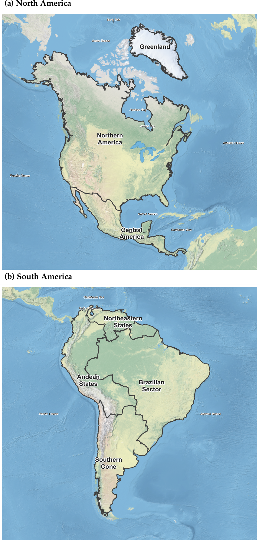
Figure 2.
Principal-landmass geographical units used in the Continental Atlas for (a) Africa and (b) Eurasia, with national boundaries from GADM (Version 4.1) [9] over a Natural Earth shaded-relief and bathymetric basemap [10]. The displayed geographical units represent the connected landmass configurations used for the continent-level fractal-dimension analysis.
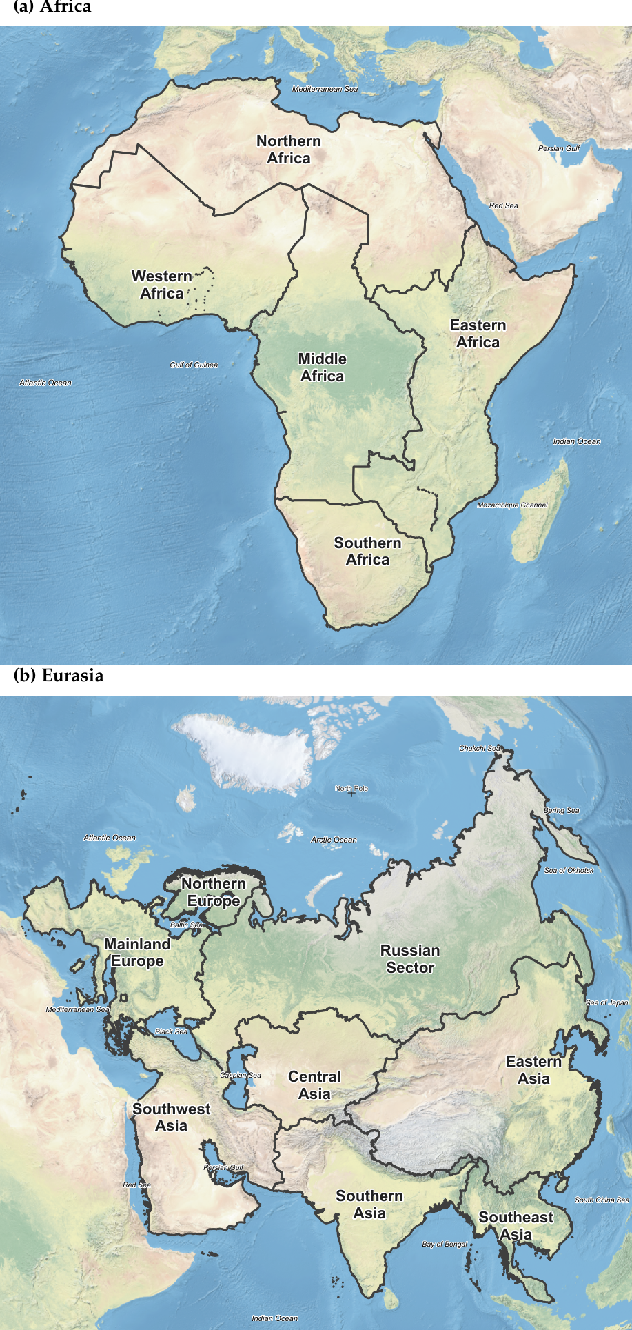
Figure 3.
Principal-landmass geographical units used in the Continental Atlas for (a) Oceania and (b) Antarctica, with national boundaries from GADM (Version 4.1) [9] over a Natural Earth shaded-relief and bathymetric basemap [10]. The displayed geographical units represent the connected landmass configurations used for the continent-level fractal-dimension analysis.
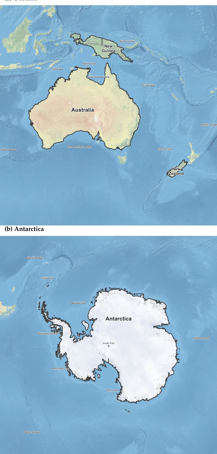
Figure 4.
Cross-method comparison of box-counting and divider fractal dimensions across six continents and 23 subcontinents. The dashed line denotes Symbol shape distinguishes geographic scale and grouping identifies the associated continental family.
Figure 4.
Cross-method comparison of box-counting and divider fractal dimensions across six continents and 23 subcontinents. The dashed line denotes Symbol shape distinguishes geographic scale and grouping identifies the associated continental family.
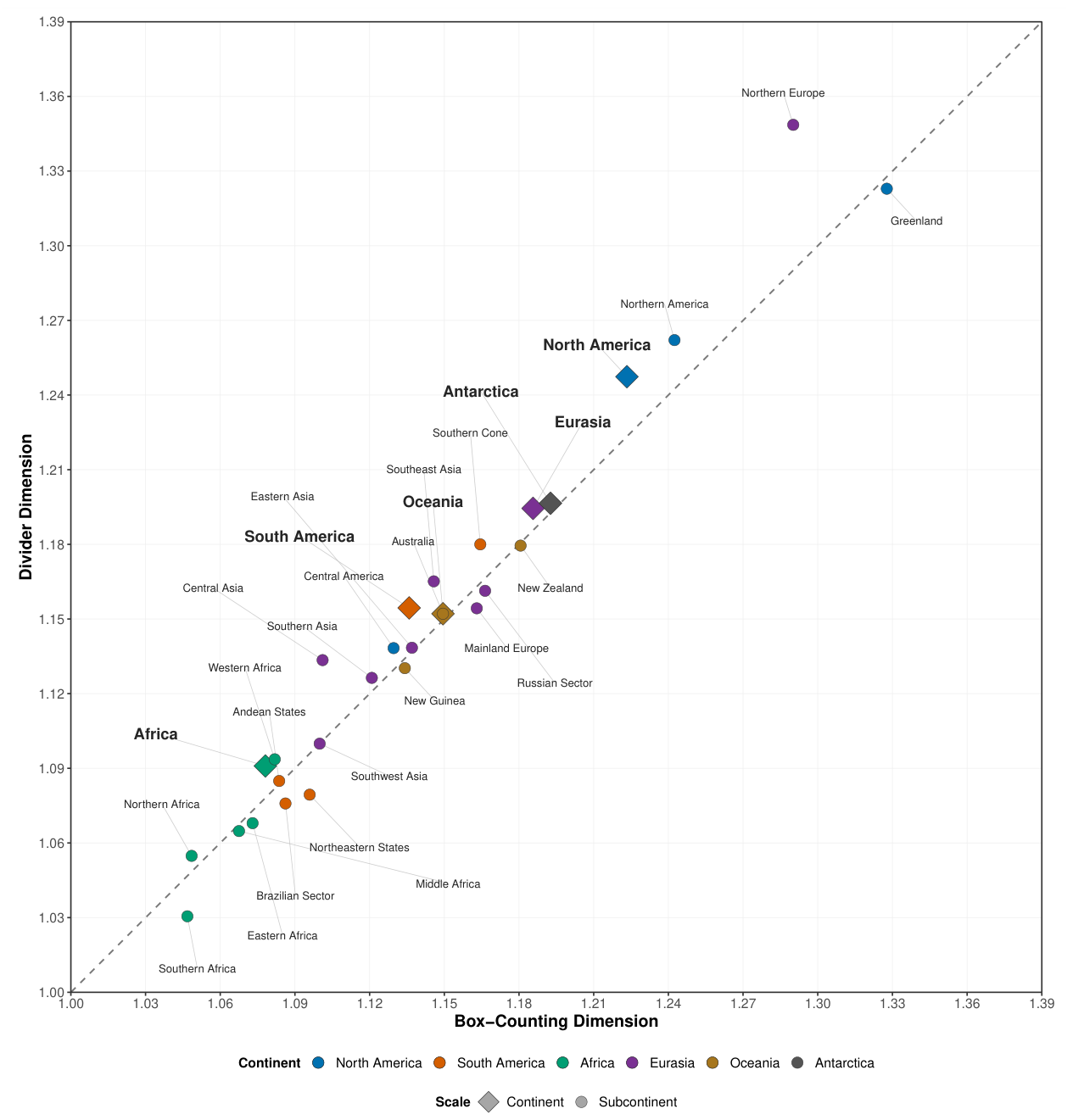
Figure 5.
Box-counting, divider, and equal-weight consensus fractal dimensions for six continents and 23 subcontinents, grouped by continental family. Parent units precede their associated subcontinental units.
Figure 5.
Box-counting, divider, and equal-weight consensus fractal dimensions for six continents and 23 subcontinents, grouped by continental family. Parent units precede their associated subcontinental units.
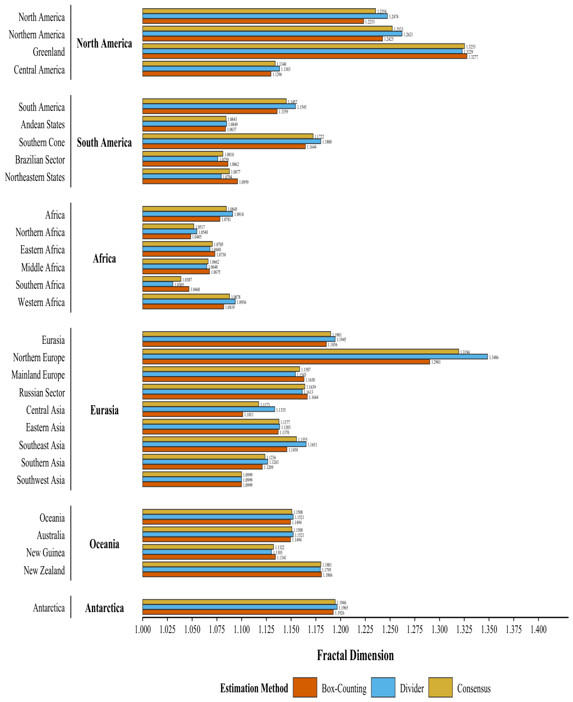

Table 1.
Study continental–subcontinental taxonomy, contributing countries or areas, source identifiers, and study-specific connectivity/exclusion rules (; ).
Table 1.
Study continental–subcontinental taxonomy, contributing countries or areas, source identifiers, and study-specific connectivity/exclusion rules (; ).
| # | Continent | Subcontinent | Geographic composition |
|---|---|---|---|
| 1 | North America | Northern America | Canada and USA [including Alaska]. |
| Greenland | Greenland. | ||
| Central America | Mexico, Belize, Costa Rica, El Salvador, Guatemala, Honduras, Nicaragua, and Panama. | ||
| 2 | South America | Andean States | Bolivia, Colombia, Ecuador, Peru. |
| Southern Cone | Argentina, Chile, Paraguay, Uruguay. | ||
| Brazilian Sector | Brazil. | ||
| Northeastern States | Venezuela, Guyana, Suriname, French Guiana. | ||
| 3 | Africa | Northern Africa | Algeria; Egypt [all of it]; Libya; Morocco; Sudan; Tunisia; Western Sahara [area]. |
| Eastern Africa | Burundi; Djibouti; Eritrea; Ethiopia; Kenya; Malawi; Mozambique; Rwanda; Somalia; South Sudan; Uganda; United Republic of Tanzania; Zambia; Zimbabwe. | ||
| Middle Africa | Angola; Cameroon; Central African Republic; Chad; Congo; Democratic Republic of the Congo; Equatorial Guinea [continental portion]; Gabon. | ||
| Southern Africa | Botswana; Eswatini; Lesotho; Namibia; South Africa. | ||
| Western Africa | Benin; Burkina Faso; Côte d’Ivoire; Gambia; Ghana; Guinea; Guinea-Bissau; Liberia; Mali; Mauritania; Niger; Nigeria; Senegal; Sierra Leone; Togo. | ||
| 4 | Eurasia | Northern Europe | Finland; Norway; Sweden. |
| Mainland Europe | Belarus; Bulgaria; Czechia; Estonia; Hungary; Latvia; Lithuania; Poland; Republic of Moldova; Romania; Slovakia; Ukraine; Kaliningrad; Albania; Bosnia and Herzegovina; Croatia; Greece; Holy City; Italy; Montenegro; North Macedonia; San Marino; Serbia; Slovenia; Andorra; Austria; Belgium; Denmark [mainland]; France [European mainland]; Germany; Gibraltar; Liechtenstein; Luxembourg; Monaco; Netherlands [European mainland]; Portugal; Spain; Switzerland. | ||
| Russian Sector | Russia [omitted Kaliningrad]. | ||
| Central Asia | Kazakhstan; Kyrgyzstan; Tajikistan; Turkmenistan; Uzbekistan. | ||
| Eastern Asia | China [including Hong Kong and Macao]; North Korea; Mongolia; South Korea. | ||
| Southeast Asia | Cambodia; Lao People’s Democratic Republic; Malaysia [peninsular portion]; Myanmar; Thailand; Viet Nam. | ||
| Southern Asia | Afghanistan; Bangladesh; Bhutan; India; Nepal; Pakistan. | ||
| Southwest Asia | Armenia; Azerbaijan; Georgia; Iran; Iraq; Israel; Jordan; Kuwait; Lebanon; Oman; Qatar; Saudi Arabia; Palestine; Syria; Türkiye [all of it]; United Arab Emirates; Yemen. | ||
| 5 | Oceania | Australia | Australia [Main Island]. |
| New Guinea | New Guinea [Entire Island]. | ||
| New Zealand | New Zealand [South Island]. | ||
| 6 | Antarctica | Antarctica | Antarctica. |
Table 2.
Scaling-window selection rules applied independently to each estimation method.
| Step | Selection rule |
|---|---|
| Candidate windows | Fit every contiguous interval containing at least six admissible scales. |
| Dimensional admissibility | Prefer windows yielding a geometrically plausible estimate, . |
| Near-optimal fit set | Let denote the largest adjusted coefficient of determination and retain
|
| Primary criterion | Within , maximize the logarithmic scale span
|
| Tie breaking | If required, prefer successively the window containing more retained scales and then the larger adjusted . |
| Diagnostic fallback | If no candidate satisfies , retain the closest diagnostic solution and flag the result rather than forcing dimensional admissibility. |
Table 3.
Fractal dimension estimations of the borders of 6 continents (mainlands) and 23 subcontinents (mainlands) using adaptive methods.
Table 3.
Fractal dimension estimations of the borders of 6 continents (mainlands) and 23 subcontinents (mainlands) using adaptive methods.
| # |
Geographic Unit |
Scale | Fractal Dimension and its Statistics | |||||
| Box-Counting | Divider | |||||||
|
Selected scale window (km) |
Selected scale window (km) |
|||||||
| 1 | North America | Continent | 1.223342 | 0.999967 | 5.8193–200.0000 | 1.247389 | 0.998317 | 5.8193–87.0123 |
| 1-1 | Northern America | Subcontinent | 1.242453 | 0.999948 | 4.9735–200.0000 | 1.262083 | 0.998484 | 4.9735–200.0000 |
| 1-2 | Greenland | Subcontinent | 1.327729 | 0.999657 | 1.6131–183.1275 | 1.322921 | 0.996238 | 8.5701–45.5316 |
| 1-3 | Central America | Subcontinent | 1.129626 | 0.999874 | 2.8030–200.0000 | 1.138308 | 0.998985 | 2.8030–73.2714 |
| 2 | South America | Continent | 1.135864 | 0.999903 | 5.0582–200.0000 | 1.154465 | 0.998305 | 5.0582–84.1894 |
| 2-1 | Andean States | Subcontinent | 1.083663 | 0.999935 | 2.6034–200.0000 | 1.084917 | 0.994933 | 9.3347–120.0076 |
| 2-2 | Southern Cone | Subcontinent | 1.164441 | 0.999955 | 2.2906–200.0000 | 1.180001 | 0.996580 | 2.9795–153.7621 |
| 2-3 | Brazilian Sector | Subcontinent | 1.086192 | 0.999977 | 3.5307–200.0000 | 1.075879 | 0.995946 | 4.4771–200.0000 |
| 2-4 | Northeastern States | Subcontinent | 1.095917 | 0.999801 | 1.4342–160.5253 | 1.079413 | 0.991181 | 4.3522–40.0788 |
| 3 | Africa | Continent | 1.078109 | 0.999937 | 6.3381–200.0000 | 1.090952 | 0.995627 | 6.3381–48.2797 |
| 3-1 | Northern Africa | Subcontinent | 1.048491 | 0.999960 | 3.4799–200.0000 | 1.054818 | 0.997525 | 23.4180–124.1751 |
| 3-2 | Eastern Africa | Subcontinent | 1.072987 | 0.999948 | 3.2704–200.0000 | 1.067961 | 0.998219 | 5.3060–123.2711 |
| 3-3 | Middle Africa | Subcontinent | 1.067525 | 0.999754 | 2.7854–200.0000 | 1.064794 | 0.997599 | 26.7640–94.0753 |
| 3-4 | Southern Africa | Subcontinent | 1.046781 | 0.999954 | 1.6830–200.0000 | 1.030536 | 0.990091 | 2.2291–200.0000 |
| 3-5 | Western Africa | Subcontinent | 1.081876 | 0.999917 | 2.4603–200.0000 | 1.093631 | 0.997121 | 4.1277–25.2458 |
| 4 | Eurasia | Continent | 1.185642 | 0.999926 | 8.6294–200.0000 | 1.194468 | 0.999384 | 8.6294–200.0000 |
| 4-1 | Northern Europe | Subcontinent | 1.290143 | 0.999760 | 1.2904–175.9368 | 1.348592 | 0.998583 | 4.1019–55.3462 |
| 4-2 | Mainland Europe | Subcontinent | 1.163024 | 0.999824 | 2.6365–200.0000 | 1.154305 | 0.997107 | 4.3873–43.4007 |
| 4-3 | Russian Sector | Subcontinent | 1.166369 | 0.999812 | 5.3572–200.0000 | 1.161340 | 0.997494 | 6.6285–130.6406 |
| 4-4 | Central Asia | Subcontinent | 1.101109 | 0.999785 | 2.1085–200.0000 | 1.133484 | 0.997550 | 13.7423–200.0000 |
| 4-5 | Eastern Asia | Subcontinent | 1.136995 | 0.999954 | 3.5264–200.0000 | 1.138454 | 0.998849 | 3.5264–200.0000 |
| 4-6 | Southeast Asia | Subcontinent | 1.145770 | 0.999945 | 1.9240–200.0000 | 1.165143 | 0.998194 | 2.5284–67.0632 |
| 4-7 | Southern Asia | Subcontinent | 1.120888 | 0.999954 | 2.8367–200.0000 | 1.126349 | 0.996190 | 3.6436–57.2055 |
| 4-8 | Southwest Asia | Subcontinent | 1.099926 | 0.999947 | 2.8162–200.0000 | 1.099913 | 0.997204 | 4.6502–200.0000 |
| 5 | Oceania | Continent | 1.149449 | 0.999880 | 2.9159–200.0000 | 1.152129 | 0.997222 | 2.9159–121.6184 |
| 5-1 | Australia | Subcontinent | 1.149449 | 0.999880 | 2.9159–200.0000 | 1.152129 | 0.997222 | 2.9159–121.6184 |
| 5-2 | New Guinea | Subcontinent | 1.134132 | 0.999835 | 1.3007–143.9255 | 1.130259 | 0.998380 | 1.7156–109.1203 |
| 5-3 | New Zealand | Subcontinent | 1.180630 | 0.999869 | 0.5395–79.7398 | 1.179499 | 0.995950 | 1.3028–13.6743 |
| 6 | Antarctica | Continent | 1.192644 | 0.999716 | 3.8820–200.0000 | 1.196504 | 0.997377 | 6.1725–200.0000 |
| Notes. denotes the estimated fractal dimension and the coefficient of determination. Estimates and are reported to six decimal places; selected scale windows (km), reported to four decimals, indicate the ranges retained for regression. | ||||||||
Table 4.
Scale-stratified descriptive statistics for continental and subcontinental boundary fractal dimensions ( continents; subcontinents).
Table 4.
Scale-stratified descriptive statistics for continental and subcontinental boundary fractal dimensions ( continents; subcontinents).
| Geographic scale | Method | Mean (SD) | Median [Q1, Q3] | Min–Max | PED0 (%) |
|---|---|---|---|---|---|
| Continent | Box counting | 1.160842 (0.051247) | 1.167546 [1.139261, 1.190893] | 1.078109–1.223342 | 16.08 |
| Divider | 1.172651 (0.053023) | 1.174467 [1.152713, 1.195995] | 1.090952–1.247389 | 17.27 | |
| Subcontinent | Box counting | 1.136353 (0.071797) | 1.129626 [1.084927, 1.163732] | 1.046781–1.327729 | 13.64 |
| Divider | 1.141075 (0.080180) | 1.133484 [1.082165, 1.163242] | 1.030536–1.348592 | 14.11 |
Notes. SD = sample standard deviation across the listed geographical units; Q1 and Q3 = first and third quartiles, respectively., the absolute percentage departure of the stratum mean from the linear benchmark D0 = 1. The PED0 (%) = 100 × continental set includes Antarctica. Oceania and Australia retain their respective continent and subcontinent observations
despite identical FD values. No pooled continent-plus-subcontinent mean is presented.
Table 5.
Cross-method agreement between box-counting and divider fractal-dimension estimates, evaluated separately by geographic scale( continents; subcontinents).
Table 5.
Cross-method agreement between box-counting and divider fractal-dimension estimates, evaluated separately by geographic scale( continents; subcontinents).
| Scale | Pearson r | Spearman | Lin CCC | Mean | Mean |
|---|---|---|---|---|---|
| Continent | 0.9876 | 0.9429 | 0.9624 | -0.011810 | 0.011810 |
| Subcontinent | 0.9822 | 0.9753 | 0.9743 | -0.004722 | 0.011191 |
Notes. Δ = DBC − DDIV, the paired box-counting minus divider fractal-dimension difference; Mean |Δ| is its mean absolute
value. Pearson r measures linear association, Spearman ρ measures rank association, and Lin CCC measures concordance
relative to the identity line. Coefficients describe only the selected units (six continents, including Antarctica; 23 subcontinents).
Oceania and Australia are retained separately in their respective geographic scales despite identical FD pairs.
Table 6.
Direct parent-continent fractal-dimension estimates and corresponding subcontinental summaries by continental family.
Table 6.
Direct parent-continent fractal-dimension estimates and corresponding subcontinental summaries by continental family.
| Continent | Subunits (m) |
Parent / | Subunit median / |
Subunit range / |
|---|---|---|---|---|
| North America | 3 | 1.223342 / 1.247389 | 1.242453 / 1.262083 | [1.129626–1.327729] / [1.138308–1.322921] |
| South America | 4 | 1.135864 / 1.154465 | 1.091055 / 1.082165 | [1.083663–1.164441] / [1.075879–1.180001] |
| Africa | 5 | 1.078109 / 1.090952 | 1.067525 / 1.064794 | [1.046781–1.081876] / [1.030536–1.093631] |
| Eurasia | 8 | 1.185642 / 1.194468 | 1.141383 / 1.146379 | [1.099926–1.290143] / [1.099913–1.348592] |
| Oceania | 3 | 1.149449 / 1.152129 | 1.149449 / 1.152129 | [1.134132–1.180630] / [1.130259–1.179499] |
| Antarctica | 0 | 1.192644 / 1.196504 | Not applicable | Not applicable |
Notes. = box-counting fractal dimension; = divider fractal dimension; m = number of subcontinents associated with each parent continent. Each parent FD is calculated from the complete parent boundary and is not computed from its subcontinental FD estimates. Subunit medians and ranges summarize only the associated subcontinents; each bracketed range displays the minimum–maximum within the specified method. Oceania and Australia share identical FD coordinates in the supplied dataset, but remain distinct continent and subcontinent records. Antarctica has no corresponding subcontinent records (), so its subunit median and range are not applicable. All FD values are shown to six decimal places.
Table 7.
Geographic units with the largest observed absolute cross-method differences between box-counting and divider fractal-dimension estimates.
Table 7.
Geographic units with the largest observed absolute cross-method differences between box-counting and divider fractal-dimension estimates.
| Geographic unit | Scale | ||||
|---|---|---|---|---|---|
| Northern Europe | Subcontinent | 1.290143 | 1.348592 | -0.058450 | 0.058450 |
| Central Asia | Subcontinent | 1.101109 | 1.133484 | -0.032375 | 0.032375 |
| North America | Continent | 1.223342 | 1.247389 | -0.024047 | 0.024047 |
| Northern America | Subcontinent | 1.242453 | 1.262083 | -0.019630 | 0.019630 |
Notes. DBC = box-counting fractal dimension; DDIV = divider fractal dimension. Δ = DBC − DDIV, and |Δ| is its absolute value.
Rows are sorted by decreasing |Δ|, with the sign of Δ retained. The six continental and 23 subcontinental estimates are distinct
geographical-scale records, not a random sample of independent units. Oceania and Australia have identical FD coordinates in
the source dataset but belong to different geographic scales; this numerical coincidence is not independent corroboration. The
table describes observed differences, not statistical significance or interchangeability of the methods. Interpretation should also
consider scaling-window diagnostics and source-geometry quality. FD results are displayed to six decimal places.
Table 8.
Geographical Unit box-counting, divider, and consensus fractal dimensions, grouped by scale and measurement method ().
Table 8.
Geographical Unit box-counting, divider, and consensus fractal dimensions, grouped by scale and measurement method ().
| Geographic Unit | Scale | Geographic Unit | Scale | ||||||
|---|---|---|---|---|---|---|---|---|---|
| North America | Continent | 1.223342 | 1.247389 | 1.235365 | Northern America | Subcontinent | 1.242453 | 1.262083 | 1.252268 |
| Greenland | Subcontinent | 1.327729 | 1.322921 | 1.325325 | Central America | Subcontinent | 1.129626 | 1.138308 | 1.133967 |
| South America | |||||||||
| South America | Continent | 1.135864 | 1.154465 | 1.145164 | Andean States | Subcontinent | 1.083663 | 1.084917 | 1.084290 |
| Southern Cone | Subcontinent | 1.164441 | 1.180001 | 1.172221 | Brazilian Sector | Subcontinent | 1.086192 | 1.075879 | 1.081035 |
| Northeastern States | Subcontinent | 1.095917 | 1.079413 | 1.087665 | |||||
| Africa | |||||||||
| Africa | Continent | 1.078109 | 1.090952 | 1.084530 | Northern Africa | Subcontinent | 1.048491 | 1.054818 | 1.051655 |
| Eastern Africa | Subcontinent | 1.072987 | 1.067961 | 1.070474 | Middle Africa | Subcontinent | 1.067525 | 1.064794 | 1.066160 |
| Southern Africa | Subcontinent | 1.046781 | 1.030536 | 1.038658 | Western Africa | Subcontinent | 1.081876 | 1.093631 | 1.087754 |
| Eurasia | |||||||||
| Eurasia | Continent | 1.185642 | 1.194468 | 1.190055 | Northern Europe | Subcontinent | 1.290143 | 1.348592 | 1.319368 |
| Mainland Europe | Subcontinent | 1.163024 | 1.154305 | 1.158665 | Russian Sector | Subcontinent | 1.166369 | 1.161340 | 1.163855 |
| Central Asia | Subcontinent | 1.101109 | 1.133484 | 1.117296 | Eastern Asia | Subcontinent | 1.136995 | 1.138454 | 1.137725 |
| Southeast Asia | Subcontinent | 1.145770 | 1.165143 | 1.155457 | Southern Asia | Subcontinent | 1.120888 | 1.126349 | 1.123619 |
| Southwest Asia | Subcontinent | 1.099926 | 1.099913 | 1.099919 | |||||
| Oceania | |||||||||
| Oceania | Continent | 1.149449 | 1.152129 | 1.150789 | Australia | Subcontinent | 1.149449 | 1.152129 | 1.150789 |
| New Guinea | Subcontinent | 1.134132 | 1.130259 | 1.132196 | New Zealand | Subcontinent | 1.180630 | 1.179499 | 1.180065 |
| Antarctica | |||||||||
| Antarctica | Continent | 1.192644 | 1.196504 | 1.194574 | |||||
Notes. = box-counting fractal dimension; = divider fractal dimension; and . All consensus values are calculated separately for each geographic unit using full-precision source estimates; only displayed values are rounded to six decimal places. Each continent is placed immediately before its constituent subcontinents. The continent estimates are direct boundary measurements, not averages of their subcontinents. Oceania and Australia retain distinct geographic-scale rows but have identical paired FD and consensus values in the source dataset. Antarctica has no corresponding subcontinent row.
Disclaimer/Publisher’s Note: The statements, opinions and data contained in all publications are solely those of the individual author(s) and contributor(s) and not of MDPI and/or the editor(s). MDPI and/or the editor(s) disclaim responsibility for any injury to people or property resulting from any ideas, methods, instructions or products referred to in the content. |
© 2026 by the authors. Licensee MDPI, Basel, Switzerland. This article is an open access article distributed under the terms and conditions of the Creative Commons Attribution (CC BY) license (http://creativecommons.org/licenses/by/4.0/).
Copyright: This open access article is published under a Creative Commons CC BY 4.0 license, which permit the free download, distribution, and reuse, provided that the author and preprint are cited in any reuse.