

Submitted:
02 October 2026
Posted:
06 October 2026
You are already at the latest version
Abstract
Atlantic salmon aquaculture faces persistent welfare challenges from handling, confinement, disease and delousing, yet established welfare indicators typically require capture or invasive sampling and signal problems only after they have developed. Melanin-based pigmentation in salmonids is associated with stress responsiveness, but quantitative methods for measuring stress-associated fading of individual spots are lacking, and longitudinal photometry in repeatedly imaged individuals is vulnerable to between-session drift in illumination and camera settings. We present a computer vision framework that quantifies opercular melanin spots while explicitly controlling for image acquisition. Opercular regions were detected with YOLOv8, registered by projective transformation, and spots segmented with point-prompted fine-tuned SAM 2 model. Images were linearized and normalized to a common sensor exposure using EXIF metadata prior to feature extraction, and all effects were further adjusted for residual per-image exposure differences. Twenty-one salmon were imaged before and after 18 h confinement (676 matched spot pairs); plasma cortisol confirmed the challenge (W=14, p < 0.001). Eight control fish were imaged once as a reference group. Confinement was associated with increased spot grayscale intensity, reduced spot-to-background contrast and reduced spot area, with closely matching estimates on both opercula. Control fish were indistinguishable from pre-stress fish in contrast (p=0.28) but differed markedly from post-stress fish (d=1.04, p=0.002). Since control fish were imaged at a single timepoint, elapsed time cannot be excluded as a contributor. The framework provides a photometrically controlled, non-invasive basis for quantifying pigmentation dynamics in salmon.
Keywords:
salmo salar
; fish welfare
; precision aquaculture
; melanin pigmentation
; image segmentation
; photometric normalization
; non-invasive stress indicator
; confinement stress
1. Introduction
The aquaculture industry is currently challenged by extraordinarily high Atlantic salmon mortality, which has intensified the search for new welfare indicators and management practices capable of reducing these losses. In 2024, 45.8 million salmon were reported to have died during land-based hatchery production, and a further 57.8 million during the marine phase, largely from injuries sustained during delousing, complex gill disease, and winter ulcers [42]. Salmon aquaculture is frequently characterized by adverse conditions, including disease outbreaks and routine management procedures such as delousing and handling [48,52,61]. Growing recognition of how these stressors affect fish welfare has stimulated considerable scholarly interest in advanced methodologies for assessing welfare across diverse production systems [1,25].
Operational welfare indicators for farmed Atlantic salmon are well established [46], but the most informative of them share two limitations. Physiological indicators such as plasma cortisol require capture, restraint and blood sampling, procedures that themselves elicit a stress response, and which can therefore be applied only to a small subset of animals at discrete timepoints [15,57]. Morphological indicators such as fin damage, scale loss and ulceration are non-invasive, but they register damage only after it has occurred. Neither class supports continuous, individual-level monitoring of physiological state. As the industry expands, more sophisticated technologies are required to monitor fish farms in line with the precision livestock farming concept [7]. One under-researched avenue is the assessment of visual traits using artificial intelligence [44,67], and in particular of melanin-based spots on the salmon body [19,39,63].
The bodies of Atlantic salmon are covered with black spots formed by aggregations of chromatophores, principally melanophores, which produce and store melanin. Melanin is primarily a light-absorbing pigment that serves diverse ecological functions in vertebrates, including photoprotection, camouflage and communication [11,21,34,40,53,54]. Its functions in fish are likely equally diverse but have been studied less extensively. Nevertheless, previous work indicates that the number of melanin spots on salmonid fish carries information about individual physiology and behavior. In strains of Atlantic salmon (Salmo salar) and rainbow trout (Oncorhynchus mykiss), individuals with more spots exhibited a reduced cortisol response to stress, recovered feed intake more rapidly after transfer to a novel environment, and harbored fewer female egg-bearing ectoparasites such as sea lice [26,29,30].
Melanin signalling may therefore serve as a non-invasive indicator of stress and welfare in Atlantic salmon, and two endocrine pathways provide a mechanistic basis for stress-induced fading. The first involves melanin-concentrating hormone (MCH). MCH does not bind the Gs-protein-coupled melanocortin receptors (MC1–MC5), among which MC1 primarily regulates pigmentation [38]; instead, it binds selectively to the Gi-protein-coupled receptor MCH-R1 [24,65]. Receptor binding inhibits adenylyl cyclase and thereby suppresses the conversion of adenosine triphosphate (ATP) to cyclic adenosine monophosphate (cAMP) [17,58]. Reduced cAMP causes melanosomes to aggregate toward the center of the melanophore rather than disperse throughout its dendrites, exposing the underlying iridophores and causing the skin to appear paler. This mechanism operates over seconds to minutes and is readily reversible [45].
The second pathway involves agouti signalling protein (ASP), an antagonist of alpha-melanocyte-stimulating hormone (α-MSH), the hormone that normally promotes melanosome dispersion [9,37]. Under stressful conditions, elevated plasma cortisol increases ASP expression [10,26,37]. Binding of ASP to MC1 receptors prevents activation of adenylyl cyclase and halts cAMP production, again reducing melanosome dispersion. Unlike MCH-mediated translocation, ASP acts transcriptionally and therefore over hours to days [62]. The two pathways make partially distinguishable predictions: rapid melanosome aggregation should alter spot intensity while leaving spot boundaries largely intact, whereas sustained suppression of melanin dispersion should also erode spot margins.
Testing these predictions requires measuring the appearance of the same spots, on the same fish, at more than one timepoint and this is where the principal methodological obstacle lies. Photometric measurement of individual animals is acutely sensitive to image acquisition. Between-session differences in illumination, camera exposure, viewing geometry and working distance produce changes in recorded pixel intensity that are, in the resulting images, indistinguishable from genuine changes in pigmentation. A camera operating in automatic exposure mode varies its settings from frame to frame in response to scene composition, and consumer image formats apply a non-linear transfer function that renders pixel values non-proportional to scene radiance. The study of animal coloration has long recognized this problem and addressed it through calibrated photography [59,64], but such calibration has not been applied to melanin spot quantification in salmonids. Without it, a reported reduction in spot contrast cannot be confidently attributed to the animal rather than to the instrument.
In our previous studies [20,31] we presented a pipeline for detecting, registering and segmenting melanin-based opercular spots, and reported as proof of principle that spot grayscale intensity shifts toward pigmentation fading following a confinement episode. Gunnes et al. [20] further associated the quantified fading with regional variation in serotonin transmission in Atlantic salmon. Both studies were framed as demonstrations that image-based methods can detect temporal change in opercular spots, rather than as quantifications of the effect, and neither examined image acquisition as a source of that change. The photographs were taken with a consumer camera in automatic exposure mode, in a booth open at the front to ambient daylight, and the resulting exposure settings varied by up to 2.7 stops between paired images of the same individual, variation that alters recorded pixel intensity independently of pigmentation and that is not removed by geometric registration or spatial illumination correction.
The present study addresses this directly. We introduce a photometric normalization procedure that linearizes images through the inverse sRGB transfer function and rescales them to a common sensor exposure derived from EXIF metadata, carry residual per-image exposure differences into the statistical models as covariates, and extend the feature set beyond spot intensity to local background intensity, spot-to-background contrast computed in linear light, and spot area. This allows the effect to be reported as an exposure-adjusted estimate with confidence intervals rather than as a demonstration of detectability. The imaging dataset, the confinement protocol and the trained detection and segmentation models are shared between the two studies; the photometric normalization procedure, the extended feature set, the exposure-adjusted statistical framework and all results reported here are new.
On this basis, we hypothesized that confinement stress produces measurable, spot-specific fading that can be distinguished from variation introduced during image acquisition.
The contributions of this work are as follows:
- -
- A photometric normalization procedure for longitudinal fish imaging. Images are linearized through the inverse sRGB transfer function and normalized to a common sensor exposure computed from EXIF metadata, placing photographs acquired under automatic exposure on a common radiometric scale. In the present dataset this removed exposure differences of up to 2.7 stops between paired images of the same individuals.
- -
- A per-spot feature set that operationalizes fading as a measurable quantity. Spot intensity, local background intensity, spot-to-background contrast computed in linear light, and spot area are extracted for each individually matched spot, replacing qualitative assessment of pigmentation change with quantities that can be compared across sessions.
- -
- An exposure-adjusted statistical framework. Residual per-image exposure differences are carried into the statistical models as covariates, so that reported effects estimate the change expected at zero exposure difference rather than the raw session-to-session change. This distinguishes biological signals from residual instrument variation.
- -
- A quantitative test of whether opercular spot responds to confinement. Twenty-one Atlantic salmon were imaged before and after an 18 h confinement challenge, yielding 676 individually matched spot pairs, with plasma cortisol confirming the physiological response; eight control fish were imaged as a reference group.
- -
- An open-source implementation, including model weights and per-image acquisition metadata, enabling replication on independent stocks and facilities.
2. Related Work
2.1. Computer Vision Applied to Melanin Spots in Salmonids
Work applying computer vision to melanin spots in Atlantic salmon has concentrated almost entirely on melanized discoloration in the fillet rather than on the skin of live fish [41,69]. This emphasis follows from the commercial context. Melanin spots in fillets are a downgrading defect with direct economic consequence, and the imaging conditions on a processing line are controlled and repeatable: a stationary subject, fixed working distance, and uniform illumination. Broader reviews of machine vision in aquaculture report the same pattern, documenting extensive application to biomass estimation, species identification and quality grading, but comparatively little to pigmentation on living animals [56]. The consequence is that the existing literature measures pigmentation at a single terminal timepoint, post-mortem, and at the level of the whole fillet. It offers no basis for tracking an individual spot on a living fish over time, which is the measurement a welfare indicator requires.
2.2. Deep Learning for Fish Monitoring, Disease Detection and Re-Identification
A second and larger body of work applies detection and classification models to monitoring tasks in aquaculture. Ahmed et al. [2] combined image processing, hand-crafted feature engineering and classical machine learning to identify disease-infected salmon, and Gupta et al. [18] trained a convolutional neural network to classify wounds and lice infestation under varying lighting conditions. Object detectors have been applied widely to counting and surveillance: Banno et al. [4] used YOLOv4 to count wild fish around sea cages, Yu et al. [68] modified the YOLOv5 architecture for lateral line detection, and Ranjan et al. [50] combined YOLOv7 with edge computing and IoT infrastructure for real-time mortality monitoring in tanks.
Most relevant to the present work is the re-identification literature, which establishes the premise on which our design depends. Cisar et al. [12] re-identified individual salmon across images acquired on different dates, using a convolutional neural network for short-term identification and histogram-of-oriented-gradient features for long-term identification. Bekkozhayeva et al. [5] achieved comparable performance using body scale patterns. Zhou et al. [70] re-identified brook trout through a four-stage pipeline: region-of-interest extraction with Faster R-CNN, foreground and pigmentation-pattern extraction by morphological and spectral filtering, feature encoding with a deep residual network, and matching by cosine similarity.
The significance of these studies for the present work is that they demonstrate melanin spot patterns to be individually distinctive and temporally stable, stable enough to serve as a biometric key across months. We exploit that stability differently. Rather than using the pattern to establish identity, we treat each matched spot as a repeated measure and ask whether its appearance changes. This distinction carries a methodological consequence that is easily overlooked. Re-identification is largely invariant to photometric variation, because the identity signal resides in spot geometry and topology rather than in absolute intensity; a re-identification pipeline will succeed on images that differ substantially in exposure and illumination. The demonstrated success of these methods therefore provides no assurance that intensity measurements extracted from the same images are comparable across sessions. Photometric measurement imposes requirements that re-identification does not.
2.3. Calibrated Photography for Quantitative Color Measurement
Quantitative measurement of animal coloration from digital photographs is a mature methodology with a well-developed treatment of precisely the problems that arise here. Stevens et al. [59] set out step-by-step guidelines for obtaining accurate data from digital cameras, observing that many studies employing digital photography are unaware of critical acquisition issues, particularly the non-linearity of camera response to light intensity. Their procedure requires linearizing the camera response, equalizing color channels against reflectance standards, and mapping camera color space to a target space. Akkaynak et al. [3] formalized the processing chain for commercial off-the-shelf cameras and demonstrated applications across biomedical engineering, artwork photography, marine biology and underwater imaging; they state the precondition explicitly, namely that such cameras yield quantitative data only if images are captured in raw format and processed so as to preserve a linear relationship with scene radiance. Troscianko and Stevens [64] implemented these steps in a freely available toolbox that generates radiance-linear images from the raw files of numerous camera brands, normalizes them against in-frame grey standards, and additionally requires that images be rescaled to a common number of pixels per unit length before patterns are compared across photographs. These methods define the standard for quantitative color measurement, and they share two preconditions that are difficult to satisfy in an aquaculture setting. First, they require raw sensor data. Second, they require a physical reflectance standard within the frame of every photograph.
Imaging in a research or production facility is performed on wet, mobile animals under time pressure, frequently with a rugged compact camera operating in automatic exposure mode and writing only compressed output. Under these conditions the camera selects its own exposure in response to scene composition, and the in-camera pipeline applies a non-linear transfer function and tone curve before the file is written [27], so that recorded pixel values bear no fixed relationship to scene radiance. Neither precondition can be satisfied retrospectively. Existing image archives, including our own, therefore fall outside the scope of these established methods, and the pigmentation literature in salmonids has consequently proceeded without photometric control of any kind.
The present study addresses this gap by substituting an analytically recoverable radiometric reference for a physical one. Exposure metadata recorded in the EXIF header of every consumer image file: shutter speed, aperture and sensitivity, fully determines the sensor exposure applied to the scene. Inverting the standard sRGB transfer function and dividing by this exposure factor places images acquired under automatic exposure onto a common relative radiometric scale, without raw data and without a calibration target. Applied to the present dataset, this procedure removed exposure differences of up to 2.7 stops between paired images of the same individual.
We regard this as complementary to calibrated photography rather than a replacement for it. The procedure recovers relative exposure, not absolute reflectance, and cannot correct for changes in scene illumination, in spectral composition, or in camera-specific tone curves that depart from the sRGB standard. Two safeguards follow from this limitation. Residual per-image exposure differences are carried into the statistical models as covariates, so that reported effects estimate the change expected at zero exposure difference. And, following the image-scaling requirement identified by Troscianko and Stevens [64], between-group comparisons are restricted to features invariant to image scale, since our reference-group images were acquired at a different working distance.
2.4. Positioning
Our methodology draws on the fish detection and re-identification literature, employing an object detector for opercular region localization and a promptable transformer-based segmentation model for spot delineation within the detected regions [31,32]. It departs from that literature in what it measures, and in how the validity of the measurement is established. Where prior work on salmonid melanin spots measures pigmentation post-mortem in the fillet, we measure it on whole fish, in situ on the operculum. Where re-identification work treats spot patterns as a stable identity signal, we treat individual spots as repeated measures of a changing physiological state. And where both bodies of work take image intensity at face value, we make the recovery of comparable intensity across imaging sessions an explicit and validated component of the method. Table 1 summarizes this positioning.
The objective of this study is to quantify fading in melanin-based opercular spots in Atlantic salmon from photometrically normalized images, and to evaluate whether such fading constitutes a candidate non-invasive indicator of stress and welfare.
3. Materials and Methods
The methodology consists of a photometrically normalized pipeline for quantifying individual melanin-based opercular spots in Atlantic salmon images acquired before and after a standardized stressor. Opercular regions were first detected using a YOLOv8 detector [23] and subsequently cropped. The resulting crops were linearized using the inverse sRGB transfer function and normalized by the sensor exposure derived from the EXIF metadata. A grayscale adaptation of Retinex [33,49] normalization was then applied to correct for residual spatial illumination non-uniformity. Corresponding opercula from the two imaging sessions were matched through projective registration. Individual spots within the registered opercula were subsequently detected and matched across sessions, and fine-grained spot masks were generated using a point-prompted, fine-tuned Segment Anything Model 2 [51]. Finally, photometric and morphological features were extracted from the spot masks in linear light, while the residual per-image exposure was included as a covariate in the statistical models. The complete pipeline is illustrated in Figure 1. The imaging dataset, confinement protocol, and trained models are shared with our previous study [31]; however, the photometric normalization procedure, feature set, statistical framework, and all results presented here are novel.
3.1. Dataset
The dataset was the same as described in our previous study [31] and was collected at the Institute of Marine Research (IMR), Matre Research Centre, Norway. It included images of 130 Atlantic salmon, approximately 2.2 years of mean age and weighing 2–10 kg, photographed using an Olympus TG-6 camera (Olympus Corporation, Tokyo, Japan) with automatic camera settings against a blue background. All fish were netted from the holding tank and anaesthetised before photography. Reference fish (n = 8) and fish photographed after confinement received a lethal dose of MS-222, whereas the pre-confinement images were acquired under sedation. Fish were photographed immediately after removal from the anaesthetic bath. The full husbandry and anaesthesia protocol is reported in Laique et al. [31]. The original dataset included both head and body images. In the present study, only 520 close-up head images were used because the operculum regions and the enclosed melanin-based spots were clearly visible. Representative left- and right-side close-up head images are shown in Figure 2.
3.2. Annotations
Annotation followed the protocol established in our previous study [31] and is summarized here for completeness. Operculum and spot regions were annotated in 275 close-up head images using Roboflow's annotation toolkit [14] by a single annotator (TL), with annotations reviewed and agreed by the supervisory team at scheduled project meetings. Spots were annotated as polygons under an instance-segmentation strategy to accommodate variation in spot size, shape and texture, yielding 275 operculum regions and approximately 9,000 enclosed spots. Images were partitioned into training, validation and test sets in an approximate 70:20:10 ratio (193, 55 and 27 images, respectively), and geometric and pixel-intensity augmentations were applied to the training images to increase variation [66], expanding the training set to 1,065 images representing approximately 35,000 spot instances. Because individual fish contributed multiple images, partitioning was performed at the image level and fish-level independence between subsets was not enforced; the reported detection and segmentation metrics should therefore be interpreted as within-population performance rather than as generalization to entirely unseen individuals. The 100 close-up head images used for downstream analysis (8 control, 21 stressed fish) were held out entirely from model development and used only at the inference stage. Examples of annotated spots and operculum region are shown in Figure 3.
3.3. Segmentation Models
Three computer vision models were used in the segmentation pipeline. YOLOv8-seg [23] was used for both operculum identification and spot segmentation. To refine the spot masks, YOLO-derived spot predictions were converted into bounding boxes and point prompts, which were then provided together with the corresponding operculum image to a fine-tuned Segment Anything Model 2.1 (SAM 2.1) [51].
3.3.1. Fine-Tuning and Validation of Models
The YOLOv8x-seg model, comprising 68.2 million parameters, was fine-tuned separately on the operculum and spot datasets. Segment Anything Model 2 (SAM 2.1) was fine-tuned on the spot dataset. The YOLOv8x-seg models were fine-tuned and evaluated using the Ultralytics library [23], and SAM 2.1 using the official SAM 2 training code (Ravi et al., 2024). Fine-tuning and evaluation were performed in Google Colab on an NVIDIA A100 GPU with 40 GB of memory. Inference was conducted locally on an NVIDIA RTX 3500 Ada Generation GPU in an Anaconda3 environment (version 2024.02-1) configured with Python 3.10.14, PyTorch 2.8.0, CUDA 12.6 and Ultralytics 8.4.56.
3.3.2. Yolov8 for Operculum
A YOLOv8-seg model pretrained on the COCO dataset [35] was fine-tuned for operculum segmentation on the 275 annotated operculum images using the Ultralytics framework [23]. Training hyperparameters are given in Table 2. Regularization was applied through dropout and early stopping, halting training when validation performance had not improved for 25 consecutive epochs. Augmentations were applied on-the-fly during training via the Albumentations library [8] and included Gaussian blur, contrast-limited adaptive histogram equalization, grayscale conversion and tile-size adjustment. The photometric augmentations are of particular relevance here, as they reduce the sensitivity of the trained model to the between-session exposure variation. Model performance was evaluated using precision, recall and mean average precision (mAP), defined below. Quantitative results are presented in Table 3 and training and validation loss curves in Figure 4.
where TP, FP, and FN represent true positives, false positives, and false negatives, respectively. Recall describes the proportion of true objects detected by the model, whereas precision describes the proportion of model detections that were correct. C is the number of classes, and T denotes the set of confidence or IoU thresholds used to compute average precision.
3.3.3. Yolov8 for Spots
A pretrained YOLOv8-seg model was fine-tuned for spot localization on the augmented spot dataset using the Ultralytics segmentation framework [23]. Training configuration was identical to that used for the operculum model (Table 2). Quantitative performance metrics for the spot-localization model are presented in Table 4, and training and validation loss curves in Figure 5.
3.3.4. Segment Anything Model 2.1 for Spot-Mask Refinement
SAM 2.1 was fine-tuned from the pretrained Hiera-B+ checkpoint [51,55] on the augmented spot dataset. The image encoder, memory attention module and memory encoder were optimized with AdamW under mixed precision, using a cosine learning-rate schedule and layer-wise decay; the image encoder was assigned a lower base learning rate than the remaining modules to preserve the pretrained representation. The training objective combined mask, Dice, IoU and object-classification losses, with the mask term weighted most strongly [51]. Point and box prompts were sampled with equal probability during training, so that the model adapted to both prompt types produced by the upstream detector. The full training configuration is given in Table 5 and training loss curves are shown in Figure 6. The fine-tuned model was validated on a held-out test set and the Intersection-over-union (IoU) and Dice similarity coefficient (DICE) metrics separated by prompt type are mentioned in Table 6.
Where A is the set of pixels in predicted segmentation mask, B is the set of pixels in the ground-truth mask, is number of pixels in both masks (TP), is number of pixels in either mask (TP+FP+FN), |A|, |B| are pixel counts of the predicted and ground-truth masks respectively.
3.3.5. Comparison with Intensity Thresholding Methods
The spots are darker than the surrounding opercular skin, so the SAM 2-based method was additionally benchmarked against two classical intensity-thresholding baselines: global Otsu thresholding [47] and local adaptive (Gaussian-weighted mean) thresholding, both implemented in OpenCV [6]. A single threshold applied to the full 1080 × 1080 image is uninformative for this task, because the image-level intensity histogram is dominated by skin rather than by spot-to-background contrast. Each baseline was therefore given the same spatial prior as the SAM bounding-box prompt, thresholding a crop padded around each instance's annotated bounding box by max (6 px, 0.4 × the longer bounding-box side). Within each crop, Otsu selected a single data-driven threshold from the crop's bimodal intensity histogram, and the adaptive method thresholded each pixel against a Gaussian-weighted local mean (block size 60% of the crop's shorter side, offset C = 2); both were inverted to select the darker mode. Where thresholding yielded more than one connected foreground component, for example when a neighboring spot fell inside the padded crop, the component nearest the bounding-box center was retained as the predicted mask and mapped back to full-image coordinates; if no foreground component survived, the predicted mask was empty. This gives both baselines the same localization information as the SAM box prompt, isolating the comparison to segmentation quality rather than localization. Both methods were scored on the same set of 832 spot instances; IoU and Dice values are reported in Table 6.
3.4. Inference Workflow
The inference workflow extends that reported in our previous study [31] by inserting a photometric normalization stage between operculum extraction and all subsequent stages. This ordering is deliberate: every downstream quantity, spot intensity, background intensity, contrast and area, is derived from pixel values, and those values must be placed on a common radiometric scale before they can be compared across imaging sessions. The complete workflow comprises six stages: (1) operculum extraction, (2) photometric normalization, (3) Retinex normalization, (4) projective registration, (5) spot segmentation, and (6) spot matching and feature extraction. The workflow is illustrated in Figure 1.
3.4.1. Operculum Extraction
Left and right opercular regions were localized in each close-up head image using the fine-tuned YOLOv8-seg operculum model. The predicted mask was used to crop the opercular region, which formed the input to all subsequent stages.
3.4.2. Photometric Normalization
Images were acquired with a consumer compact camera operating in program auto-exposure mode. Under this mode the camera selects shutter speed in response to scene composition, so that two photographs of the same subject taken in different sessions may be exposed differently even when illumination is unchanged. In addition, the camera writes gamma-encoded sRGB output, in which recorded pixel values are a non-linear function of scene radiance [27]. Neither effect is corrected by geometric registration or by spatial illumination correction, and both directly bias photometric measurement. Photometric normalization therefore proceeds in three steps: linearization, exposure normalization, and re-encoding.
- Linearization: Each 8-bit channel value V ∈ [0,255] was scaled to v = V/255 and mapped to relative scene radiance by the inverse sRGB electro-optical transfer function:
This inverts the encoding applied in-camera and yields values proportional to the light captured by the sensor.
- Exposure normalization: The sensor exposure applied to each image is fully determined by the acquisition settings recorded in its EXIF header. For shutter speed t(seconds), f-number N, and sensitivity S(ISO), the relative exposure is
Since the recorded radiance of a surface of luminance Lscene is proportional to Lscene ⋅ H, dividing by Hrecovers a quantity proportional to scene luminance alone. Each image was therefore rescaled to a common reference exposure Href:
where Href is the median exposure across the full image set. The choice of Href is arbitrary and affects only the absolute scale of the output.
- Re-encoding: To retain precision in the dark spot interiors under 8-bit storage, and to preserve compatibility with the downstream segmentation models, normalized images were re-encoded using the forward sRGB transfer function after division by a single global scale factor Σ:
Σ was defined as the maximum, across all images, of the 99.9th percentile of Lrel, ensuring that no image clipped. As with Href, Σ was computed once over the entire dataset, including both stressed and reference animals, and applied identically to every image. All photometric features were subsequently computed after re-linearization by Eq. (6) and multiplication by Σ, so that measurements were made in linear light rather than on gamma-encoded values.
In the present dataset, exposure differed by up to 2.7 stops between paired images of the same individual, with a within-session standard deviation of approximately 0.8 stops
3.4.3. Retinex Normalization
Residual spatial non-uniformity in illumination was reduced using the grayscale adaptation of white-patch Retinex algorithm reported in Laique et al. [31], applied here after photometric normalization. The procedure performs a two-point affine correction of the luminance channel using reference regions present in the frame of every photograph. Eye and ID-tag regions were annotated using the smart polygon tool in Roboflow [14]. Within the segmented eye region, pixels were sorted in ascending order of intensity and the darkest 20% averaged to give a black reference β; within the segmented ID-tag region, pixels were sorted in descending order and the brightest 20% averaged to give a white reference, from which the contrast scaling α was derived. Each opercular region was converted to CIELAB colour space, and the luminance channel corrected as
The corrected luminance channel was then recombined with the unmodified a*and b*channels and converted back to RGB.
3.4.4. Projective Registration:
Extracted opercular regions were sorted into pre- and post-stress groups and registered side-wise, so that each operculum of a given individual at the pre-stress session was aligned to corresponding operculum of the same individual post-stress, left to left and right to right. Registration establishes the spatial correspondence required for spot-level pairing and follows the procedure reported in Laique et al. [31], implemented with OpenCV [6]:
- Pre- and post-stress opercular regions were converted to grayscale.
- Keypoints and descriptors were detected using the scale-invariant feature transform, SIFT [36](Lowe, 2004).
- Descriptors were matched using a FLANN-based approximate nearest-neighbour matcher [43].
- Lowe's ratio test [36] was applied to retain only unambiguous correspondences.
- The homography was applied to the pre-stress region to align it with its post-stress counterpart.
3.4.5. Spot Segmentation
Spots were detected within each registered, normalized opercular region using the fine-tuned YOLOv8-seg spot model. Predicted spot masks were converted to bounding boxes, and box centers taken as point prompts. Boxes and point prompts were supplied together with the corresponding opercular image to the fine-tuned SAM 2.1 model, which returned refined per-spot segmentation masks. The spot segmentation stages can be seen in Figure 7.
3.4.6. Spot Matching, Curation and Feature Extraction
Corresponding spots were paired across sessions by nearest-neighbor matching of mask centroids in the registered coordinate frame, using Euclidean distance. Spots without an acceptable match in the paired image were excluded from the paired analysis.
Matched spots were then manually curated. Spots obscured by mucus, affected by specular reflection, or partially occluded were removed prior to feature extraction. Curation was performed on the registered image pairs.
For each retained spot, the following features were computed in linear light:
- Spot intensity: the mean luminance of pixels within the SAM 2.1 mask.
- Background intensity: the mean luminance of an annulus formed by dilating the spot polygon to 1.5× its original extent and subtracting the spot mask itself.
- Spot-to-background contrast: computed as , where both terms are linear luminances.
- Spot area: the number of pixels within the segmentation mask.
Because the reference-group images were acquired at a different working distance from the stressed-group images, spot area is not comparable between groups and is reported for within-individual comparison only. The different feature annotations can be seen in Figure 8.
3.5. Statistical Analysis
All analyses were conducted in Python 3 using scipy.stats and statsmodels. 4 features were analyzed: spot grayscale intensity, local background intensity, spot-to-background contrast, and spot area, each computed in linear light following photometric normalization. Features were compiled at the level of the individual operculum by averaging across all matched spots, giving one value per fish per side per session (n = 42 image pairs from 21 fish).
The effect of confinement was assessed by repeated-measures two-way ANOVA with day (pre, post) and side (left, right) as within-subject factors, fitted separately for each feature. Because the design contains two levels of each factor, sphericity is satisfied by construction and no correction was applied. Residuals were inspected for normality (Shapiro–Wilk) and homogeneity of variance (Levene's test).
Because photographs were acquired under automatic exposure, residual exposure differences between paired images were carried into the analysis as a covariate. For each feature, the per-fish, per-side change was regressed on the corresponding change in log₂ sensor exposure (Δlog₂H, Eq. 7):
∆yi = β0 + β1∆log2Hi + εi
The intercept β0 estimates the change expected at zero exposure difference and is reported as the primary, exposure-adjusted effect, with 95% confidence intervals and the associated p-value. Unadjusted paired estimates are reported alongside for comparison. Effect sizes are given as Cohen's dz for within-subject contrasts. Spot-to-background contrast was designated the primary outcome and is reported unadjusted. Spot intensity, background intensity and spot area are secondary outcomes, with p-values adjusted across the three by the Benjamini–Hochberg procedure; both raw and adjusted values are reported.
Reference fish (n = 8) were photographed at a single timepoint, so a group × time interaction was not estimable. Comparisons between reference and stressed fish were therefore cross-sectional and were restricted to spot-to-background contrast, the only feature invariant to both the illumination difference and the difference in working distance between the two imaging sessions. These comparisons used Welch's two-sample t-test on fish-level means, with Cohen's d and 95% confidence intervals for the mean difference.
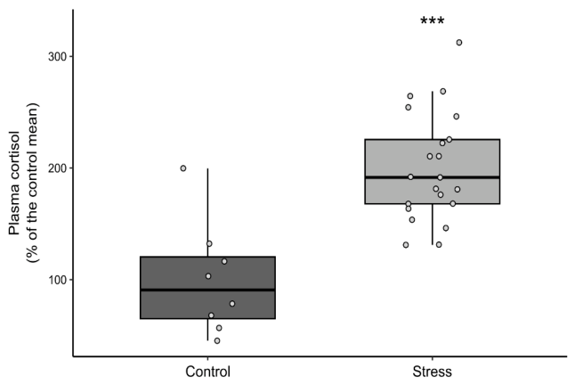
Features are presented as mean ± SEM unless otherwise stated. Plasma cortisol was measured in reference (n = 8) and stressed (n = 21) fish; the detailed assay procedure is reported in Laique et al. (2026). Cortisol was expressed as a percentage of the reference-group mean and was higher in stressed fish (Wilcoxon rank-sum test: W = 14, p < 0.001).
4. Results
4.1. Image Acquisition and Photometric Variation
Photographs were acquired with the camera in program auto-exposure mode. Aperture (f/2.8), sensitivity (ISO 100), white balance (manual) and flash suppression were constant across all 84 images of stressed fish, with a single exception at f/8. Shutter speed and exposure compensation, however, varied both within and between sessions. Sensor exposure (Eq. 7) differed by a mean of +0.008 stops between the pre- and post-stress sessions, indicating no systematic difference in exposure between imaging days, but the per-fish paired difference had a standard deviation of 0.90 stops and ranged from −2.68 to +2.32 stops. Twenty-two of 42 image pairs (52%) differed by more than 0.5 stops and nine (21%) by more than one stop.
This pattern, negligible systematic offset combined with substantial random variation implies that uncorrected exposure differences would inflate the variance of all photometric features without biasing their means. All features reported below were therefore computed after photometric normalization, and all effects are additionally adjusted for residual per-image exposure.
4.2. Statistical Approach and Assumption Checks
For each feature, a repeated-measures two-way ANOVA (day × side) was fitted to the fish-level compilation, followed by regression of the per-fish change on the corresponding change in log₂ sensor exposure. The intercept of that regression is reported as the exposure-adjusted effect.
Residual normality was violated for spot-to-background contrast (Shapiro–Wilk p = 0.002), spot grayscale intensity (p = 0.001) and background grayscale intensity (p = 0.008), and homogeneity of variance was violated for contrast (Levene p = 0.006) and spot intensity (p = 0.016). All primary conclusions were therefore verified with the Wilcoxon signed-rank test and with bias-corrected bootstrap confidence intervals (10,000 resamples); in every case the non-parametric and bootstrap results agreed closely with the parametric estimates, and are reported alongside them. Because the design has two levels of each factor, sphericity is satisfied by construction and no correction was applied.
Spot-to-background contrast was designated the primary outcome. Spot intensity, background intensity and spot area are secondary outcomes, with p-values adjusted across the three by the Benjamini–Hochberg procedure.
4.3. Spot-to-Background Contrast
Spot-to-background contrast, computed in linear light for each operculum and then averaged, increased from −0.9051 ± 0.0074 before confinement to −0.8568 ± 0.0120 afterwards (mean ± SEM, n = 21 fish, 42 opercula). Because contrast is negative for dark spots on lighter skin, this represents a reduction in the magnitude of contrast: spots became less distinct from the surrounding opercular tissue.
The repeated-measures ANOVA showed a significant main effect of day, F (1,20) = 26.32, p < 0.001 partial η² = 0.568. Neither the main effect of side, F (1,20) = 0.41, p = 0.527, partial η² = 0.020, nor the day × side interaction, F (1,20) = 1.28, p = 0.271, was significant, indicating that the change was comparable on both opercula.
After adjustment for per-image exposure, the estimated change was +0.0483 (95% CI [0.0328,0.0639], p < 0.001), essentially identical to the unadjusted paired change of +0.0482 and corresponding to a large within-subject effect (d_z= 0.95). The exposure covariate was not itself a significant predictor of the change in contrast (slope = -0.013 per stop,r = -0.24, p = 0.126). Non-parametric and bootstrap analyses confirmed the result (Wilcoxon signed-rank W = 55, p<0.001 bootstrap 95% CI [0.0333,0.0638]).
4.4. Spot Grayscale Intensity
Mean spot luminance increased from 0.0267 ± 0.0033 to 0.0609 ± 0.0075 in linear light (0.1624 ± 0.0111 to 0.2489 ± 0.0167 on the sRGB-encoded scale; mean ± SEM, n = 42 opercula), indicating that the spots themselves became lighter.
The main effect of day was significant, F (1, 20) = 26.90, p < 0.001, partial η² = 0.574. There was no effect of side, F (1, 20) = 0.01, p = 0.938, and no day × side interaction, F(1, 20) = 0.00, p = 0.945. The exposure-adjusted change was +0.0343 (95% CI [0.0216, 0.0470], p < 0.001; Benjamini–Hochberg-adjusted p < 0.001), against an unadjusted change of +0.0342, with d_z = 0.84. The exposure covariate showed a weak negative association that did not reach significance (slope = −0.0068 per stop, r = −0.15, p = 0.338). The effect was confirmed non-parametrically (Wilcoxon signed-rank W = 41, p < 0.001) and by bootstrap (95% CI [0.0231, 0.0473]).
4.5. Background Grayscale Intensity
Mean luminance of the local background annulus surrounding each spot increased from 0.2589 ± 0.0167 to 0.3825 ± 0.0250 in linear light (0.5337 ± 0.0158 to 0.6388 ± 0.0178 sRGB-encoded scale).
The main effect of day was significant, F(1, 20) = 41.44, p < 0.001, partial η² = 0.674, with no effect of side, F(1, 20) = 0.38, p = 0.544, and no interaction, F(1, 20) = 0.95, p = 0.341. The exposure-adjusted change was +0.1239 (95% CI [0.0733, 0.1745], p < 0.001; Benjamini–Hochberg-adjusted p < 0.001), against an unadjusted change of +0.1235, with d_z = 0.75. The effect was confirmed non-parametrically (Wilcoxon signed-rank W = 72, p < 0.001) and by bootstrap (95% CI [0.0772, 0.1757]). The exposure covariate showed a weak negative association that did not reach significance (slope = −0.0454 per stop, r = −0.25, p = 0.113).
The background lightened by a greater absolute amount than the spots themselves (+0.124 versus +0.034 in linear luminance; +0.105 versus +0.087 on the encoded scale), while the proportional increase was greater for the spots (2.82 ± 0.42 versus 1.63 ± 0.12 fold; per-operculum means ± SEM, n = 42). Because spot-to-background contrast is a ratio, it is the proportional change that determines it; this comparison is examined in Section 5.2.
4.6. Spot Area
Mean segmented spot area decreased from 26,978 ± 1,740 px to 24,950 ± 1,719 px, a reduction of 7.5%. The main effect of day was significant, F (1,20) = 45.28, p < 0.001, partial η² = 0.694, with no effect of side, F (1,20) = 0.09, p = 0.771, and no interaction, F (1,20) = 0.02, p = 0.891. The exposure-adjusted change was -2,027 px (95% CI [-2,625, -1,429], p < 0.001; BH-adjusted p<0.001), equivalent to -7.5% (95% CI [-9.7%, -5.3%]), with d_z= -1.07 (W = 43, p<0.001; bootstrap 95% CI [-2,602, -1,473]). Of the four features, spot area showed the weakest association with exposure (r = -0.06, p = 0.717), as expected for a geometric rather than photometric quantity. Spot area is derived from the segmentation mask, and a spot with reduced contrast against its background may yield a smaller mask independently of any change in the underlying pigmented region. This result should therefore be interpreted alongside, rather than as independent confirmation of, the photometric findings; the limitation is addressed in section 5.6.
4.7. Comparison with the Reference Group
Reference fish (n = 8) were photographed at a single timepoint on the first experimental day, so a group × time interaction was not estimable and comparisons are necessarily cross-sectional. Because the reference session differed from the stressed sessions in both illumination and working distance, comparisons were restricted to spot-to-background contrast, which is invariant to multiplicative changes in illumination and to image scale.
Mean contrast in reference fish was -0.9210 ± 0.0113. This did not differ from stressed fish measured before confinement (-0.9051 ± 0.0085; mean difference -0.0160, 95% CI [-0.0461,0.0141], Welch t(15.4) = -1.13,p = 0.276,d = -0.43) but differed markedly from the same fish after confinement (-0.8568 ± 0.0151; mean difference -0.0642, 95% CI [-0.1029,-0.0255],Welch t(25.6) = -3.41, p = 0.002, d = -1.04).
Reference group therefore resembled pre-stress fish and were clearly separated from post-stress fish on a scale-invariant measure of spot distinctness (Figure 12). Because the reference group was imaged only once, this comparison cannot exclude elapsed time, tank habituation or repeated handling as contributors to the change observed in the stressed group; this is addressed in the discussion section.
4.8. Plasma Cortisol
As previously reported in Laique et al. [31], plasma cortisol, expressed as a percentage of the reference-group mean, was higher in confined fish (n = 21) than in reference fish (n = 8) (Wilcoxon rank-sum test,W = 14,p < 0.001), confirming that the confinement protocol elicited a physiological stress response. Assay details are reported in Laique et al. [31].
Figure 13.
Plasma cortisol (% of control mean) in control (n = 8) and stress-treated fish (n = 21). Boxplots show medians and IQR; points represent individual fish. Cortisol levels were higher in the stress group (Wilcoxon rank-sum test, W = 14, p < 0.001; *** p < 0.001) - Data previously published in Laique et al. (2026), reproduced under CC-BY.
Figure 13.
Plasma cortisol (% of control mean) in control (n = 8) and stress-treated fish (n = 21). Boxplots show medians and IQR; points represent individual fish. Cortisol levels were higher in the stress group (Wilcoxon rank-sum test, W = 14, p < 0.001; *** p < 0.001) - Data previously published in Laique et al. (2026), reproduced under CC-BY.
5. Discussion
5.1. Summary of Findings
The aim of this study was to establish whether fading of melanin-based opercular spots in Atlantic salmon can be quantified reliably enough to support its evaluation as a stress indicator, and specifically whether such fading can be distinguished from the image-acquisition variation that confounds longitudinal photometry in live animals. Following 18 h of confinement, spots became lighter (∆ = 0.087,95% CI [0.061,0.112]), the surrounding opercular tissue also lightened (Δ = 0.105,95% CI [0.069,0.141]), spot-to-background contrast fell in magnitude (Δ = 0.048,95% CI [0.033,0.064]), and segmented spot area decreased by 7.5% (95% CI [5.3,9.7]). Effects were large (d_z = 0.88-1.07), consistent across both opercula, and unchanged after adjustment for per-image sensor exposure.
The photometric control is central to interpreting these results. Sensor exposure varied by up to 2.7 stops between paired photographs of the same individual, with a within-session standard deviation of approximately 0.8 stops. Critically, this variation was random rather than systematic: mean exposure differed between sessions by only 0.008 stops. Uncorrected, it would therefore have inflated the variance of every photometric feature without biasing their means, which is what the exposure-adjusted estimates confirm, being numerically almost identical to the unadjusted ones while resting on a defensible basis. This distinction matters, because a systematic exposure offset of the magnitude observed here between individual pairs would have been sufficient to generate the entire reported effect.
5.2. Spots Faded More Than the Surrounding Skin
Both spots and surrounding tissue lightened, which raises the question of whether the observed change reflects spot-specific fading or a generalized paling of the operculum. Expressed in linear reflectance, spot luminance increased by a factor of 2.82 ± 0.42 while background luminance increased by 1.63 ± 0.12 (per-operculum means ± SEM). The proportional increase was significantly greater for spots than for the surrounding tissue (paired t-test on log fold-change, t(41)= 6.41, p<0.001).
This is the result that distinguishes the two interpretations. Generalized paling of the operculum would produce a common multiplicative change in both regions and would leave normalized contrast unaltered, since Weber contrast is invariant to multiplicative scaling. The observed reduction in contrast magnitude therefore requires that the two regions changed by different proportions, and the direction of that difference indicates that the pigmented spots lightened more than the tissue around them. Melanin-bearing regions responded more strongly to confinement than adjacent non-spotted skin.
The comparison must be made in linear light. Weber contrast is invariant to multiplicative scaling of the signal only when the signal is proportional to scene radiance; on gamma-encoded values an illumination change alters the recorded contrast, and the fold-changes are compressed (1.53 for spots and 1.20 for the background, against 2.82 and 1.63 in linear reflectance). Linearization therefore determines both the magnitude of the effect and the validity of the invariance argument on which the interpretation rests, although the ordering of the two proportional changes is preserved on the encoded scale.
5.3. Mechanistic Interpretation
Two endocrine pathways predict stress-associated fading of melanin-based pigmentation, and they differ in the timescale and the morphological signature they produce. MCH-mediated melanosome aggregation operates within seconds to minutes, is readily reversible, and produces a change in apparent intensity through translocation of pigment organelles within existing melanophores; spot boundaries should be largely preserved [45]. Cortisol-driven upregulation of ASP antagonizes α−MSH and suppresses melanosome dispersion over hours to days, and sustained suppression would be expected to affect the spot margin, where melanophore density is lowest, before the spot centre [62].
Our observations are consistent with a contribution from both. The magnitude of the intensity change over 18 h, together with the reduction in spot area, is more readily explained by a process acting on the spot as a whole, including its periphery, than by rapid melanosome translocation alone. We interpret the area reduction as consistent with fading progressing inward from the spot margin, but with an important caveat addressed in Section 5.6: spot area is derived from a segmentation mask, and a spot of reduced contrast may yield a smaller mask irrespective of any change in the underlying pigmented region. Discriminating these pathways would require sampling at multiple timepoints within the first hours after the stressor and following recovery, which the present design cannot support.
5.4. Relationship to Previous Work
Previous research on melanin-based pigmentation in salmonids has reported that individuals with more spots show reduced cortisol responsiveness and differ in behavioral stress coping [26,29,30], and Thorsen [63] reported that opercular spots fade in response to crowding and netting. These studies relied on manual identification of spots and qualitative or semi-quantitative assessment of change. Our previous study [31] automated spot detection, registration and segmentation, and demonstrated as proof of principle that spot grayscale intensity shifts following confinement. The present study extends that work by establishing that the shift survives photometric control, by quantifying it with effect sizes and confidence intervals, and by showing that it is spot-specific rather than a generalized change in skin luminance.
A tension in this literature deserves comment. Stress in salmonids is frequently associated with skin darkening rather than paling: subordinate Arctic charr darken during social interaction, mediated by α−MSH and other POMC-derived peptides [22], and prolonged stress and dark-background adaptation both elevate circulating α−MSH, which disperses melanosomes and darkens the skin. Our result runs in the opposite direction. We suggest this reflects a genuine distinction rather than a contradiction. Chronic social subordination and background matching act on dermal melanophore populations across the body surface over days, whereas acute confinement engages MCH- and cortisol-mediated pathways that aggregate pigment and suppress dispersion over hours. The discrete opercular spots may also be regulated differently from diffuse dermal pigmentation. Resolving this would require simultaneous measurement of α−MSH, MCH and cortisol alongside imaging, which we identify as a priority for subsequent work.
The direction of our finding also bears on one of the principal confounds in this experiment. The fish were held in dark green tanks, and background adaptation to a dark substrate predicts skin darkening. The observed lightening is therefore opposite to what background adaptation would produce, which argues against it as an explanation for the present result, though it does not exclude it as a source of variance.
5.5. Methodological Contribution
Quantitative measurement of animal coloration from digital photographs is an established methodology, and the acquisition problems encountered here have been described in that literature for nearly two decades. Stevens et al. [59] noted that studies using digital photography are frequently unaware of the non-linearity of camera response to light intensity and set out procedures for linearizing camera response and calibrating against reflectance standards. Akkaynak et al. [3] and Troscianko and Stevens [64] formalized these procedures, the latter in a freely available toolbox. Both approaches, however, require raw sensor data and a physical reflectance standard within the frame of every photograph.
Neither precondition is typically met in aquaculture research or production, where imaging is performed on wet, mobile animals under time pressure, and neither can be satisfied retrospectively for an existing image archive. The procedure introduced here substitutes an analytically recoverable radiometric reference for a physical one: the exposure metadata written to every consumer image file determines the sensor exposure exactly and dividing linearized pixel values by this quantity places images acquired under automatic exposure on a common relative scale. We regard this as complementary to calibrated photography rather than a substitute for it. The procedure recovers relative exposure, not absolute reflectance, and cannot correct for changes in scene illumination, spectral composition, or camera-specific tone curves departing from the sRGB standard. It is, however, applicable to data already collected, which conventional calibration is not.
Segmentation quality bounds the validity of every photometric feature reported here, since spot intensity, background intensity and area are all computed from the predicted mask. The fine-tuned SAM 2.1 model achieved a Dice of 0.89 ± 0.06 against manual annotations, compared with 0.80 ± 0.17 for global Otsu thresholding and 0.78 ± 0.20 for local adaptive thresholding (Table 6). Because both baselines were given the same bounding-box prior as the model prompt, the margin is attributable to segmentation rather than localization. The difference in variability is more consequential than the difference in means: the standard deviation of the learned segmenter is roughly a third that of either baseline, and 10% of spots fell below a Dice of 0.5 under adaptive thresholding compared with none under SAM 2.1. For a measurement instrument, this consistency matters more than mean accuracy, since sporadic segmentation failures introduce feature errors that are neither detectable nor correctable downstream. The margin was largest where spot margins were diffuse, the condition that becomes more common after confinement, as spot contrast declines, so classical thresholding is least reliable in precisely the regime where the measurement matters most. A companion manuscript on the same dataset [32] characterizes spot architecture and its repeatability using a skin-referenced intensity descriptor with an in-frame exposure proxy. The present study differs in that the acquisition correction is derived from the recorded camera settings and is applied to the image before measurement, and in that spot area and local background are analysed alongside contrast; the two approaches are complementary tests of whether the same change survives different acquisition controls.
5.6. Limitations
- Reference group design: Reference group were photographed at a single timepoint on the first experimental day. A group × time interaction is therefore not estimable, and the comparison in Section 4.7 is cross-sectional. Reference fish did not differ from pre-stress fish but differed markedly from post-stress fish in spot-to-background contrast, which is consistent with an effect of confinement; however, elapsed time in the tank, habituation, circadian variation in pigmentation, and the handling required for the first photographic session all remain unexcluded as contributors. This is the principal limitation of the study, and it constrains the design rather than the analysis: no reanalysis of the present data can address it.
- Spot area is not independent evidence: A spot with reduced contrast against its background may yield a smaller segmentation mask under any threshold-dependent method. The area result should therefore be read as consistent with, rather than as independent confirmation of, the photometric findings.
- Acquisition conditions: Images were captured in a booth open at the front, so ambient daylight contributed variably to the interior illumination, and the camera operated in automatic exposure mode. Our normalization addresses the resulting exposure variation but cannot recover information absent from the recorded data; in particular, underexposed frames carry lower signal-to-noise ratios that scaling amplifies along with the signal. Raw capture with an in-frame calibration target would remove this limitation entirely.
- Statistical assumptions: Residual normality was violated for three of four features and homogeneity of variance for two. All primary conclusions were verified by non-parametric and bootstrap methods, which agreed closely with the parametric estimates, but the parametric p-values should be read with this in mind.
- Generalizability: The study involved a single stock at a single facility, one stressor, one post-stress timepoint, and 29 animals in total. Whether the effect generalizes across stocks, pigmentation phenotypes, stressor types and production environments is untested.
- Anaesthesia and handling: All images were acquired from netted, anaesthetised fish, and the post-confinement and reference images were taken following a lethal dose of MS-222. Deep anaesthesia may alter sympathetic control of chromatophores and can therefore affect apparent pigmentation, so anaesthetic state is partly confounded with imaging session. That the reference fish were terminally anaesthetised in the same way, yet did not differ from pre-confinement fish in spot-to-background contrast, argues against anaesthesia alone accounting for the result, but the design remains confounded in this respect.
- Physiological linkage: Plasma cortisol confirmed at the group level that the confinement protocol elicited a stress response, but individual cortisol concentrations were not related to individual fading. Establishing that association is the necessary next step toward biomarker status.
5.7. Implications and Future Directions
Operational welfare indicators currently used in salmon production comprise a mixture of handling-based and invasive measures. Morphological indicators such as fin condition, skin condition, vertebral deformity and sea lice burden require capture and close manual inspection [46,60]. Physiological indicators such as plasma cortisol require blood sampling, and their interpretation is sensitive to sampling latency because the handling required to obtain the sample itself elicits a cortisol response [15,57]. Both classes register a welfare problem principally after it has developed, which limits their utility for preventive management.
An image-based measure of pigmentation offers a different profile: it does not in principle require contact with the animal and could in principle be acquired repeatedly, although the present images were obtained from netted and anaesthetised fish, and reflects a physiological rather than a pathological state. The present study does not establish opercular spot fading as a validated biomarker. Fading in this cohort has been associated with regional brain serotonergic activity [20], indicating that the measured change co-varies with a central stress marker, but whether the relationship is consistent enough at the level of the individual animal to support use as a biomarker remains to be established. What the present study establishes is that the change is measurable, that it is large relative to measurement error once acquisition is controlled, that it is spot-specific rather than a generalized change in skin luminance, and that unhandled fish resemble pre-stress rather than post-stress fish on a scale-invariant measure.
Four priorities follow. First, a longitudinal control group imaged at the same interval without confinement, which would supply the interaction term the present design cannot. Second, correlation of individual cortisol with individual fading, which would connect the optical measurement to the physiological axis it is proposed to index. Third, a time-course and recovery design, which would discriminate the MCH and ASP pathways and establish whether the measure indexes a reversible state or accumulated change. Fourth, acquisition under standardized conditions with raw capture, fixed camera settings, controlled illumination, fixed working distance, and an in-frame calibration target, which would remove the photometric uncertainty that this study has had to address analytically.
Beyond these, testing across multiple stocks, environments and pigmentation phenotypes will be required to assess generalizability and robustness.
6. Conclusions
This study provides a photometrically controlled framework for quantifying the appearance of individual melanin-based opercular spots in Atlantic salmon. Following 18 h of confinement, spots lightened, spot-to-background contrast declined, and spot area decreased, with large effect sizes that were robust to adjustment for image acquisition. Spots lightened proportionally more than adjacent skin, indicating a response localized to pigmented regions rather than a generalized change in opercular luminance. Because the reference group was imaged at a single timepoint, the effect cannot be attributed to confinement to the exclusion of elapsed time, and physiological validation remains outstanding. The framework nonetheless establishes that stress-associated pigmentation change in salmonids can be measured quantitatively from consumer photography, and provides a methodological foundation for the further work required to determine whether it constitutes a useful non-invasive welfare indicator.
Funding
The study is funded by Research Council of Norway—NFR VISSIGN (NMBU Category 3 scholarship is NMBU co-funding as pr contract with NFR- Project number: 324571).
Institutional Review Board Statement
The experiment was conducted in accordance with current local legislation governing the use of live animals in research and was approved by the Norwegian Food Safety Authority under FOTS application ID30246, approval date: 18 April 2023.
Data Availability Statement
The data and scripts that support the findings of this study are openly available in Zenodo at DOI: https://doi.org/10.5281/zenodo.23056749, and the tool for feature generation is available on GitHub at https://github.com/laiquet/multimodal-labeling-tool.git.
Acknowledgments
The authors would like to thank the Institute of Marine Research (IMR), Bergen, Norway, for providing the dataset that made this study possible and SINTEF Ocean, applied research, technology and innovation, for their supervisory interest in the Project. OpenAI (GPT 5.5) and Anthropic (Opus 5.5) were utilized during the preparation of this manuscript to assist with paraphrasing, grammar correction and improving overall readability. The content was reviewed and edited as necessary to ensure accuracy and alignment with the final published article.
Conflicts of Interest
The authors declare that the research was conducted in the absence of any commercial or financial relationships that could be construed as a potential conflict of interest.
References
- Adams, C. E.; Turnbull, J. F.; Bell, A.; Bron, J. E.; Huntingford, F. A. Multiple determinants of welfare in farmed fish: Stocking density, disturbance, and aggression in Atlantic salmon (Salmo salar). Can. J. Fish. Aquat. Sci. 2007, 64(2), 336–344. [Google Scholar] [CrossRef]
- Ahmed, M. S.; Aurpa, T. T.; Azad, M. A. K. Fish disease detection using imagebased machine learning technique in aquaculture. J. King Saud University–Computer Inf. Sci. 2022, 34(8), 5170–5182. [Google Scholar] [CrossRef]
- Akkaynak, D.; Treibitz, T.; Xiao, B.; Gürkan, U. A.; Allen, J. J.; Demirci, U.; Hanlon, R. T. Use of commercial off-the-shelf digital cameras for scientific data acquisition and scene-specific color calibration. J. Opt. Soc. Am. A 2014, 31(2), 312–321. [Google Scholar] [CrossRef]
- Banno, K.; Kaland, H.; Crescitelli, A. M.; Tuene, S. A.; Aas, G. H.; Gansel, L. C. A novel approach for wild fish monitoring at aquaculture sites: Wild fish presence analysis using computer vision. Aquac. Environ. Interact. 2022, 14, 97–112. [Google Scholar] [CrossRef]
- Bekkozhayeva, D.; Cisar, P. Image-based automatic individual identification of fish without obvious patterns on the body (scale pattern). Appl. Sci. 2022, 12(11), 5401. [Google Scholar] [CrossRef]
- Bradski, G. The OpenCV library. Dr. Dobb's J. Softw. Tools 2000, 25(11), 120–125. [Google Scholar] [CrossRef]
- Burke, M.; Nikolic, D.; Fabry, P.; Rishi, H.; Telfer, T. C.; Rey-Planellas, S. Precision farming in aquaculture: Use of a non-invasive, AI-powered real-time automated behavioural monitoring approach to predict gill health and improve welfare in Atlantic salmon (Salmo salar) aquaculture farms [Preprint]. SSRN 2024. [Google Scholar] [CrossRef]
- Buslaev, A.; Iglovikov, V. I.; Khvedchenya, E.; Parinov, A.; Druzhinin, M.; Kalinin, A. A. Albumentations: Fast and flexible image augmentations. Information 2020, 11(2), 125. [Google Scholar] [CrossRef]
- Cerdá-Reverter, J. M.; Agulleiro, M. J.; Guillot, R.; Sánchez, E.; Ceinos, R.; Rotllant, J. Fish melanocortin system. Eur. J. Pharmacol. 2011, 660(1), 53–60. [Google Scholar] [CrossRef]
- Cerdá-Reverter, J. M.; Haitina, T.; Schiöth, H. B.; Peter, R. E. Gene structure of the goldfish agouti-signaling protein: A putative role in the dorsal–ventral pigment pattern of fish. Endocrinology 2005, 146(3), 1597–1610. [Google Scholar] [CrossRef]
- Cesarini, J. P. Melanins and their possible roles through biological evolution. Adv. Space Res. 1996, 18(12), 35–40. [Google Scholar] [CrossRef]
- Cisar, P.; Bekkozhayeva, D.; Movchan, O.; Saberioon, M.; Schraml, R. Computer vision based individual fish identification using skin dot pattern. Sci. Rep. 2021, 11(1), 16904. [Google Scholar] [CrossRef]
- Dubrofsky, E. Homography estimation. In Diplomová práce; Univerzita Britské Kolumbie: Vancouver, 2009; p. 5. [Google Scholar]
- Dwyer, B.; Nelson, J.; Hansen, T.; Solawetz, J. Roboflow (Version 1.0) [Computer software]. 2025. Available online: https://roboflow.com.
- Ellis, T.; Yildiz, H. Y.; López-Olmeda, J.; Spedicato, M. T.; Tort, L.; Øverli, Ø.; Martins, C. I. M. Cortisol and finfish welfare. Fish. Physiol. Biochem. 2012, 38(1), 163–188. [Google Scholar] [CrossRef]
- Fischler, M. A.; Bolles, R. C. Random sample consensus: A paradigm for model fitting with applications to image analysis and automated cartography. Commun. ACM 1981, 24(6), 381–395. [Google Scholar] [CrossRef]
- Gröneveld, D.; Balm, P. H. M.; Wendelaar Bonga, S. E. Biphasic effect of MCH on α-MSH release from the tilapia (Oreochromis mossambicus) pituitary. Peptides 1995, 16(5), 945–949. [Google Scholar] [CrossRef]
- Gupta, A.; Bringsdal, E.; Knausgård, K. M.; Goodwin, M. Accurate wound and lice detection in Atlantic salmon fish using a convolutional neural network. Fishes 2022, 7(6), 345. [Google Scholar] [CrossRef]
- Gunnes, M.; Green, E. A. L.; Andersen, I. L.; Øverli, Ø. Condition-associated modulation of melanin-based skin pigmentation in juvenile Atlantic salmon (Salmo salar) (under review). 2026a. [Google Scholar]
- Gunnes, M.; Laique, T.; Gundersen, H. N.; Folkedal, O.; Nilsson, J.; Øverli, Ø.; Sørensen, C. Stress-induced fading of melanin-based skin pigmentation is associated with brain serotonergic activity in Atlantic salmon. under review. 2026b. [Google Scholar]
- Hoekstra, H. E. Genetics, development and evolution of adaptive pigmentation in vertebrates. Heredity 2006, 97(3), 222–234. [Google Scholar] [CrossRef]
- Höglund, E.; Balm, P. H. M.; Winberg, S. Skin darkening, a potential social signal in subordinate Arctic charr (Salvelinus alpinus): The regulatory role of brain monoamines and pro-opiomelanocortin-derived peptides. J. Exp. Biol. 2000, 203(11), 1711–1721. [Google Scholar] [CrossRef]
- Jocher, G.; Chaurasia, A.; Qiu, J. Ultralytics YOLOv8 (Version 8.0.0) [Computer software]. 2023. Available online: https://github.com/ultralytics/ultralytics.
- Kawauchi, H. Functions of melanin-concentrating hormone in fish. J. Exp. Zool. Part A Comp. Exp. Biol. 2006, 305(9), 751–760. [Google Scholar] [CrossRef]
- Keihani, R.; Gomes, A. S.; Balseiro, P.; Handeland, S. O.; Gorissen, M.; Arukwe, A. Evaluation of stress in farmed Atlantic salmon (Salmo salar) using different biological matrices. Comp. Biochem. Physiol. Part A Mol. Integr. Physiol. 2024, 298, 111743. [Google Scholar] [CrossRef]
- Khan, U. W.; Øverli, Ø.; Hinkle, P. M.; Pasha, F. A.; Johansen, I. B.; Berget, I.; Silva, P. I. M.; Kittilsen, S.; Höglund, E.; Omholt, S. W.; Våge, D. I. A novel role for pigment genes in the stress response in rainbow trout (Oncorhynchus mykiss). Sci. Rep. 2016, 6(1), 28969. [Google Scholar] [CrossRef]
- Kim, S. J.; Lin, H. T.; Lu, Z.; Süsstrunk, S.; Lin, S.; Brown, M. S. A new in-camera imaging model for color computer vision and its application. IEEE Trans. Pattern Anal. Mach. Intell. 2012, 34(12), 2289–2302. [Google Scholar] [CrossRef]
- Kingma, D. P.; Ba, J. Adam: A method for stochastic optimization. arXiv 2014. [Google Scholar] [CrossRef]
- Kittilsen, S.; Johansen, I. B.; Braastad, B. O.; Øverli, Ø. Pigments, parasites and personality: Towards a unifying role for steroid hormones? PLoS ONE 2012, 7(4), e34281. [Google Scholar] [CrossRef]
- Kittilsen, S.; Schjolden, J.; Beitnes-Johansen, I.; Shaw, J. C.; Pottinger, T. G.; Sørensen, C.; Braastad, B. O.; Bakken, M.; Øverli, Ø. Melanin-based skin spots reflect stress responsiveness in salmonid fish. Horm. Behav. 2009, 56(3), 292–298. [Google Scholar] [CrossRef]
- Laique, T.; Gunnes, M.; Folkedal, O.; Nilsson, J.; Green, E. A. L.; Gundersen, H. N.; Øverli, Ø.; Ullah, H. Quantification of opercular pigmentation changes in farmed Atlantic salmon: A novel application for computer vision in fish welfare assessment. Fishes 2026, 11(5), 271. [Google Scholar] [CrossRef]
- Laique, T.; Gunnes, M.; Øverli, Ø.; Ullah, H.; Ocepek, M. Computer vision-based phenotyping of melanin-based opercular spot architecture in farmed Atlantic salmon: toward image-derived welfare monitoring. J. Anim. Sci. (under review) 2026. [Google Scholar]
- Land, E. H.; McCann, J. J. Lightness and retinex theory. J. Opt. Soc. Am. 1971, 61(1), 1–11. [Google Scholar] [CrossRef]
- Leclercq, E.; Taylor, J. F.; Migaud, H. Morphological skin colour changes in teleosts. Fish. Fish. 2010, 11(2), 159–193. [Google Scholar] [CrossRef]
- Lin, T.-Y.; Maire, M.; Belongie, S.; Hays, J.; Perona, P.; Ramanan, D.; Dollár, P.; Zitnick, C. L. Microsoft COCO: Common objects in context. In Computer Vision – ECCV 2014; Fleet, D., Pajdla, T., Schiele, B., Tuytelaars, T., Eds.; Springer, 2014; pp. 740–755. [Google Scholar] [CrossRef]
- Lowe, D. G. Distinctive image features from scale-invariant keypoints. Int. J. Comput. Vis. 2004, 60(2), 91–110. [Google Scholar] [CrossRef]
- Lu, D.; Willard, D.; Patel, I. R.; Kadwell, S.; Overton, L.; Kost, T.; Luther, M.; Chen, W.; Woychik, R. P.; Wilkison, W. O.; Cone, R. D. Agouti protein is an antagonist of the melanocyte-stimulating-hormone receptor. Nature 1994, 371(6500), 799–802. [Google Scholar] [CrossRef]
- Ludwig, D. S.; Mountjoy, K. G.; Tatro, J. B.; Gillette, J. A.; Frederich, R. C.; Flier, J. S.; Maratos-Flier, E. Melanin-concentrating hormone: A functional melanocortin antagonist in the hypothalamus. Am. J. Physiol. – Endocrinol. Metab. 1998, 274(4), E627–E633. [Google Scholar] [CrossRef]
- Larsen, S. Objective analysis of melanin spots as welfare signals in Atlantic salmon using AI-based computer vision. Master's thesis, Norwegian University of Science and Technology, NTNU Open, 2024. Available online: https://hdl.handle.net/11250/3154352.
- Mackintosh, J. A. The antimicrobial properties of melanocytes, melanosomes and melanin and the evolution of black skin. J. Theor. Biol. 2001, 211(2), 101–113. [Google Scholar] [CrossRef]
- Mathiassen, J. R.; Misimi, E.; Skavhaug, A. A simple computer vision method for automatic detection of melanin spots in Atlantic salmon fillets. In International Machine Vision and Image Processing Conference (IMVIP 2007); IEEE, 2007; pp. 192–200. [Google Scholar] [CrossRef]
- 2025. Norwegian fish health report 2024 (Report No. 1b/2025). Norwegian Veterinary Institute. Available online: https://www.vetinst.no/rapporter-og-publikasjoner/rapporter/2025/norwegian-.
- Muja, M.; Lowe, D. G. Fast approximate nearest neighbors with automatic algorithm configuration. Proc. Fourth Int. Conf. Comput. Vis. Theory Appl. 2009, Vol. 1, 331–340. [Google Scholar] [CrossRef]
- Ziaei, M. M.; Urban, J.; Cisar, P. Image-Based Individual Fish Identification as a Substitute for Invasive Methods: State-of-the-Art and Research Gaps. Rev. Aquac. 2025, 17(4), e70078. [Google Scholar] [CrossRef]
- Nilsson Sköld, H.; Aspengren, S.; Wallin, M. Rapid colour change in fish and amphibians: Function, regulation and emerging applications. Pigment Cell Melanoma Res. 2013, 26(1), 29–38. [Google Scholar] [CrossRef]
- Noble, C.; Gismervik, K.; Iversen, M. H.; Kolarevic, J.; Nilsson, J.; Stien, L. H.; Turnbull, J. F. (Eds.) Welfare indicators for farmed Atlantic salmon: Tools for assessing fish welfare; Nofima, 2018. [Google Scholar]
- Otsu, N. A threshold selection method from gray-level histograms. *IEEE Trans. Syst. Man. Cybern. 1979, 9*(1), 62–66. [Google Scholar] [CrossRef]
- Overton, K.; Dempster, T.; Oppedal, F.; Kristiansen, T. S.; Gismervik, K.; Stien, L. H. Salmon lice treatments and salmon mortality in Norwegian aquaculture: A review. Rev. Aquac. 2019, 11(4), 1398–1417. [Google Scholar] [CrossRef]
- Ramanath, R.; Drew, M. S. White balance. In Computer Vision: A Reference Guide; Springer International Publishing: Cham, 2021; pp. 1387–1391. [Google Scholar] [CrossRef]
- Ranjan, R.; Tsukuda, S.; Good, C. MortCam: An artificial intelligence-aided fish detection and alert system for recirculating aquaculture. Aquac. Eng. 2023, 102, 102341. [Google Scholar] [CrossRef]
- Ravi, N.; Gabeur, V.; Hu, Y.-T.; Hu, R.; Ryali, C.; Ma, T.; Khedr, H.; Rädle, R.; Rolland, C.; Gustafson, L.; Mintun, E.; Pan, J.; Alwala, K. V.; Carion, N.; Wu, C.-Y.; Girshick, R.; Dollár, P.; Feichtenhofer, C. SAM 2: Segment anything in images and videos. arXiv 2024. [Google Scholar] [CrossRef]
- Rey, S.; Little, D.; Ellis, M. Farmed fish welfare practices: Salmon farming as a case study; Global Aquaculture Alliance, 2019; Available online: https://www.globalseafood.org/.
- Riley, P. A. Melanin. Int. J. Biochem. Cell Biol. 1997, 29(11), 1235–1239. [Google Scholar] [CrossRef]
- Roulin, A. The evolution, maintenance and adaptive function of genetic colour polymorphism in birds. Biol. Rev. 2004, 79(4), 815–848. [Google Scholar] [CrossRef]
- Ryali, C.; Hu, Y.-T.; Bolya, D.; Wei, C.; Fan, H.; Huang, P.-Y.; Aggarwal, V.; Chowdhury, A.; Poursaeed, O.; Hoffman, J.; Malik, J.; Li, Y.; Feichtenhofer, C. Hiera: A hierarchical vision transformer without the bells-and-whistles. Proc. 40th Int. Conf. Mach. Learn. (PMLR 2023, Vol. 202, 29441–29454. [Google Scholar]
- Saberioon, M.; Gholizadeh, A.; Cisar, P.; Pautsina, A.; Urban, J. Application of machine vision systems in aquaculture with emphasis on fish: State-of-the-art and key issues. Rev. Aquac. 2017, 9(4), 369–387. [Google Scholar] [CrossRef]
- Sadoul, B.; Geffroy, B. Measuring cortisol, the major stress hormone in fishes. J. Fish. Biol. 2019, 94(4), 540–555. [Google Scholar] [CrossRef]
- Shimomura, Y.; Mori, M.; Sugo, T.; Ishibashi, Y.; Abe, M.; Kurokawa, T.; Onda, H.; Nishimura, O.; Sumino, Y.; Fujino, M. Isolation and identification of melanin-concentrating hormone as the endogenous ligand of the SLC-1 receptor. Biochem. Biophys. Res. Commun. 1999, 261(3), 622–626. [Google Scholar] [CrossRef]
- Stevens, M.; Párraga, C. A.; Cuthill, I. C.; Partridge, J. C.; Troscianko, T. S. Using digital photography to study animal coloration. Biol. J. Linn. Soc. 2007, 90(2), 211–237. [Google Scholar] [CrossRef]
- Stien, L. H.; Bracke, M. B. M.; Folkedal, O.; Nilsson, J.; Oppedal, F.; Torgersen, T.; Kittilsen, S.; Midtlyng, P. J.; Vindas, M. A.; Øverli, Ø.; Kristiansen, T. S. Salmon Welfare Index Model (SWIM 1.0): A semantic model for overall welfare assessment of caged Atlantic salmon — Review of the selected welfare indicators and model presentation. Rev. Aquac. 2013, 5(1), 33–57. [Google Scholar] [CrossRef]
- Stien, L. H.; Tørud, B.; Gismervik, K.; Lien, M. E.; Medaas, C.; Osmundsen, T.; Kristiansen, T. S.; Størkersen, K. V. Governing the welfare of Norwegian farmed salmon: Three conflict cases. Mar. Policy 2020, 117, 103969. [Google Scholar] [CrossRef]
- Sugimoto, M. Morphological color change in fish: Regulation of pigment cell density and morphology. Microsc. Res. Tech. 2002, 58(6), 496–503. [Google Scholar] [CrossRef]
- Thorsen, D. K. Melanin-based skin pigmentation and stress in Atlantic salmon (Salmo salar). Master's thesis, Norwegian University of Life Sciences, 2019. Available online: https://hdl.handle.net/11250/2605431.
- Troscianko, J.; Stevens, M. Image calibration and analysis toolbox — A free software suite for objectively measuring reflectance, colour and pattern. Methods Ecol. Evol. 2015, 6(11), 1320–1331. [Google Scholar] [CrossRef]
- Willard, D. H.; Bodnar, W.; Harris, C.; Kiefer, L.; Nichols, J. S.; Blanchard, S.; Hoffman, C.; Moyer, M.; Burkhart, W.; Weiel, J.; Luther, M. A.; Wilkison, W. O.; Rocque, W. J. Agouti structure and function: Characterization of a potent α-melanocyte stimulating hormone receptor antagonist. Biochemistry 1995, 34(38), 12341–12346. [Google Scholar] [CrossRef]
- Xu, M.; Yoon, S.; Fuentes, A.; Park, D. S. A comprehensive survey of image augmentation techniques for deep learning. Pattern Recognit. 2023, 137, 109347. [Google Scholar] [CrossRef]
- Yang, X.; Zhang, S.; Liu, J.; Gao, Q.; Dong, S.; Zhou, C. Deep learning for smart fish farming: applications, opportunities and challenges. Rev. Aquac. 2021, 13(1), 66–90. [Google Scholar] [CrossRef]
- Yu, H.; Wang, Z.; Qin, H.; Chen, Y. An automatic detection and counting method for fish lateral line scales of underwater fish based on improved YOLOv5. IEEE Access 2023, 11, 143616–143627. [Google Scholar] [CrossRef]
- Zhang, C.; Zhao, Y.; Yang, W.; Gao, L.; Zhang, W.; Liu, Y.; Sun, C.; Zhou, J.; Wang, H. Computer vision-based deep learning modeling for salmon part segmentation and defect identification. Foods 2025, 14(20), 3529. [Google Scholar] [CrossRef]
- Zhou, Z.; Hitt, N. P.; Letcher, B. H.; Shi, W.; Li, S. Pigmentation-based visual learning for Salvelinus fontinalis individual re-identification. In 2022 IEEE International Conference on Big Data (Big Data); IEEE, 2022; pp. 6850–6852. [Google Scholar] [CrossRef]
Figure 1.
Quantification of fading in melanin-based skin spots under stress in Atlantic salmon (salmo salar) methodology pipeline.
Figure 1.
Quantification of fading in melanin-based skin spots under stress in Atlantic salmon (salmo salar) methodology pipeline.
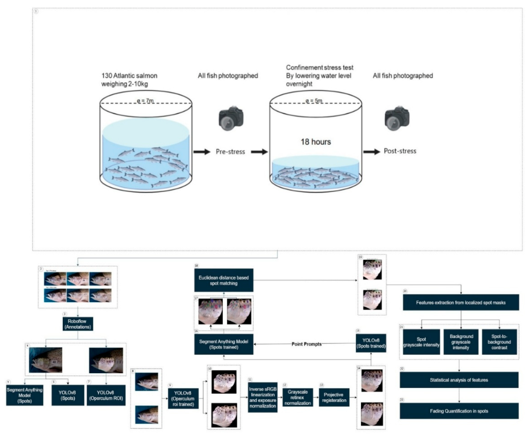
Figure 2.
Close head images of the left and right sides of a salmon specimen on a blue background.
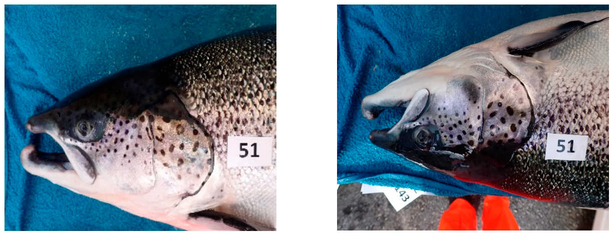
Figure 3.
Spots (left) and operculum (right) region in the close-up image annotated with smart and standard polygon tools in Roboflow.
Figure 3.
Spots (left) and operculum (right) region in the close-up image annotated with smart and standard polygon tools in Roboflow.
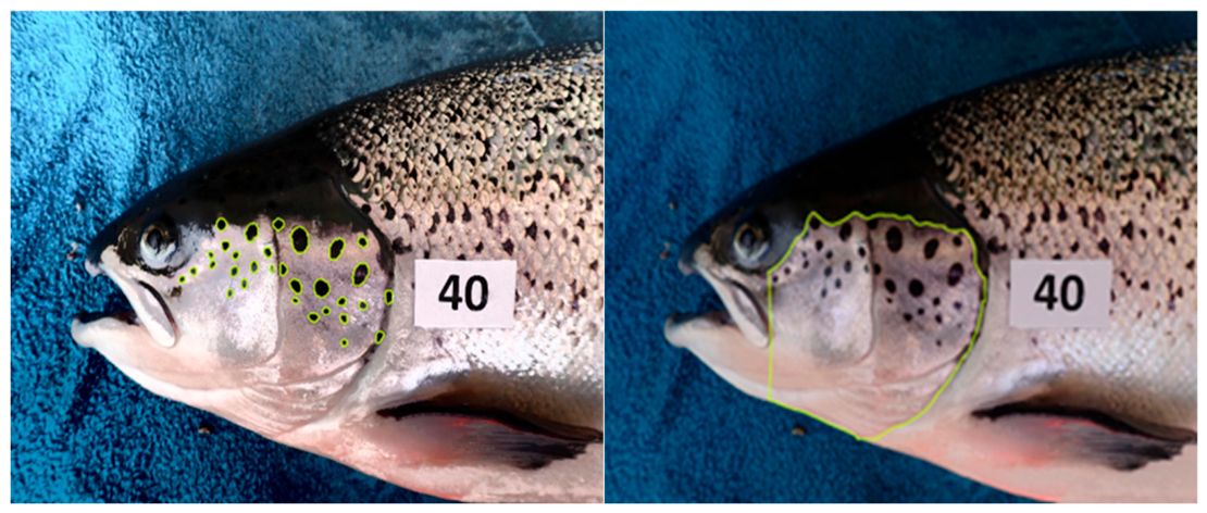
Figure 4.
(a) Bounding box training and validation loss plots, (b) segmentation training and validation loss plots, (c) classification loss, and (d) distributed focal loss training and validation loss plots. Across all loss curves, the model exhibits slight underfitting, specifically the segmentation loss.
Figure 4.
(a) Bounding box training and validation loss plots, (b) segmentation training and validation loss plots, (c) classification loss, and (d) distributed focal loss training and validation loss plots. Across all loss curves, the model exhibits slight underfitting, specifically the segmentation loss.
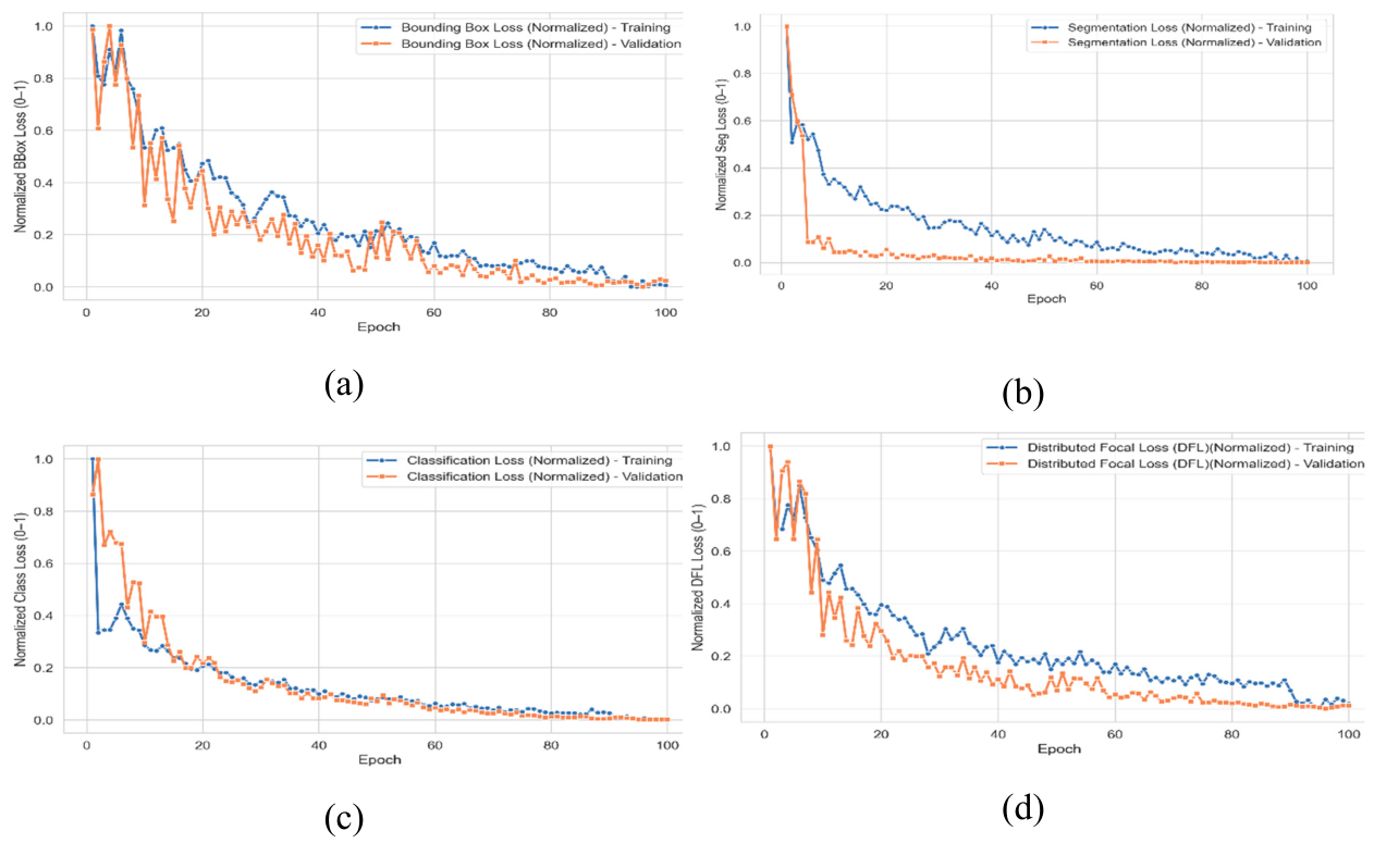
Figure 5.
YOLOv8-spots (a) Bounding box training and validation loss plots, (b) segmentation training and validation loss plots, (c) classification loss, and (d) distributed focal loss training and validation loss plots. Across all loss curves, the model exhibits slight underfitting.
Figure 5.
YOLOv8-spots (a) Bounding box training and validation loss plots, (b) segmentation training and validation loss plots, (c) classification loss, and (d) distributed focal loss training and validation loss plots. Across all loss curves, the model exhibits slight underfitting.
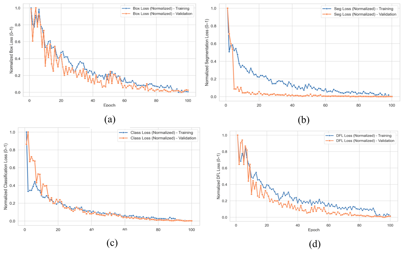
Figure 6.
SAM 2 Training losses (a) Mask loss plot, (b) Intersection-over-Union loss plot, (c) Dice loss plot. All the loss functions are converging.
Figure 6.
SAM 2 Training losses (a) Mask loss plot, (b) Intersection-over-Union loss plot, (c) Dice loss plot. All the loss functions are converging.
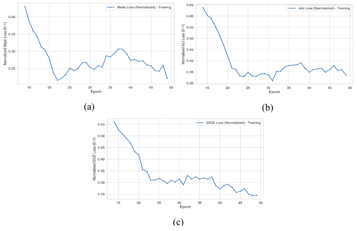
Figure 7.
(a) YOLOv8 based detections of spots in the operculum region, (b) YOLOv8 driven SAM-2 segmentations, (c) Final spots segmentation for features extraction and downstream analysis.
Figure 7.
(a) YOLOv8 based detections of spots in the operculum region, (b) YOLOv8 driven SAM-2 segmentations, (c) Final spots segmentation for features extraction and downstream analysis.
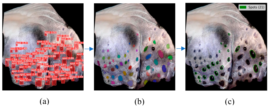
Figure 8.
(a) operculum grayscale image, (b) extracted spots through spots masks, (c) extracted background regions, (d,e) pre-and post-stress operculum regions with spot and background regions highlighted in green and red respectively.
Figure 8.
(a) operculum grayscale image, (b) extracted spots through spots masks, (c) extracted background regions, (d,e) pre-and post-stress operculum regions with spot and background regions highlighted in green and red respectively.
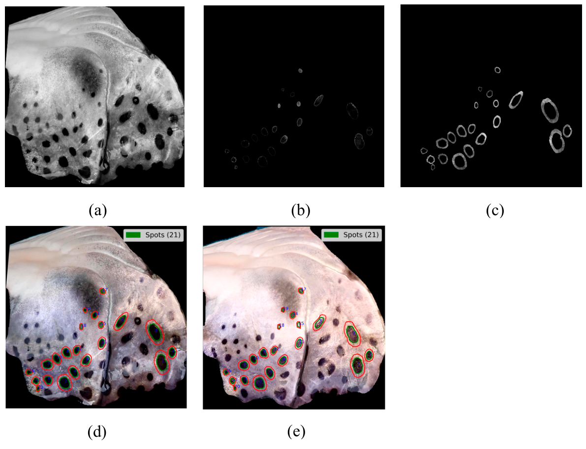
Figure 9.
Within-fish change in opercular spot features before and after 18 h confinement. Each grey line represents one operculum (n = 21 fish, left and right shown in separate rows); colored markers show group means ± SEM. Standardized effect sizes (d_z) are annotated. All four features changed significantly with day (p < 10⁻⁴), with no significant effect of side and no day × side interaction.
Figure 9.
Within-fish change in opercular spot features before and after 18 h confinement. Each grey line represents one operculum (n = 21 fish, left and right shown in separate rows); colored markers show group means ± SEM. Standardized effect sizes (d_z) are annotated. All four features changed significantly with day (p < 10⁻⁴), with no significant effect of side and no day × side interaction.
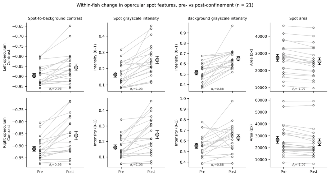
Figure 10.
Distribution of opercular spot features by session and side. Boxes show median and interquartile range with individual fish overlaid; whiskers extend to 1.5 × IQR. Left and right opercula are shown separately; the absence of a side effect is evident across all four features.
Figure 10.
Distribution of opercular spot features by session and side. Boxes show median and interquartile range with individual fish overlaid; whiskers extend to 1.5 × IQR. Left and right opercula are shown separately; the absence of a side effect is evident across all four features.
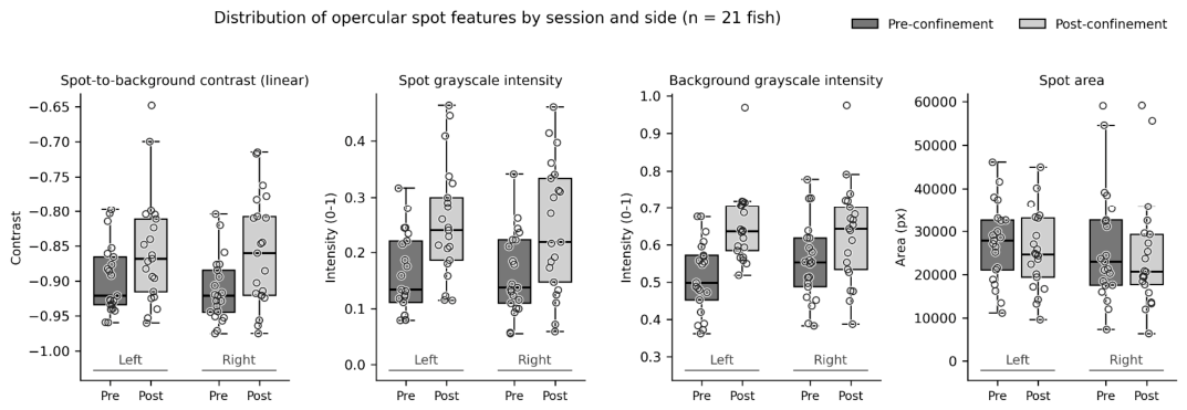
Figure 11.
Change in each feature plotted against change in log₂ sensor exposure between paired images. Lines show the fitted regression; the intercept of each is the exposure-adjusted effect reported in the text. No feature showed a significant dependence on exposure after normalization.
Figure 11.
Change in each feature plotted against change in log₂ sensor exposure between paired images. Lines show the fitted regression; the intercept of each is the exposure-adjusted effect reported in the text. No feature showed a significant dependence on exposure after normalization.
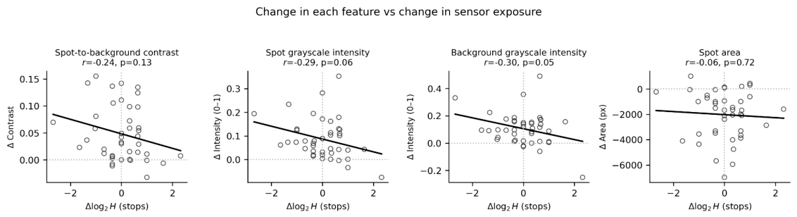
Figure 12.
Spot-to-background contrast in reference fish (n = 8), stressed fish before confinement (n = 21), and the same stressed fish after confinement (n = 21). Contrast is computed in linear light and is invariant to illumination scale and image magnification. Reference fish did not differ from pre-stress animals (p = 0.276) but differed from post-stress animals (Welch t-test, p = 0.002).
Figure 12.
Spot-to-background contrast in reference fish (n = 8), stressed fish before confinement (n = 21), and the same stressed fish after confinement (n = 21). Contrast is computed in linear light and is invariant to illumination scale and image magnification. Reference fish did not differ from pre-stress animals (p = 0.276) but differed from post-stress animals (Welch t-test, p = 0.002).
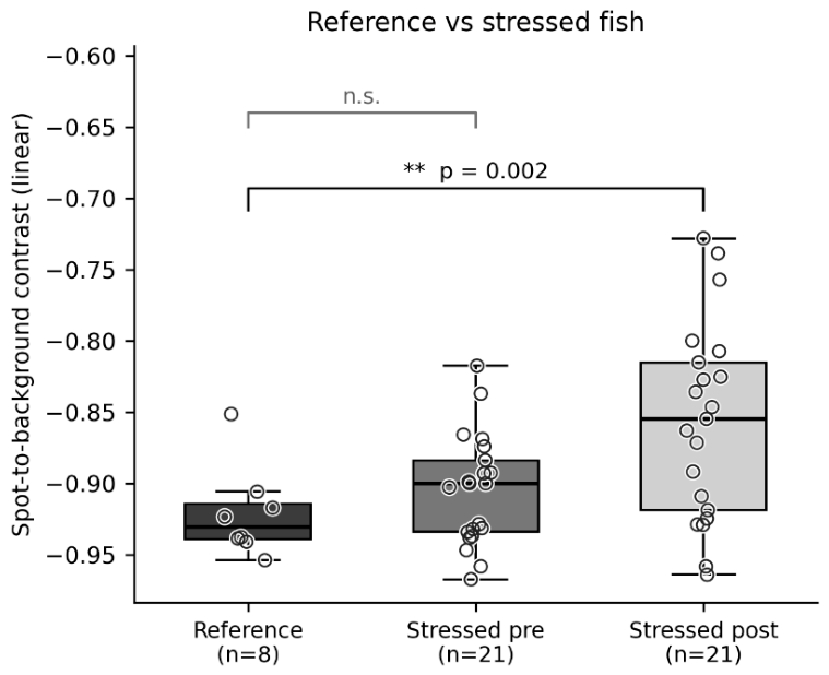

Table 1.
Positioning of the present study relative to prior work on melanin spot quantification and fish re-identification.
Table 1.
Positioning of the present study relative to prior work on melanin spot quantification and fish re-identification.
| Study | Subject | Tissue | Longitudinal | Individual spot resolution | Stressor tested | Illumination correction | Exposure normalization | Linear light normalization |
Effect size reported |
| Mathiassen et al. (2007) | Atlantic salmon | Fillet | No | Region-level | No | No | No | No | No |
| Saberioon et al. (2017) | Review | Various | - | - | No | No | No | No | No |
| Zhang et al. (2025) | Atlantic salmon | Fillet | No | Region-level | No | No | No | No | No |
| Gupta et al. (2022) | Atlantic salmon | Skin | No | Lesion-level | No | No | No | No | No |
| Cisar et al. (2021) | Atlantic salmon | Skin | Yes | Pattern-level | No | No | No | No | No |
| Bekkozhayeva et al. (2022) | Atlantic salmon | Scales | Yes | Pattern-level | No | No | No | No | No |
| Zhou et al. (2022) | Brook trout | Skin | Yes | Pattern-level | No | No | No | No | No |
| Laique et al. (2026) | Atlantic salmon | Operculum | Yes | Individual spot | Yes (18 h confinement) | Two-point luminance (eye/ID-tag) |
No | No | No (Proof of principle) |
| Present study | Atlantic salmon | Operculum | Yes | Individual spot | Yes (18 h confinement) |
Two-point luminance (eye/ID-tag) |
Yes (EXIF derived) | Yes |
Yes (adjusted with 95% CI) |
Table 2.
Training configuration.
| Parameter | Value |
| Base Architecture | YOLOv8x-seg |
| Pretrained Weights | MS-COCO (Lin et al., 2014) |
| Framework | Ultralytics |
| No. Of training images | 275 opercula; 1065 spots |
| Input resolution | 1080 x 1080px |
| Batch size | 4 |
| Maximum epochs | 100 |
| Early-stopping patience | 25 |
| Optimizer | Adam (Kingma & Ba, 2014) |
| Learning rate | 0.002 |
| Momentum (β1) | 0.99 |
| Dropuout | 20% |
| Augmentation | Albumentations: Gaussian blur, CLAHE, grayscale, tile-size |
Table 3.
Operculum segmentation performance of the fine-tuned YOLOv8-x (YOLOv8-seg) model across the training, validation, and test splits.
Table 3.
Operculum segmentation performance of the fine-tuned YOLOv8-x (YOLOv8-seg) model across the training, validation, and test splits.
| Model | Precision (Bbox) | Recall (Bbox) | Precision (Mask) | Recall (Mask) |
mAP50 (Mask) |
mAP50-95 (Mask) |
| Training | 0.95 | 0.97 | 0.95 | 0.97 | 0.995 | 0.796 |
| Validation | 0.998 | 1.00 | 0.998 | 1.00 | 0.99 | 0.76 |
| Testing | 0.998 | 1.00 | 0.998 | 1.00 | 0.995 | 0.7 |
Notes: Metrics are reported for the fine-tuned YOLOv8-x operculum segmentation model. Precision, recall, and mean average precision (mAP) at IoU 0.50 (mAP50) and across IoU 0.50–0.95 (mAP50–95) were computed from bounding boxes and masks against the ground-truth annotations. The model was trained on a single class (operculum region of interest).
Table 4.
Spot segmentation performance of the fine-tuned YOLOv8-x (YOLOv8-seg) models across the training, validation, and test splits.
Table 4.
Spot segmentation performance of the fine-tuned YOLOv8-x (YOLOv8-seg) models across the training, validation, and test splits.
| Model | Precision (Bbox) | Recall (Bbox) | Precision (Mask) | Recall (Mask) |
mAP50-95 (Bbox) |
mAP50-95 (Mask) |
|
| Training | 0.91 | 0.89 | 0.89 | 0.84 | 0.61 | 0.53 | |
| Validation | 0.934 | 0.917 | 0.916 | 0.881 | 0.643 | 0.588 | |
| Testing | 0.93 | 0.898 | 0.9 | 0.869 | 0.621 | 0.494 |
Table 5.
Training configuration.
| Parameter | Value |
| Base checkpoint | SAM 2.1 Hiera-B+ (Ryali et al., 2023; Ravi et al., 2024) |
| Input resolution | 1024 x 1024 px |
| Epochs | 50 |
| Batch size | 2 |
| Samples per batch | Single frame, ≤ 3 objects per image |
| Modules trained | Image encoder, memory attention, memory encoder |
| Optimizer | AdamW |
| Precision | Mixed (AMP) |
| LR schedule | Cosine |
| Base learning rate | 5 x 10⁻⁶ |
| Image-encoder learning rate | 3 x 10⁻⁶ |
| Layer-wise LR decay | 0.90 |
| Loss | Mask + Dice + IoU + object classification (mask weighted highest) |
| Prompt sampling | Point and box, equal probability |
| Augmentations | Horizontal flip, affine, resize, colour jitter, grayscale, ImageNet normalisation |
Table 6.
IoU and Dice metrics on held-out test set.
| Method Type | IoU Mean | IoU STD | DICE Mean | DICE STD | Spot Instances |
| Otsu | 0.6932 | 0.2108 | 0.7975 | 0.1729 | 832 |
| Adaptive | 0.6711 | 0.2195 | 0.7779 | 0.1952 | 832 |
| SAM 2 (Bbox) | 0.8151 | 0.0954 | 0.8948 | 0.0639 | 832 |
| SAM 2 (Point) | 0.7711 | 0.1324 | 0.8635 | 0.0985 | 832 |
Disclaimer/Publisher’s Note: The statements, opinions and data contained in all publications are solely those of the individual author(s) and contributor(s) and not of MDPI and/or the editor(s). MDPI and/or the editor(s) disclaim responsibility for any injury to people or property resulting from any ideas, methods, instructions or products referred to in the content. |
© 2026 by the authors. Licensee MDPI, Basel, Switzerland. This article is an open access article distributed under the terms and conditions of the Creative Commons Attribution (CC BY) license.
Copyright: This open access article is published under a Creative Commons CC BY 4.0 license, which permit the free download, distribution, and reuse, provided that the author and preprint are cited in any reuse.