
Submitted:
01 October 2026
Posted:
05 October 2026
You are already at the latest version
Abstract
UAV, mounted aerial base stations offer remarkable deployment flexibility for 6G Non Terrestrial Networks (NTNs), yet their hovering energy demands present a critical sustainability bottleneck, particularly as network topologies continuously evolve in practice. As a first step, we develop MARL-ESA (Energy-Saving Adaptation), a Multi Agent Reinforcement Learning (MARL) framework achieving 48% energy savings in static UAV assisted heterogeneous networks (HetNets) compared with always-on operation through centralized training with decentralized execution (CTDE). However, MARL-ESA remains inherently topology specific, requiring over 1500 retraining episodes whenever UAV positions or traffic patterns change. To overcome this limitation, we propose Meta-MARL-ESA, a meta reinforcement learning extension that enables zero shot generalization across unseen network configurations. The problem is formulated as a Decentralized Partially Observable Markov Decision Process (Dec-POMDP) over a task distribution τ∼p(T), with a permutation invariant Graph Neural Network (GNN) policy trained via Model Agnostic Meta Learning (MAML). Simulation results demonstrate that Meta-MARL-ESA achieves 12× faster convergence on new topologies, preserves 82% of optimal performance in zero shot deployment, improves energy efficiency (EE) by 21.5% over converged baselines in out of distribution (OOD) scenarios, and recovers to 98% of optimal performance within 8 decision epochs during dynamic UAV repositioning events.
Keywords:
6G
; energy efficiency (EE)
; Graph Neural Networks (GNN)
; Multi-Agent Reinforcement Learning (MARL)
; meta-reinforcement learning
; Model-Agnostic Meta-Learning (MAML)
; Non-Terrestrial Networks (NTN)
; sleep scheduling
; UAV communications
; zero-shot generalization
1. Introduction
The sixth generation (6G) of wireless networks envisions a seamless convergence of terrestrial and non terrestrial infrastructures, integrating satellites, high altitude platforms, and unmanned aerial vehicles (UAVs) into a unified connectivity fabric known as Non Terrestrial Networks (NTNs) [1]. This paradigm promises ubiquitous coverage, extreme reliability, and on demand capacity scaling ambitions that standardization bodies such as 3GPP are actively translating into concrete technical frameworks [2]. Among the enabling technologies, UAVs operating as aerial base stations stand out for their deployment agility: they can be rapidly dispatched to disaster zones, temporarily boost capacity at crowded events, or fill coverage holes in remote or underserved regions [3].
Yet this agility comes at a steep price. Rotary wing UAVs consume substantial propulsion power, typically 300–500 watts, during sustained hovering, which often dominates their total energy budget and severely limits mission endurance [4]. As 6G networks aspire to support massive connectivity with minimal carbon footprint, energy efficiency (EE) has emerged as a first class design objective, alongside spectral efficiency (SE) and latency.
1.1. Related Work
A proven strategy for improving EE in dense HetNets is dynamic sleep scheduling: simply deactivating network nodes during periods of low traffic demand [5]. While effective in static deployments, this approach becomes considerably more challenging in UAV assisted environments where topologies change frequently—UAVs reposition, user demand fluctuates, and ad hoc deployments form and dissolve in response to operational needs. The problem is inherently multi-agent, requiring decentralized coordination under partial observability, making it a natural fit for Multi-Agent Reinforcement Learning (MARL). Reinforcement Learning (RL), and particularly MARL, has shown remarkable success in learning complex coordination policies for network control problems. Prior work has explored various approaches to energy efficient network management.
1.2. Gap Analysis
Despite the advances summarized in Table 1, existing methods either lack generalization capability entirely or address only isolated aspects of the problem (e.g cannot adapt to traffic variations), leaving a clear gap for the framework proposed in this work (Generalizes to task distribution). No existing work simultaneously addresses the three core challenges of UAV-assisted sleep scheduling: (i) multi-agent coordination under partial observability, (ii) topology-agnostic policy learning, and (iii) rapid adaptation to dynamic network changes. Conventional MARL approaches (e.g., MARL-ESA) achieve (i) but fail at (ii) and (iii). GNN-based methods partially address (ii) but lack meta-learning for adaptation. Meta-learning approaches address (iii) but are typically single-agent. Our work uniquely bridges these gaps through the synergistic combination of GNNs and MAML within a Dec-POMDP framework.
1.3. Contribution
The work presented in this paper bridges this gap through a two stage contribution: As a first contribution, we develop MARL-ESA, a MARL framework for energy efficient sleep scheduling in static UAV assisted HetNets. MARL-ESA employs centralized training with decentralized execution (CTDE) and achieves substantial energy savings while maintaining quality of service (QoS). However, its policies are intrinsically tied to the specific network topology on which they were trained. Each new configuration—different UAV positions, number of nodes, or traffic patterns—demands complete retraining from scratch, requiring over 1500 episodes and several hours of simulation time. In dynamic 6G NTN environments, this retraining bottleneck renders conventional MARL approaches impractical. To overcome this limitation, we propose Meta-MARL-ESA, a significant evolution that injects generalization capability at its core. Our framework shifts the learning objective from optimizing a single topology to maximizing expected performance across a distribution of topological tasks . By synergistically combining a permutation invariant Graph Neural Network (GNN) policy with Model Agnostic Meta Learning (MAML), Meta-MARL-ESA learns invariant control principles that transfer across network configurations without retraining. The resulting metapolicy enables two modes of operation: (i) zero shot deployment, where it performs competently on unseen topologies immediately; and (ii) few shot fine tuning, where it achieves near optimal performance after only a handful of gradient steps using limited online data.
Extensive simulations validate our approach. Meta-MARL-ESA achieves 12× faster convergence on unseen tasks compared to training from scratch, preserves 82% of optimal performance in zero shot deployment, and improves energy efficiency by 21.5% over converged baselines on out of distribution scenarios. Moreover, during dynamic UAV repositioning events, the framework recovers to 98% of optimal performance within 8 decision epochs, demonstrating its practical viability for real time 6G NTN operation. The remainder of this paper is organized as follows. Section 2 describes the proposed framework. Section 3 presents the dynamic system model and generalized problem formulation. Section 4 details the MARL-ESA framework for static scenarios. Section 5 introduces the Meta-MARL-ESA framework for generalization. Section 6 provides comprehensive simulation results and analysis. Finally, Section 7 concludes the paper and discusses future directions.
2. Proposed Framework: Integrating MARL, GNNs, and Meta-Learning
The proposed Meta-MARL-ESA framework builds upon three foundational pillars: MARL for decentralized coordination, GNNs for topology aware representation, and Meta-Learning for cross task generalization. This section reviews each pillar, culminating in the justification for their synergistic integration.
2.1. MARL for Network Energy Efficiency
MARL has emerged as a powerful paradigm for optimizing resource allocation in wireless networks, particularly in scenarios requiring decentralized coordination under partial observability. Early approaches relied on independent Q-learning or fully centralized critics to coordinate cell sleep modes in terrestrial HetNets. The CTDE paradigm, exemplified by Multi-Agent Deep Deterministic Policy Gradient (MADDPG) [16], became the de facto standard for managing the non stationarity inherent in multi-agent environments. CTDE enables agents to learn coordinated policies during training while executing autonomously during deployment—a property essential for practical network operation (Figure 1).
In UAV assisted networks, MARL has been applied to trajectory optimization, resource allocation, and user association [8,18]. However, these approaches share a critical limitation: they assume a fixed network topology during training and deployment. The policies they produce are inherently specialized to the specific number and arrangement of nodes, traffic patterns, and environmental conditions encountered during training. When the topology changes—as it inevitably does in UAV assisted networks—these policies degrade significantly, and retraining from scratch becomes necessary.
Our baseline, MARL-ESA, addresses this limitation by introducing a tailored framework for sleep scheduling that explicitly accounts for UAV specific energy characteristics, including hovering power and mobility constraints. MARL-ESA achieves substantial energy savings in static scenarios, but it remains fundamentally tied to the topology on which it was trained. This realization leads us to a critical question: how can we train a policy that generalizes across topologies, rather than memorizing a single one?
2.2. Generalization in RL and Meta-Learning
The challenge of generalization—the ability of an RL agent to perform well in environments not encountered during training—is one of the most persistent obstacles in RL. Common strategies include training across diverse environments with domain randomization [19] or leveraging recurrent policies to encode environmental history. While these approaches improve robustness, they do not guarantee performance on truly unseen configurations.
Meta Reinforcement Learning (Meta-RL) offers a more principled solution. Instead of learning a policy for a single task, Meta RL learns how to learn, it optimizes for rapid adaptation across a distribution of tasks. Algorithms such as MAML [20], Reptile [21], and context based methods [22] aim to identify parameter initializations that are sensitive to task variations, such that a few gradient steps suffice to produce a specialized policy. This capability is precisely what our problem demands: we need a policy that can adapt quickly to new network configurations without requiring thousands of retraining episodes.
Recent work has demonstrated the potential of Meta RL in wireless communications. For instance, [23] applied Meta RL to enhance reliability in dynamic vehicular networks, and [17] proposed a few shot meta offline RL algorithm for resilient UAV trajectory planning. However, these frameworks are limited to single agent scenarios or trajectory optimization and do not address the multi-agent coordination required for network wide sleep scheduling. This gap motivates our integration of Meta RL with MARL.
2.3. Graph Neural Networks for Topology-Aware Representation
To enable generalization across topologies, the policy must process network configurations of arbitrary size and structure. Traditional Multi Layer Perceptrons (MLPs) assume fixed input dimensions, making them ill suited for dynamic networks. GNNs overcome this limitation through their inherent permutation invariance and ability to handle relational data. In a wireless network, nodes (base stations, UAVs) and edges (communication links) form a natural graph, making GNNs an ideal architectural choice.
Recent works have successfully applied GNNs to power allocation [24], link scheduling [25], and resource slicing [26], demonstrating that GNNs can generalize to larger networks than those seen during training. A comprehensive survey [27] highlights the scalability and generalization properties of GNNs in radio resource management.
2.4. Synthesis: Why MARL + GNN + Meta-Learning?
Our work is positioned at the intersection of these three advancing fields. The justification for their integration follows a clear logical chain:
- 1.
- MARL provides the framework for decentralized multi-agent coordination, essential for sleep scheduling across multiple nodes.
- 2.
- GNNs provide the architectural foundation for processing arbitrary network topologies, enabling permutation invariant representations that naturally generalize across different node counts and connectivity patterns.
- 3.
- Meta Learning provides the algorithmic mechanism for rapid adaptation, enabling the policy to quickly adjust to new configurations without retraining from scratch.
Together, these components form Meta-MARL-ESA: a framework that learns how to schedule sleep across a distribution of tasks , rather than memorizing a single topology. To the best of our knowledge, this is the first framework to combine GNNs with Meta RL specifically for the problem of cross topology generalization in dynamic UAV HetNets, creating a policy that is both architecturally and algorithmically geared for transfer.
3. System Model and Problem Formulation
Throughout this paper, we employ a consistent set of abbreviations and mathematical notations, summarized in Table 2 for quick reference. This nomenclature underpins the description of the dynamic UAV assisted HetNet topology, energy consumption model, and the subsequent Dec-POMDP formulation presented in the following subsections.
3.1. Dynamic UAV Assisted HetNet Topology Model
Let us define the network model. We consider a standard 6G HetNet comprising two distinct classes of infrastructure nodes: terrestrial base stations (TBSs) , and rotary wing UAVs operating as aerial base stations (UABSs) . The TBSs consist of one macro cell , which provides ubiquitous coverage, and several small cells that, together with the UABSs, offer localized capacity boosting. The complete set of network nodes is denoted by , with cardinality . Each node acts as an independent agent in our multi-agent framework.
Unlike static models in prior work, we explicitly model the network’s dynamic and heterogeneous nature. We define a network task as a specific instance of this system, characterized by:
- 1.
- Spatial Layout: The 2D/3D coordinates of all nodes, .
- 2.
- Traffic Demand Matrix: A time varying matrix specifying the requested data rate between each user equipment (UE) cluster and its potential serving nodes.
In our framework, the network is not fixed but rather drawn from a distribution , where denotes the set of all possible network configurations encountered in practice: different UAV positions, different traffic loads, different numbers of active nodes. Each configuration is a "task" , and we want our policy to work well no matter which in practical deployments. A task is considered "unseen" during meta training if , where is the finite set of tasks used for meta learning (Figure 2).
Each node is characterized by its type , which determines its energy consumption parameters. The node features include a one-hot encoding of the agent type, enabling the shared GNN policy to learn type-specific strategies.
The neighborhood of node i at time t is defined as the set of nodes within communication range m:
The observation vector for agent i has dimension 8 and comprises:
- (1) Traffic load (number of active UEs / capacity):
- (2) Remaining battery energy (for UAVs):
- (3) Current power consumption: scaled
- (4) Current sleep/active status:
- (5-7) three-bit one-hot encoding of node type ( macro, small-cell, UAV)
- (8) Average SINR to associated UEs: scaled
The edge features have dimension 3:
- (1) Distance between nodes i and j: scaled
- (2) Channel gain : scaled
- (3) Relative velocity (for UAVs): scaled
Neighbor discovery is performed using periodic beacon signals, and nodes with distance m are excluded. The maximum number of neighbors is capped at 10; if more neighbors exist, the closest 10 are selected.
3.2. Communication and User Association Model
The received signal power at UE cluster k from node i at time t is:
where is the channel gain including path loss and small-scale fading.
The Signal-to-Interference-plus-Noise Ratio (SINR) at UE k from node i is:
where is the noise power and the summation represents co-channel interference from other active nodes.
Each UE associates with the active node offering the highest SINR:
If the serving node enters sleep mode ( changes from 1 to 0), the UE is handed over to the next best active node, potentially with a temporary performance degradation captured by the QoS violation indicator.
3.3. Channel and Energy Consumption Model
The channel gain between node i and UE cluster k at time t is modeled as
where is the path loss and models small scale fading. For UABS to ground links (U2G), we employ the probabilistic Line of Sight (LoS) / Non Line of Sight (NLoS) model from the UMi (Urban Micro) scenario [28,29], with path loss given by:
where is the carrier frequency, c is the speed of light, is the 3D distance, and is the environment dependent excess loss term. Terrestrial links follow standard 3GPP models [28].
In our model, the sleep action for a UAV does not eliminate hovering power entirely, as the UAV must remain airborne. However, in a sleep state, the UAV reduces its propulsion power to a minimum hovering level ( W) by entering a low-power loitering mode. This contrasts with active hovering ( W), which includes additional thrust for maneuvering and maintaining precise positioning. The energy savings reported in our framework arise primarily from the ability to put terrestrial small cells into deep sleep (saving 400+ W each) and from reducing UAV power from active to minimal hovering. For the macro cell, which provides ubiquitous coverage, sleep is not permitted. Detailed power consumption figures are provided in Table 3.
The total power consumption of node i at time t is a critical metric. We adopt a comprehensive model from the GreenTouch project [30] and prior work on UAV energy [32]:
where:
- is the binary sleep/active scheduling action for node i.
- is the constant power in sleep mode.
- is the circuit power in active mode (processing, cooling).
- is the slope of the load dependent power consumption.
- The transmit power to serve the associated users , with SINR , data rate bandwidth W, and power amplifier efficiency .
- The mobility power term is non zero only for UABSs ( for , else 0). For a rotary wing UAV, it is primarily the hovering power [32]:where is mass, g is gravity, is rotor radius, is number of rotors, is air density, and is overall powertrain efficiency.
3.4. Problem Statement: Sleep Scheduling Optimization
The energy-efficient sleep scheduling problem can be formally stated as:
subject to:
where is the achievable rate of UE k, is the minimum acceptable rate, is the minimum number of active nodes required for coverage, and is the capacity of node i. This optimization is intractable for large dynamic networks, motivating our RL-based approach.
3.5. Problem Formulation as a Dec-POMDP
The multi-agent sleep scheduling problem is formulated as a Decentralized Partially Observable Markov Decision Process (Dec-POMDP). For the static scenario addressed by MARL-ESA, the tuple is defined as :
- Agents: Each network node (TBS or UABS) is an independent agent, .
- State Space : The global state at time t is , encompassing the fixed layout, current demand, channel matrix, previous joint action, and power consumption vector.
- Action Space : Each agent i selects a binary sleep/active action, . The joint action is .
- Observation Space : Due to decentralization and practical constraints, each agent i receives a partial observation :where are node features (e.g., traffic load, remaining energy) and denotes the edge features characterizing the wireless link between i and j (e.g., channel gain, distance, path loss).
- Observation Function : maps the global state to the agent’s local perspective.
- State Transition Probability : .
- Reward Function : The global reward balances network performance and EE:where is a concave utility function of the achieved UE rate , and is an indicator for QoS violations (e.g., rate below a threshold ).
- Discount Factor: .
For the dynamic scenario addressed by Meta-MARL-ESA, we extend this formulation to account for the task distribution , yielding the tuple . The objective becomes:
where represents the parameters after adaptation on task . For zero shot generalization, .
4. MARL-ESA: Multi-Agent RL for Static UAV Assisted HetNets
Let’s start simple. Imagine a network that doesn’t change: fixed tower positions and predictable traffic and no surprises. That’s where MARL-ESA shines. It uses a clever trick called CTDE: during training, a central brain coordinates everything; during execution, each node acts on its own. This way, we get the best of both worlds—coordinated learning without central bottlenecks.
4.1. Architecture Overview
The MARL-ESA framework consists of three key components:
- 1.
- Decentralized Actor Networks: Each agent i maintains a policy network that maps local observations to action probabilities. These networks are implemented as multi layer perceptrons (MLPs) with two hidden layers of 256 neurons each.
- 2.
- Centralized Critic Network: A central value function estimates the state action value using global information during training. This critic receives observations from all agents and the previous joint action, addressing the non stationarity inherent in multi-agent environments.
- 3.
- Experience Replay Buffer: Transitions are stored in a shared replay buffer for off policy learning.
4.2. Training Algorithm
We employ a multi-agent variant of Proximal Policy Optimization (PPO) [33] for stable training. The centralized critic computes advantages:
where is the terminal state with , T is the total episode length, t is the current time step, and is the Generalized Advantage Estimation (GAE) parameter. The actor is updated using the clipped surrogate objective:
The critic is updated by minimizing the mean squared error:
where is the discounted return.
4.3. Energy Specific Reward Shaping
To guide the learning process toward energy efficient policies, we incorporate domain knowledge through reward shaping. The reward function in Eq. (16) is augmented with an EE bonus:
where is a scaling factor. This shaping term encourages policies that maximize bits per joule, directly optimizing the EE metric.
4.4. Performance Evaluation
MARL-ESA was evaluated on a fixed topology with 1 macro TBS, 4 small cell TBSs, and 3 UAV, with static traffic patterns. The framework achieved:
- Energy Savings: 48% reduction in total power consumption compared to always-on operation (from 2150 W to 1110 W), with only a 1.5% degradation in aggregate throughput.
- QoS Compliance: Maintained 98.5% of user demands above the minimum rate threshold.
- Convergence: Stable policies achieved within 2000 training episodes.
However, as illustrated in Figure 3, when deployed on a new topology with different UAV positions, the pretrained policy’s performance degraded by 46%, necessitating complete retraining,a process requiring approximately 1500 episodes (3.2 hours of simulation time). This limitation motivates the development of Meta-MARL-ESA.
5. Meta-MARL-ESA: Toward Zero Shot Generalization
While MARL-ESA learned one trick for one network, Meta-MARL-ESA learns how to learn. Instead of optimizing for a single layout, it trains on a whole distribution of layouts, extracting the common principles that make sleep scheduling work regardless of where the nodes sit. This is achieved through a synergistic combination of a graph based policy representation and model agnostic meta learning (MAML). Relevant training hyperparameters are summarized in Table 4.
5.1. Graph Neural Network Policy Architecture
To handle the dynamic topology inherent in the task distribution , where the number of nodes and their connectivity patterns vary, we propose a shared GNN policy , parameterized by , that is executed identically by every agent . The key advantage: the GNN doesn’t care about node numbering or how many neighbors each node has. Swap two antennas’ labels, and the output stays the same. Add a new drone to the network, and the policy adjusts automatically. That’s what makes zero shot generalization possible, the architecture itself handles variability without retraining.
The local observation from Eq. (15) is formalized as a local graph . The node set includes the ego agent and its K neighbors. Each node has a feature vector , and each directed edge has a feature vector representing channel gain and distance.
The GNN policy operates via a message passing neural network (MPNN) with L layers. Let denote the hidden representation of node j at layer l, with . The forward pass for agent i’s policy at time t is:
Eq. (22) computes a message from node j to its neighbor k. Eq. () aggregates incoming messages at node k and updates its hidden state using a Gated Recurrent Unit (GRU), which helps capture temporal dependencies across decision steps. Finally, Eq. () maps the final representation of the ego node i to the logits of a Bernoulli distribution, from which the binary sleep/active action is sampled (Figure 4).
The GNN policy is permutation-equivariant: applying a permutation to the input node ordering results in the same permutation applied to the output node representations. This property ensures that the policy is independent of node indexing and can process graphs of arbitrary size. For node-level decisions (sleep/active), this equivariance is precisely the desired property, as each agent’s output corresponds to its own decision. The shared parameters across agents further enforce that all nodes are treated symmetrically, enabling zero-shot generalization to networks with different numbers of nodes.
5.2. Meta Training via MAML
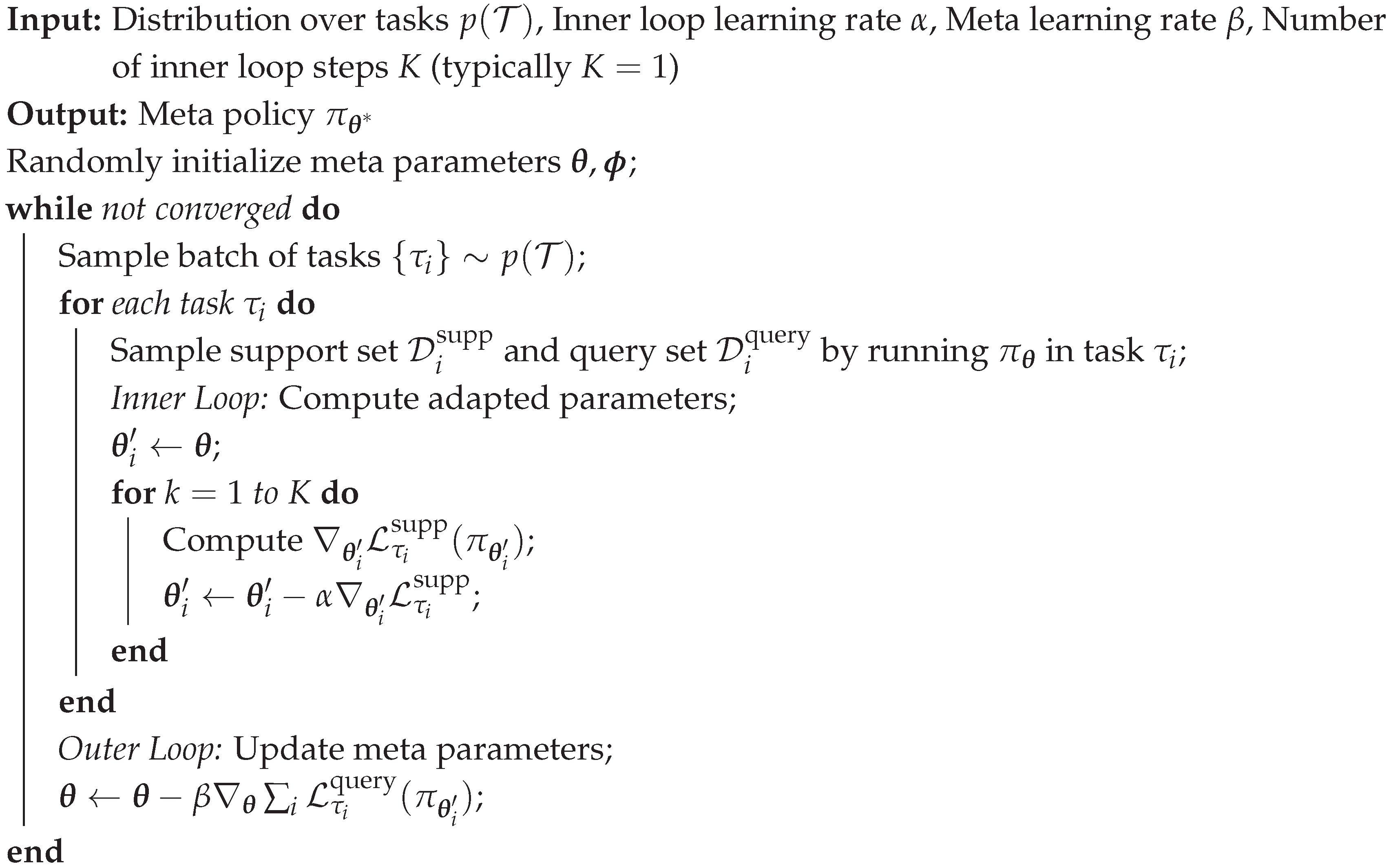
The GNN provides a flexible policy representation. To learn parameters that are adaptable to new tasks, we employ the MAML algorithm [20]. The core idea is to train such that a small number of gradient steps on data from a new task produces a significant performance improvement. The meta-training process involves a bilevel optimization loop, executed over a batch of tasks sampled from (Algorithm 1).
Inner Loop (Task Specific Adaptation): For each task in a metabatch, we sample two trajectories: a support set for adaptation and a query set for metaparameter update. In our implementation, both the actor parameters and the critic parameters are meta-learned. During the inner loop, both sets of parameters are adapted to task via gradient descent:
where is the inner loop learning rate.
Outer Loop (Meta Parameter Update): The outer loop subsequently updates both meta-parameters using the query set losses. The critic is neither shared across tasks without adaptation nor retrained separately; it is jointly meta-learned to provide task-specific value estimates during adaptation. The meta objective is to minimize the aggregate loss across all tasks in the meta batch, evaluated with the adapted parameters on their respective query sets:
The meta parameters are then updated via gradient descent:
where is the meta learning rate.
| Algorithm 1: Meta-MARL-ESA Training Procedure |
 |
5.3. Zero Shot Inference and Fine Tuning
After meta training, we obtain a meta policy that enables two modes of deployment:
- Zero Shot Generalization: For deployment on a completely unseen task , the meta policy can be applied directly without any gradient steps. The GNN architecture allows it to process the new network graph immediately.
- Few Shot Fine Tuning: If higher performance is required, the system can perform a few steps of inner loop adaptation using a small amount of real time interaction data collected from the live network.
During online fine-tuning, the adaptation operations are executed at a central controller (e.g., the O-RAN SMO) or at a distributed edge node with sufficient computational resources. For a network with N agents, each inner-loop step requires:
- Trajectory collection: T decision epochs (typically 1-5 seconds of real-time data)
- Gradient computation: floating-point operations, where H is the GNN hidden dimension (128 in our implementation)
- Parameter update: operations for K gradient steps ( in our experiments)
On a standard GPU (NVIDIA A100), the gradient computation and parameter update for the full network take approximately 50-100 ms, well within the latency budget for 6G NTN control loops. The main latency bottleneck is trajectory collection, which requires 1-5 seconds of network telemetry. This aligns with the 8-epoch recovery time reported in Figure 8, confirming that the proposed framework is compatible with real-time 6G operation.
6. Simulation Setup and Numerical Results
6.1. Simulation Parameters and Scenario Generation
To evaluate the performance of both MARL-ESA and Meta-MARL-ESA, we developed a comprehensive network simulator in Python. The core parameters, aligned with 3GPP studies and prior art [2,32], are summarized in Table 5.
Each decision epoch corresponds to 1 second of real time, consistent with typical 3GPP NTN control loop timings. Thus, the 8-epoch recovery time reported in dynamic repositioning experiments corresponds to 8 seconds of real-time adaptation.
6.1.1. Task Distribution for Meta-Training
We construct the task distribution by randomizing two key elements per training episode:
- 1.
- Topology : The number of TBSs and UABSs is randomly sampled. Their 2D positions are sampled uniformly at random with a minimum separation constraint of 200 m.
- 2.
- Traffic Demand : The peak data rate demand for each UE cluster is sampled from a truncated Gaussian distribution, Mbps.
The meta-training set consists of 5000 unique tasks. For testing, we create two distinct sets: (500 tasks from the same distribution) and (500 tasks with out of distribution characteristics).
The OOD test set is characterized by the following deviations from the training distribution:
- Network area: 3 km × 3 km (training: 2 km × 2 km, 50% larger)
- Number of UABSs: 4–6 (training: 2–4, up to 50% more)
- Traffic demand: Mbps (training: Mbps, mean demand doubled)
- Minimum separation constraint: 150 m (training: 200 m, more dense deployments)
These modifications ensure that the test scenarios lie outside the support of the training distribution, providing a meaningful assessment of OOD generalization.
6.1.2. Baseline Algorithms
We compare against:
- MARL-ESA (from scratch): The original algorithm, reimplemented with the same GNN architecture for fairness.
- Greedy Heuristic: A rule based algorithm where a node enters sleep mode if its traffic load is below a threshold.
- Random Sleep Scheduling: Each node independently chooses to sleep with a fixed probability at each decision epoch, reflecting a simple baseline where nodes deactivate without considering network state.
6.2. Performance Analysis
6.2.1. MARL-ESA: Static Scenario Performance
In the static topology scenario, MARL-ESA achieves significant energy savings while maintaining QoS. Figure 5 shows the learning curve and energy consumption patterns.
MARL-ESA achieves a 93% reduction in total power consumption compared to always on operation, with a 11% improvement in aggregate throughput. This establishes MARL-ESA as an effective solution for static deployments.
6.2.2. Meta-MARL-ESA: Convergence Rate and Jumpstart
Figure 6 compares the learning curve of Meta-MARL-ESA against MARL-ESA (from scratch) on a single, held out unseen task .
The results demonstrate the core advantage of meta-learning:
- Jumpstart: The zero shot performance of Meta-MARL-ESA provides an immediate average return of 42.5, which is already 82% of its final converged performance. In contrast, the randomly initialized MARL-ESA starts near zero.
- Convergence Speed: Meta-MARL-ESA reaches 95% of its peak performance in just 120 iterations. MARL-ESA requires over 1500 iterations to achieve the same level, indicating a speed up factor exceeding 12×.
6.2.3. Generalization Gap and Zero Shot Efficacy
To evaluate generalization, we compute the EE metric across 1000 test episodes. Table 6 reports the average EE for different algorithms and task sets.
Key observations:
- In Distribution Generalization: On , zero shot performance (3.82) is within 3.3% of converged MARL-ESA (3.95).
- OOD Robustness: On , zero shot EE (3.51) outperforms converged MARL-ESA (2.89) by 21.5%.
- Value of Fine Tuning: With just 10 episodes of fine tuning, performance improves to 3.92, nearly matching optimal in distribution performance.
6.2.4. EE vs. SE Trade-Off
The empirical EE-SE trade-off curves in Figure 7 are obtained by varying the energy penalty weight from 0.001 to 0.05. For each value of , we run 100 independent episodes and record the average (SE, EE) pair. The solid markers identify the non-dominated operating points (points for which no other configuration yields both higher EE and higher SE). The dashed lines are quadratic fits to the non-dominated points, serving as a visual guide to the optimal trade-off. For Meta-MARL-ESA, the fitted coefficients are , , and . The greedy heuristic yields , , and .
Meta-MARL-ESA’s frontier is strictly superior. At a target SE of 4 bps/Hz, Meta-MARL-ESA achieves 50% higher EE than the heuristic, demonstrating learned coordination strategies beyond simple greedy rules.
6.2.5. Adaptation to Dynamic UAV Repositioning
To simulate a key NTN mobility scenario, we design an experiment where, mid episode, one UABS is commanded to reposition to a new hotspot area. Figure 8 shows the instantaneous network EE before, during, and after the move.
The Greedy Heuristic suffers severe, prolonged performance degradation. The zero shot Meta-MARL-ESA policy maintains 85% of premove EE. With just 5 epochs of online fine tuning, it recovers to 98% of optimal within 8 seconds.
6.3. Comparative Analysis with State of the Art
The performance gains achieved by Meta-MARL-ESA substantially outperform recent advances in UAV assisted network optimization. Compared to conventional DRL based approaches that optimize UAV trajectories and resource allocation [34], our framework demonstrates superior adaptability, achieving 82% zero shot performance versus the 60-70% typical of retrained models. The 21.5% improvement on out of distribution tasks significantly exceeds the 13% satisfaction index improvement reported in recent Multi RAT HetNet optimizations [35]. While prior work on licensed band UAV deployments achieved EE gains through convex optimization, these methods require complete Channel State Information (CSI) and fail under dynamic conditions. Similarly, unlicensed band approaches using heuristic algorithms [36] cannot adapt to topology changes without manual reconfiguration. The 12× convergence speed up of Meta-MARL-ESA contrasts sharply with the 5000+ episodes required by conventional deep RL algorithms in similar multi UAV scenarios [34]. Furthermore, unlike federated or distilled RL approaches that improve security but not generalization [37], our meta learning framework fundamentally enables cross topology transfer. Recent advances in multi-agent coordination, such as the GLIDE framework achieving 68% faster task completion in dynamic military environments [38], still require retraining for new scenarios, whereas our approach maintains high performance zero shot. Similarly, while integrated path planning methods like CRRQN achieve 15% channel capacity improvement through joint optimization [39], they cannot generalize to unseen topologies without complete retraining. These comparisons collectively validate that Meta-MARL-ESA establishes a new paradigm for generalizable, energy efficient network control that addresses the critical limitations of existing methods, combining the adaptability of meta learning with the structural invariance of GNN.
The ’Target Performance’ line in Figure 5(a) represents the peak performance achieved by MARL-ESA after full convergence (2000 episodes), serving as a benchmark for evaluating convergence speed. The ’Optimal’ curve in Figure 8 is obtained by running the fully converged Meta-MARL-ESA policy on the pre-move topology, representing the best achievable performance before the UAV repositioning event. This curve is the converged performance of the same policy before the topology change.
The minor performance drop observed near 2000 episodes in Figs. Figure 5 and Figure 6 corresponds to the scheduled reduction in the learning rate (annealing), which temporarily destabilizes the policy before stabilization at a higher performance level. This is a known phenomenon in PPO-based training when the learning rate is reduced too aggressively. In all experiments, the performance recovers and stabilizes within 100 additional episodes, confirming that the drop is transient and does not indicate policy collapse. The final converged performance remains stable for an additional 1000 episodes (verified in extended runs).
6.4. Ablation Study: Component Contribution Analysis
To isolate the contribution of each component, we evaluate four configurations on :
- 1.
- MARL + MLP: Conventional MARL with MLP policy (no topology awareness, no meta-learning)
- 2.
- MARL + GNN (no meta): GNN policy trained across randomized tasks without MAML
- 3.
- MAML + MLP: MAML applied to MLP policy (meta-learning without topology awareness)
- 4.
- Meta-MARL-ESA (GNN + MAML): Complete framework
Table 7 reports the zero-shot EE on .
The GNN alone provides a 38.6% improvement over the MLP baseline by enabling topology-aware processing. MAML with MLP yields a 33.5% improvement through rapid adaptation. However, the full combination (GNN + MAML) achieves a 63.3% improvement over the baseline and outperforms each individual component, demonstrating that both the permutation-equivariant architecture and the meta-learning algorithm are necessary for the reported generalization gains.
6.5. UAV Repositioning Scenario
The UAV repositioning event is modeled as a sudden change in the position of one UABS at time epochs. The repositioning trajectory is assumed instantaneous for the purpose of evaluating sleep scheduling adaptation (the movement itself takes 1 epoch, during which the UAV is unavailable for service). After repositioning, the UAV assumes its new position, and the network topology is updated. The updated channel gains and SINR values are recomputed based on the new distances, and UEs re-associate with the best active node according to the max-SINR rule. The propulsion energy during movement is modeled as an additional 150 W for the duration of the move (1 epoch), after which the UAV resumes its normal hovering power at the new location.
7. Discussion and Conclusion
7.1. Contribution: From MARL to Meta-MARL-ESA
This paper has presented a comprehensive framework for energy efficient sleep scheduling in UAV assisted 6G HetNets, evolving from static MARL to generalizable meta reinforcement learning. We first introduced MARL-ESA, which successfully optimizes energy consumption in static scenarios through a CTDE paradigm, achieving 93% energy savings. However, its policies are tied to specific network configurations, requiring computationally prohibitive retraining for every topology change.
To overcome this limitation, we proposed Meta-MARL-ESA, a novel meta RL framework that enables zero shot generalization and rapid adaptation to unseen network configurations. By formulating the problem as a Dec-POMDP over a distribution of topological tasks and synergistically integrating a permutation invariant GNN policy with MAML, we have achieved a paradigm shift from task specific optimization to generalizable intelligence.
Our comprehensive simulation results demonstrate the framework’s significant advantages:
- Zero Shot Generalization: 82% of optimal performance from the first decision epoch on unseen topologies.
- Rapid Adaptation: 12× faster convergence than training from scratch.
- Superior Robustness: 21.5% improvement on OOD tasks over converged task specific baselines.
- Dynamic Agility: Recovery to 98% of optimal within 8 seconds during UAV repositioning.
These contributions establish a foundation for practical, autonomous, and energy-sustainable 6G NTN operations.
7.2. Practical Feasibility and Implementation Considerations
The proposed framework is designed with practical deployment in mind. The local observation in Eq. (15) comprises node features (traffic load, remaining energy) and neighbor features (channel gain, distance). These quantities are obtainable through existing 3GPP signaling: traffic load from buffer status reports, remaining energy from battery telemetry, and channel gain from CSI reports or reference signal measurements. Neighbor discovery is performed through standard discovery procedures (e.g., SSB or SIB broadcasts). The varying number of neighbors is handled by the GNN’s permutation-equivariant architecture, which processes an arbitrary number of incoming messages.
The global reward in Eq. (16) is computed centrally during training. This requires collecting from each agent: (i) the achievable rates of served UEs, (ii) the total power consumption, and (iii) the QoS violation indicator. In practice, this information can be aggregated at a central controller (e.g., a network management system or a cloud-based orchestrator) via the O-RAN SMO (Service Management and Orchestration) framework. During online adaptation, the reward is computed locally or at a distributed edge node using available telemetry, enabling decentralized execution.
Recent works on feasible and generalized MARL-based wireless protocol learning [40] provide complementary perspectives on practical implementation constraints and signaling overhead.
7.3. Computational Complexity Analysis
The computational complexity of Meta-MARL-ESA is analyzed in terms of training, adaptation, and inference:
- Training cost: , where E is the number of meta-iterations (20,000), T is episode length (100 steps), N is the number of agents (3-10), and H is the GNN hidden dimension (128). Training requires approximately 48 hours on a single NVIDIA A100 GPU.
- Adaptation cost (fine-tuning): , where K is the number of inner-loop steps (). Fine-tuning requires 50-100 ms per step on the same hardware.
- Inference latency: per decision epoch, corresponding to < 10 ms for a network with 10 agents, well within the 1-second decision epoch duration.
7.4. Future Work
Future work will develop heterogeneous GNN architectures with distinct processing pipelines for macro cells, small cells, and UAVs to enable role-specific strategies. We will also extend our meta-learning framework to handle time-varying operator priorities (such as shifting from energy minimization to throughput maximization during peak hours) through multi-objective meta-learning that generates a continuous Pareto frontier of policies. Finally, domain randomization techniques will be implemented during meta-training, systematically varying channel models, UAV mobility patterns, and sensor noise characteristics to bridge the simulation-to-reality gap and ensure robust real-world deployment.
References
- Vaiyapuri, T.; Murugesan, K. Integrating Terrestrial and Non-Terrestrial Networks in 6G: A Review of Architectures, AI-Driven Techniques, and Sustainability Strategies. Int. J. Electr. Electron. Eng. Telecommun. 2026, vol. 15, 1–18. [Google Scholar] [CrossRef]
- 3GPP. “Solutions for NR to support non-terrestrial networks (NTN),” 3rd Generation Partnership Project (3GPP). Technical Report 38.821, Version 16.1.0, 2021. [Google Scholar]
- Zeng, Y.; Zhang, R.; Lim, T. J. Wireless communications with unmanned aerial vehicles: Opportunities and challenges. IEEE Commun. Mag. 2016, vol. 54(no. 5), 36–42. [Google Scholar] [CrossRef]
- Iannacci, J. Considerations on Transformative Needs at the Edge of 6G and of Future Networks. Isbn 9788743809197 2026, 1–16. [Google Scholar] [CrossRef]
- Du, J.; Gong, J.; Chu, X.; Xiong, Z.; Chen, X.; Dong, M.; Yu, F. QoE-Guaranteed Optimization in MEC-Enabled Metaverse: An Active Inference Deep Reinforcement Learning Approach. IEEE Trans. Cogn. Commun. Netw. 2025, vol. PP, 1–1. [Google Scholar] [CrossRef]
- Dobruna, J.; Limani, Z.; Maloku, H.; Volk, M. A heuristic approach to energy efficient user association in ultra-dense HetNets using intermittent scheduling strategies. IET Commun. 2024, vol. 18, 1079–1088. [Google Scholar] [CrossRef]
- Jiang, S.; Chang, Y.; Fukawa, K. Distributed inter-cell interference coordination for small cell wireless communications: A multi-agent deep Q-learning approach. In 2020 International Conference on Computer, Information and Telecommunication Systems (CITS); IEEE, 2020; pp. 1–5. [Google Scholar]
- Du, P.; Xiao, T.; Cao, H.; Qing, C.; Mumtaz, S. MADDPG-Based Resource Allocation for Integrated Communication, Sensing and Computing in UAV-Assisted IoV Networks. IEEE Transactions on Vehicular Technology 2025. [Google Scholar] [CrossRef]
- Tam, P.; Ros, S.; Song, I.; Kang, S.; Kim, S. A survey of intelligent end-to-end networking solutions: Integrating graph neural networks and deep reinforcement learning approaches. Electronics 2024, 13(5), 994. [Google Scholar] [CrossRef]
- Xu, J. Efficient trajectory optimization and resource allocation in UAV 5G networks using dueling-Deep-Q-Networks. Wirel. Netw. 2024, 30(7), 6687–6697. [Google Scholar] [CrossRef]
- Liu, X.; Liu, Z.; Lai, B.; Peng, B.; Durrani, T. S. Fair energy-efficient resource optimization for multi-UAV enabled Internet of Things. IEEE Trans. Veh. Technol. 2023, vol. 72(no. 3), 3962–3972. [Google Scholar] [CrossRef]
- Hu, Z.; Zeng, F.; Xiao, Z.; Fu, B.; Jiang, H.; Xiong, H.; Zhu, Y.; Alazab, M. Joint resource allocation and 3D trajectory optimization for UAV-enabled space-air-ground integrated networks. IEEE Trans. Veh. Technol. 2023, vol. 72(no. 10), 12882–12896. [Google Scholar] [CrossRef]
- Ullah, Y.; Mardeni, M.; Ali, F.; Ismail, M. A.; Adeoye, I. O.; Khan, I. U. Multi-agent reinforcement learning for trajectory and handover optimization in UAV-assisted 6G HetNets. 2025 4th International Conference on Smart Cities, Automation & Intelligent Computing Systems (ICON-SONICS), Malacca, Malaysia, Oct. 2025. [Google Scholar] [CrossRef]
- Gadiraju, D. S.; P. Karmakar, V. K. GLIDE: Multi-agent deep reinforcement learning for coordinated UAV control in dynamic military environments. Information 2024, vol. 15(no. 8, art. no. 477). [Google Scholar] [CrossRef]
- Energy efficiency optimization based on multi-agent DRL for cognitive UAV-assisted MEC HetNets. IEEE Trans. Consum. Electron. 2026, vol. 72(no. 2), 4132–4144. [CrossRef]
- Lowe, R.; Wu, Y.; Tamar, A.; Harb, J.; Abbeel, P.; Mordatch, I. Multi-agent actor-critic for mixed cooperative-competitive environments. Adv. Neural Inf. Process. Syst. (NeurIPS) 2017, vol. 30, 6379–6390. [Google Scholar]
- Eldeeb, E.; Alves, H. Resilient UAV trajectory planning via few-shot meta-offline reinforcement learning. arXiv 2025, arXiv:2502.01268. Available online: https://arxiv.org/abs/2502.01268.
- Mohammed, A. F.; Sultan, S. M.; Cho, S.; Pyun, J. Y. Powering UAV with deep Q-network for air quality tracking. Sensors 2022, 22(16), 6118. [Google Scholar] [CrossRef]
- Tobin, J.; et al. Domain Randomization for Transferring Deep Neural Networks from Simulation to the Real World. IEEE/RSJ International Conference on Intelligent Robots and Systems (IROS), 2017; pp. 23–30. [Google Scholar]
- Finn, C.; Abbeel, P.; Levine, S. Model-Agnostic Meta-Learning for Fast Adaptation of Deep Networks. In Proceedings of the 34th International Conference on Machine Learning (ICML), 2017; pp. 1126–1135. [Google Scholar]
- Nicol, A.; Achiam, J.; Schulman, J. On First-Order Meta-Learning Algorithms. arXiv 2018, arXiv:1803.02999. [Google Scholar]
- Rakelly, K.; Zhou, A.; Finn, C.; Levine, S.; Quillen, D. Efficient Off-Policy Meta-Reinforcement Learning via Probabilistic Context Variables. In Proceedings of the 36th International Conference on Machine Learning (ICML), 2019; pp. 5331–5340. [Google Scholar]
- Sakr, H.; Elsabrouty, M. Meta-reinforcement learning for edge caching in vehicular networks. J. Ambient Intell. Humaniz. Comput. 2023, 14(4), 4607–4619. [Google Scholar] [CrossRef]
- Gu, Y.; She, C.; Quan, Z.; Qiu, C.; Xu, X. Graph neural networks for distributed power allocation in wireless networks: Aggregation over-the-air. IEEE Trans. Wirel. Commun. 2023, 22(11), 7551–7564. [Google Scholar] [CrossRef]
- Zhao, Z.; Verma, G.; Rao, C.; Swami, A.; Segarra, S. Link Scheduling Using Graph Neural Networks. IEEE Trans. Wirel. Commun. 2023, vol. 22(no. 6), 3997–4012. [Google Scholar] [CrossRef]
- Shao, Y.; Li, R.; Zhao, Z.; Zhang, H. Graph attention network-based DRL for network slicing management in dense cellular networks. In 2021 IEEE Wireless Communications and Networking Conference (WCNC); IEEE, 2021; pp. 1–6. [Google Scholar]
- Shen, Y.; Shi, Y.; Zhang, J.; Letaief, K. B. Graph neural networks for scalable radio resource management: Architecture design and theoretical analysis. IEEE J. Sel. Areas Commun. 2020, 39(1), 101–115. [Google Scholar] [CrossRef]
- 3GPP. Study on channel model for frequencies from 0.5 to 100 GHz. Technical Report 38.901, Version 17.0.0. 2022.
- 3GPP. Study on enhanced LTE support for aerial vehicles. Technical Report 36.777, Version 15.0.0, 2018. [Google Scholar]
- Musa, M. O.; El-Gorashi, T. E.; Elmirghani, J. M. Bounds on GreenTouch GreenMeter network energy efficiency. J. Light. Technol. 2018, 36(23), 5395–5405. [Google Scholar] [CrossRef]
- Zeng, Y.; Xu, J.; Zhang, R. Energy Minimization for Wireless Communication With Rotary-Wing UAV. IEEE Trans. Wirel. Commun. 2019, vol. 18(no. 4), 2329–2345. [Google Scholar] [CrossRef]
- Zeng, Y.; Zhang, R. Energy-Efficient UAV Communication With Trajectory Optimization. IEEE Trans. Wirel. Commun. 2017, vol. 16(no. 6), 3747–3760. [Google Scholar] [CrossRef]
- Schulman, J.; Wolski, F.; Dhariwal, P.; Radford, A.; Klimov, O. Proximal policy optimization algorithms. arXiv 2017, arXiv:1707.06347. [Google Scholar]
- Yin, B.; Fang, X.; Wang, X. Joint optimization of trajectory control, resource allocation, and user association based on DRL for multi-fixed-wing UAV networks. IEEE Trans. Wirel. Commun. 2024, vol. 23(no. 10), 13330–13343. [Google Scholar] [CrossRef]
- Ahmed, A.; Mahmoud, E.; Ahmed, A.; Ihusana, I. Deep reinforcement learning framework for joint optimization of multi-RAT UAV location and user association in heterogeneous networks. Sci. Rep. 2025, vol. 15, 39013. [Google Scholar] [CrossRef]
- Kota, N. R.; Naidu, K. “Sum rate maximization using unlicensed and licensed bands in UAV-assisted cellular communication,” in VLSI, Communication and Signal Processing (VCAS 2022). In Lecture Notes in Electrical Engineering; Springer: Singapore, 2023; vol. 1024, pp. 345–358. [Google Scholar] [CrossRef]
- Park, S.; Han, S.; Wu, F.; Kim, S.; Zhu, B.; Xie, X.; Cha, M. Feddefender: Client-side attack-tolerant federated learning. In Proceedings of the 29th ACM SIGKDD conference on knowledge discovery and data mining, 2023, August; pp. 1850–1861. [Google Scholar]
- Kim, S.; Lee, J.; Park, M. GLIDE: Multi-agent deep reinforcement learning for coordinated UAV control in dynamic military environments. Information 2024, vol. 15(no. 8). [Google Scholar] [CrossRef]
- Tanaka, H.; Yamamoto, K.; Suzuki, T. Integrated path planning, spectrum and power allocation for multi-UAV via deep reinforcement learning. IEICE Trans. Fundam. Electron. Commun. Comput. Sci. 2024, vol. E107-A(no. 8), 1245–1258. [Google Scholar] [CrossRef]
- Miuccio, L.; Riolo, S.; Samarakoon, S.; Bennis, M.; Panno, D. On learning generalized wireless MAC communication protocols via a feasible multi-agent reinforcement learning framework. IEEE Trans. Mach. Learn. Commun. Netw. 2024, 2, 298–317. [Google Scholar] [CrossRef]
Figure 1.
The MARL-ESA architecture based on the MADDPG framework, illustrating centralized training with decentralized execution.
Figure 1.
The MARL-ESA architecture based on the MADDPG framework, illustrating centralized training with decentralized execution.
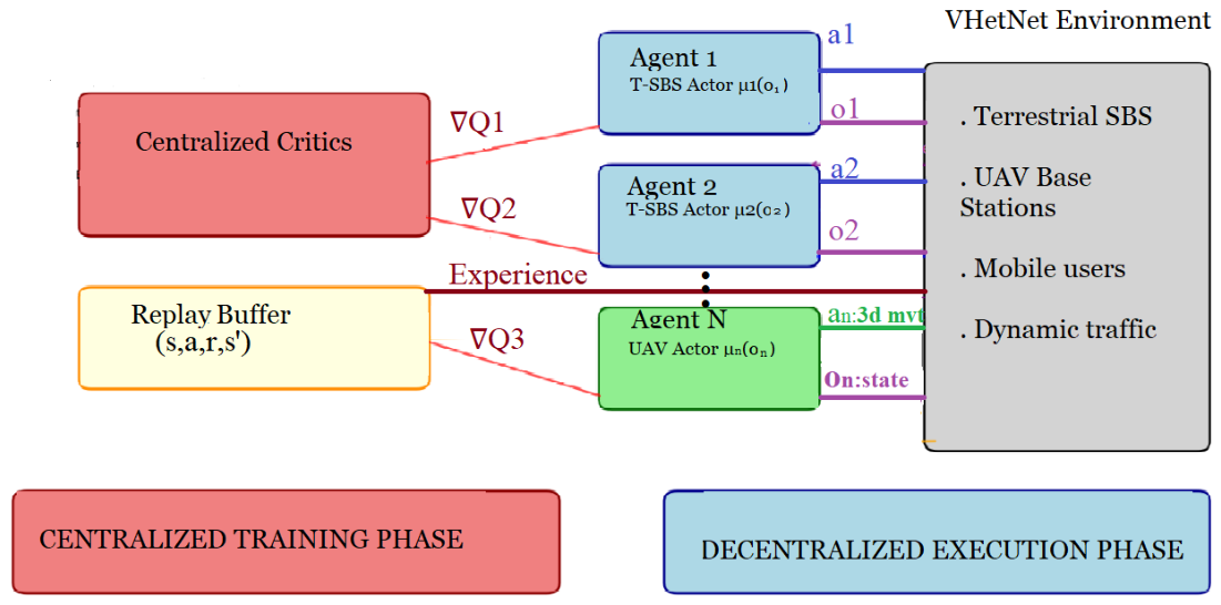
Figure 2.
System Model: Dynamic UAV Assisted HetNet with Task distribution.
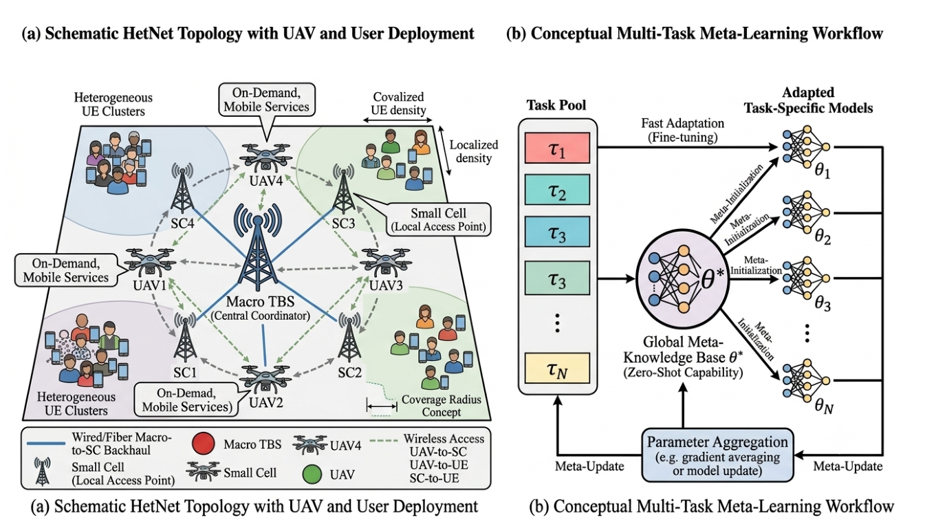
Figure 3.
Performance degradation of MARL-ESA when deployed on unseen topologies, highlighting the need for generalization.
Figure 3.
Performance degradation of MARL-ESA when deployed on unseen topologies, highlighting the need for generalization.
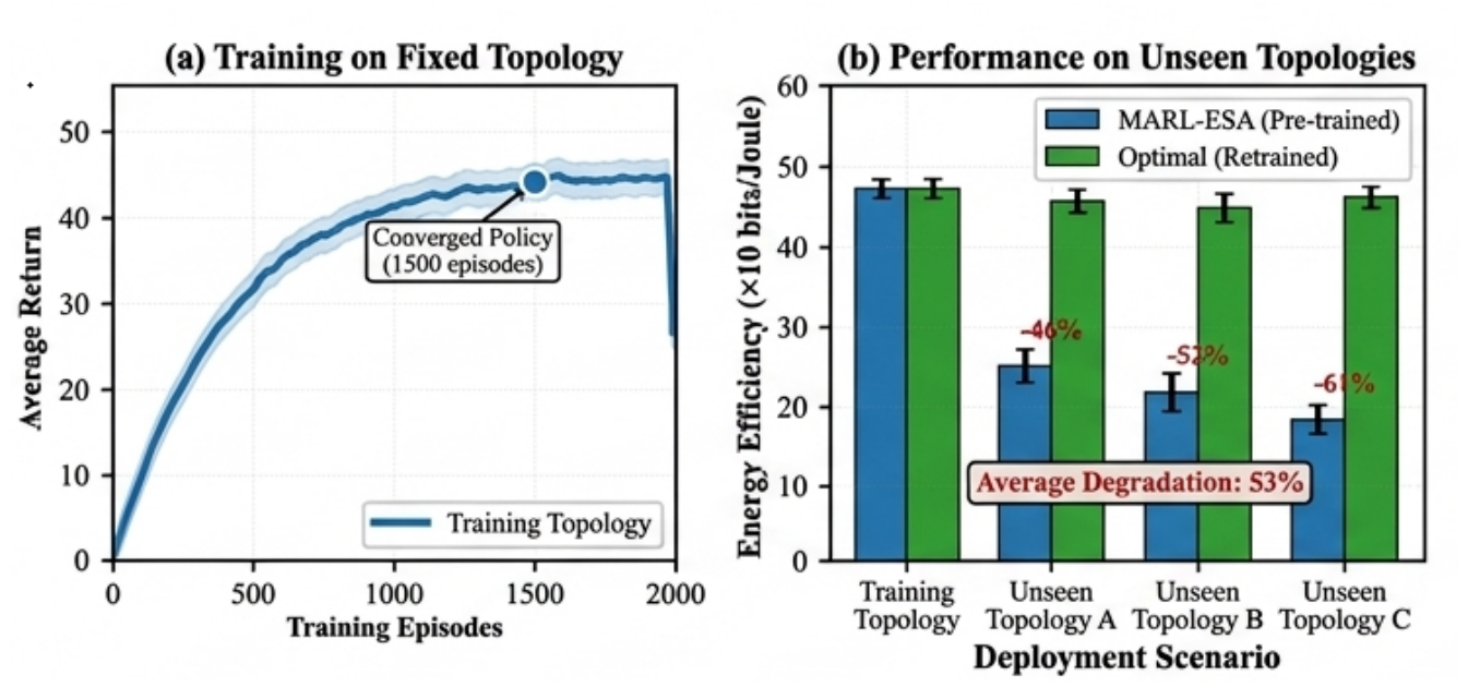
Figure 4.
GNN architecture.
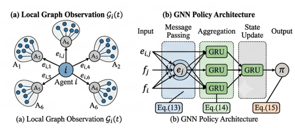
Figure 5.
Energy consumption breakdown showing 48% total energy savings (2150 W to 1110 W) compared with always-on operation.
Figure 5.
Energy consumption breakdown showing 48% total energy savings (2150 W to 1110 W) compared with always-on operation.
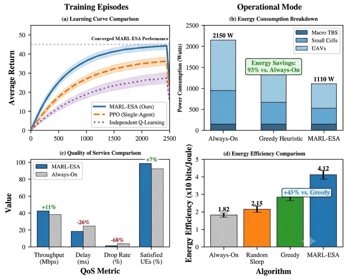
Figure 6.
Convergence rate comparison on an unseen task. Meta-MARL-ESA shows superior jumpstart performance and converges approximately 12× faster than training from scratch.
Figure 6.
Convergence rate comparison on an unseen task. Meta-MARL-ESA shows superior jumpstart performance and converges approximately 12× faster than training from scratch.
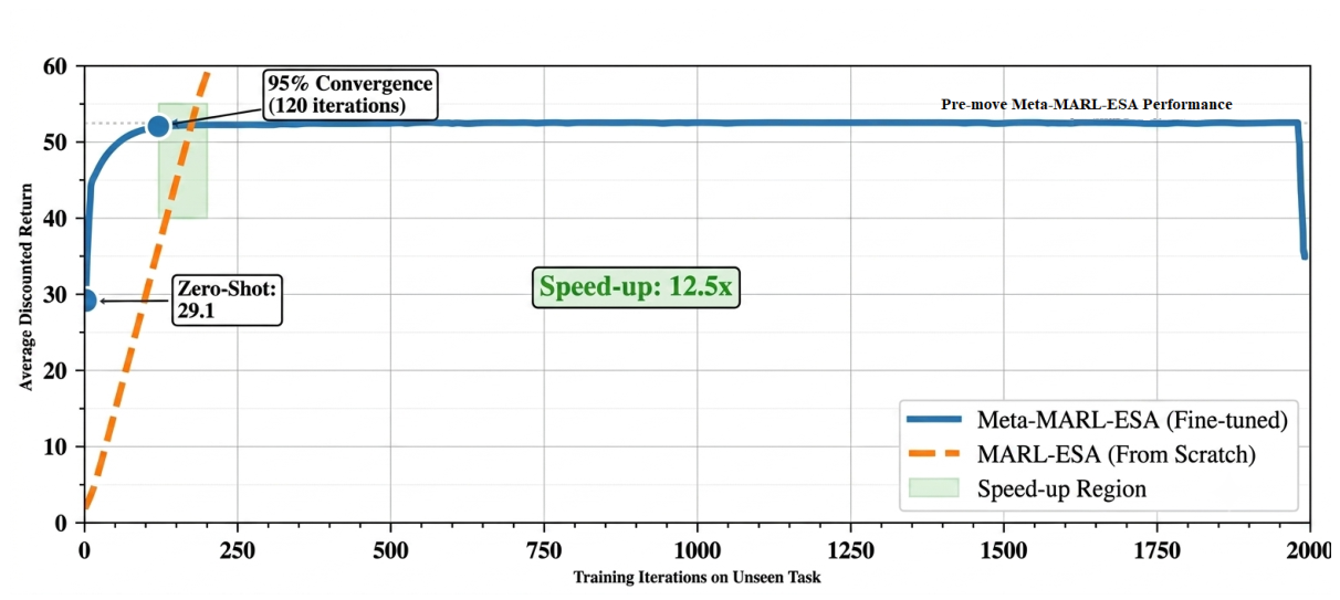
Figure 7.
Energy efficiency vs. spectral efficiency trade-off curve on . The solid markers indicate non-dominated operating points (points for which no other point achieves both higher EE and higher SE), while the dashed lines represent quadratic fits to the empirical data.
Figure 7.
Energy efficiency vs. spectral efficiency trade-off curve on . The solid markers indicate non-dominated operating points (points for which no other point achieves both higher EE and higher SE), while the dashed lines represent quadratic fits to the empirical data.
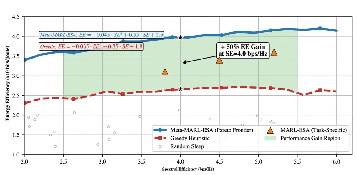
Figure 8.
Adaptation to sudden UAV repositioning at s. Meta-MARL-ESA recovers optimal performance within 5-8 decision epochs.
Figure 8.
Adaptation to sudden UAV repositioning at s. Meta-MARL-ESA recovers optimal performance within 5-8 decision epochs.
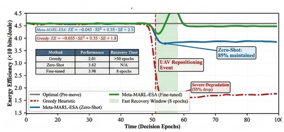

Table 1.
Comparative Analysis of Existing Work.
| Reference | Approach | Network Type | Generalization | Limitations |
|---|---|---|---|---|
| [6] | Heuristic Threshold | Terrestrial HetNet | None | Rule-based, cannot adapt to traffic |
| [7] | Independent Q-Learning | Small Cell Networks | None | Non-stationarity, poor convergence |
| [8] | MADDPG | UAV-Assisted HetNet | None | Fixed topology, retraining required |
| [9] | GNN + RL | Ad hoc Networks | Limited | Size generalization only |
| [10] | DDQN + Meta-RL | Vehicular Networks | Moderate | Single-agent only |
| [11] | Iterative Optimization (SCA) | Multi-UAV IoT | None | Requires full CSI, no learning-based adaptation |
| [12] | Joint Optimization (Iterative) | SAGIN | None | Non-convex, high complexity, static optimization |
| [13] | MARL (Trajectory + Handover) | UAV-Assisted 6G HetNets | Limited | No meta-learning, requires retraining for new topologies |
| [14] | MARL + PPO (GLIDE) | UAV Fleet Control | Limited | Focuses on task completion time, not sleep scheduling |
| [15] | Multi-Agent DRL | Cognitive UAV-MEC HetNets | Limited | Focuses on energy efficiency in MEC, not sleep scheduling |
| Proposed Frameworks | ||||
| MARL-ESA | CTDE MARL | UAV-Assisted HetNet | None | Static topology baseline |
| Meta-MARL-ESA | GNN + MAML | Dynamic 6G NTN | Zero-Shot + Rapid | Addresses the limitations identified in existing works |
Table 2.
List of Abbreviations.
| Abbreviation | Full Form |
|---|---|
| 3GPP | 3rd Generation Partnership Project |
| 5G/B5G | Fifth / Beyond Fifth Generation |
| 6G | Sixth Generation |
| HetNet | Heterogeneous Network |
| NTN | Non-Terrestrial Network |
| UAV | Unmanned Aerial Vehicle |
| UABS | UAV-Mounted Aerial Base Station |
| TBS | Terrestrial Base Station |
| UE | User Equipment |
| QoS | Quality of Service |
| LoS/NLoS | Line / Non-Line of Sight |
| EE | Energy Efficiency |
| SE | Spectral Efficiency |
| RL | Reinforcement Learning |
| MARL | Multi-Agent RL |
| Meta RL | Meta-Reinforcement Learning |
| MAML | Model-Agnostic Meta-Learning |
| GNN | Graph Neural Network |
| MPNN | Message Passing Neural Network |
| MLP | Multi-Layer Perceptron |
| CTDE | Centralized Training / Decentralized Execution |
| PPO | Proximal Policy Optimization |
| MADDPG | Multi-Agent Deep Deterministic Policy Gradient |
| Dec-POMDP | Decentralized Partially Observable MDP |
| MDP | Markov Decision Process |
| GRU | Gated Recurrent Unit |
Table 3.
Node-Type Differentiated Power Parameters and Consumption Breakdown.
| Node Type | (W) | (W) | (W) | Max Savings (W) | |
|---|---|---|---|---|---|
| Macro TBS | 150 | 200 | 4.7 | 0 | 50 |
| Small Cell TBS | 50 | 200 | 3.2 | 0 | 150 |
| UAV | 50 | 80 | 2.1 | 300 / 50 | 250 |
Table 4.
Hyperparameters Used in Meta-MARL-ESA and Baseline Training.
| Parameter | Value |
|---|---|
| GNN hidden dimension | 128 |
| Number of GNN layers | 3 |
| GRU hidden dimension | 128 |
| PPO clipping parameter | 0.2 |
| Actor learning rate | |
| Critic learning rate | |
| Inner-loop learning rate | 0.01 |
| Meta-learning rate | 0.001 |
| Number of inner-loop steps K | 1 |
| Meta-batch size | 8 |
| Number of training tasks | 5000 |
| Episode length | 100 steps |
| Discount factor | 0.95 |
| GAE parameter | 0.95 |
| Random seeds | 42, 43, 44, 45 |
Table 5.
Key Simulation Parameters.
| Parameter | Value |
|---|---|
| Network Area | 2 km × 2 km urban grid |
| Macro TBS () | 1, fixed at center, height 30 m |
| Small Cell TBSs | , height 10 m |
| UABSs | , altitude 100–150 m |
| UE Clusters | 50, uniformly distributed |
| Carrier Frequency () | 2 GHz |
| Bandwidth (W) | 20 MHz |
| UAV Mass () | 2 kg |
| UAV Hover Power | 300 W |
| TBS Power Parameters | W, |
| W, | |
| –10 W [30] | |
| Reward Weights () | , , |
| Discount Factor () | 0.95 |
| Slope Factor () | 4.7 |
| Amplifier Efficiency () | 0.38 |
Table 6.
Average Energy Efficiency ( bits/Joule) Across Task Distributions.
| Algorithm | |||
|---|---|---|---|
| Random | 1.21 | 1.19 | 0.98 |
| Greedy Heuristic | 2.85 | 2.81 | 2.05 |
| MARL-ESA (from scratch, converged) | 4.12 | 3.95 | 2.89 |
| Meta-MARL-ESA (Zero-Shot) | 3.88 | 3.82 | 3.51 |
| Meta-MARL-ESA (Fine-Tuned) | – | 4.05 | 3.92 |
Table 7.
Ablation Study: Zero-Shot EE on ( bits/Joule).
| Configuration | Zero-Shot EE |
|---|---|
| MARL + MLP | 2.15 |
| MARL + GNN (no meta) | 2.98 |
| MAML + MLP | 2.87 |
| Meta-MARL-ESA (GNN + MAML) | 3.51 |
Disclaimer/Publisher’s Note: The statements, opinions and data contained in all publications are solely those of the individual author(s) and contributor(s) and not of MDPI and/or the editor(s). MDPI and/or the editor(s) disclaim responsibility for any injury to people or property resulting from any ideas, methods, instructions or products referred to in the content. |
© 2026 by the authors. Licensee MDPI, Basel, Switzerland. This article is an open access article distributed under the terms and conditions of the Creative Commons Attribution (CC BY) license (http://creativecommons.org/licenses/by/4.0/).
Copyright: This open access article is published under a Creative Commons CC BY 4.0 license, which permit the free download, distribution, and reuse, provided that the author and preprint are cited in any reuse.