

Submitted:
01 October 2026
Posted:
05 October 2026
You are already at the latest version
Abstract
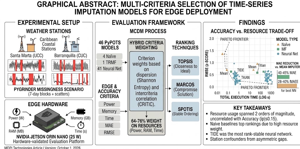
Reconstructing missing values in meteorological time series is essential for reliable renewable-energy assessment, but on-device imputation must respect the power, memory and latency budget of edge hardware. We benchmark 46 PyPOTS imputation models—four naïve baselines, TRMF and 41 neural networks—on two tropical coastal stations (UCC and CUC, Colombian Caribbean) resampled to 15 min and subjected to a PyGrinder missingness scenario, running each model on an NVIDIA Jetson Orin Nano (25 W) and measuring MAE, RMSE, power, memory and time. A hybrid Entropy–CRITIC weighting scheme with TOPSIS and MARCOS ranked the alternatives. The best neural networks cut the mean-imputer error by 40–45% (MAE) and 28–40% (RMSE), yet resource usage spanned two orders of magnitude, uncorrelated with accuracy (|ρ|≤0.15). Because both methods placed 64–76% of the weight on resource criteria, naïve baselines and TRMF topped the station-averaged and UCC rankings, TiDE was the most rank-stable neural network, and SCINet led at CUC under the untuned configuration. TOPSIS and SPOTIS agreed closely (ρ≥0.98); MARCOS agreed moderately with both (ρ≈0.68–0.93). Station-to-station agreement was low for TOPSIS (ρ=0.52)—a confound rather than a station effect: the same masking configuration produced an asymmetric gap structure at the shorter, previously incomplete UCC record and a uniform one at the longer, complete CUC record, so station-level conclusions are not directly comparable. An automated per-model hyperparameter-search protocol, which reorders the CUC top, is provided in an appendix. These results offer a reproducible, hardware-validated framework for edge-constrained imputation model selection.
Keywords:
time-series imputation
; missing data
; edge computing
; NVIDIA Jetson Orin Nano
; multicriteria decision-making
; Shannon entropy
; CRITIC
; TOPSIS
; MARCOS
; SPOTIS
; PyPOTS
; hyperparameter optimization
; renewable energy
; tropical meteorology
1. Introduction
The availability, quality, and traceability of meteorological data are fundamental for various initiatives related to renewable energy, agriculture, environmental modeling, and climate risk management [1,2]. In particular, assessing the feasibility and performance of wind power generation projects requires reliable meteorological information that is representative of local microclimatic conditions, including variables such as wind speed and direction, atmospheric pressure, and temperature [3,4,5,6]. However, in situ records often exhibit data gaps resulting from instrumentation failures, transmission disruptions, maintenance deficiencies, or equipment degradation caused by exposure to harsh environmental conditions [7,8]. These discontinuities compromise time-series integrity, reduce the accuracy of predictive models, and negatively impact strategic decision-making [9,10].
In the presence of missing data, the use of satellite or reanalysis sources represents a common alternative due to their broad spatial coverage [11,12]. Nevertheless, their limited spatial and temporal resolution hinders the capture of zonal atmospheric dynamics and specific microclimatic patterns [13]. This limitation is particularly critical in tropical coastal regions—such as the Colombian Caribbean Coast [14,15,16]—where low monitoring network density, combined with bias and intermittency in observations, introduces substantial operational and financial uncertainties in energy planning [17,18]. In this context, time-series reconstruction using quality control schemes and data imputation becomes indispensable to ensure high-fidelity meteorological estimates [19,20].
In recent literature, time-series imputation strategies are primarily categorized into three groups: traditional statistical methods, Machine Learning (ML) techniques, and Deep Learning (DL) approaches [21,22]. While statistical methods stand out for their low computational cost, they demonstrate limited performance when handling non-linear dependencies [23,24]. Conversely, ML and DL architectures effectively capture complex temporal patterns and multivariate dependencies at the expense of higher demand for memory and computational resources [25,26]. Nevertheless, evidence indicates that no single algorithm is universally superior; performance varies depending on the loss mechanism, the length of missing data intervals, and the deployment environment constraints [27,28].
In Edge Computing environments, selecting an imputation model depends not only on statistical accuracy but also on a critical trade-off with hardware-constrained resources such as latency, energy consumption, and RAM footprint [27]. To address complex decision problems involving alternatives with conflicting criteria, numerous studies have demonstrated the effectiveness of Multi-Criteria Decision-Making (MCDM) frameworks by combining objective weightings and ranking techniques [29,30]. Despite these advancements, two main gaps persist in the literature: i) the lack of a systematic evaluation of the behavior of imputation models under long contiguous data gaps in tropical climate conditions, and ii) the absence of a holistic decision framework that simultaneously evaluates the statistical fidelity of the reconstruction and the physical hardware constraints on peripheral processing nodes.
To overcome these limitations, this paper presents an experimental study focused on the holistic evaluation of time-series imputation models for meteorological data from the Colombian Caribbean region, specifically in the cities of Santa Marta and Barranquilla, deployed on Edge Computing hardware—namely, the NVIDIA Jetson Orin Nano. In this context, the main contribution of this paper lies in implementing an integrated Multi-Criteria Decision-Making (MCDM) methodological framework. This framework combines a hybrid criteria weighting approach using two fully objective, data-driven methods—the Shannon Entropy method and the Criteria Importance Through Intercriteria Correlation (CRITIC) method—with a parallel ranking of imputation algorithms via the Technique for Order Preference by Similarity to Ideal Solution (TOPSIS) and Measurement of Alternatives and Ranking according to Compromise Solution (MARCOS) techniques. Using two fully objective weighting methods keeps the whole weighting stage reproducible directly from the measured decision matrix, without any subjective human elicitation step. Furthermore, the stability of the resulting ranking is validated using the Stable Preference Ordering Towards Ideal Solution (SPOTIS) method and Spearman’s rank correlation coefficient. A secondary contribution is a fully automated, per-model hyperparameter-search protocol, provided as a self-contained script suite in Appendix C, which the practitioner can run on the same edge hardware to replace the common compact configuration used for the main benchmark with a tuned one. Through this approach, the performance of traditional, Machine Learning (ML), and Deep Learning (DL) architectures is holistically evaluated, balancing statistical reconstruction accuracy, Root Mean Square Error (RMSE), Mean Absolute Error (MAE) with real-time operational hardware metrics such as energy consumption, inference latency, and RAM occupancy on the Edge architecture.
Additionally, the robustness of the resulting ranking is analyzed with respect to the weighting coefficient, the ranking algorithm and the monitoring station, under a demanding missingness scenario that combines randomly scattered gaps with long contiguous gaps in key wind and thermodynamic variables for tropical coastal areas. As a result, this study provides a reproducible and directly transferable methodological guide for the optimization and deployment of data quality control and imputation models in advanced distributed environmental monitoring networks.
2. Materials and Methods
2.1. Monitoring Stations
The weather stations are located at Universidad de la Costa and Universidad Cooperativa de Colombia, as shown in Figure 1, whereas Figure 2 presents photographs of the physical installations.
Regarding the deployment sites of the meteorological stations, both site characteristics and data acquisition frequencies were carefully evaluated, as these conditions directly affect the representativeness of the recorded atmospheric variables. The monitoring station at Universidad de la Costa (CUC) in Barranquilla (located at an altitude of 24 m a.s.l.) is installed on the rooftop of the Laboratory Building (Block 12), placing its sensors at a height of approximately 28 to 32 m above ground level. This station acquired meteorological data at a sampling rate of 15 minutes during the first two months of operation, and 5 minutes for the remaining period.
In contrast, the weather station at the Santa Marta Campus of Universidad Cooperativa de Colombia (UCC), situated at an altitude of 28 m a.s.l. in Santa Marta, is installed at ground level in proximity to student activity facilities (specifically adjacent to the multipurpose sports court). Unlike the rooftop setup at CUC, this configuration enables atmospheric measurements under conditions closer to those directly experienced in the campus surface environment. The UCC station natively acquires data at 5 minutes per record, providing higher temporal resolution to analyze local microclimatic variability; for this study it was resampled to the common 15-min grid described below.
To standardize data processing across both monitoring sites, both records were placed on the same regular 15-min time grid (2049 records at UCC, spanning 21.3 days; 6251 records at CUC, spanning 65.1 days) before the PyGrinder missingness scenario of Section 3.1 was generated. Consequently, a given number of samples corresponds to the same time span at both stations throughout this paper (e.g., the 96-sample imputation window used in Section 2.5 spans 24 h at both stations). The technical specifications of the weather stations are detailed in Table 1.
2.1.1. Raw Dataset
Table 2 presents the start and end dates of the data recording period for this study, while Table 3 provides the summary statistics.
Where:
- Avg. Wind Speed: represents the average wind speed.
- Avg. Wind Direction: represents the average wind direction.
- Rel. Humidity: represents the relative humidity.
- Air Temp.: represents the air temperature.
To avoid numerical boundary discontinuities at the angular limit () during the training of the imputation models, average wind speed (V, Avg. Wind Speed) and average wind direction (, Avg. Wind Direction) were transformed into continuous Cartesian components ( and ) using Equations (1) and (2):
Where:
- : represents the x-axis Cartesian component derived from the sinusoidal projection of the wind vector.
- : represents the y-axis Cartesian component derived from the cosinusoidal projection of the wind vector.
- V: represents the magnitude of the wind vector (Avg. Wind Speed).
- : represents the wind direction in degrees (Avg. Wind Direction).
Additionally, to capture the temporal cyclicity of the observations without introducing artificial discontinuities at period boundaries, cyclic features were created for the hour of the day (hour) and the day of the year (doy) using Equations (3)–(6):
- : represents the normalized variable.
- x: represents the original raw data value.
- : represents the sample mean of x.
- : represents the sample standard deviation of x.
2.2. Clean Dataset
To perform the study, continuous time segments with the lowest proportion of missing observations were selected from both the CUC and UCC station datasets, corresponding to the date ranges specified in Table 4.
Figure 3 depicts the wind roses generated from raw wind speed and direction data recorded at each station, illustrating the directional distribution and relative frequency of wind occurrences across angular sectors. This representation characterizes the dominant wind resource at each deployment site and serves as a useful benchmark to guide decision-making regarding the placement and orientation of wind turbines or other sensors sensitive to airflow direction.
The statistical summary of the normalized data is provided in Table A1. Figure 4 illustrates the clean dataset for the CUC station, which contains no missing values. Conversely, Figure 5 shows the UCC station dataset, which exhibits missing records, specifically in Humidity (), Air Temp. (), and Windcos and Windsin ( each). Because this pre-existing incompleteness was carried forward into the artificial masking step described in Section 3.1, it is a contributing factor—together with the shorter length of the UCC record—to the asymmetric missingness scenario ultimately realized at that station.
2.3. Models
For experimental evaluation, a diverse set of 46 imputation models was selected from the open-source PyPOTS ecosystem (Python Toolkit for Machine Learning on Partially-Observed Time Series) [31]. As detailed in Figure 6 and Table A2, the selected models range from basic baseline methods to advanced deep learning architectures, categorized into three primary groups:
- Naïve Models (4 models): Deterministic methods and low-computational-cost simple statistical interpolations (linear interpolation, mean, median, and Last Observation Carried Forward / Next Observation Carried Backward), used as baseline benchmarks for comparison.
- Matrix Factorization (MF - 1 model): Represented by TRMF (Temporal Regularized Matrix Factorization), which leverages low-rank autoregressive structures in time series.
- Deep Neural Networks (Neural Networks - 41 models): A broad array of Deep Learning architectures encompassing recurrent models (GRU-D, BRITS), convolutional and frequency-domain models (TCN, TimesNet, ModernTCN), graph-based architectures and probabilistic autoencoders (StemGNN, GP-VAE, CSDI), as well as the latest Transformer variants tailored for time series (SAITS, iTransformer, PatchTST, ImputeFormer, Autoformer).
2.4. Edge Evaluation Hardware Platform: NVIDIA Jetson Orin Nano
The experimental deployment and real-time hardware performance characterization were conducted on an NVIDIA Jetson Orin Nano (Super reference developer kit). From an engineering and operational perspective, edge processing hardware system are particularly vital in developing regions, where structural constraints such as bandwidth limitations, unstable power grids, and restricted hardware budgets hinder cloud-dependent processing frameworks. By performing localized data quality control and imputation, edge architectures eliminate continuous cloud bandwidth dependencies, lower operational overhead, and safeguard against data loss during connectivity outages.
Equipped with 1024 NVIDIA Ampere architecture Compute Unified Device Architecture (CUDA) cores—specialized parallel processing units that accelerate general-purpose matrix operations—and 32 dedicated Tensor Cores, the Jetson Orin Nano provides localized compute capability. It delivers up to 67 Trillion Operations Per Second (TOPS), a metric quantifying the raw AI throughput capability of the board for integer and floating-point inferences, within a thermal design power (TDP) envelope adjustable between 7 W and 25 W across its three predefined power modes. This power footprint enables sustained, off-grid field operation powered by localized solar-battery configurations or auxiliary power supplies. Furthermore, its unified 8 GB Low Power Double Data Rate 5 (LPDDR5) memory architecture—a high-bandwidth, energy-efficient DRAM technology optimized for mobile and embedded systems—facilitates the low-latency execution of complex multivariate deep learning imputation models without the memory bandwidth bottlenecks typical of traditional edge hardware.
The detailed technical specifications of the hardware platform and the deployed software stack are summarized in Table 5. All experiments were run in the highest-performance 25 W power mode of the board (nvpmodel reported “NV Power Mode: 25W” on the host at the time of the experiments); the on-board INA3221 power monitor was used to measure power directly rather than assuming the value of the selected mode.
2.5. Imputation Experiments and Measurement Protocol
The evaluation followed a transductive gap-filling protocol: each model was fitted on the incomplete series of a station (natural gaps plus the gaps injected with PyGrinder, see Section 3.1) and then used to impute that same series. The ground truth of the masked cells was therefore never exposed to any model, and no separate validation or test partition was used, which reflects the operational task of reconstructing the gaps of a recorded series. Accuracy was quantified exclusively on the set of cells masked by PyGrinder, pooling the four target variables and excluding the naturally missing cells, whose true value is unknown:
where and are the true (standardized) and imputed values of variable v at time t. Errors are therefore expressed in z-score units.
The series were segmented into windows of consecutive samples, corresponding to 24 h at both stations once both records were placed on the common 15-min grid. Training used overlapping windows with a stride of 24 samples, and imputation used non-overlapping windows covering the whole series (the last window was padded with missing values). The 41 neural networks were trained for 50 epochs with a batch size of 32, without early stopping and with a fixed pseudorandom seed of 42. To keep the resource comparison independent of unequal tuning effort, a common compact configuration was used wherever the architecture allows it (two layers, hidden size 64 and four attention heads), and hyperparameters were not tuned individually. The four naïve methods were applied to the complete series as a single sample, TRMF was fitted on the CPU, and the neural networks were executed on the GPU. Experiments used PyPOTS 1.5 and PyTorch 2.2.0 on the platform of Table 5.
Each model was executed in an isolated process so that memory peaks could be attributed to individual models. The three edge criteria were measured as follows: (i) Power is the average board power during fitting and inference (weighted by phase duration), obtained by sampling the on-board INA3221 power monitor every 20 ms; each measured phase was extended, after an unmeasured warm-up call, to cover at least 3 s so that the number of power samples per phase would not depend on the raw speed of the call (median of 1222 samples for fitting and 108 for inference across the 92 runs); the idle power of the board, measured over 20 s before the experiments, was 5.08 W. (ii) RAM is the peak resident memory of the process plus the GPU memory reserved by PyTorch, which is the relevant figure on a device with unified memory; and (iii) Time is the fitting time plus the latency of one full-series imputation call. Because training dominates this criterion, it represents the cost of fitting and using a model directly on the device. In addition to the decision matrices of each station, a station-averaged decision matrix was built by averaging each criterion over the two stations, in order to obtain a single ranking of the 46 alternatives.
2.6. Multi-Criteria Decision-Making Tools
The evaluation, ranking, and selection of the highest-ranked imputation model among the candidate alternatives on embedded hardware was formulated as a Multi-Criteria Decision Analysis (MCDA) problem. Numerical processing and decision model resolution were executed in R software (version 4.1.2) [32] utilizing the RMCDA package (version 0.3.1) [33].
To structure the decision matrix, a set of criteria was considered, split into two key dimensions: imputation accuracy and computational efficiency on the edge device, as detailed in Table 6.
2.6.1. Hybrid Criteria Weighting: Entropy and CRITIC
Eliciting criteria weights from a human expert introduces a subjective element that is difficult to reproduce or audit, and that must be re-elicited whenever the criteria set or the application domain changes. To keep the whole weighting stage fully objective and reproducible directly from the measured decision matrix, this study instead combines two data-driven weighting methods, the Shannon Entropy method and CRITIC, so that both components of the hybrid scheme are computed solely from the observed decision matrix, without any human elicitation step.
Objective Weighting via Shannon Entropy:
The Entropy method [34,35] quantifies the discriminating power of a criterion from the dispersion of its values across alternatives: a criterion whose observed values are very similar across the alternatives carries little information for distinguishing between them and receives a low weight, whereas a criterion with a highly uneven distribution of values receives a high weight. To make the Entropy weights comparable across criteria measured in different units and to avoid a criterion with a much wider numerical range (in this study, the training-plus-inference time, which spans more than three orders of magnitude) dominating the weight purely because of its scale, Entropy was computed on the same cost-oriented min–max normalized matrix of Equation (12) used by CRITIC and TOPSIS, rather than on the raw decision matrix. Each column of was first turned into a probability distribution over the m alternatives,
and the entropy and degree of diversification of criterion j were then obtained as
with the usual convention when , which occurs for the best and the worst alternative of every criterion because for those rows. The objective weights are obtained by normalizing the diversification degrees:
Objective Weighting via CRITIC:
Complementarily, objective weights were derived directly from the decision matrix using the Criteria Importance Through Intercriteria Correlation (CRITIC) algorithm [36]. Since all criteria in Table 6 represent cost metrics (where lower values denote superior performance), the matrix was normalized via min-max transformation:
The amount of information contained in the j-th criterion is quantified by combining the intrinsic dispersion of its measurements, expressed by its standard deviation , with the informational conflict relative to other metrics, derived from the Pearson correlation matrix :
The objective weights are obtained by normalizing the values:
Hybrid Weight Integration:
The final criteria weights were calculated using a balanced linear combination of the Entropy and CRITIC weight vectors, ensuring that :
where is the trade-off weighting coefficient between the two objective weighting schemes ( in the base case). Because both and are derived only from the observed decision matrix, blends two complementary, purely objective measures of the same data structure—dispersion relative to a common scale (Entropy) and dispersion combined with cross-criteria redundancy (CRITIC)—and its sensitivity is examined in Section 3.6.
2.6.2. Ranking Algorithms: TOPSIS and MARCOS
The hierarchical ranking of the imputation alternatives was executed in a parallel and comparative manner using the TOPSIS and MARCOS methods.
TOPSIS Method:
The Technique for Order Preference by Similarity to Ideal Solution (TOPSIS) algorithm [37] identifies the best alternative based on the shortest Euclidean distance to the Positive Ideal Solution () and the farthest distance from the Negative Ideal Solution (). From the weighted normalized decision matrix (where , and is the cost-oriented min–max normalization of Equation (12), so that TOPSIS and CRITIC share the same normalized matrix), the ideal points are defined as and .
The Euclidean distances and for each model i are expressed as:
The relative closeness coefficient determines the final descending rank ():
MARCOS Method:
The Measurement of Alternatives and Ranking according to Compromise Solution (MARCOS) algorithm [38] evaluates compromise solutions relative to ideal () and anti-ideal () reference points, which are explicitly included as additional rows of the extended decision matrix. For cost criteria, and . The extended matrix was normalized with the ratio-based transformation
so that MARCOS uses the raw (positive) values of the criteria and a normalization different from the range-based one of CRITIC and TOPSIS. For each model i, the weighted sum of its normalized values, , is used to compute utility degrees with respect to the anti-ideal and ideal solutions:
where and are the weighted sums of the and rows, respectively. From these degrees, the utility functions of each model relative to the ideal and anti-ideal solutions are defined as:
Finally, the aggregated utility function , which synthesizes both compromises into a unified performance index, is defined as:
Alternatives are ranked in descending order according to , with the highest value indicating the compromise solution closest to ideal. Because ratio-based and range-based normalizations weigh differently the differences among alternatives when a criterion spans several orders of magnitude, differences between the TOPSIS and MARCOS rankings are expected and are analyzed in Section 3.6.
2.6.3. Sensitivity Analysis and Ranking Robustness
To verify that the resulting ranking is not a mathematical artifact of the specific distance metrics and normalizations employed by TOPSIS and MARCOS, an inter-algorithmic cross-validation was conducted against the Stable Preference Ordering Towards Ideal Solution (SPOTIS) method [39]. For cost criteria, SPOTIS measures the normalized distance of each alternative to the ideal point within the criterion bounds and aggregates it with the criteria weights (lower scores are better):
SPOTIS is free of rank reversal when the bounds are fixed a priori by the decision maker, independently of the set of alternatives. In this study the bounds were set to the minimum and maximum observed values of each criterion, so this invariance was not exploited and SPOTIS was used as a consistency check based on a normalization different from that of MARCOS, not as a rank-reversal-free reference.
The mathematical concordance between the rankings generated by TOPSIS, MARCOS, and SPOTIS was quantitatively evaluated using Spearman’s rank correlation coefficient ():
where represents the difference between the ranks assigned to alternative i by two distinct methodologies (ties were handled by assigning average ranks, i.e., is computed as the Pearson correlation of the ranks). A value of indicates convergence between the methods. Three additional robustness analyses were performed: (i) the coefficient of Equation (15) was varied over , and both the Spearman correlation of each resulting ranking with the baseline ranking () and the identity of the best-ranked model were recorded; (ii) the Spearman correlation between the rankings obtained at the two stations was computed for each method; and (iii) the analyses were repeated for the station-specific and the station-averaged decision matrices.
3. Results
3.1. Experimental Evaluation Setup
To generate the test dataset, PyGrinder from the PyPOTS ecosystem was utilized. Both stations were first placed on a common, regular 15-min grid (2049 records at UCC, 21.3 days; 6251 records at CUC, 65.1 days), so that a given number of samples corresponds to the same time span at both stations, and missing values were then introduced independently for each target variable, as detailed in Table 8 below.
The missingness scenario actually realized by PyGrinder is characterized in Table 8. At CUC, every target variable received the intended combination of randomly scattered missing values plus one contiguous block of 672 consecutive missing samples (7 days); 84–87% of the masked cells of each variable belong to that block. At UCC, only relative humidity and Windsin received a comparable block (also 672 samples, 7 days, i.e. a third of the 21.3-day record), while air temperature and received only the randomly scattered component, with no contiguous block: their masked cells are isolated or span at most two consecutive samples. The UCC series additionally contains 57 naturally missing cells (12, 19, 13 and 13 in temperature, humidity, and , respectively) that were excluded from all accuracy computations because their true value is unknown; the CUC series has no natural gaps. This difference in the starting condition of the two series, combined with the shorter UCC record (2049 versus 6251 samples), is the most plausible explanation for why the same PyGrinder configuration landed the 7-day contiguous block on only two of the four UCC variables, whereas at CUC—longer and free of natural gaps before masking—every variable received one: with fewer eligible starting positions on a shorter, partially pre-masked series, the stochastic block-placement step is more likely to miss some variables entirely, an outcome discussed further in Section 4.3. Note that the two UCC variables with a block (humidity, 696 masked cells; , 686) do not equal the naive sum of the 672-sample block plus a full independent scatter (): the scattered component is drawn independently over the whole 2049-sample series, so roughly a third of those draws () fall inside the block window itself or on one of the station’s pre-existing natural gaps and reveal no additional cell, leaving a net scattered contribution of only 24 and 14 cells, respectively (696−672 and 686−672); the two UCC variables without a block (air temperature, ) are not subject to this overlap and their counts (31 and 41) are correspondingly closer to the nominal of 2049. All 46 models were fitted and evaluated at both stations following the protocol of Section 2.5: the 92 runs completed without failures, and the cumulative fitting-plus-inference time was 2.53 h (1.90 h at CUC, 0.63 h at UCC).

Table 7.
Statistical summary of the test dataset (PyGrinder-masked series) for both stations, on the common 15-min grid.
Table 7.
Statistical summary of the test dataset (PyGrinder-masked series) for both stations, on the common 15-min grid.
| Station | Variable | N | Valid (n) | Min | Q1 | Median | Mean | Q3 | Max | Missing (n) | Missing (%) |
|---|---|---|---|---|---|---|---|---|---|---|---|
| CUC | Rel. Humidity | 6251 | 5474 | 777 | |||||||
| Air Temp. | 6251 | 5465 | 786 | ||||||||
| 6251 | 5455 | 796 | |||||||||
| 6251 | 5482 | 769 | |||||||||
| UCC | Rel. Humidity | 2049 | 1334 | 715 | |||||||
| Air Temp. | 2049 | 2006 | 43 | ||||||||
| 2049 | 1995 | 54 | |||||||||
| 2049 | 1350 | 699 |
Figure 7.
Test variables for the CUC station.
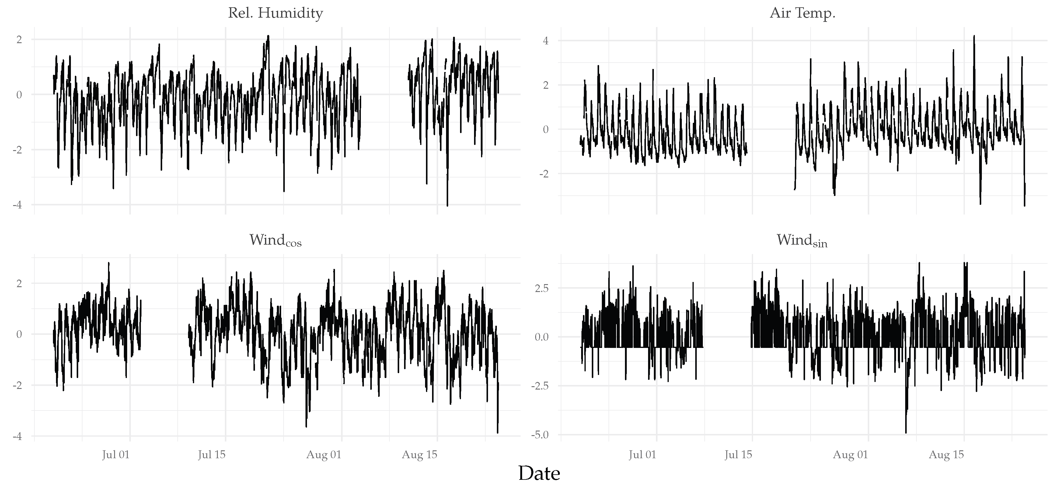
Figure 8.
Test variables for the UCC station.
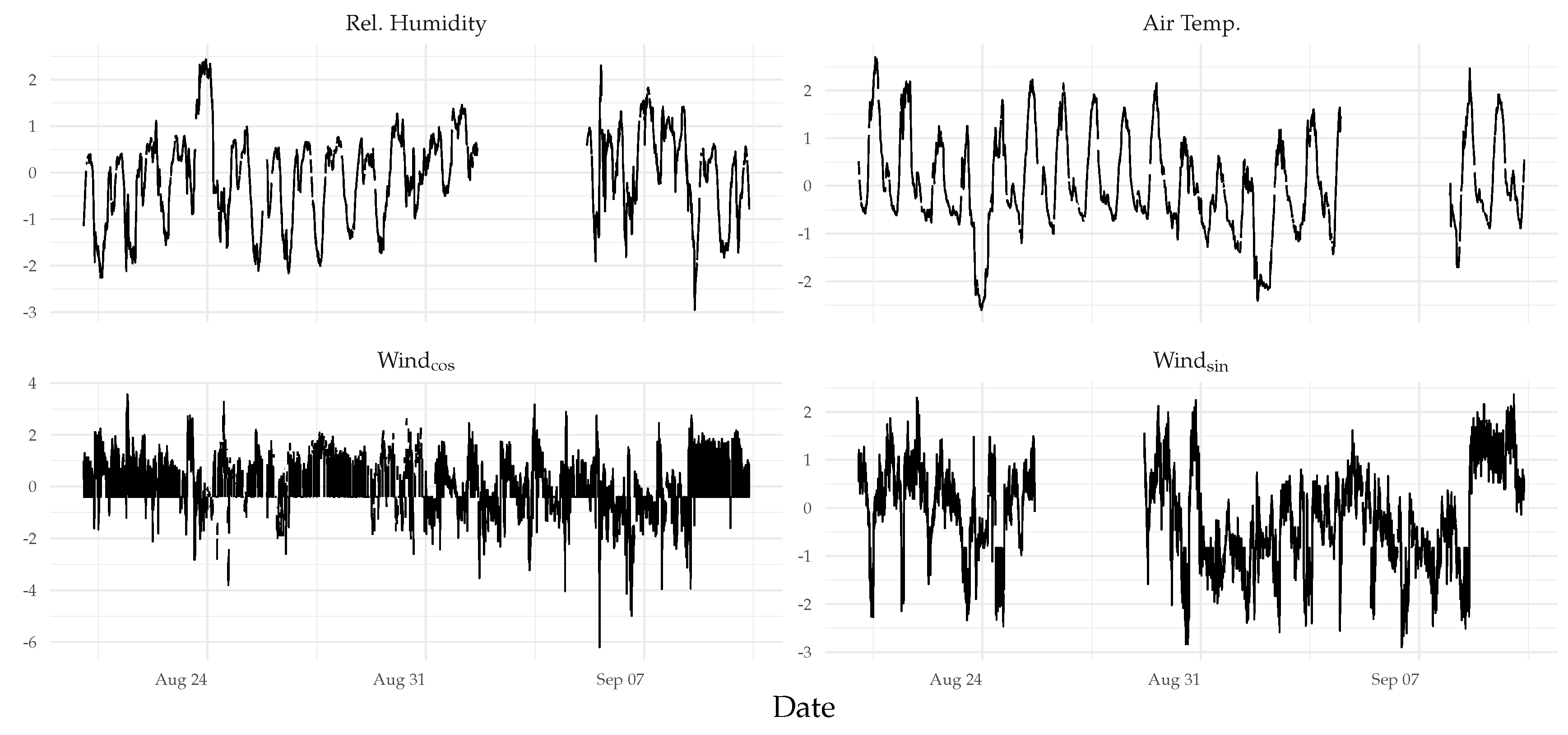
Table 8.
Characterization of the artificial missingness scenario at each station, after resampling both records to a common 15-min grid. Columns 3–6 report the number of masked cells per target variable; the two UCC variables without a contiguous block are marked with an asterisk. For humidity and at UCC, this count is the 672-sample block plus a reduced scattered contribution (24 and 14 cells, not the full /41 cells), because about a third of the independently drawn scattered positions fall inside the block window itself and add no new masked cell (see text).
Table 8.
Characterization of the artificial missingness scenario at each station, after resampling both records to a common 15-min grid. Columns 3–6 report the number of masked cells per target variable; the two UCC variables without a contiguous block are marked with an asterisk. For humidity and at UCC, this count is the 672-sample block plus a reduced scattered contribution (24 and 14 cells, not the full /41 cells), because about a third of the independently drawn scattered positions fall inside the block window itself and add no new masked cell (see text).
| Station | Records | Air Temp. | Rel. Humidity | Total masked | Block length | Variables with a block | ||
|---|---|---|---|---|---|---|---|---|
| UCC | 2049 | 31* | 696 | 686 | 41* | 1454 (17.7%) | 672 samples (7 d) | Humidity, only |
| CUC | 6251 | 786 | 777 | 769 | 796 | 3128 (12.5%) | 672 samples (7 d) | All four variables |
3.2. Imputation Accuracy
Table 9 summarizes the five decision criteria by model family, and Figure 9 details the error per target variable. Neural networks were the most accurate family on average: their median MAE (0.63 in the station-averaged matrix) was 25% lower than that of the naïve methods (0.84) and 22% lower than that of TRMF (0.81), although the family also contains the single worst alternative of the study (CSDI, discussed below). The best individual, single-station models were TKAN at UCC (MAE 0.462, RMSE 0.609) and Informer at CUC (MAE 0.491, RMSE 0.700), which reduced the MAE of the Mean imputer (0.837 at UCC and 0.815 at CUC) by 45% and 40%, and its RMSE (1.008 and 0.974) by 40% and 28%, respectively. 42 of the 46 models at UCC and 37 at CUC obtained a lower MAE than the Mean imputer. These two values are single-station results and are not directly comparable to the neural-network MAE range of Table 9 (0.48–3.83), which is computed on the station-averaged matrix (the mean of each model’s UCC and CUC MAE): TKAN’s own station-averaged MAE is 0.498 and Informer’s is 0.485, both inside that range, as is the range’s minimum (US-GAN, 0.484 station-averaged).
Because the UCC missingness scenario is asymmetric across variables, the per-variable errors are not directly comparable between temperature/ (short, scattered gaps) and humidity/ (7-day block) at that station. At UCC, the best per-variable MAE was 0.038 for air temperature and 0.434 for (both linear interpolation, reflecting the ease of bridging one- or two-sample gaps), against 0.367 for humidity (TKAN) and 0.535 for (TimeMixer) under the 7-day block. At CUC, where all four variables share the same 7-day-block scenario, the best per-variable MAE ranged from 0.261–0.312 (temperature and humidity, both BRITS) to 0.559–0.664 ( and , US-GAN and TKAN), indicating that, under a comparable gap regime, the wind components remain harder to reconstruct than the thermodynamic variables, consistently with the discussion of Section 4.3.
The diffusion-based CSDI was the clear outlier of the study: MAE 6.659 (RMSE 12.219) at UCC and 1.006 (RMSE 1.934) at CUC, both the worst results at their respective stations by a wide margin, under the common 50-epoch training budget. Naïve methods behaved unevenly depending on the gap regime: linear interpolation obtained an MAE of 1.294 for air temperature at CUC (7-day block), clearly worse than the Mean imputer (0.802) at that station, because it bridges seven days using only the two boundary values, whereas the same method obtained an MAE of only 0.038 for the same variable at UCC, where the gaps are isolated. LOCF/NOCB followed the opposite pattern (MAE 0.742 at CUC versus 1.161 at UCC), because it is best suited to short gaps and, at UCC, is dragged down by the long humidity and blocks that it can only carry forward from a single boundary value.
3.3. Edge Resource Consumption
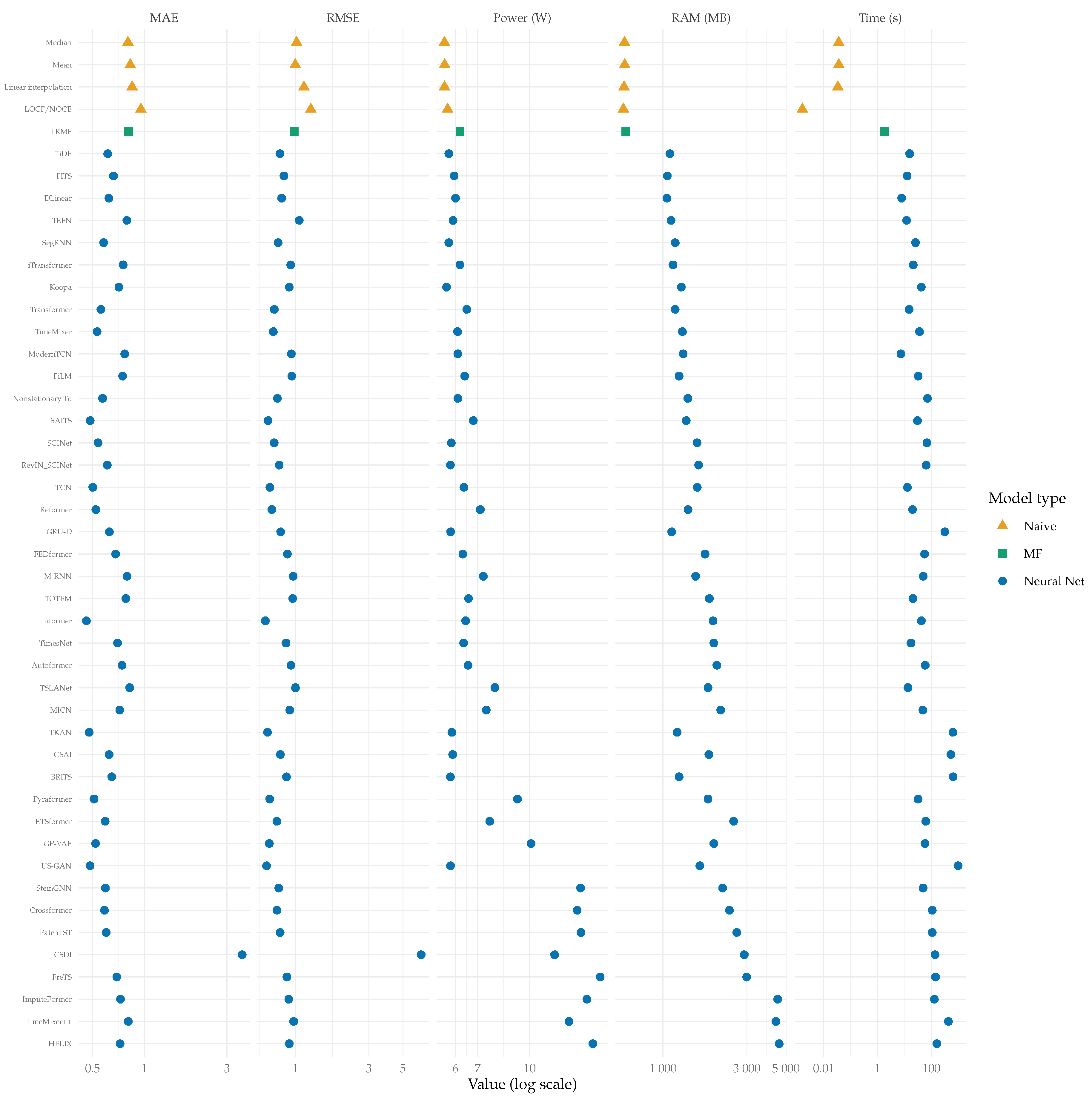
Resource usage varied by several orders of magnitude (Table 9 and Figure A1). The naïve methods and TRMF were essentially free: about 0.6 GB of RAM (593–617 MB, essentially the footprint of the Python process itself), an average power of 5.5–5.8 W (the idle baseline of the board is 5.08 W) and total times between 1.2 ms (LOCF/NOCB) and 1.0 s (TRMF). The median neural network required 1.5 GB of RAM, 6.35 W and 34.5 s (station-averaged values, Table 9). The heaviest models were also the most extreme in power: ten models exceeded 10 W in at least one station (CSDI, Crossformer, FreTS, GP-VAE, HELIX, ImputeFormer, PatchTST, StemGNN, TimeMixer++ and TimesNet), with a maximum average power of 15.8 W for FreTS at CUC. Three models exceeded 4 GB of RAM (FreTS, HELIX and TimeMixer++), and TimeMixer++ reached 5.97 GB at UCC, 78% of the 7.6 GB available on the board, with a net energy of up to 8.1 kJ per run (at CUC). Five models needed more than 300 s (BRITS, CSAI, TKAN, TimeMixer++ and US-GAN), up to 1537 s for US-GAN at CUC. The number of parameters ranged from 808 (FITS) to 6.19 million (StemGNN), with a median of 73,746 among the neural models.
Time was dominated by training. The median share of the inference call in the total time was 0.17%; the median neural network needed only 0.05 s to impute an entire series, and the slowest inference was 6.3 s (CSDI) (Figure 12). The criteria were only weakly related to each other across models (Spearman correlation over the 46 alternatives, station-averaged matrix): MAE and RMSE were almost perfectly correlated (), Power and RAM were strongly correlated (), and RAM and Time moderately (), whereas accuracy was practically unrelated to power and memory () and only weakly related to time ( to ). In other words, spending more energy or memory did not buy a better imputation in this experiment.
The Pareto fronts in Figure 10 and Figure 11 show the resulting trade-off between accuracy (RMSE) and cost (time or power), computed separately for each station. Across the six accuracy-cost fronts examined (time, power and RAM at each station), the Mean imputer was Pareto-efficient in five of six, and LOCF/NOCB, Median, DLinear and TKAN were each efficient in four of six; TCN and US-GAN were efficient in three, and TiDE, informative at the multi-criteria ranking stage, appeared in only two of the six fronts (the CUC power and RAM fronts), since it is dominated on accuracy alone at UCC by cheaper alternatives such as DLinear. Among the models that exceed 10 W or 4 GB, only GP-VAE (10.57 W at CUC) appeared in a front (accuracy versus time at CUC); none of the remaining nine heavy models (Crossformer, CSDI, FreTS, HELIX, ImputeFormer, PatchTST, StemGNN, TimeMixer++, TimesNet) was ever Pareto-efficient with respect to RMSE.
3.4. Criteria Weights
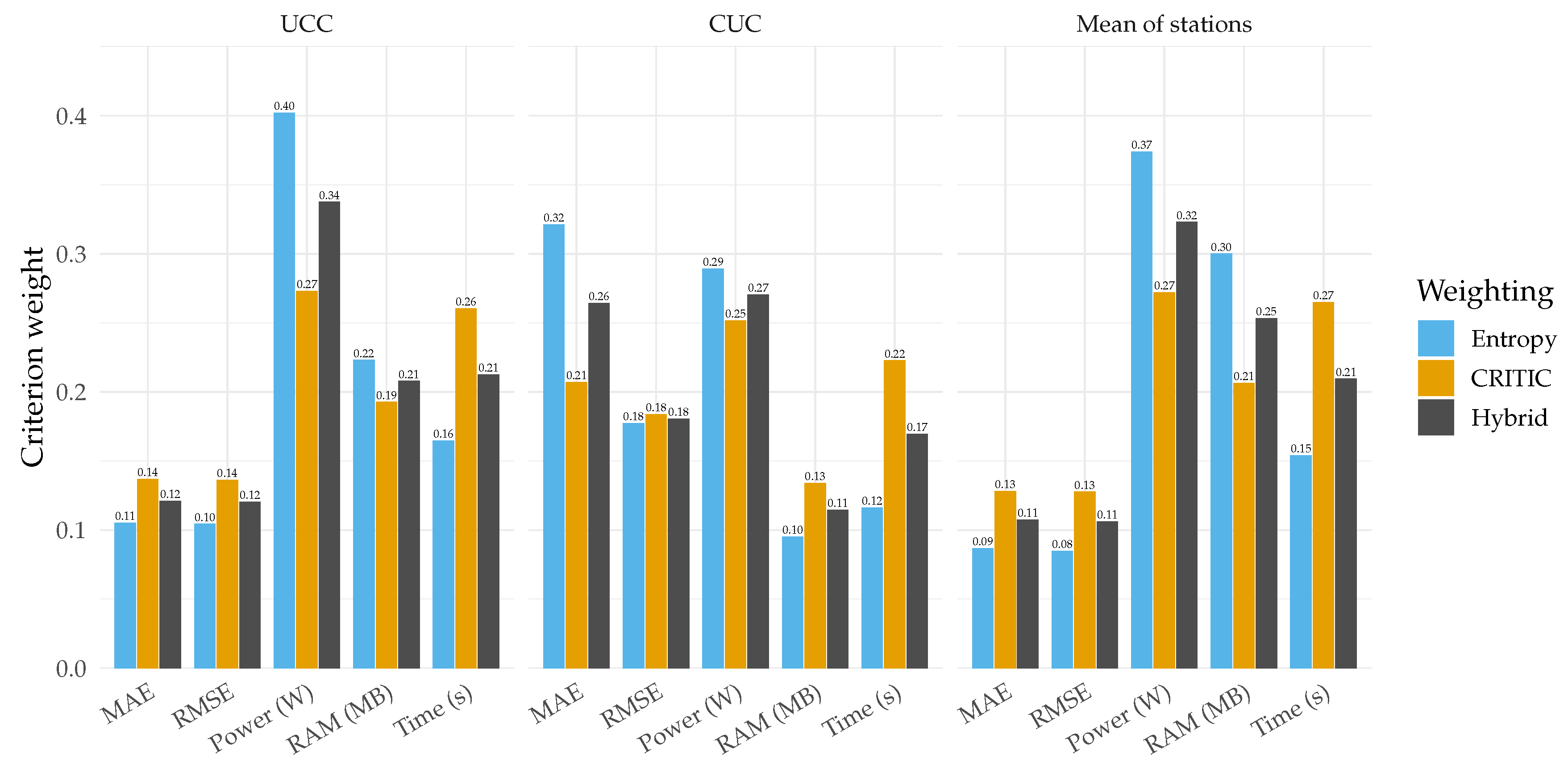
Entropy and CRITIC agree that Power and Time carry the most discriminating information among the 46 alternatives, but they disagree sharply on how much more: in the station-averaged matrix, Entropy assigned 43.9% of the total weight to Power alone (Table 10, Figure 13), against 28.0% for CRITIC, because the relative dispersion of Power once expressed as a probability distribution over the 46 alternatives is more uneven than its coefficient of variation alone suggests; RAM and Time received comparable but smaller shares from both methods (16.8–27.2%), and MAE and RMSE received the smallest Entropy weights (9.9–10.1%), lower even than the corresponding CRITIC weights (13.6% each), because they are almost perfectly redundant with each other and their normalized values are more concentrated across the 46 alternatives than those of the resource criteria, even though every criterion spans the same [0, 1] interval once min–max normalized. The hybrid weights () therefore placed 76.3% of the total weight on the three edge criteria in the station-averaged matrix and only 23.7% on accuracy, because neither Entropy nor CRITIC has any built-in preference for accuracy over resource cost: both weight a criterion solely by how much its observed values vary across the 46 alternatives. The weights at UCC were nearly identical to those of the station-averaged matrix (76.1% resources), whereas at CUC the split was less extreme (64.0% resources, 36.0% accuracy) because the accuracy differences among alternatives were more dispersed at that station, raising both the Entropy and the CRITIC weight of MAE (27.5% and 21.1%, respectively, versus 10.1% and 13.8% at UCC). Because both methods normalize the five weights of a station to sum to one (Equations (11) and (14)), this rise in the accuracy share at CUC is mirrored by a fall elsewhere, mainly in Power: its Entropy weight drops from 44.0% at UCC to 34.3% at CUC (Table 10), the complementary side of the same station-dependent redistribution rather than an independent effect.
Figure 12.
Training time versus inference time of one full-series imputation call (logarithmic axes).
Figure 12.
Training time versus inference time of one full-series imputation call (logarithmic axes).
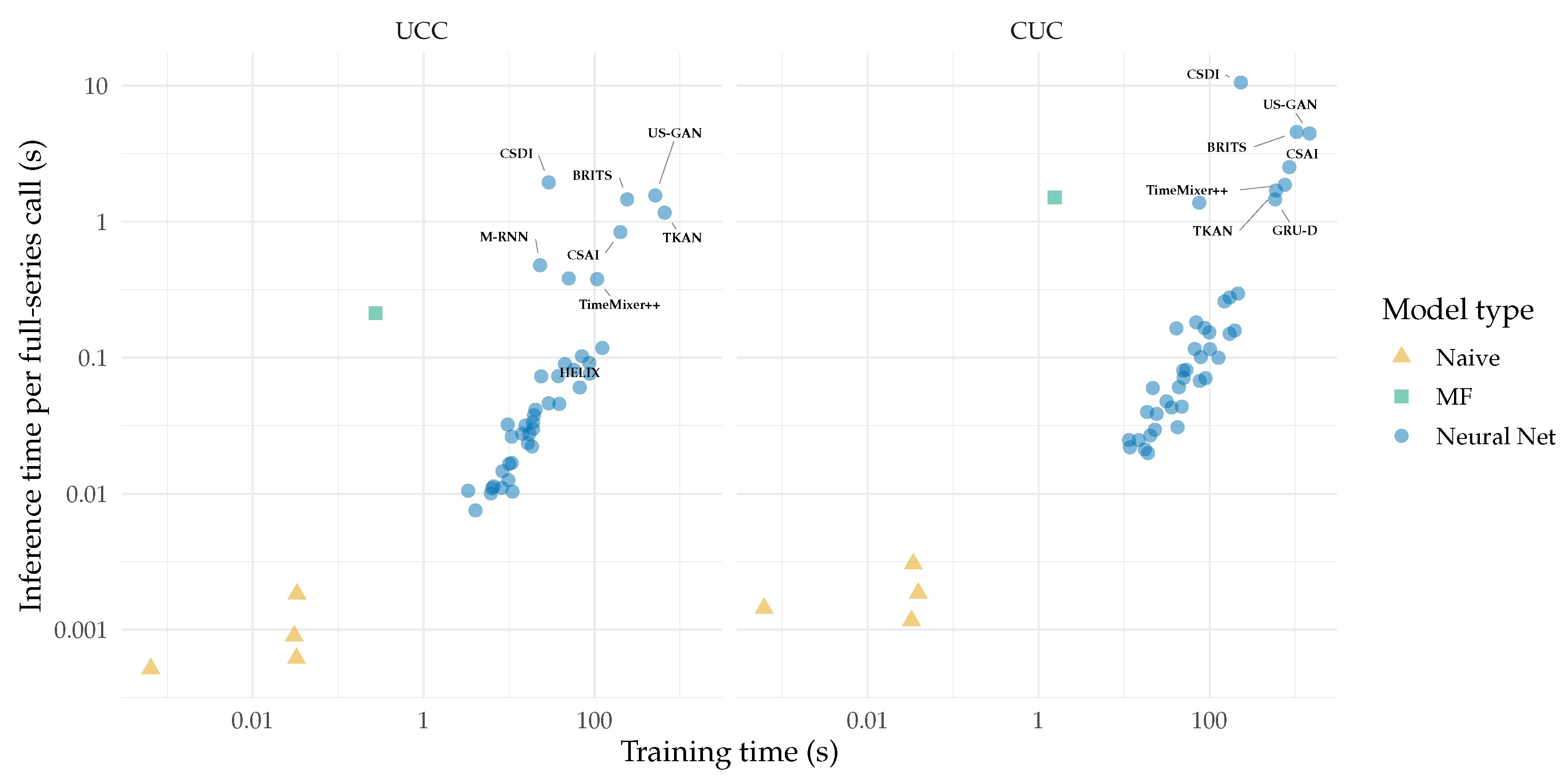
Figure 13.
Criteria weights obtained with Entropy, CRITIC and the hybrid scheme () for each station and for the station-averaged decision matrix.
Figure 13.
Criteria weights obtained with Entropy, CRITIC and the hybrid scheme () for each station and for the station-averaged decision matrix.
3.5. Multi-Criteria Ranking
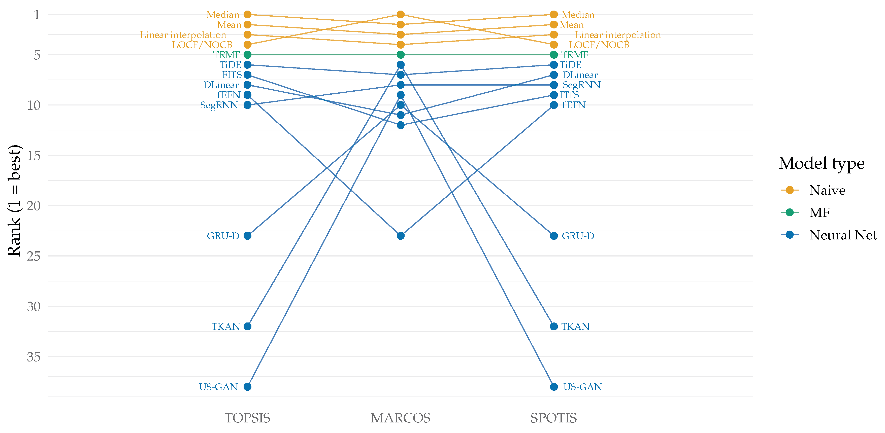
Table 11 and Figure 14 present the ranking for the station-averaged matrix. TOPSIS ranked Median first (closeness 0.974), followed by Mean (0.973), TRMF (0.969), linear interpolation (0.969) and LOCF/NOCB (0.959); TiDE was the highest-ranked neural network, in sixth place (0.957). MARCOS ranked LOCF/NOCB first (0.855), well ahead of Mean and Median (0.678 each); and SPOTIS ranked Median first (0.019), followed closely by Mean (0.019) and TRMF (0.027). The four naïve baselines and TRMF thus occupy the top five positions of both TOPSIS and SPOTIS in the station-averaged matrix, a direct consequence of the heavily resource-weighted hybrid scheme (76.3% of the weight on Power, RAM and Time; Section 3.4), for which these five alternatives are the cheapest by construction. TiDE was the highest-ranked neural network in all three methods simultaneously (ranks 6, 8 and 6 in TOPSIS, MARCOS and SPOTIS respectively), combining an MAE of 0.612 and an RMSE of 0.788 with 5.8 W, 1.1 GB of RAM and 14.4 s of training. The score differences at the top of TOPSIS were very small: the first ten closeness coefficients lie between 0.951 and 0.974. The ranking tail was fully consistent across methods and across the three decision matrices (station-averaged, UCC and CUC): HELIX, FreTS, TimeMixer++ and CSDI occupied the last four positions in every case, with TimeMixer++ last in the station-averaged and UCC matrices and CSDI last at CUC. This station-averaged picture, however, blends two markedly different regimes: as detailed next, the individual UCC and CUC rankings reorder substantially relative to each other and relative to the average, a direct consequence of the station-dependent gap structure described in Section 3.1 and quantified further in Section 3.7.
The station-specific rankings again placed the naïve methods and TRMF at the top, but with a different internal order (Table 12). At UCC, linear interpolation, Median, Mean, TRMF and LOCF/NOCB occupied the first five positions of TOPSIS, and iTransformer was the first neural network, in sixth place; this is consistent with the fact that, at that station, two of the four target variables (temperature, ) carry only short, easily interpolated gaps. At CUC, in contrast, all ten best alternatives were neural networks, led by SCINet (TOPSIS 0.929), which was also first in SPOTIS and second in MARCOS; TimeMixer, TiDE, SegRNN and TCN completed the TOPSIS top five. In MARCOS, LOCF/NOCB was first at both stations (0.836 at UCC and 0.818 at CUC), reflecting its negligible power, memory and time cost rather than its accuracy.
Figure 15.
Rank of the models that reach the top ten in at least one method (station-averaged matrix).
Figure 15.
Rank of the models that reach the top ten in at least one method (station-averaged matrix).
3.6. Agreement Between Ranking Methods and Sensitivity to the Weighting Coefficient
The rankings of TOPSIS and SPOTIS were almost identical (Spearman for the station-averaged matrix, 0.992 at UCC and 0.981 at CUC), and MARCOS now agreed moderately to closely with both (Figure 16): with TOPSIS and 0.819 with SPOTIS in the station-averaged matrix, 0.728 and 0.765 at UCC, and 0.678 and 0.752 at CUC. This close agreement arises because Entropy and CRITIC place a similarly large share of the total weight on the resource criteria, whereas MARCOS’s ratio-based normalization is itself dominated by the same criteria; the three methods therefore converge closely on the same cost-driven ordering.
The sensitivity to is shown in Figure 17 and Figure 18. The ranking was highly stable: for , the Spearman correlation with the baseline ranking () was never below 0.97 in any matrix or method (minimum 0.970 for TOPSIS at CUC; all other minima above 0.98)—an expected consequence of blending two objective methods that already agree on which criteria matter most. The identity of the best model was correspondingly almost invariant to . In the station-averaged matrix, TOPSIS selected Median for every value of tested, and SPOTIS selected Median for and Mean (with an almost identical SPOTIS score to Median) for ; MARCOS selected LOCF/NOCB throughout. At UCC, TOPSIS selected linear interpolation and MARCOS selected LOCF/NOCB for every value of , while SPOTIS selected linear interpolation for and Mean thereafter. At CUC, all three methods were completely insensitive to : TOPSIS and SPOTIS selected SCINet and MARCOS selected LOCF/NOCB at every point of the grid. The only movement observed anywhere in the sensitivity analysis was thus a tie-break between three near-identical naïve alternatives (Median, Mean and linear interpolation), never a change between a naïve method, TRMF and a neural network.
3.7. Consistency Across Stations
The agreement between the rankings of the two stations was limited for the accuracy-driven methods (Figure 19). The Spearman correlation between the UCC and CUC rankings was 0.52 for TOPSIS, 0.63 for SPOTIS and 0.93 for MARCOS. The differences concentrated on the models most affected by the asymmetric UCC missingness scenario: the naïve methods and TRMF, favoured at UCC by the short gaps in two of its four variables, ranked in the top four of TOPSIS at UCC but 26th–38th at CUC (Median: 2nd at UCC, 26th at CUC; TRMF: 4th and 30th; Mean: 3rd and 29th; linear interpolation: 1st at UCC but last but one, 38th, at CUC); conversely, SCINet, which is well suited to the uniform 7-day-block regime, ranked 17th at UCC but first at CUC. Among neural networks not directly favoured by either regime, TiDE was the most rank-stable alternative overall: across the nine rankings (three methods × three decision matrices), its rank never exceeded 12 (mean matrix: 6th/8th/6th; UCC: 9th/12th/9th; CUC: 3rd/5th/2nd), consistently placing it inside or just outside the top ten regardless of station or method; TimeMixer was a close second, never below 14th (mean matrix: 13th/10th/12th; UCC: 14th/9th/12th; CUC: 2nd/9th/4th). This benchmark used a single common configuration for every neural network; Appendix C repeats the station rankings after per-model hyperparameter tuning and finds that TiDE’s rank stability is preserved, but that tuning reorders which specific neural networks lead at CUC and makes the two stations’ rankings somewhat less, not more, mutually consistent.
4. Discussion
4.1. Main Findings
The results confirm that no single imputation model dominates when statistical accuracy and edge constraints are considered together, in line with previous benchmarks reporting that the best method depends on the missingness pattern and the deployment environment [27,28]. On the accuracy side, the benefit of learning-based imputation is clear: the best neural models reduced the MAE of the Mean imputer by 40–45% and its RMSE by 28–40% at each station, and, at CUC, all ten most accurate models were neural networks. On the resource side, however, the cost of that benefit is far from uniform. The median neural network required roughly 2.5 times the RAM, about 1.15 times the power (relative to 5.5 W for the naïve methods) and roughly a thousand times the time of the naïve methods, and the correlation between resource usage and error across the 46 alternatives was close to zero for power and memory (). Heavier models were thus not systematically better: TimeMixer++, FreTS and HELIX exceeded 4 GB of RAM and 14 W (station-averaged values) yet reached MAE values of 0.65–0.83, clearly worse than Informer (0.485, 2.1 GB, 6.4 W) or TKAN (0.498, 1.2 GB, 5.8 W). Lightweight architectures such as FITS, designed to work with very few parameters [40] (808 parameters in our configuration), DLinear [41] and the MLP-based TiDE [42] obtained MAE between 0.61 and 0.74 with roughly 1.06–1.09 GB of RAM and 8–14 s of training.
4.2. Why Simple Baselines Dominate the Multi-Criteria Ranking
Entropy and CRITIC quantify statistical dispersion and redundancy in the observed decision matrix, not practical importance assigned by a decision maker; the naïve methods and TRMF are therefore better described as the highest-ranked alternatives under this data-derived objective weighting scheme than as the “optimal” models in any absolute sense. Framed this way, the central finding of this section is that, when criterion importance is inferred exclusively from the dispersion and redundancy of the measured decision matrix, hardware-resource variability dominates the multi-criteria ranking despite the substantially better accuracy of several neural models. A notable result is that Median, Mean, TRMF and linear interpolation occupy the top four positions of TOPSIS in both the station-averaged matrix and at UCC, and that LOCF/NOCB is first in MARCOS at every matrix, although their MAE (0.80–0.95, station-averaged) is far higher than that of the most accurate alternative overall, US-GAN (MAE 0.484). This follows directly from the objective weighting scheme adopted in Section 2.6.1: with neither Entropy nor CRITIC assigning any deliberate preference to accuracy, the hybrid weights place 76.3% of the importance on the three edge criteria in the station-averaged matrix, for which the naïve methods and TRMF are the best or near-best alternatives by construction. A second, compounding factor is that the min–max normalization of Equation (12) is sensitive to extreme values: the poor result of CSDI (station-averaged MAE 3.83 and RMSE 7.08) stretches the range of both accuracy criteria so that 87% of the models obtain a normalized MAE above 0.9. The accuracy differences that matter in practice (MAE 0.48 to 0.95 outside CSDI) are thus compressed into a narrow band of the normalized scale and contribute little to the closeness coefficient even before the resource-heavy weights are applied, which explains why the ten best TOPSIS scores differ by less than 0.023 (0.951–0.974). This compression also explains why US-GAN, despite its top accuracy, does not appear in the mean-matrix top ten: at 1014.7 s it is also the second-slowest model overall, so its advantage on MAE and RMSE is outweighed once all five criteria are combined. The ranking positions within this closely spaced group should therefore be interpreted as ties rather than as strict preferences, and the shortlist—rather than a single top model, and certainly not the identity of whichever naïve method happens to edge out the others by a few thousandths of a TOPSIS point—is the robust outcome of the analysis; a decision maker who instead wants the ranking to foreground accuracy differences of this kind should either lower the resource weights manually or consult the accuracy-only comparison of Section 3.2 directly.
4.3. Effect of the Gap Structure and of the Station
The asymmetric UCC missingness scenario was not a planned experimental factor but the byproduct of applying the identical PyGrinder configuration to a series that was both shorter and already partially incomplete before masking; rather than an anomaly to discard, it provides a direct, within-station illustration of how gap length shapes imputation difficulty. At UCC, air temperature and carry only isolated one- or two-sample gaps, and simple linear interpolation is nearly exact for temperature (MAE 0.038) and competitive for (MAE 0.434); LOCF/NOCB performs almost as well (MAE 0.101 and 0.490). For the same station’s humidity and , which instead carry the 7-day block, the same naïve methods degrade sharply (linear interpolation: MAE 1.014 and 0.632; LOCF/NOCB: 1.644 and 0.758), because bridging a week-long gap from a single boundary value or a straight line is a poor approximation of the diurnal and synoptic variability of the signal. The comparison across stations reinforces this: air temperature under the 7-day block at CUC has a linear-interpolation MAE of 1.294 (versus 0.038 at UCC under short gaps), and even the best neural network for that variable and gap regime (BRITS, MAE 0.261 at CUC) remains roughly seven times worse than simple interpolation of the short UCC gaps. In the long-gap regime, no observed value of the target variable is available inside most 96-sample input windows, so the models can essentially exploit only the calendar features (hour and day of year) and the three other channels; this is consistent with the neural models achieving their best long-gap results in the thermodynamic variables, which follow a strong diurnal cycle (temperature and humidity MAE 0.26–0.37 at both stations’ long-gap variables), and comparatively worse results in the wind components ( and MAE 0.52–0.66), which are less predictable from the time of day alone.
The station effect on the multi-criteria ranking (Figure 19) is therefore confounded with this scenario difference: it cannot be attributed solely to the sampling design (both stations now share a common 15-min grid and window length, Section 2.5) or to record length (65 days at CUC versus 21 days at UCC) without also accounting for the fact that half of the UCC target variables face a much easier imputation task than any CUC variable. This may explain why SCINet, which models multi-resolution temporal structure [43] and is well suited to the uniform long-gap regime, ranked first at CUC (where all four variables share that regime) but only 16th at UCC (where it must also compete with trivially accurate short-gap interpolation). The MARCOS ranking, which is dominated by resource costs that are almost identical at both stations regardless of the missingness scenario, was the most stable across stations (), whereas the accuracy-sensitive TOPSIS ranking was the least stable (), consistent with accuracy—not resource cost—being the criterion driven by the scenario asymmetry.
4.4. Disagreement Between MARCOS and TOPSIS/SPOTIS
The moderate-to-close agreement of MARCOS with the other two methods (–0.82 depending on the matrix) is a consequence of how each method normalizes criteria that span several orders of magnitude, not of an error in the computation; it arises precisely because the resource-heavy Entropy/CRITIC weights push TOPSIS and SPOTIS towards the same cost-dominated alternatives that MARCOS already favours. The time criterion ranged from 1.7 ms to 1014.7 s in the station-averaged matrix (up to 1537 s at CUC alone). MARCOS normalizes cost criteria by the ratio between the best value and the alternative’s value, so 91% of the alternatives obtained a normalized time below 0.01 and only the four naïve methods retained a meaningful score on this criterion; LOCF/NOCB, the best or near-best alternative in Power, RAM and Time simultaneously, therefore approached the ideal solution and ranked first (0.855 versus 0.678 for the joint second-placed Mean and Median) even though its MAE (0.951) is 96% higher than that of the single most accurate model, US-GAN (0.484), and 15% higher than the Mean imputer’s own MAE (0.826). TOPSIS and SPOTIS use range-based distances that compress the same criterion in the opposite direction: 85% of the alternatives obtained a normalized time above 0.9. The two families of methods thus encode different attitudes towards large relative differences among cheap alternatives, and the choice between them should be made explicitly by the decision maker. Regarding SPOTIS, its invariance to rank reversal [39] depends on defining the bounds of each criterion independently of the alternatives; in this study, the bounds were the observed minima and maxima, so this property was not fully exploited and the SPOTIS ranking should be considered a robustness check of the TOPSIS ranking (with which it agrees closely, in every matrix) rather than an independent confirmation.
4.5. Practical Guidance for Edge Deployment
Within the scope of this dataset and configuration, the results suggest the following options. (i) If the memory, energy or latency budget is very restrictive, or training on the device is not possible, the naïve methods and TRMF are not just viable but are, under the objective weighting scheme adopted here, also the top-ranked alternatives overall (about 0.6 GB, 5.5–5.8 W, 1.7 ms to 1.0 s), accepting an MAE of 0.80–0.95 in z-score units, with the caveat that their accuracy depends strongly on the gap length actually encountered and that a decision maker who values accuracy more than the resource criteria weight it here should consult Section 3.2 directly rather than the multi-criteria ranking alone. (ii) As the best-performing neural network under both accuracy and stability, TiDE offers a 26% lower MAE than the Mean imputer (0.612 versus 0.826, station-averaged) with about 1.1 GB of RAM, 5.8 W and 14 s of training, was the highest-ranked neural network in all three multi-criteria methods and was the most rank-stable alternative overall across stations and methods; TimeMixer is a close second on stability and offers the lowest MAE among the lightweight neural networks (0.531, a 36% reduction versus the Mean imputer) with about 1.3 GB of RAM, 6.1 W and 36 s of training; FITS and DLinear are lighter still (8.0 s of training, about 1.06 GB) at the cost of a somewhat higher error (MAE 0.62–0.74). (iii) If accuracy is the priority, TKAN was the most accurate model at UCC (MAE 0.462, 1.2 GB, about 3.5 min of training), and Informer (MAE 0.491, 2.1 GB, 37 s) and SCINet (MAE 0.494, 1.6 GB, 90 s) were the best choices at CUC; US-GAN obtained the single best station-averaged MAE (0.484) but required 1015 s of training on average (up to 1537 s at CUC), which may be prohibitive if the model must be retrained on the device. (iv) CSDI, FreTS, HELIX and TimeMixer++ should be avoided under the configuration evaluated here, because they combine large memory (4.2–5.8 GB) or power (14.7–15.6 W) with no accuracy advantage over much cheaper alternatives, or, in the case of CSDI, markedly unstable results (MAE 6.66 at UCC versus 1.01 at CUC). (v) All of the above used the common compact configuration of Section 2.5; a practitioner willing to run the per-model search of Appendix C on their own device before committing to a model should expect UCC’s recommendation to be essentially unaffected, but CUC’s to shift towards a different subset of neural networks (SAITS, Informer, TCN, Reformer and SegRNN) and away from the naïve methods and TRMF even more strongly than already observed here.
4.6. Limitations and Future Work
This study has limitations that constrain the generality of the conclusions. The two most consequential are listed first.
- 1.
- Asymmetric UCC missingness scenario. Only relative humidity and received the intended 7-day contiguous block at UCC; air temperature and received only scattered short gaps, because the CUC PyGrinder configuration was applied to a UCC record that was both shorter (2049 versus 6251 samples) and already partially incomplete before masking. This confounds the station comparison of Section 4.3 with a scenario-difficulty difference and should be resolved—by regenerating a symmetric UCC scenario, or by explicitly reframing the mixed short/long-gap design as intentional—before the station-level conclusions are finalized.
- 2.
- No individual hyperparameter tuning in the main benchmark. All 46 models were evaluated with a common compact configuration and a fixed 50-epoch budget, which may penalize models that need longer training (CSDI in particular, also the least stable model across stations). Appendix C repeats the ranking after per-model tuning and reports where the conclusions do, and do not, change.
- 3.
- Limited statistical power. Only two stations and short records (21.3 and 65.1 days) were used, with a single missingness realization and a single training seed, so no confidence intervals could be estimated and small differences among neighbouring models are not statistically established.
- 4.
- Training-dominated time criterion. Training time accounted for a median of 99.83% of the measured time budget. This is a defensible choice for the comparison performed here, since it is the cost actually incurred when a model must be fitted and used directly on the device without a separate training platform, but it does not represent the most common edge-deployment pattern, in which training happens offline and only inference latency and energy matter at the edge; under that pattern, which this study does not evaluate, the time ranking—and hence the multi-criteria ranking for cost-sensitive alternatives—would change substantially, since inference alone accounted for a median of only 0.17% of the measured time (Section 3.3).
- 5.
- Transductive protocol. Imputation accuracy was evaluated within the training record, not as generalization to future, unseen data.
- 6.
- Hardware measurement caveats. Power was measured at the board input (INA3221 monitor, including carrier-board overheads) and RAM combines process and reserved GPU memory; the measurement window was adaptively extended to at least 3 s per phase, but single-run measurements remain subject to the thermal and scheduling variability of the shared board.
- 7.
- Normalization choice in the MCDM stage. The objectively derived weights still depend on the min–max normalization of Equation (12), which compresses the accuracy criteria relative to the resource criteria and drives the naïve methods and TRMF to the top of the ranking; a decision maker who wants accuracy to dominate should reweight the criteria manually or apply an outlier-robust normalization, neither of which was evaluated here.
- 8.
- Hyperparameter-search coverage and variance. The random-search protocol of Appendix C (8 trials per model and station) produced a valid tuned configuration for 94% of the tunable combinations and occasionally selected a configuration that generalized worse than the common one; a larger budget or a more sample-efficient search (e.g., Bayesian optimization) could close the remaining gap and reduce this variance.
Future work should regenerate a symmetric missingness scenario at both stations, include more stations and gap lengths, repeated runs with several seeds, a larger-budget or Bayesian variant of the hyperparameter search of Appendix C, inference-only measurements of pre-trained models, and the evaluation of outlier-robust normalization schemes for the MCDM stage.
5. Conclusions
This study evaluated 46 time-series imputation models from the PyPOTS ecosystem on two meteorological stations of the Colombian Caribbean coast, running on an NVIDIA Jetson Orin Nano (25 W mode), and ranked them with a hybrid Entropy–CRITIC weighting—both methods fully objective and derived directly from the measured decision matrix—followed by TOPSIS and MARCOS, with SPOTIS used as an additional ranking-consistency check. Neural networks reduced the imputation error of the Mean imputer by 40–45% (MAE) and 28–40% (RMSE), but the resource cost varied by orders of magnitude and did not correlate with accuracy: several of the most demanding models (up to 5.97 GB of RAM and 15.8 W) were among the least accurate. Because Entropy and CRITIC placed 64–76% of the total weight on the three edge-resource criteria depending on the matrix, the naïve baselines and TRMF—the cheapest alternatives by construction—topped the TOPSIS, SPOTIS and MARCOS rankings in the station-averaged matrix and at UCC; among neural networks, TiDE was the most rank-stable alternative overall, never ranking below 12th across the three ranking methods and the three decision matrices (station-averaged, UCC, CUC), with a favourable balance of accuracy (MAE 0.61), memory (1.1 GB), power (5.8 W) and training time (14 s), and TimeMixer was a close second in stability with the lowest MAE (0.53) among the lightweight neural networks. The best model at each station according to TOPSIS differed markedly (Median-family naïve methods at UCC and SCINet at CUC under the common, untuned configuration—Appendix C shows tuning reorders the CUC top), but the top-ranked model was almost completely insensitive to the Entropy/CRITIC weighting coefficient (Spearman correlation with the baseline never below 0.97), so the shortlist obtained from the analysis is a stable, not merely a robust, outcome. TOPSIS and SPOTIS agreed almost perfectly (), and MARCOS agreed moderately to closely with both (–0.82), a close three-way agreement because all three methods are driven by the same objectively resource-heavy criteria structure. Station-to-station agreement was low for the accuracy-driven rankings ( for TOPSIS); this low value is not interpretable as a genuine station effect, since the artificial missingness scenario realized at UCC was asymmetric across variables—a 7-day gap in two of the four targets and only short, scattered gaps in the other two—rather than uniform as at CUC, confounding the station comparison, so the resulting station-level conclusions are not directly comparable. This asymmetry most plausibly arose because the identical PyGrinder configuration was applied to a UCC record that was both shorter and already partially incomplete before masking, unlike the longer and originally complete CUC record; resolving it is a prerequisite for a clean station-level comparison in any subsequent version of this work. A fully automated, per-model hyperparameter-search protocol and its scripts are provided in Appendix C and were run at full scale on the same device: tuning improved MAE by 2.8% on average across 79 of the 84 tunable model–station combinations searched successfully, left the UCC ranking practically unchanged, but reordered the top of the CUC ranking around a different set of neural networks (SAITS, Informer and TCN replacing SCINet, TimeMixer and TiDE) and pushed the naïve methods and TRMF still further down that station’s ranking, without making the two stations’ rankings any more mutually consistent. The proposed framework is nonetheless reproducible and transferable to other edge platforms and monitoring networks, and its main next steps are a symmetric re-run of the missingness scenario, repeated runs with several seeds, a larger-budget or Bayesian variant of the provided hyperparameter-search protocol to cover the remaining models and reduce outcome variance, and inference-only measurements.
Author Contributions
Conceptualization, D.R.-L., A.O.-C. and P.F.-d.-C.; methodology, D.R.-L. and M.E.I.-M.; software, D.R.-L.; validation, M.C.-R., C.R.-A. and M.E.I.-M.; formal analysis, D.R.-L. and M.C.-R.; investigation, D.R.-L., M.C.-R. and C.R.-A.; resources, A.O.-C. and P.F.-d.-C.; data curation, D.R.-L. and M.C.-R.; writing—original draft preparation, D.R.-L.; writing—review and editing, A.O.-C., C.R.-A., M.E.I.-M. and P.F.-d.-C.; visualization, D.R.-L.; supervision, A.O.-C. and P.F.-d.-C.; project administration, A.O.-C.; funding acquisition, A.O.-C. and P.F.-d.-C. All authors have read and agreed to the published version of the manuscript.
Funding
This research was funded by the Ministerio de Ciencia, Tecnología e Innovación—Fondo Francisco José de Caldas and the Agencia Nacional de Hidrocarburos (ANH), through the Contrato de Financiamiento de Recuperación Contingente No. 112721-053-2025, within the project “Herramientas tecnológicas y prototipos para caracterizar, identificar y optimizar el potencial eólico en zonas costeras de Colombia” (Project Code 111983).
Institutional Review Board Statement
Not applicable.
Informed Consent Statement
Not applicable.
Data Availability Statement
The datasets and evaluation scripts generated and analyzed during this study are publicly available on GitLab at https://gitlab.com/diegorestrepo/edge-imputation-benchmark-santamarta-barranquilla (accessed on 25 September 2026).
Acknowledgments
The authors would like to thank Universidad de la Costa, and Universidad Cooperativa de Colombia for providing access to the meteorological data. This work was supported by the Generalitat Valenciana (Spain) through PROMETEO grant CIPROM/2023/32, awarded to P.F.-d.-C.; and by the Conselleria de Educación, Cultura, Universidades y Empleo of the Generalitat Valenciana (Reference CIAPOS/2024/238, APOSTD/2025 – MODALIDAD A), co-funded by the European Social Fund Plus (FSE+) under the 2021–2027 Operational Programme of the Comunitat Valenciana, supporting M.E.I.-M.
Conflicts of Interest
The authors declare no conflicts of interest.
Abbreviations
The following abbreviations are used in this manuscript:
| AAI | Anti-Ideal Solution |
| AI | Ideal Solution |
| A.S.L. | Above Sea Level |
| BRITS | Bidirectional Recurrent Imputation for Time Series |
| CRITIC | Criteria Importance Through Intercriteria Correlation |
| CSAI | Cross-Self Attention Imputation |
| CSDI | Conditional Score-based Diffusion model for Imputation |
| CUC | Universidad de la Costa |
| CUDA | Compute Unified Device Architecture |
| DL | Deep Learning |
| DRAM | Dynamic Random-Access Memory |
| FHSS | Frequency-Hopping Spread Spectrum |
| FITS | Fast Frequency-Domain Imputation for Time Series |
| GP-VAE | Gaussian Process Variational Autoencoder |
| GRU-D | Gated Recurrent Unit with Decay |
| HPO | Hyperparameter Optimization |
| LOCF | Last Observation Carried Forward |
| LPDDR5 | Low Power Double Data Rate 5 |
| MAE | Mean Absolute Error |
| MARCOS | Measurement of Alternatives and Ranking according to Compromise Solution |
| MCDA | Multi-Criteria Decision Analysis |
| MCDM | Multi-Criteria Decision-Making |
| MDPI | Multidisciplinary Digital Publishing Institute |
| MF | Matrix Factorization |
| ML | Machine Learning |
| MLP | Multi-Layer Perceptron |
| NOCB | Next Observation Backward |
| NVIDIA | Next-Generation Visual Information Dynamics Interactive Architecture |
| PyPOTS | Python Toolkit for Machine Learning on Partially-Observed Time Series |
| RAM | Random-Access Memory |
| RMSE | Root Mean Square Error |
| SAITS | Self-Attention-based Imputation for Time Series |
| SPOTIS | Stable Preference Ordering Towards Ideal Solution |
| StemGNN | Spatial-Temporal Graph Neural Network |
| TCN | Temporal Convolutional Network |
| TDP | Thermal Design Power |
| TiDE | Time-series Dense Encoder |
| TLA | Three-Letter Acronym |
| TOPSIS | Technique for Order Preference by Similarity to Ideal Solution |
| TOPS | Trillion Operations Per Second |
| TRMF | Temporal Regularized Matrix Factorization |
| UCC | Universidad Cooperativa de Colombia |
| US-GAN | Unsupervised Sampling Generative Adversarial Network |
Appendix A
Table A1.
Statistical summary of the normalized, cleaned station dataset.
| Station | Variable | N | Valid (n) | Min | Q1 | Median | Mean | Q3 | Max | Missing (n) | Missing (%) |
|---|---|---|---|---|---|---|---|---|---|---|---|
| CUC | 6251 | 6251 | 0 | 0 | |||||||
| 6251 | 6251 | 0 | 0 | ||||||||
| 6251 | 6251 | 0 | 0 | ||||||||
| 6251 | 6251 | 0 | 0 | ||||||||
| Rel. Humidity | 6251 | 6251 | 0 | 0 | |||||||
| Air Temp. | 6251 | 6251 | 0 | 0 | |||||||
| 6251 | 6251 | 0 | 0 | ||||||||
| 6251 | 6251 | 0 | 0 | ||||||||
| UCC | 2049 | 2049 | 0 | ||||||||
| 2049 | 2049 | 0 | |||||||||
| 2049 | 2049 | 0 | |||||||||
| 2049 | 2049 | 0 | |||||||||
| Rel. Humidity | 2049 | 2030 | 19 | ||||||||
| Air Temp. | 2049 | 2037 | 12 | ||||||||
| 2049 | 2036 | 13 | |||||||||
| 2049 | 2036 | 13 |
Table A2.
Selected models supporting imputation (IMPT).
| Type | Model |
|---|---|
| Naïve | Linear interpolation |
| Naïve | LOCF/NOCB |
| Naïve | Mean |
| Naïve | Median |
| Neural Net | HELIX [44] |
| Neural Net | SegRNN [45] |
| Neural Net | TEFN [46] |
| Neural Net | TimeMixer++ [47] |
| Neural Net | TSLANet [48] |
| Neural Net | FITS [40] |
| Neural Net | TimeMixer [49] |
| Neural Net | iTransformer [50] |
| Neural Net | ModernTCN [51] |
| Neural Net | ImputeFormer [52] |
| Neural Net | TOTEM [53] |
| Neural Net | TKAN [54] |
| Neural Net | SAITS [55] |
| Neural Net | FreTS [56] |
| Neural Net | Koopa [57] |
| Neural Net | Crossformer [58] |
| Neural Net | TimesNet [59] |
| Neural Net | PatchTST [60] |
| Neural Net | ETSformer [61] |
| Neural Net | MICN [62] |
| Neural Net | DLinear [41] |
| Neural Net | TiDE [42] |
| Neural Net | CSAI [63] |
| Neural Net | SCINet [43] |
| Neural Net | Nonstationary Tr. [64] |
| Neural Net | FiLM [65] |
| Neural Net | RevIN_SCINet [66] |
| Neural Net | Pyraformer [67] |
| Neural Net | FEDformer [68] |
| Neural Net | Autoformer [69] |
| Neural Net | CSDI [70] |
| Neural Net | Informer [71] |
| Neural Net | US-GAN [72] |
| Neural Net | StemGNN [73] |
| Neural Net | Reformer [74] |
| Neural Net | GP-VAE [75] |
| Neural Net | M-RNN [76] |
| Neural Net | BRITS [77] |
| Neural Net | GRU-D [78] |
| Neural Net | TCN [79] |
| Neural Net | Transformer [80] |
| MF | TRMF [81] |
Appendix B
Figure A1.
Decision matrix for the 46 alternatives (station-averaged values, logarithmic axes). Models are sorted by TOPSIS rank, best at the top.
Figure A1.
Decision matrix for the 46 alternatives (station-averaged values, logarithmic axes). Models are sorted by TOPSIS rank, best at the top.
Appendix C
Appendix C.1. Automated Hyperparameter-Optimization Protocol
The main benchmark deliberately used a single, common compact configuration for the 41 neural networks (two layers, hidden size 64, four attention heads where applicable, 50 epochs, batch size 32), so that the resource comparison of Section 3.3 would not be confounded by unequal tuning effort across 46 heterogeneous architectures. This design choice is appropriate for a like-for-like edge-resource comparison, but it is not the configuration a practitioner would want once a specific model has been shortlisted for deployment. This appendix describes a complementary, fully automated hyperparameter-search protocol, together with the two scripts that implement it (hpo_edge.py and run_hpo_edge.sh, distributed alongside edge_impute.py), that lets any single model search for a better configuration directly on the target edge device, without requiring a machine-learning expert to hand-pick values.
Appendix C.1.1. Leak-Free Validation Split
Hyperparameter search must be scored against data that the main benchmark never uses for evaluation, otherwise the reported test accuracy of Section 3.2 would be biased. For each station, an additional validation mask is generated independently of the PyGrinder test mask , using a different pseudorandom seed (123, instead of the 42 used for ) and restricted to cells that are simultaneously (i) currently observed in the input series and (ii) not already part of :
For each of the four target variables, combines one contiguous block (384 samples, 4 days, versus the 672-sample/7-day block of the main missingness scenario) with a scattered component (3% of the remaining eligible cells), mirroring the two-part structure of the main scenario at a smaller scale so that the validation score reflects both short- and long-gap difficulty. A candidate configuration is fitted on the series with additionally hidden and scored by its MAE and RMSE on exactly those cells, whose true value is known but was hidden from the fit; itself is never touched, so the validation score cannot leak into, and is not comparable to, the test accuracy reported in Section 3.2.
Appendix C.1.2. Search Space and Algorithm
For each of the 41 neural networks and for TRMF, the search space combines (i) the numeric architecture hyperparameters already present in that model’s common-configuration dictionary that plausibly control model capacity (hidden/embedding dimensions, number of layers, number of attention heads, and, for TRMF, its rank K and iteration budget), each scaled to , and its common-configuration value, and (ii) for the neural networks, a small grid over the number of training epochs () and batch size (). This construction is generic—it reads the common-configuration dictionary of any model and infers a search space from it automatically—so it required no per-model manual tuning and covers all 42 tunable models (the four naïve baselines have no hyperparameters and are excluded). Because the resulting space ranges from a handful to several thousand combinations depending on the model (Table A3), an exhaustive grid search is not tractable within an edge-appropriate time budget; instead, a random search [82] is used, with a fixed, user-configurable budget of trials per model (8 by default), always including the common configuration itself as the first trial so that the search can never do worse than the main benchmark’s baseline. Each trial is fitted and scored independently and wrapped in exception handling, so a single failing configuration (for example, an architecturally invalid combination of heads and embedding size) is logged and skipped rather than aborting the search.
Table A3.
Size of the automatically inferred search space for a representative subset of models (see hpo_edge.py list for the full 42-model listing).
Table A3.
Size of the automatically inferred search space for a representative subset of models (see hpo_edge.py list for the full 42-model listing).
| Model | Scalable hyperparameters | Combinations | Random-search budget |
|---|---|---|---|
| TRMF | K, max_iter | 9 | 8 |
| DLinear | 36 | 8 | |
| TiDE | , , , ...(5 total) | 2916 | 8 |
| SAITS / Transformer / iTransformer | , , , , , | 8748 | 8 |
Appendix C.1.3. Scripts and Reintegration into the Main Pipeline
hpo_edge.py implements the protocol above as a self-contained command-line tool that imports edge_impute.py directly (its model registry, data loader and PyPOTS model-building routine) rather than duplicating that logic; it exposes list (prints the inferred search space per model), run –model M –station S (executes the random search for one model at one station and writes its full trial log as JSON) and aggregate (combines all per-model logs into a single hpo_trials.csv, for auditing every trial’s validation MAE/RMSE and wall-clock fit/predict time, and a best_params.json with the best configuration found per model and station). run_hpo_edge.sh orchestrates hpo_edge.py over every station and (by default) every tunable model, following the same operational safeguards already validated for run_imputation_edge.sh in the main benchmark: a preflight import check, per-model timeouts, resumability (a model/station already logged is skipped unless re-run is forced), and an explicit SMOKE=1 mode that runs a two-trial, reduced-epoch, reduced-row search over a handful of models, intended to be run first to validate the environment before committing to the full search. edge_impute.py itself was extended with an optional –hparams-file argument on its run subcommand: given a best_params.json produced by hpo_edge.py aggregate, it overrides the common-configuration hyperparameters of the named model for that one run, so that the main benchmark can be repeated with tuned, model-specific configurations (writing to a separate output directory to keep the original, common-configuration decision matrices of this article intact) and the resulting decision matrix can be re-ranked with the unmodified mcda_edge.R of Section 2.6.1.
Appendix C.1.4. Empirical Results of the Full-Scale Search
The protocol above was subsequently run at full scale on the same Jetson Orin Nano, with the default budget of 8 random trials per model and station (the common configuration always included as the first trial), producing a valid tuned configuration for 79 of the 84 tunable model–station combinations (94%; 42 tunable models × 2 stations). Five combinations completed no successful trial and therefore kept the common configuration of Section 2.5 in the tuned benchmark that follows: US-GAN at both stations, and BRITS, CSAI and TKAN at CUC only; a further twelve combinations (for example, TiDE, SAITS, DLinear and TimeMixer at UCC) completed successfully but the random search selected the common configuration itself as the best trial, so their tuned result is numerically identical to the untuned one. Across the remaining 67 combinations that were both searched successfully and produced a different configuration, MAE decreased in 42 cases and increased in 23, with a mean change of and a median of ; occasional deteriorations after tuning (worst case: SCINet at CUC, MAE) are consistent with the small per-model validation budget (8 trials, Section C.1) sometimes selecting a configuration that overfits the validation split of Equation (A1) rather than one that generalizes to the test mask , a risk inherent to random search under a tight, edge-appropriate trial budget. The largest improvement was CSDI at CUC ( MAE, RMSE), consistent with Limitation 3 that a fixed 50-epoch budget penalizes slower-converging architectures.
The effect on the multi-criteria ranking was station-dependent. At UCC, where the naïve methods and TRMF were already the top five alternatives in the untuned benchmark (Table 12), tuning left that ordering essentially unchanged (linear interpolation, Median, Mean, TRMF and LOCF/NOCB still occupy TOPSIS ranks 1–5; TiDE replaces iTransformer in sixth place). At CUC, in contrast, tuning reordered the neural networks at the top—SAITS, Informer, TCN, Reformer and SegRNN now lead TOPSIS, ahead of TimeMixer and TiDE, whereas SCINet, first in the untuned benchmark, fell to 13th after its unfavourable tuning outcome noted above—and, more strikingly, pushed the naïve methods and TRMF markedly further down the tail than they already were (Table A4): all five lost between 3 and 8 TOPSIS ranks, with linear interpolation falling from 38th to 41st of 46. MARCOS, whose score is driven mainly by resource cost rather than accuracy, kept LOCF/NOCB first at CUC both before and after tuning, since neither its own configuration nor its resource footprint changed.
Table A4.
TOPSIS and MARCOS rank of the naïve baselines and TRMF at CUC, before and after hyperparameter tuning (46 alternatives in total; lower rank is better).
Table A4.
TOPSIS and MARCOS rank of the naïve baselines and TRMF at CUC, before and after hyperparameter tuning (46 alternatives in total; lower rank is better).
| Model | TOPSIS (untuned) | TOPSIS (tuned) | MARCOS (untuned) | MARCOS (tuned) |
|---|---|---|---|---|
| LOCF/NOCB | 21 | 31 | 1 | 1 |
| Median | 26 | 32 | 4 | 12 |
| Mean | 29 | 34 | 6 | 13 |
| TRMF | 30 | 36 | 10 | 28 |
| Linear interpolation | 38 | 41 | 11 | 25 |
This CUC-specific reversal did not propagate into a more consistent cross-station ranking: the UCC–CUC Spearman correlation of the tuned TOPSIS ranking (0.32) and SPOTIS ranking (0.39) were both lower than their untuned counterparts (0.52 and 0.63, Section 3.7), because per-station tuning lets each station’s models specialize further to that station’s own missingness realization rather than converging on a common best model; MARCOS remained the most cross-station-stable method, but also declined somewhat (0.81 tuned versus 0.93 untuned). Despite this, TiDE remained the single most rank-stable alternative overall across the three methods and three decision matrices even after tuning (maximum rank 12 of 46, unchanged from the untuned benchmark, Section 3.7), reinforcing it as the recommendation of Section 3.7 that is least sensitive to whether per-model tuning is subsequently applied. Running the search itself (588 trials, 557 completed successfully) consumed approximately 8.1 hours of additional fit-plus-predict time on the Jetson beyond the main benchmark, a one-off cost incurred once per deployment decision rather than per inference.
These results should be read together with Limitation 8: the search covered 94% of the tunable model–station combinations under a modest budget (8 trials) and a single validation split, so the five uncovered combinations and the occasional unfavourable outcome (SCINet at CUC) indicate room for a larger budget or repeated validation splits in future work, rather than a definitive statement that tuning cannot help those particular models.
References
- Xavier, A.C.; Scanlon, B.R.; King, C.W.; Alves, A.I. New improved Brazilian daily weather gridded data (1961–2020). Int. J. Climatol. 2022, 42, 8390–8404. [Google Scholar] [CrossRef]
- Cedric, L.S.; Adoni, W.Y.H.; Aworka, R.; Zoueu, J.T.; Mutombo, F.K.; Krichen, M.; Kimpolo, C.L.M. Crops yield prediction based on machine learning models: Case of West African countries. Smart Agric. Technol. 2022, 2, 100049. [Google Scholar] [CrossRef]
- Jamshidi, S.; Pourhossein, K.; Asadi, M. Size estimation of wind/solar hybrid renewable energy systems without detailed wind and irradiation data: A feasibility study. Energy Convers. Manag. 2021, 234, 113905. [Google Scholar] [CrossRef]
- Liang, Y.; Wu, C.; Zhang, M.; Ji, X.; Shen, Y.; He, J.; Zhang, Z. Statistical modelling of the joint probability density function of air density and wind speed for wind resource assessment: A case study from China. Energy Convers. Manag. 2022, 268, 116054. [Google Scholar] [CrossRef]
- National Laboratory of the Rockies. System Advisor Model™ Version 2025.4.16 (SAM™ 2025.4.16). Available online: https://sam.nler.gov (accessed on 27 Aug 2026).
- Restrepo-Leal, D.; Carrillo-Reales, M. Detailed Theoretical Framework and Procedure for Wind Power Estimation and Turbine Sizing Based on Site Characterization. 2026. [Google Scholar] [CrossRef]
- Si, P.; Liao, J.; Li, Y.; Jiang, H. Quality Control and Homogeneity Analysis of Hourly Surface Air Temperature at Regional Automatic Meteorological Stations in the Tianjin Area during 2008–2023. Chin. J. Atmos. Sci. 2026, 50, 764–777. [Google Scholar] [CrossRef]
- Sládek, D.; Dohnal, F.; Paulus, F.; Neubauer, J.; Zeman, T. ML-based fire cause prediction: Integrating population mobility and meteorological data. Int. J. Disaster Risk Reduct. 2026, 143. [Google Scholar] [CrossRef]
- Coimbra, I.; Palma, J. Synoptic and mesoscale winds in the complex terrain of Perdigão. 2022, Vol. 2265. [Google Scholar] [CrossRef]
- Piasecki, A.; Jurasz, J.; Kies, A. Measurements and reanalysis data on wind speed and solar irradiation from energy generation perspectives at several locations in Poland. SN Appl. Sci. 2019, 1. [Google Scholar] [CrossRef]
- Varotsos, K.V.; Katavoutas, G.; Giannakopoulos, C. On the Use of Reanalysis Data to Reconstruct Missing Observed Daily Temperatures in Europe over a Lengthy Period of Time. Sustainability 2023, 15, 7081. [Google Scholar] [CrossRef]
- Hayawi, K.; Shahriar, S.; Hacid, H. Climate Data Imputation and Quality Improvement Using Satellite Data. J. Data Sci. Intell. Syst. 2024, 3, 87–97. [Google Scholar] [CrossRef]
- Qi, Y.P.; Xu, X.T.; Xu, X. Tidal Level Prediction for Coastal Sluice Stations Based on Informer Model. China Rural Water Hydropower 2026, 42–46. [Google Scholar] [CrossRef]
- Castro, A.O.; Robles-Algarín, C.; Hernández-Callejo, L.; Muñoz Maldonado, Y.; Cordero, A.M. Feasibility Analysis of Offshore Wind Power Projects in the Caribbean Region of Colombia: A Case Study Using FAHP–GIS. Sustainability 2023, 15. [Google Scholar] [CrossRef]
- Guillot, J.; Restrepo Leal, D.; Robles-Algarín, C.; Oliveros, I.; Niño-Suárez, P.A. Wind power prediction using a nonlinear autoregressive exogenous model network: the case of Santa Marta, Colombia. Int. J. Electr. Comput. Eng. (IJECE) 2023, 13, 4856–4867. [Google Scholar] [CrossRef]
- Robles-Algarín, C.; Restrepo-Leal, D.; Carrillo-Reales, M. Reducing CO2 Emissions by Off-Grid Photovoltaic Systems: A Case Study in the Departamento del Magdalena - Colombia. Int. J. Energy Econ. Policy 2024, 14, 425–434. [Google Scholar] [CrossRef]
- Chen, J.; Hann, M.; Rawlinson-Smith, R.; Raji, M.; Greaves, D. Nearshore wind estimation from buoy wave spectra via physics-guided machine learning: A framework for offshore wind applications. Renew. Energy 2026, 259, 125000. [Google Scholar] [CrossRef]
- Lakdawala, Z.; Nadeem, M.; Kassem, H. Predicting wind speeds in complex forested terrain using Reynolds-Averaged Navier-Stokes surrogates and data-driven feedforward convolutional neural networks. Energy AI 2026, 24. [Google Scholar] [CrossRef]
- Khan, M.A.; Dairaku, K.; Kelkar, S. Assessing wind power generation potential over South Asia using wind speed observation and reanalysis datasets. Stoch. Environ. Res. Risk Assess. 2025, 39, 1179–1207. [Google Scholar] [CrossRef]
- Zhou, L.; Esau, I. Determining the ideal length of wind speed series for wind speed distribution and resource assessment. Wind Energy Sci. 2026, 11, 217–232. [Google Scholar] [CrossRef]
- Zahmatkesh, S.; Zech, P. Spatio-Temporal Missing Data Imputation: A Systematic Literature Review with a Focus on Statistical and Machine Learning-Based Approaches. ACM Comput. Surv. 2026, 58, 1–41. [Google Scholar] [CrossRef]
- Alejo-Sanchez, L.E.; Márquez-Grajales, A.; Salas-Martínez, F.; Franco-Arcega, A.; López-Morales, V.; Acevedo-Sandoval, O.A.; González-Ramírez, C.A.; Villegas-Vega, R. Missing data imputation of climate time series: A review. MethodsX 2025, 15, 103455. [Google Scholar] [CrossRef]
- Zhan, C.; Jiang, W.; Zheng, Y.; Lu, J.; Zhang, Q. A data-driven study of active meteorological stations and the factors motivating their establishment. Sustain. Energy Technol. Assess. 2023, 57, 103147. [Google Scholar] [CrossRef]
- Tang, G.; Clark, M.P.; Knoben, W.J.M.; Liu, H.; Gharari, S.; Arnal, L.; Beck, H.E.; Wood, A.W.; Newman, A.J.; Papalexiou, S.M. The Impact of Meteorological Forcing Uncertainty on Hydrological Modeling: A Global Analysis of Cryosphere Basins. Water Resour. Res. 2023, 59, e2022WR033767. [Google Scholar] [CrossRef]
- Handhayani, T.; Arisandi, D.; Wasino, W. Integrated analysis of meteorological conditions and agricultural yields in Indonesia using causal learning and intelligent clustering for climate change mitigation. Sci. Rep. 2026, 16. [Google Scholar] [CrossRef]
- Xu, X.; Hu, L.; Liu, J.; Miao, X.; Yan, X. T-LSTM-VAE: A random missing data imputation model for multivariate time series. J. Frankl. Inst. 2026, 363. [Google Scholar] [CrossRef]
- Jäger, S.; Allhorn, A.; Bießmann, F. A Benchmark for Data Imputation Methods. Front. Big Data 2021, 4, 693674. [Google Scholar] [CrossRef]
- Du, W.; Wang, J.; Qian, L.; Yang, Y.; Ibrahim, Z.; Liu, F.; Wang, Z.; Liu, H.; Zhao, Z.; Zhou, Y.; et al. TSI-Bench: Benchmarking Time Series Imputation 2024. Version Number: 2. [CrossRef]
- Nandi, S.; Maity, M.; Das, S.; Maity, M. A CRITIC-Driven MCDM Technique for Crop Selection to Enhance Agricultural Sustainability. Process Integr. Optim. Sustain. 2026, 10, 1101–1117. [Google Scholar] [CrossRef]
- Sarker, R.; Sultana, M.N.; Al Siam, A. Integrated statistical–micromechanical framework for optimizing drilling of aluminum alloy 5083 using CRITIC-TOPSIS-WASPAS. Multiscale Multidiscip. Model. Exp. Des. 2026, 9. [Google Scholar] [CrossRef]
- Du, W.; Yang, Y.; Qian, L.; Wang, J.; Wen, Q. PyPOTS: A Python Toolkit for Machine Learning on Partially-Observed Time Series, 2023. Version Number: 2. [CrossRef]
- R Core Team. R: A Language and Environment for Statistical Computing. Available online: https://www.R-project.org/.
- Najafi, A. RMCDA: Multi-Criteria Decision Analysis in R. Available online: https://CRAN.R-project.org/package=RMCDA. R package version 0.3.1.
- Shannon, C.E. A mathematical theory of communication. Bell Syst. Tech. J. 1948, 27, 379–423. [Google Scholar] [CrossRef]
- Zeleny, M. Multiple criteria decision making: eight concepts of optimality1. Hum. Syst. Manag. 1998, 17, 97–107. [Google Scholar] [CrossRef]
- Diakoulaki, D.; Mavrotas, G.; Papayannakis, L. Determining objective weights in multiple criteria problems: The critic method. Comput. Oper. Res. 1995, 22, 763–770. [Google Scholar] [CrossRef]
- Hwang, C.L.; Yoon, K. Methods for Multiple Attribute Decision Making. In <italic>Multiple Attribute Decision Making</italic>; Beckmann, M.; Künzi, H.P., Eds.; Springer Berlin Heidelberg: Berlin, Heidelberg, 1981; Vol. 186, pp. 58–191. Series Title: Lecture Notes in Economics and Mathematical Systems. [CrossRef]
- Stević, Ž.; Pamučar, D.; Puška, A.; Chatterjee, P. Sustainable supplier selection in healthcare industries using a new MCDM method: Measurement of alternatives and ranking according to COmpromise solution (MARCOS). Comput. Ind. Eng. 2020, 140, 106231. [Google Scholar] [CrossRef]
- Dezert, J.; Tchamova, A.; Han, D.; Tacnet, J.M. The SPOTIS Rank Reversal Free Method for Multi-Criteria Decision-Making Support. In Proceedings of the 2020 23rd International Conference on Information Fusion (FUSION), 2020; pp. 1–8. [Google Scholar] [CrossRef]
- Xu, Z.; Zeng, A.; Xu, Q. Modeling Time Series with 10k Parameters, 2023. Version Number: 3. [CrossRef]
- Zeng, A.; Chen, M.; Zhang, L.; Xu, Q. Are Transformers Effective for Time Series Forecasting? Proc. AAAI Conf. Artif. Intell. 2023, 37, 11121–11128. [Google Scholar] [CrossRef]
- Das, A.; Kong, W.; Leach, A.; Mathur, S.; Sen, R.; Yu, R. Long-term Forecasting with TiDE: Time-series Dense Encoder, 2023. Version Number: 5. [CrossRef]
- Liu, M.; Zeng, A.; Chen, M.; Xu, Z.; Lai, Q.; Ma, L.; Xu, Q. SCINet: Time Series Modeling and Forecasting with Sample Convolution and Interaction, 2021. Version Number: 3. [CrossRef]
- Zhang, F.; Du, W.; Zhang, H.; Yu, K.; Qu, S. HELIX: Hybrid Encoding with Learnable Identity and Cross-dimensional Synthesis for Time Series Imputation, 2026. Version Number: 1. [CrossRef]
- Lin, S.; Lin, W.; Wu, W.; Zhao, F.; Mo, R.; Zhang, H. SegRNN: Segment Recurrent Neural Network for Long-Term Time Series Forecasting, 2023. Version Number: 1. [CrossRef]
- Zhan, T.; He, Y.; Deng, Y.; Li, Z.; Du, W.; Wen, Q. Time Evidence Fusion Network: Multi-Source View in Long-Term Time Series Forecasting. IEEE Trans. Pattern Anal. Mach. Intell. 2025, 47, 11220–11233. [Google Scholar] [CrossRef]
- Wang, S.; Li, J.; Shi, X.; Ye, Z.; Mo, B.; Lin, W.; Ju, S.; Chu, Z.; Jin, M. TimeMixer++: A General Time Series Pattern Machine for Universal Predictive Analysis, 2024. Version Number: 5. [CrossRef]
- Eldele, E.; Ragab, M.; Chen, Z.; Wu, M.; Li, X. TSLANet: Rethinking Transformers for Time Series Representation Learning, 2024. Version Number: 2. [CrossRef]
- Wang, S.; Wu, H.; Shi, X.; Hu, T.; Luo, H.; Ma, L.; Zhang, J.Y.; Zhou, J. TimeMixer: Decomposable Multiscale Mixing for Time Series Forecasting, 2024. Version Number: 1. [CrossRef]
- Liu, Y.; Hu, T.; Zhang, H.; Wu, H.; Wang, S.; Ma, L.; Long, M. iTransformer: Inverted Transformers Are Effective for Time Series Forecasting, 2023. Version Number: 4. [CrossRef]
- Donghao, L.; Xue, W. ModernTCN: A Modern Pure Convolution Structure for General Time Series Analysis. 2023. https://openreview.net/forum?id=vpJMJerXHU.
- Nie, T.; Qin, G.; Ma, W.; Mei, Y.; Sun, J. ImputeFormer: Low Rankness-Induced Transformers for Generalizable Spatiotemporal Imputation, 2023. Version Number: 3. [CrossRef]
- Talukder, S.J.; Yue, Y.; Gkioxari, G. TOTEM: TOkenized Time Series EMbeddings for General Time Series Analysis, 2024. https://openreview.net/forum?id=QlTLkH6xRC.
- Genet, R.; Inzirillo, H. TKAN: Temporal Kolmogorov-Arnold Networks, 2024. Version Number: 4. [CrossRef]
- Du, W.; Côté, D.; Liu, Y. SAITS: Self-attention-based imputation for time series. Expert Syst. With Appl. 2023, 219, 119619. [Google Scholar] [CrossRef]
- Yi, K.; Zhang, Q.; Fan, W.; Wang, S.; Wang, P.; He, H.; Lian, D.; An, N.; Cao, L.; Niu, Z. Frequency-domain MLPs are More Effective Learners in Time Series Forecasting, 2023. Version Number: 1. [CrossRef]
- Liu, Y.; Li, C.; Wang, J.; Long, M. Koopa: Learning Non-stationary Time Series Dynamics with Koopman Predictors, 2023. Version Number: 2. [CrossRef]
- Zhang, Y.; Yan, J. Crossformer: Transformer Utilizing Cross-Dimension Dependency for Multivariate Time Series Forecasting. 2022. https://openreview.net/forum?id=vSVLM2j9eie.
- Wu, H.; Hu, T.; Liu, Y.; Zhou, H.; Wang, J.; Long, M. TimesNet: Temporal 2D-Variation Modeling for General Time Series Analysis, 2023. arXiv arXiv:2210.02186. [CrossRef]
- Nie, Y.; Nguyen, N.H.; Sinthong, P.; Kalagnanam, J. A Time Series is Worth 64 Words: Long-term Forecasting with Transformers, 2022. Version Number: 2. [CrossRef]
- Woo, G.; Liu, C.; Sahoo, D.; Kumar, A.; Hoi, S. ETSformer: Exponential Smoothing Transformers for Time-series Forecasting, 2022. Version Number: 2. [CrossRef]
- Wang, H.; Peng, J.; Huang, F.; Wang, J.; Chen, J.; Xiao, Y. MICN: Multi-scale Local and Global Context Modeling for Long-term Series Forecasting. 2022. https://openreview.net/forum?id=zt53IDUR1U.
- Qian, L.; Raj, J.A.; Ellis, H.L.; Zhang, A.; Zhang, Y.; Wang, T.; Dobson, R.J.; Ibrahim, Z. CSAI: Conditional Self-Attention Imputation for Healthcare Time-series, 2023. Version Number: 6. [CrossRef]
- Liu, Y.; Wu, H.; Wang, J.; Long, M. Non-stationary Transformers: Exploring the Stationarity in Time Series Forecasting, 2022. Version Number: 4. [CrossRef]
- Zhou, T.; Ma, Z.; wang, X.; Wen, Q.; Sun, L.; Yao, T.; Yin, W.; Jin, R. FiLM: Frequency improved Legendre Memory Model for Long-term Time Series Forecasting, 2022. Version Number: 4. [CrossRef]
- Kim, T.; Kim, J.; Tae, Y.; Park, C.; Choi, J.H.; Choo, J. Reversible Instance Normalization for Accurate Time-Series Forecasting against Distribution Shift. 2021. https://openreview.net/forum?id=cGDAkQo1C0p.
- Liu, S.; Yu, H.; Liao, C.; Li, J.; Lin, W.; Liu, A.X.; Dustdar, S. Pyraformer: Low-Complexity Pyramidal Attention for Long-Range Time Series Modeling and Forecasting. 2021. https://openreview.net/forum?id=0EXmFzUn5I.
- Zhou, T.; Ma, Z.; Wen, Q.; Wang, X.; Sun, L.; Jin, R. FEDformer: Frequency Enhanced Decomposed Transformer for Long-term Series Forecasting, 2022. Version Number: 3. [CrossRef]
- Wu, H.; Xu, J.; Wang, J.; Long, M. Autoformer: Decomposition Transformers with Auto-Correlation for Long-Term Series Forecasting, 2021. Version Number: . [CrossRef]
- Tashiro, Y.; Song, J.; Song, Y.; Ermon, S. CSDI: Conditional Score-based Diffusion Models for Probabilistic Time Series Imputation, 2021. Version Number: 2. [CrossRef]
- Zhou, H.; Zhang, S.; Peng, J.; Zhang, S.; Li, J.; Xiong, H.; Zhang, W. Informer: Beyond Efficient Transformer for Long Sequence Time-Series Forecasting, 2020. Version Number: 3. [CrossRef]
- Miao, X.; Wu, Y.; Wang, J.; Gao, Y.; Mao, X.; Yin, J. Generative Semi-supervised Learning for Multivariate Time Series Imputation. Proc. AAAI Conf. Artif. Intell. 2021, 35, 8983–8991. [Google Scholar] [CrossRef]
- Cao, D.; Wang, Y.; Duan, J.; Zhang, C.; Zhu, X.; Huang, C.; Tong, Y.; Xu, B.; Bai, J.; Tong, J.; et al. Spectral Temporal Graph Neural Network for Multivariate Time-series Forecasting. Proc. Adv. Neural Inf. Process. Syst. 2020, Vol. 33, 17766–17778, https://proceedings.neurips.cc/paper/2020/hash/cdf6581cb7aca4b7e19ef136c6e601a5-Abstract.html.. [Google Scholar]
- Kitaev, N.; Kaiser; Levskaya, A. Reformer: The Efficient Transformer, 2020. Version Number: 2. [CrossRef]
- Fortuin, V.; Baranchuk, D.; Rätsch, G.; Mandt, S. GP-VAE: Deep Probabilistic Time Series Imputation, 2019. Version Number: 5. [CrossRef]
- Yoon, J.; Zame, W.R.; Van Der Schaar, M. Estimating Missing Data in Temporal Data Streams Using Multi-Directional Recurrent Neural Networks. IEEE Trans. Biomed. Eng. 2019, 66, 1477–1490. [Google Scholar] [CrossRef]
- Cao, W.; Wang, D.; Li, J.; Zhou, H.; Li, L.; Li, Y. BRITS: Bidirectional Recurrent Imputation for Time Series. In Proceedings of the Advances in Neural Information Processing Systems; Bengio, S.; Wallach, H.; Larochelle, H.; Grauman, K.; Cesa-Bianchi, N.; Garnett, R., Eds. Curran Associates, Inc., 2018, Vol. 31. https://proceedings.neurips.cc/paper_files/paper/2018/file/734e6bfcd358e25ac1db0a4241b95651-Paper.pdf.
- Che, Z.; Purushotham, S.; Cho, K.; Sontag, D.; Liu, Y. Recurrent Neural Networks for Multivariate Time Series with Missing Values. Sci. Rep. 2018, 8, 6085. [Google Scholar] [CrossRef]
- Bai, S.; Kolter, J.Z.; Koltun, V. An Empirical Evaluation of Generic Convolutional and Recurrent Networks for Sequence Modeling, 2018. Version Number: 2. [CrossRef]
- Vaswani, A.; Shazeer, N.; Parmar, N.; Uszkoreit, J.; Jones, L.; Gomez, A.N.; Kaiser; Polosukhin, I. Attention is All you Need. In Proceedings of the Advances in Neural Information Processing Systems. Curran Associates, Inc., 2017, Vol. 30. https://papers.nips.cc/paper/2017/hash/3f5ee243547dee91fbd053c1c4a845aa-Abstract.html.
- Yu, H.F.; Rao, N.; Dhillon, I.S. Temporal Regularized Matrix Factorization for High-dimensional Time Series Prediction. 2016, Vol. 29. https://papers.nips.cc/paper_files/paper/2016/hash/85422afb467e9456013a2a51d4dff702-Abstract.html.
- Bergstra, J.; Bengio, Y. Random Search for Hyper-Parameter Optimization. J. Mach. Learn. Res. 2012; 13, pp. 281–305, http://jmlr.org/papers/v13/bergstra12a.html.
Figure 1.
Location map of the two meteorological monitoring stations on the Colombian Caribbean Coast: the red marker (Santa Marta) indicates the Universidad Cooperativa de Colombia (UCC) station, and the cyan marker (Barranquilla) indicates the Universidad de la Costa (CUC) station.
Figure 1.
Location map of the two meteorological monitoring stations on the Colombian Caribbean Coast: the red marker (Santa Marta) indicates the Universidad Cooperativa de Colombia (UCC) station, and the cyan marker (Barranquilla) indicates the Universidad de la Costa (CUC) station.
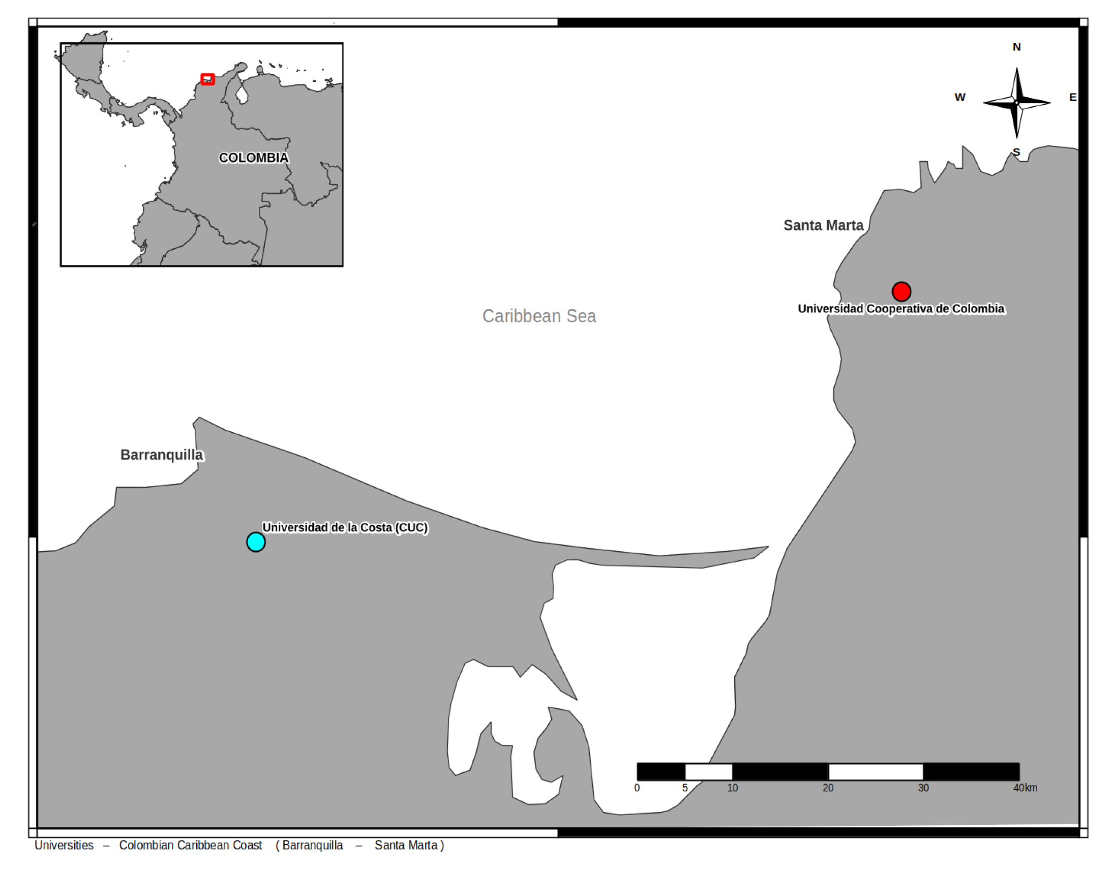
Figure 2.
Monitoring stations: (a) Located at Universidad de la Costa. (b) Located at Universidad Cooperativa de Colombia, Santa Marta Campus.
Figure 2.
Monitoring stations: (a) Located at Universidad de la Costa. (b) Located at Universidad Cooperativa de Colombia, Santa Marta Campus.
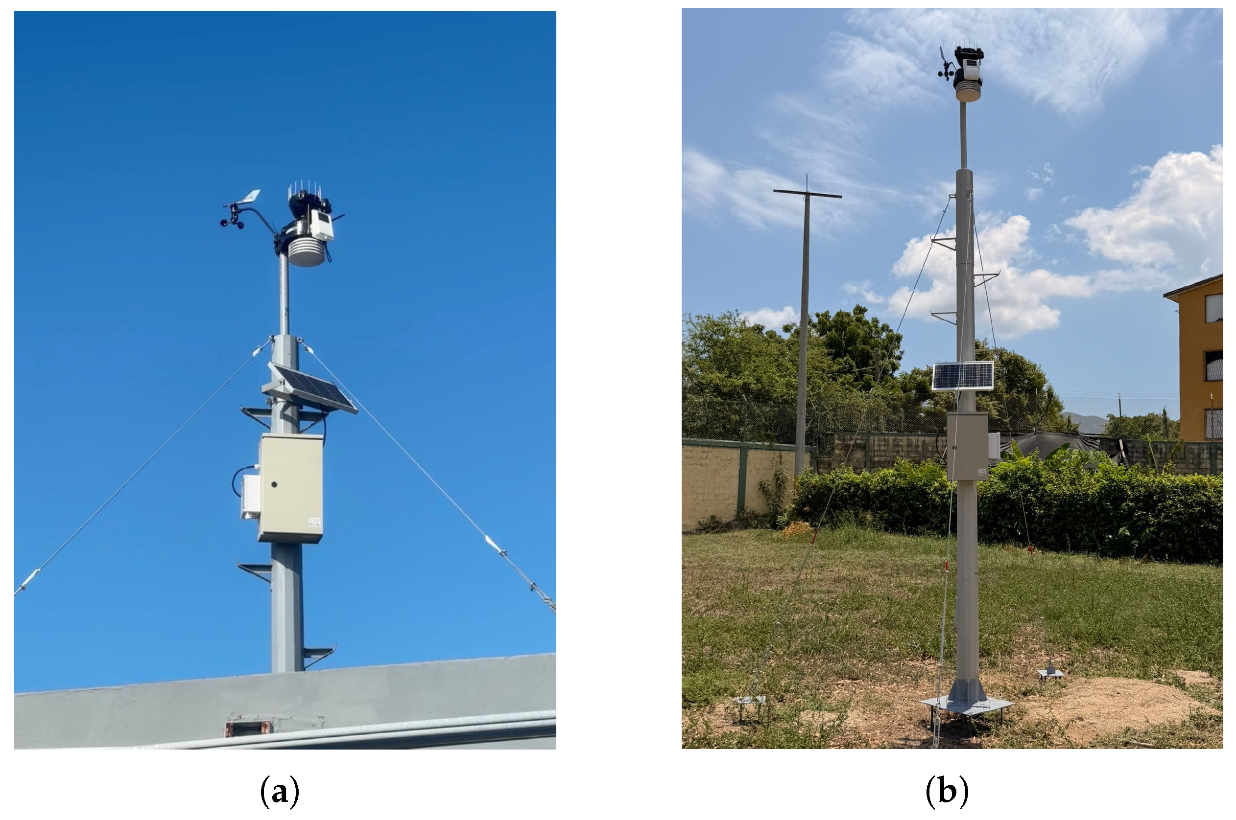
Figure 3.
Wind rose diagrams: (a) Station located at Universidad de la Costa. (b) Station located at Universidad Cooperativa de Colombia, Santa Marta Campus.
Figure 3.
Wind rose diagrams: (a) Station located at Universidad de la Costa. (b) Station located at Universidad Cooperativa de Colombia, Santa Marta Campus.
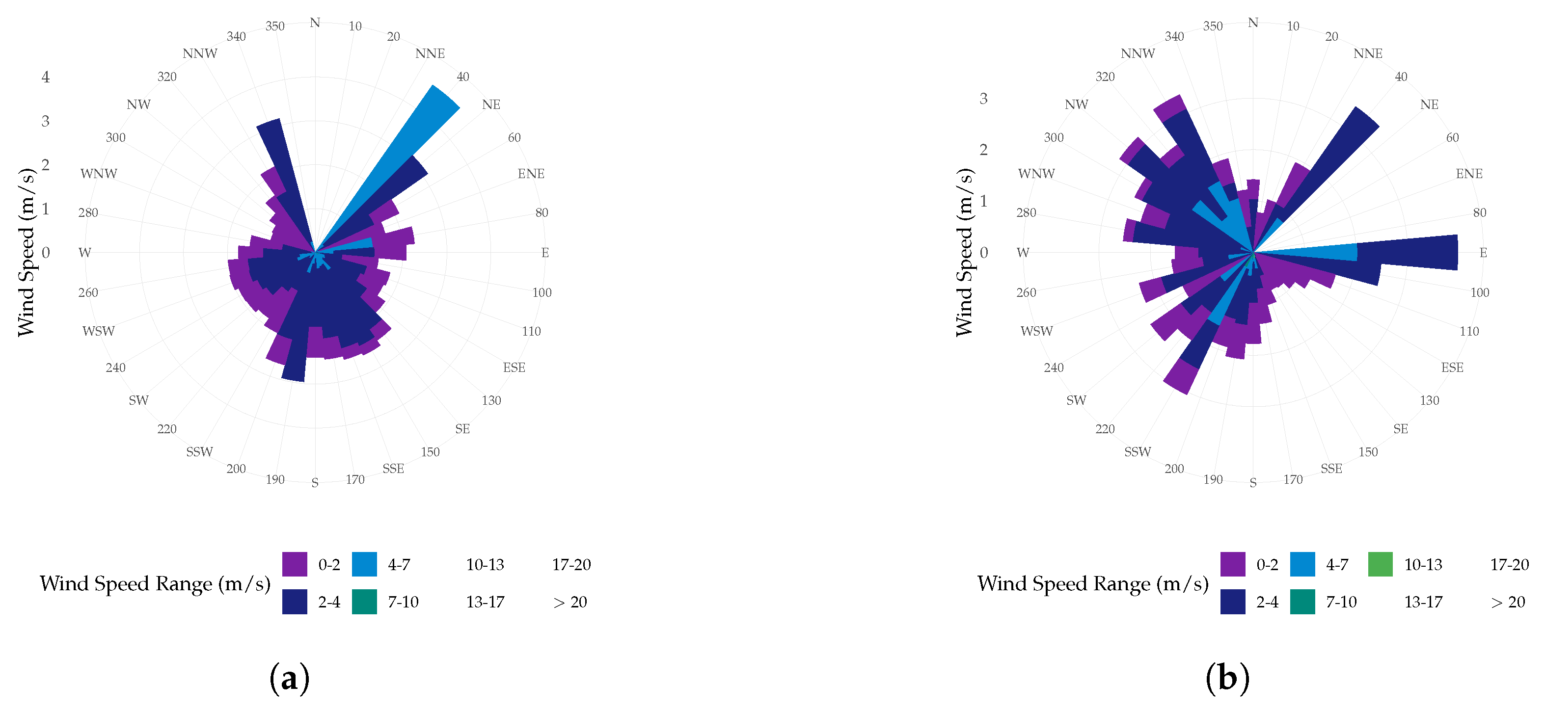
Figure 4.
Clean variables from the CUC station.
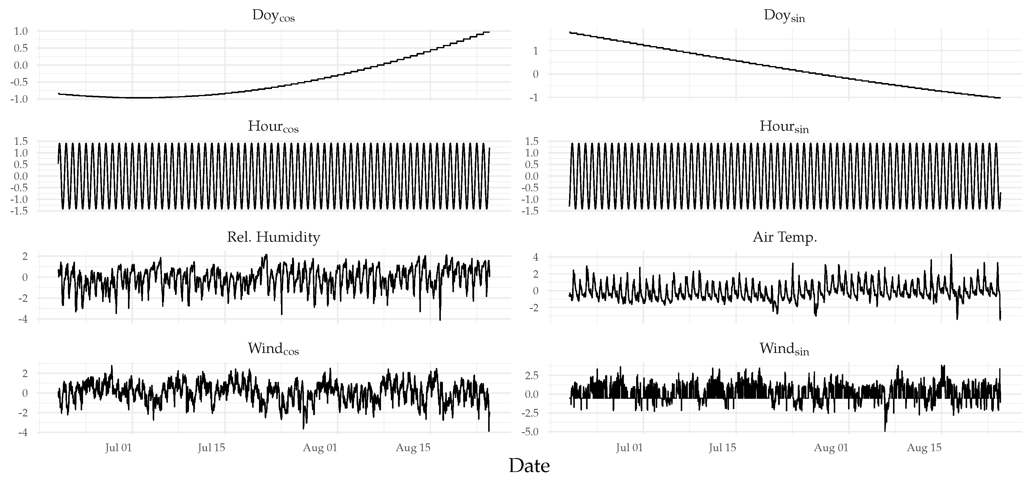
Figure 5.
Clean variables from the UCC station.
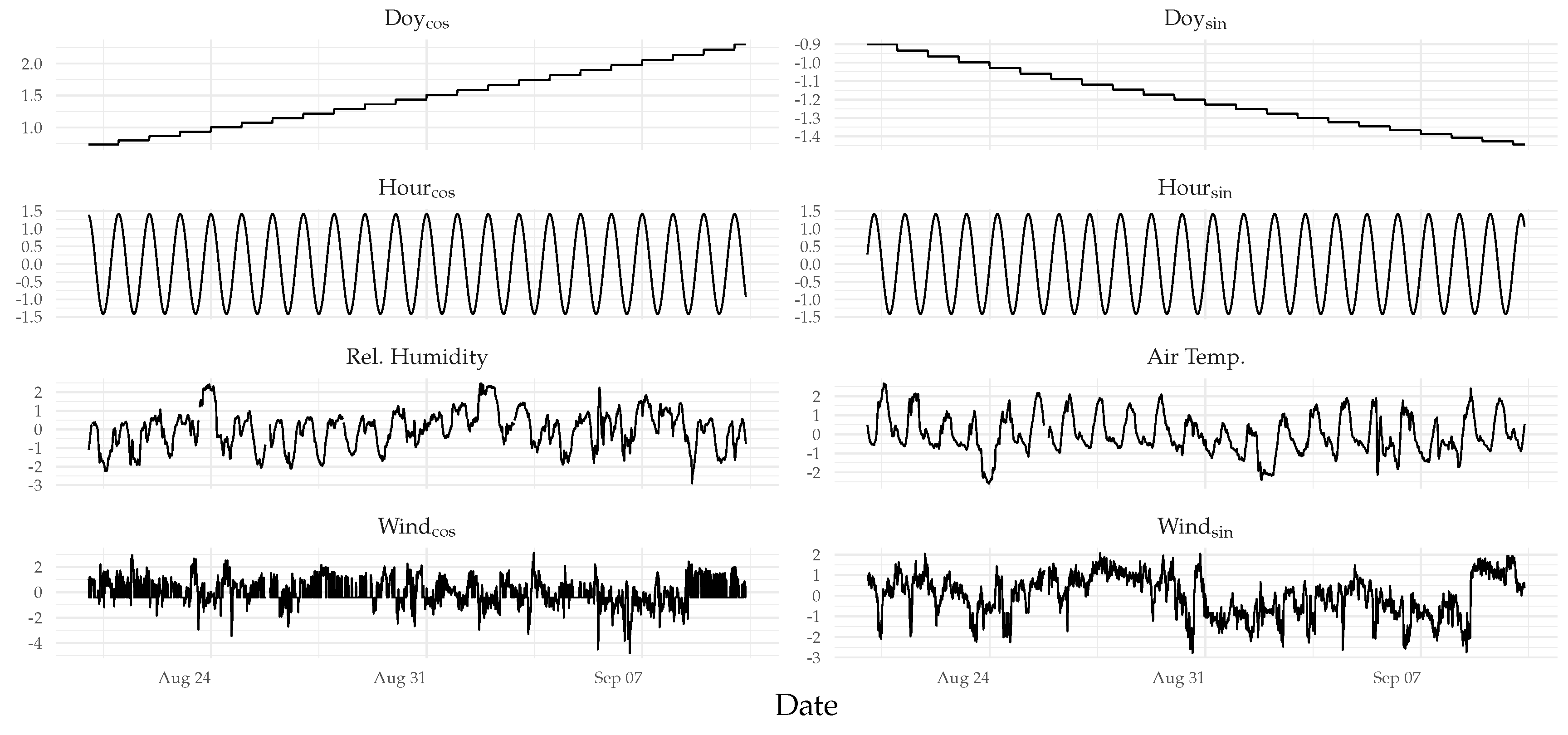
Figure 6.
Overview of imputation models.
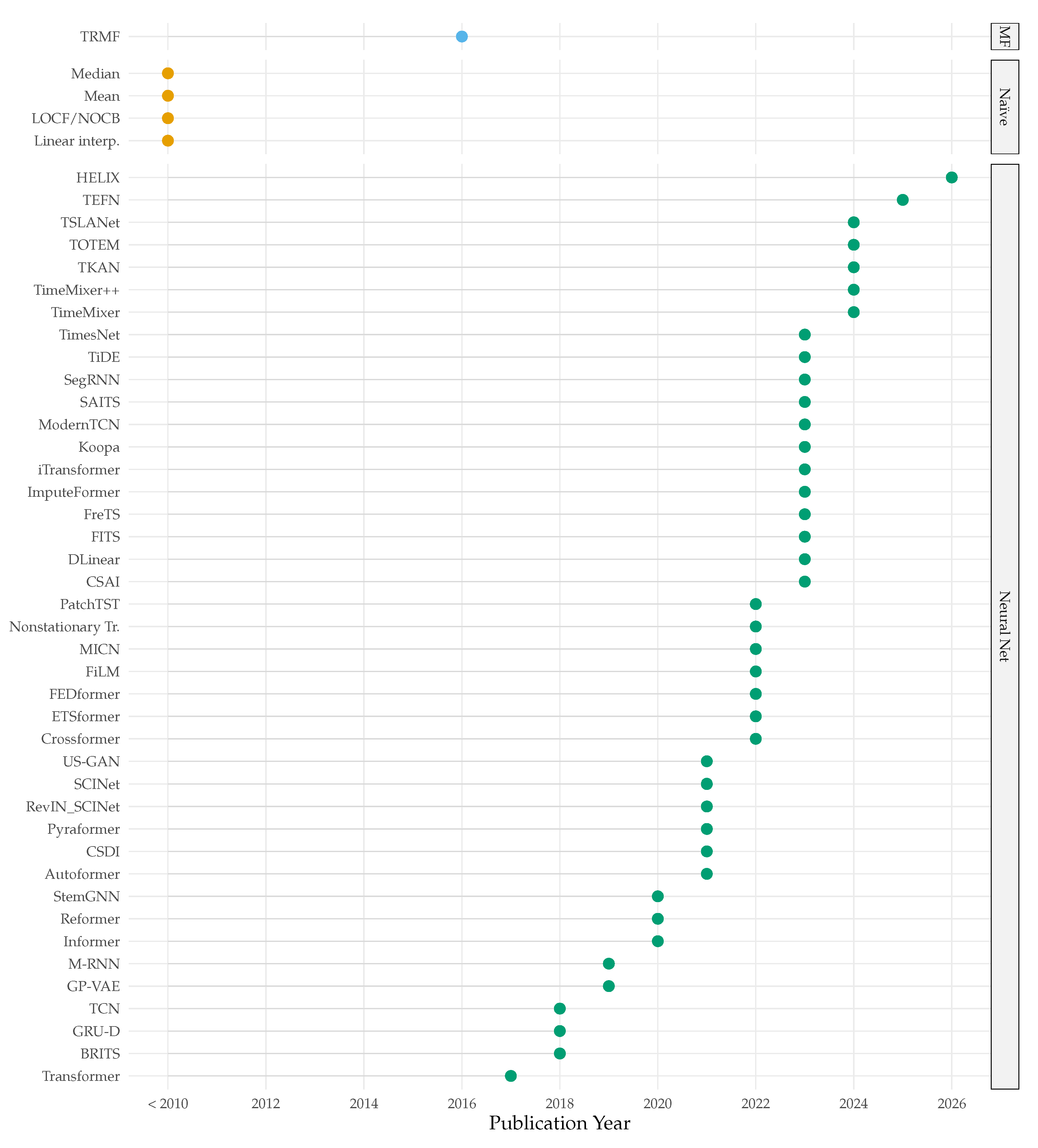
Figure 9.
Mean absolute error (z-score units) per target variable for the 15 best-ranked models (TOPSIS) at each station. Each row is labeled with the corresponding model name on the vertical axis, ordered from best (top) to worst (bottom) TOPSIS rank within its station.
Figure 9.
Mean absolute error (z-score units) per target variable for the 15 best-ranked models (TOPSIS) at each station. Each row is labeled with the corresponding model name on the vertical axis, ordered from best (top) to worst (bottom) TOPSIS rank within its station.
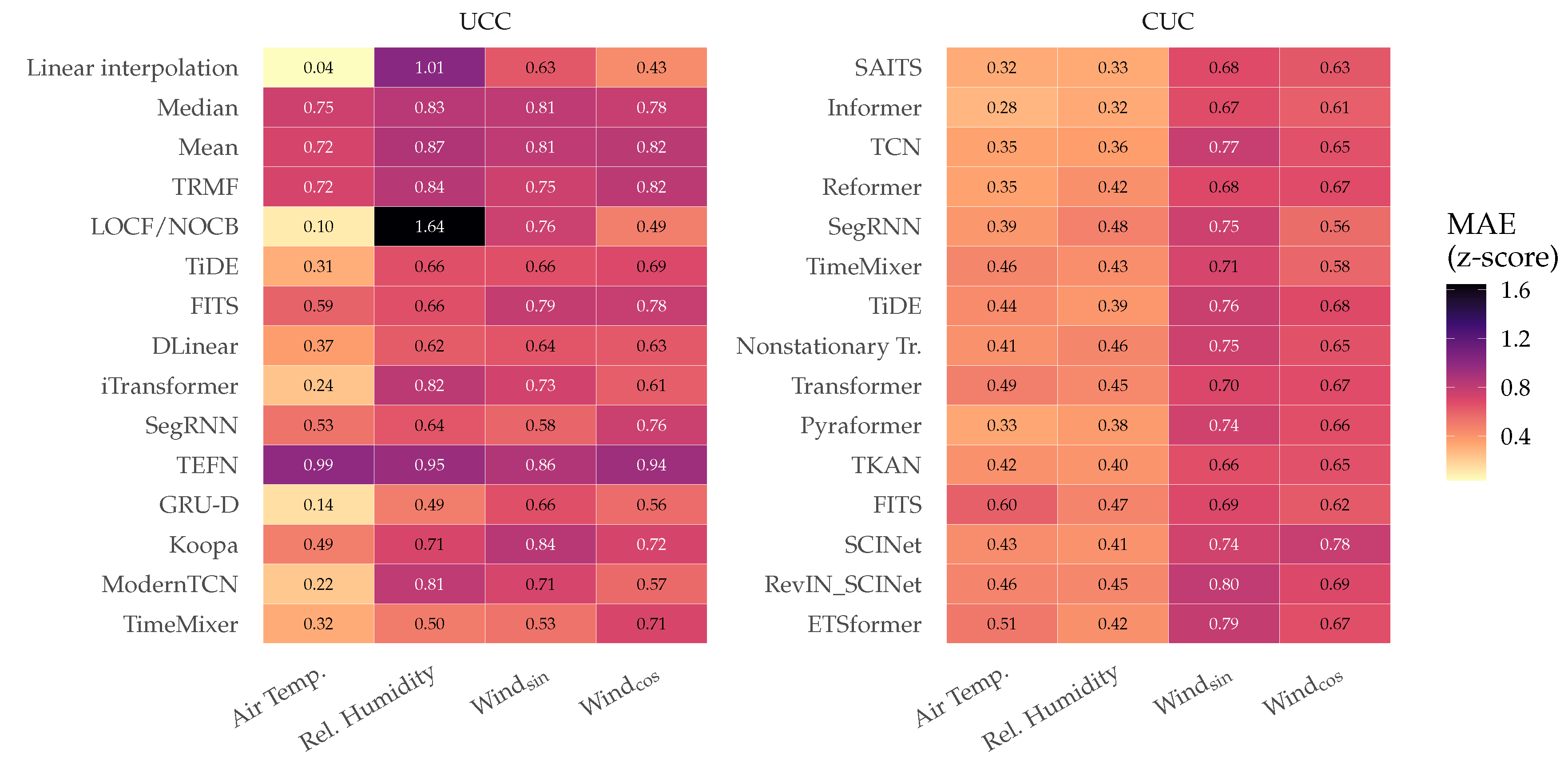
Figure 10.
Imputation accuracy (RMSE) versus total execution time (training plus inference, logarithmic axis). The dashed line joins the non-dominated (Pareto-efficient) models; models with RMSE are outside the plotted range.
Figure 10.
Imputation accuracy (RMSE) versus total execution time (training plus inference, logarithmic axis). The dashed line joins the non-dominated (Pareto-efficient) models; models with RMSE are outside the plotted range.
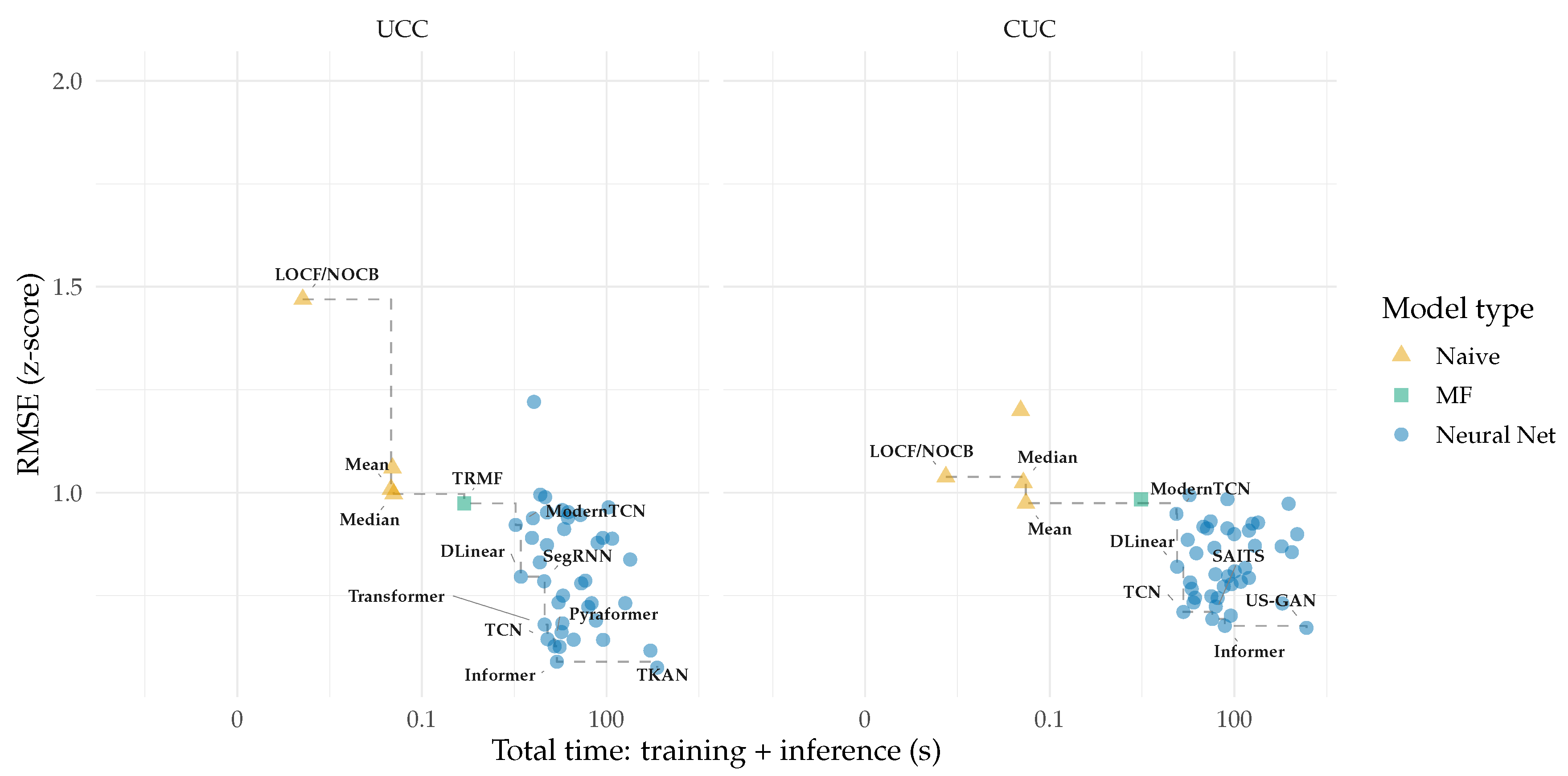
Figure 11.
Imputation accuracy (RMSE) versus average power consumption on the Jetson Orin Nano. The dashed line joins the non-dominated models; models with RMSE are outside the plotted range.
Figure 11.
Imputation accuracy (RMSE) versus average power consumption on the Jetson Orin Nano. The dashed line joins the non-dominated models; models with RMSE are outside the plotted range.
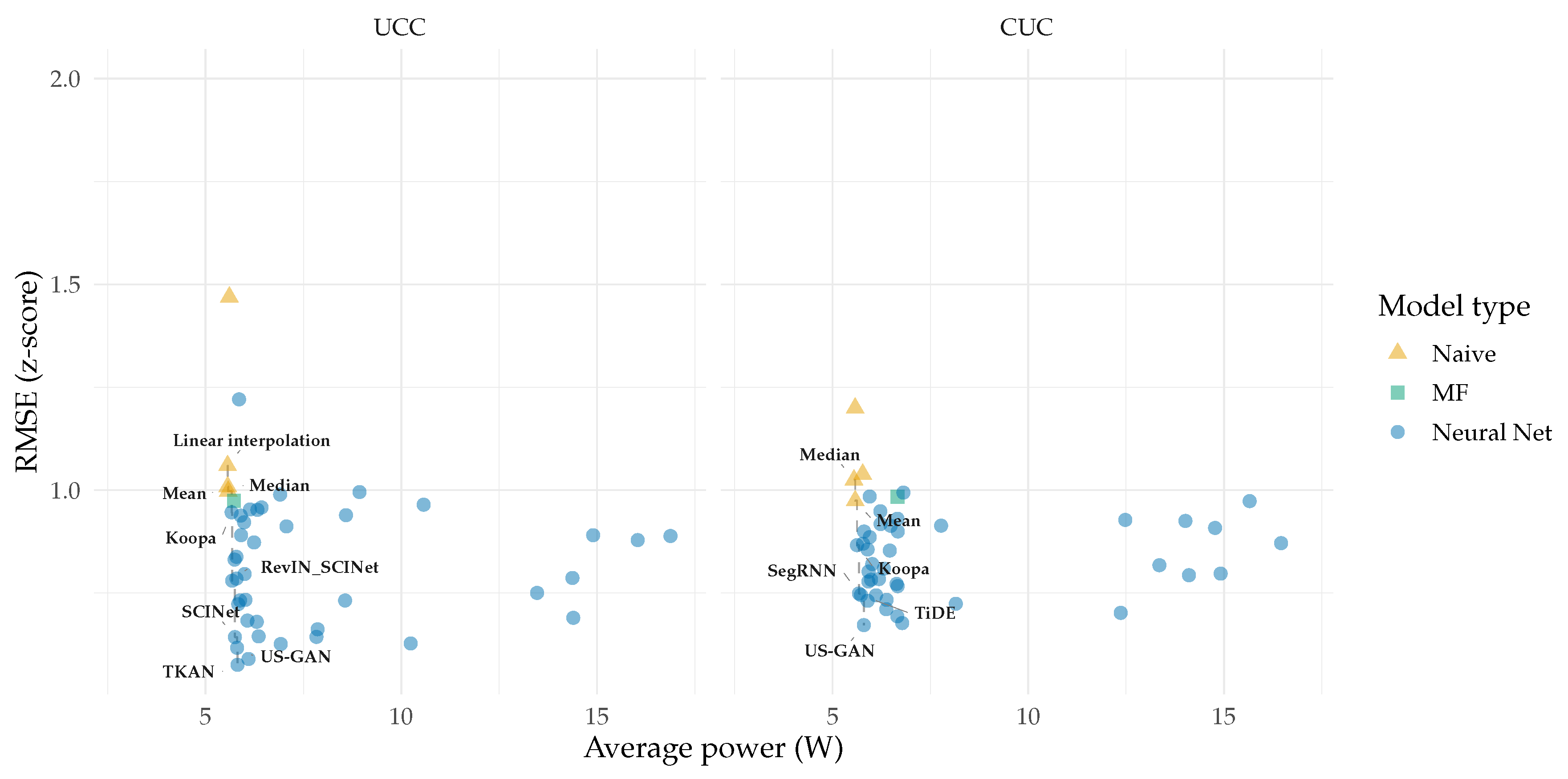
Figure 14.
Fifteen best alternatives according to TOPSIS, MARCOS and SPOTIS for the station-averaged decision matrix. Note that lower SPOTIS scores are better.
Figure 14.
Fifteen best alternatives according to TOPSIS, MARCOS and SPOTIS for the station-averaged decision matrix. Note that lower SPOTIS scores are better.
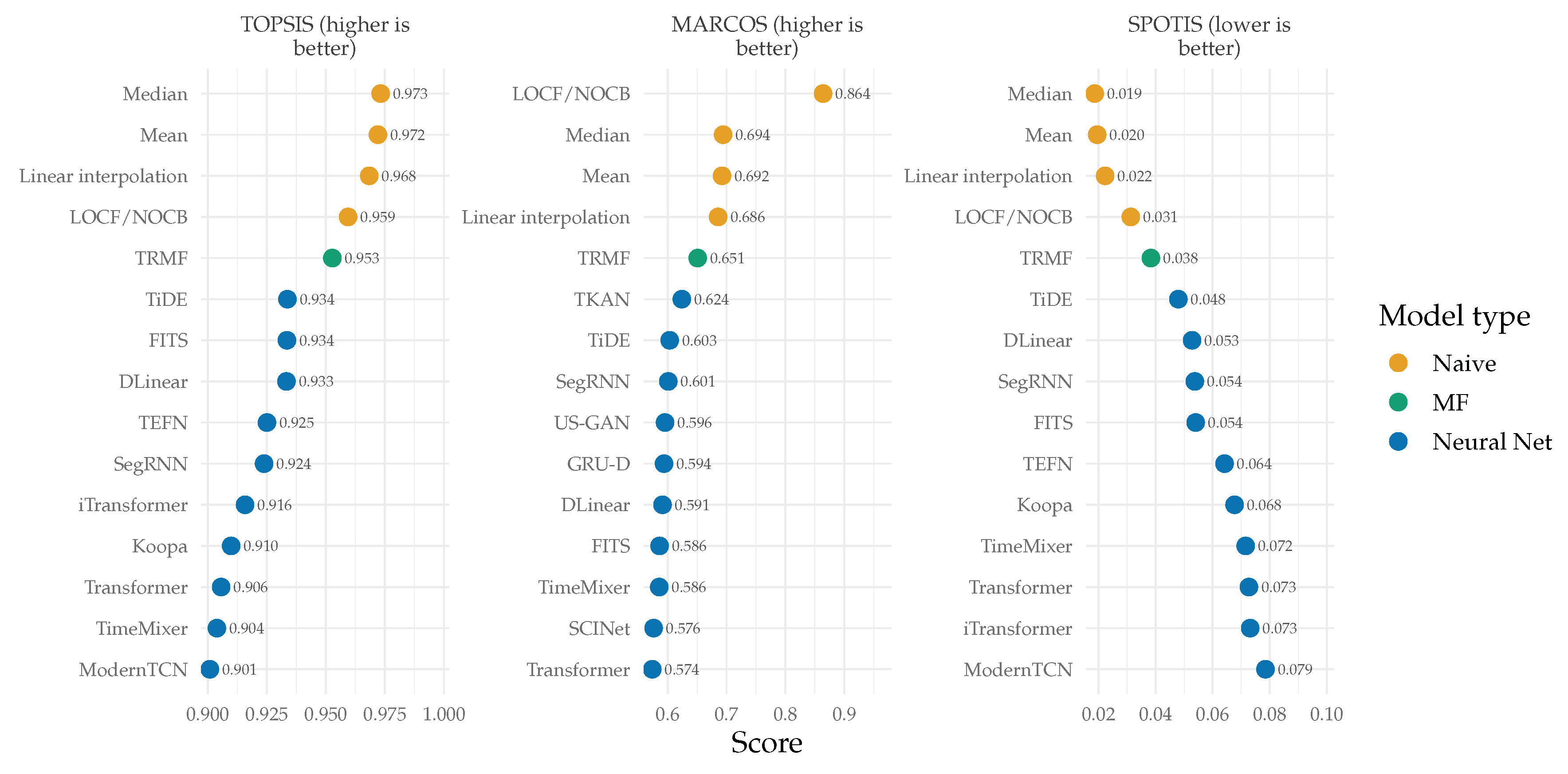
Figure 16.
Spearman rank correlation between the rankings produced by TOPSIS, MARCOS and SPOTIS.
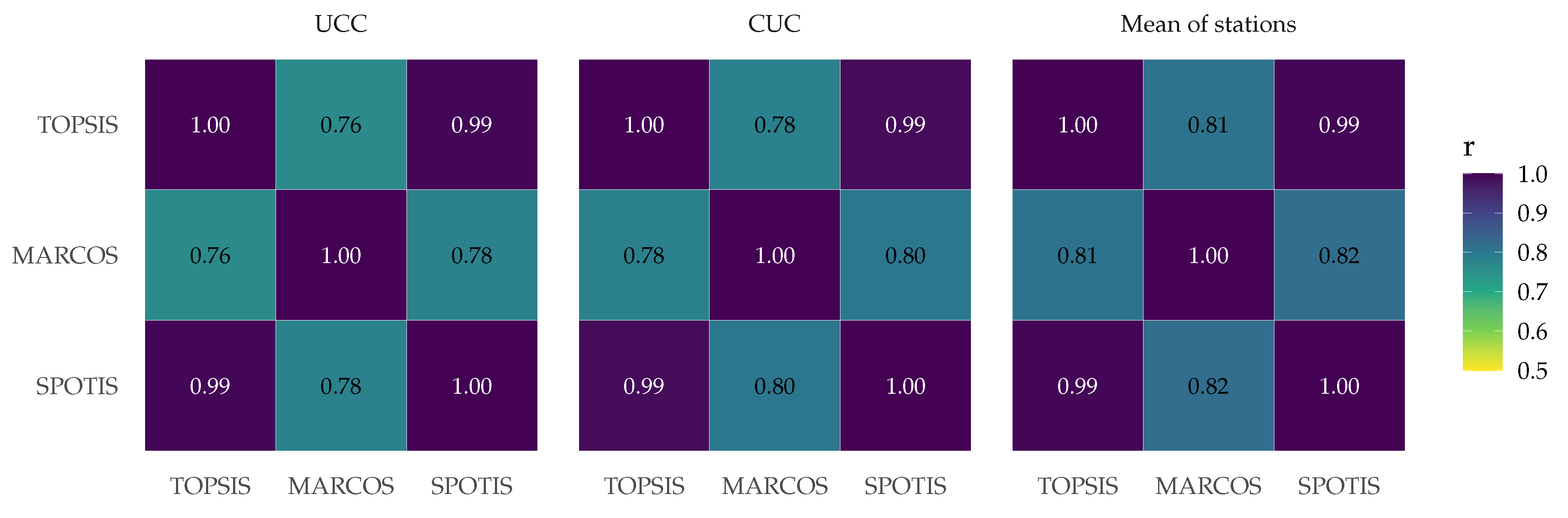
Figure 17.
Sensitivity of the rankings to the Entropy/CRITIC trade-off coefficient : Spearman correlation with the baseline ranking (, dashed line).
Figure 17.
Sensitivity of the rankings to the Entropy/CRITIC trade-off coefficient : Spearman correlation with the baseline ranking (, dashed line).
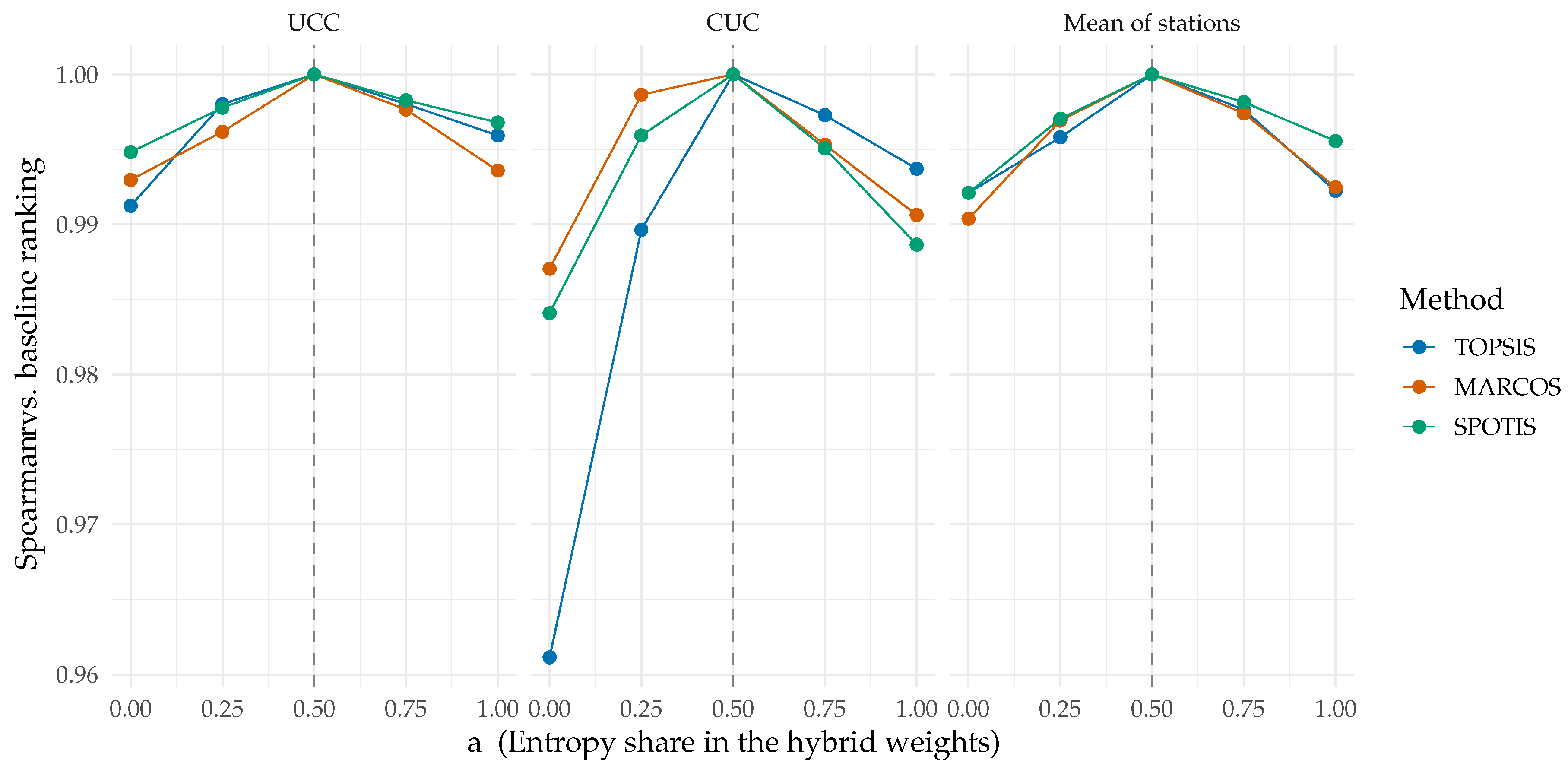
Figure 18.
Best-ranked model as a function of for each ranking method and station.
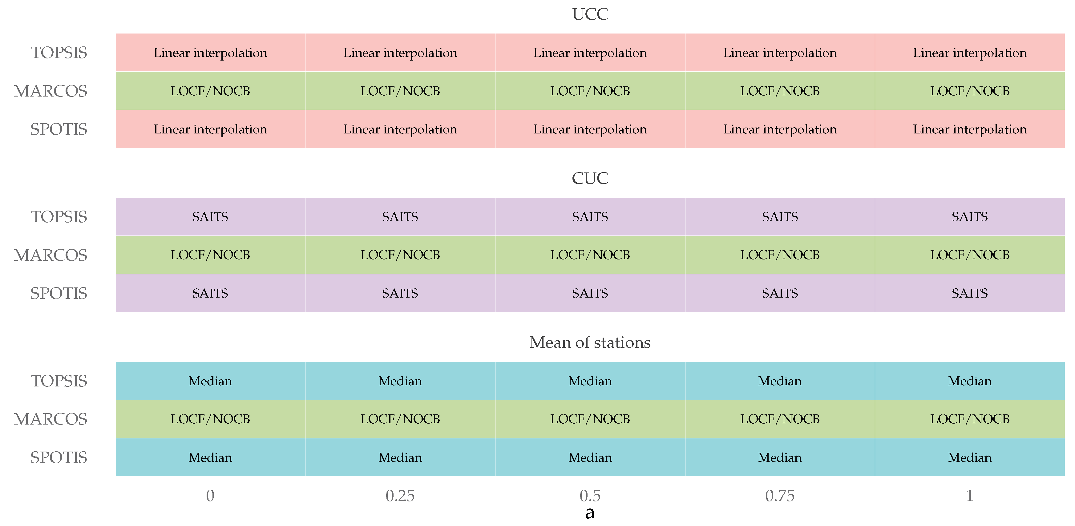
Figure 19.
Rank of each model at UCC versus rank at CUC for the three methods. The dashed line indicates identical ranks; is the Spearman correlation between stations.
Figure 19.
Rank of each model at UCC versus rank at CUC for the three methods. The dashed line indicates identical ranks; is the Spearman correlation between stations.
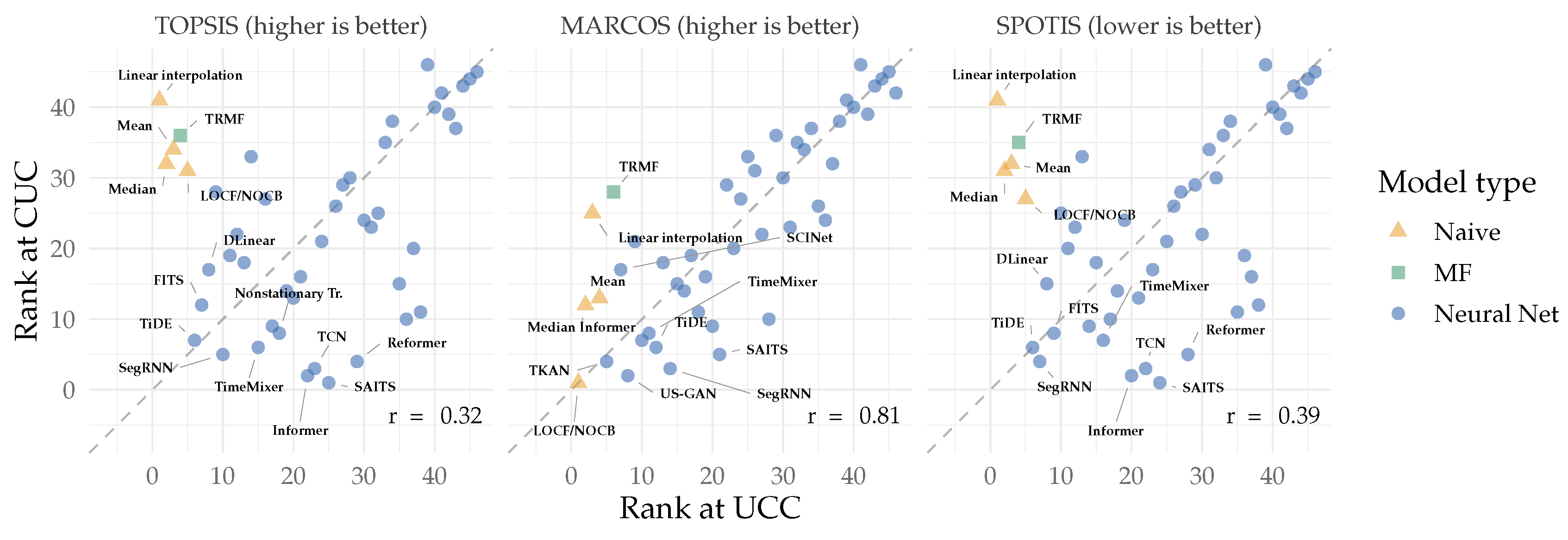
Table 1.
Technical specifications and operational features of the Davis Vantage Pro2 Wireless weather stations deployed at the two monitoring sites of this study (CUC and UCC).
Table 1.
Technical specifications and operational features of the Davis Vantage Pro2 Wireless weather stations deployed at the two monitoring sites of this study (CUC and UCC).
| Category | Parameter / Feature | Specification / Value |
|---|---|---|
| General Information | Manufacturer | Davis Instruments |
| Model / Part Number | Vantage Pro2 Wireless | |
| Data Transmission | Frequency-Hopping Spread Spectrum (FHSS) Wireless | |
| Range | Up to 300 m (1000 ft) line-of-sight | |
| Sensor Sampling | Wind Speed & Direction | Anemometer (2.5 s sampling interval) |
| Frequencies | Rainfall | Tipping bucket (20–24 s sampling interval) |
| Temperature | Silicon PN-junction / precision thermistor (10 s sampling interval) | |
| Relative Humidity | Solid-state capacitor (1 min sampling interval) | |
| Accuracy & Resolution | Wind Speed | m/s ( mph) or , whichever is greater |
| Wind Direction | ||
| Temperature | () | |
| Relative Humidity | ||
| Rainfall | 0.2 mm per tip (collection area: 214 ) | |
| Power & Operational | Operating Temperature | to |
| Environment | Primary Power Supply | 0.5 W Solar panel with supercapacitor storage |
| Radiation Shield | 24-Hour Active Solar-Powered Fan Aspirated Shield1 | |
| Backup Battery | 3V CR123A Lithium cell (autonomy years) | |
| Data Acquisition | Console Unit | WeatherLink Console (Part #6313, HD Touchscreen) |
| & Telemetry | Communication | Built-in Wi-Fi, direct Cloud / local database export |
1 Active 24-hour fan aspiration mitigates solar radiation bias, ensuring high-fidelity thermal and humidity measurements under intense solar irradiance.
Table 2.
Start and end dates of data recording across stations.
| Station | Start Date | End Date |
|---|---|---|
| CUC | 2026-06-17 15:45:00 | 2026-09-10 08:45:00 |
| UCC | 2026-06-20 09:15:00 | 2026-09-10 08:50:00 |
Table 3.
Statistical summary of the raw dataset for both stations.
| Station | Variable | N | Valid (n) | Min | Q1 | Median | Mean | Q3 | Max | Missing (n) | Missing (%) |
|---|---|---|---|---|---|---|---|---|---|---|---|
| CUC | Avg. Wind Speed | 8133 | 7847 | 286 | |||||||
| Avg. Wind Direction | 8133 | 7847 | 286 | ||||||||
| Rel. Humidity | 8133 | 7844 | 289 | ||||||||
| Air Temp. | 8133 | 7844 | 289 | ||||||||
| UCC | Avg. Wind Speed | 7871 | 2083 | 5788 | |||||||
| Avg. Wind Direction | 7871 | 2077 | 5794 | ||||||||
| Rel. Humidity | 7871 | 2073 | 5798 | ||||||||
| Air Temp. | 7871 | 2084 | 5787 |
Table 4.
Start and end dates of data recording across stations for the clean dataset.
| Station | Start Date | End Date |
|---|---|---|
| CUC | 2026-06-19 19:30:00 | 2026-08-23 22:00:00 |
| UCC | 2026-08-20 00:45:00 | 2026-09-10 08:45:00 |
Table 5.
NVIDIA Jetson Orin Nano hardware and software specifications.
| Feature | Specification |
|---|---|
| GPU | 1024-core NVIDIA Ampere, 32 Tensor Cores |
| CPU | 6-core Arm Cortex-A78AE v8.2 @ up to 1.73 GHz |
| Memory | 8 GB LPDDR5 (Unified Architecture) |
| Storage | NVMe SSD |
| Power Profile | 7–25 W (25 W / MAXN mode enabled) |
| Operating System | NVIDIA JetPack 6.2.3 (L4T R36.5.2, Ubuntu 22.04 LTS) |
| CUDA Toolkit | Version 12.6 (V12.6.68) |
Table 6.
Criteria structure and evaluation metrics for imputation models.
| Category | Criterion / Metric | Unit | Type | Description / Impact |
|---|---|---|---|---|
| Accuracy | MAE | z-score units | Cost | Mean absolute error over the artificially masked cells |
| RMSE | z-score units | Cost | Root mean square error over the artificially masked cells | |
| Comp. Overhead | Power | Watts (W) | Cost | Average board power on the Jetson Orin Nano during training and inference |
| RAM | Megabytes (MB) | Cost | Peak process memory plus reserved GPU memory (unified memory) | |
| Time | Seconds (s) | Cost | Training time plus latency of one full-series imputation call |
Table 9.
Decision criteria by model family for the station-averaged decision matrix: median (minimum–maximum). The single MF model (TRMF) is reported by its value. MAE and RMSE are expressed in z-score units.
Table 9.
Decision criteria by model family for the station-averaged decision matrix: median (minimum–maximum). The single MF model (TRMF) is reported by its value. MAE and RMSE are expressed in z-score units.
| Family | Models | MAE | RMSE | Power (W) | RAM (MB) | Time (s) |
|---|---|---|---|---|---|---|
| Naïve | 4 | 0.84 (0.80–0.95) | 1.07 (0.99–1.25) | 5.53 (5.51–5.63) | 605 (593–608) | 0.035 (0.002–0.036) |
| MF | 1 | 0.81 | 0.98 | 5.74 | 613 | 0.74 |
| Neural Net | 41 | 0.63 (0.48–3.83) | 0.81 (0.64–7.08) | 6.35 (5.63–15.6) | 1531 (1059–5791) | 34.5 (7.92–1015) |
Table 10.
Criteria weights. Entropy, CRITIC and hybrid weights () are given for each station and for the station-averaged matrix (Avg.).
Table 10.
Criteria weights. Entropy, CRITIC and hybrid weights () are given for each station and for the station-averaged matrix (Avg.).
| Entropy | CRITIC | Hybrid | |||||||
|---|---|---|---|---|---|---|---|---|---|
| Criterion | UCC | CUC | Avg. | UCC | CUC | Avg. | UCC | CUC | Avg. |
| MAE | 0.101 | 0.275 | 0.101 | 0.138 | 0.211 | 0.136 | 0.120 | 0.243 | 0.119 |
| RMSE | 0.100 | 0.096 | 0.099 | 0.138 | 0.139 | 0.136 | 0.119 | 0.117 | 0.118 |
| Power | 0.440 | 0.343 | 0.439 | 0.279 | 0.243 | 0.280 | 0.360 | 0.293 | 0.360 |
| RAM | 0.186 | 0.156 | 0.192 | 0.174 | 0.156 | 0.175 | 0.180 | 0.156 | 0.184 |
| Time | 0.172 | 0.129 | 0.168 | 0.271 | 0.252 | 0.272 | 0.221 | 0.190 | 0.220 |
Table 11.
Ten best alternatives according to TOPSIS for the station-averaged decision matrix. Criteria values are station averages (MAE and RMSE in z-score units); the scores of TOPSIS, MARCOS and SPOTIS are followed by the rank in parentheses (SPOTIS: lower score is better).
Table 11.
Ten best alternatives according to TOPSIS for the station-averaged decision matrix. Criteria values are station averages (MAE and RMSE in z-score units); the scores of TOPSIS, MARCOS and SPOTIS are followed by the rank in parentheses (SPOTIS: lower score is better).
| Model | Family | MAE | RMSE | Power (W) | RAM (MB) | Time (s) | TOPSIS | MARCOS | SPOTIS |
|---|---|---|---|---|---|---|---|---|---|
| Median | Naïve | 0.80 | 1.01 | 5.53 | 606 | 0.036 | 0.974 (1) | 0.678 (2) | 0.019 (1) |
| Mean | Naïve | 0.83 | 0.99 | 5.51 | 608 | 0.035 | 0.973 (2) | 0.678 (3) | 0.019 (2) |
| TRMF | MF | 0.81 | 0.98 | 5.74 | 613 | 0.74 | 0.969 (3) | 0.655 (5) | 0.027 (4) |
| Linear interpolation | Naïve | 0.85 | 1.13 | 5.53 | 605 | 0.035 | 0.969 (4) | 0.667 (4) | 0.023 (3) |
| LOCF/NOCB | Naïve | 0.95 | 1.25 | 5.63 | 593 | 0.0017 | 0.959 (5) | 0.855 (1) | 0.032 (5) |
| TiDE | Neural Net | 0.61 | 0.79 | 5.79 | 1091 | 14.4 | 0.957 (6) | 0.617 (8) | 0.038 (6) |
| iTransformer | Neural Net | 0.75 | 0.93 | 5.72 | 1111 | 15.9 | 0.954 (7) | 0.588 (17) | 0.044 (9) |
| FITS | Neural Net | 0.74 | 0.92 | 5.87 | 1060 | 8.00 | 0.953 (8) | 0.586 (19) | 0.045 (10) |
| DLinear | Neural Net | 0.62 | 0.81 | 5.97 | 1059 | 7.96 | 0.951 (9) | 0.606 (11) | 0.043 (8) |
| SegRNN | Neural Net | 0.63 | 0.83 | 5.74 | 1209 | 13.2 | 0.951 (10) | 0.602 (12) | 0.042 (7) |
Table 12.
Five best alternatives according to TOPSIS at each station. Format as in Table 11.
Table 12.
Five best alternatives according to TOPSIS at each station. Format as in Table 11.
| Station | Model | MAE | RMSE | Power (W) | RAM (MB) | Time (s) | TOPSIS | MARCOS | SPOTIS |
|---|---|---|---|---|---|---|---|---|---|
| UCC | Linear interp. | 0.80 | 1.06 | 5.49 | 604 | 0.032 | 0.984 (1) | 0.667 (4) | 0.012 (1) |
| Median | 0.82 | 1.00 | 5.51 | 600 | 0.037 | 0.984 (2) | 0.668 (2) | 0.012 (3) | |
| Mean | 0.84 | 1.01 | 5.48 | 606 | 0.031 | 0.983 (3) | 0.668 (3) | 0.012 (2) | |
| TRMF | 0.80 | 0.97 | 5.67 | 610 | 0.49 | 0.980 (4) | 0.653 (6) | 0.018 (4) | |
| LOCF/NOCB | 1.16 | 1.47 | 5.54 | 593 | 0.0012 | 0.967 (5) | 0.836 (1) | 0.024 (5) | |
| CUC | SCINet | 0.49 | 0.70 | 5.80 | 1594 | 89.7 | 0.929 (1) | 0.652 (2) | 0.054 (1) |
| TimeMixer | 0.54 | 0.74 | 6.10 | 1290 | 52.2 | 0.920 (2) | 0.626 (9) | 0.076 (4) | |
| TiDE | 0.57 | 0.74 | 5.70 | 1094 | 22.5 | 0.915 (3) | 0.646 (5) | 0.067 (2) | |
| SegRNN | 0.57 | 0.77 | 5.70 | 1206 | 20.6 | 0.907 (4) | 0.634 (8) | 0.074 (3) | |
| TCN | 0.56 | 0.73 | 6.16 | 1341 | 19.6 | 0.906 (5) | 0.617 (12) | 0.082 (6) |
Disclaimer/Publisher’s Note: The statements, opinions and data contained in all publications are solely those of the individual author(s) and contributor(s) and not of MDPI and/or the editor(s). MDPI and/or the editor(s) disclaim responsibility for any injury to people or property resulting from any ideas, methods, instructions or products referred to in the content. |
© 2026 by the authors. Licensee MDPI, Basel, Switzerland. This article is an open access article distributed under the terms and conditions of the Creative Commons Attribution (CC BY) license (http://creativecommons.org/licenses/by/4.0/).
Copyright: This open access article is published under a Creative Commons CC BY 4.0 license, which permit the free download, distribution, and reuse, provided that the author and preprint are cited in any reuse.