
Submitted:
30 September 2026
Posted:
01 October 2026
You are already at the latest version
Abstract
The concept of tangent spaces that is utilized in physics to analyze geometric structure and motion in a smooth manifold are applied to finite simple connected graphs. This note develops the incidence structure of a graph that represents the tangent structure of a graph, develops vertex incidence spaces that are vector spaces at each vertex consisting of vectors tangent to that vertex, and reveals the connection operator of a graph. From the graph tangent structure perspective, an example of communication and information flow in a collaboration network that utilizes parallel transport is discussed along with a discussion of additional graph dimensions. Several concepts are left to this note's readers for further development such as possible tangent structure polynomials based on vertex degree and a possible application to knot theory. As with any new perspective, the full realm of applications is in the future.
Keywords:
graphic tangent spaces
; graphic connection operator
; graph dimension
; degree projection
MSC: Primary 05C99
1. Introduction
The concept of tangent structure is utilized in physics for analyzing the geometry and motion in smooth curved manifolds. Borrowing tangency concepts from physics, this note shows that each edge in a finite simple connected graph can be viewed as a connection between tangent spaces with tangent vectors at each vertex. This viewpoint provides greater foundation and expanded understanding of graph structure, plus increasing the potential of various research areas to gain from the simplicity inherent in graphs depicting networks. Graph tangent structure is a new perspective on material that dates back to the origins of graph theory. In his 1948 article [11] that gave a third viewpoint for non-relativistic quantum mechanics, Richard Feynman stated “... There are, therefore, no fundamentally new results [in his article]. However, there is a pleasure in recognizing old things from a new point of view." Feynman’s way of taking accepted ideas, and visualizing them in a different manner, lead to his innovation of Feynman diagrams and QED.
Imagine particle , identified with a vector, moving on the “surface" created by a finite set of vertices, that are defined on basis vectors, in edgeless graph G. Allow ’s movements to generate edges as determined by G’s incidence relationship function, , that might be a piece of code. Based on ’s instructions, vector leaves initial vertex along a trajectory that is tangent to and begins to travel to the next vertex, as dictated by . Vertices and are orthogonal to each other, so as approaches , the particle’s trajectory needs to become tangent to . By its definition, graphic connection operator changes ’s initial movement that is tangent to , to be tangent to , allowing to arrive at . This is the story of parallel transport of a vector in simple connected G.
For any new approach, the best way to begin is by examining the simplest possible situation first. This note discusses simple connected graphs G defined on the binary field, in flat space.
As discussed in Section 2, concepts relating to tangency range from common usage in comparing ideas, to vectors at points on smooth manifolds. In this note, the phrase “incidence" is often utilized in place of “tangent", with a goal of avoiding the implication that all G are manifolds. The incidence space of G is a function space, that is analogous to the tangent bundle, of G that forms the incidence graph, as discussed in Section 3. Because this note might have a wide range of readers, a few basic graph concepts are also given in Section 3. Proposition 1 states that edges that share a vertex are tangent to each other at , and edges that share no end vertex are orthogonal to each other. Any vertex is tangent to its incident edges and that vertex is orthogonal to non-incident edges as given by Proposition 2. Open edges are defined that have both tangent and orthogonal aspects. Utilizing the concept of open edges and maps, Proposition 3 says that any vertex is tangent to its set of incident open edges and orthogonal to non-incident open edges. Open edges that share a vertex are tangent to each other by Proposition 4, while Proposition 5 states that open edges that are not incident to a vertex are orthogonal. Theorem 1 compares the tangent structure of open and closed edges in graph G. Section 3 concludes with the connection operator of a graph and parallel transport that apply to flat space, plus a simple visualization of graphic tangent structure.
Because this note provides a new way to conceptualize the vector spaces of a simple connected graph, a few applications are given in Section 4. Have you ever had a conversation where you felt that everything you said was orthogonal to the other person? This experience is discussed in connection to the information flow in a collaboration network. Also discussed in Section 4 are new perspectives on graph dimension where Theorem 2 refers to the incidence dimension, and the elemental dimension, of any finite simple connected graph. With further investigation and proof left to the readers of this note, the vertex polynomial, as given in [2], might apply to the tangent structure of a graph. Section 4 concludes with a possible application to knot theory. Although not discussed in this note, possible applications may be found in quantum computing.
The fact that graphs have vector spaces is utilized throughout this note. Although specifics are difficult to pinpoint, it appears that graph vector spaces were first introduced in the mid to late 1800s, with a more recent discussion in [14] dated 1958. The incidence graph of a graph, reflects a graph’s tangent structure. Based on finite geometric structures, so not based on graphs, F.W. Levi introduced the concept of the incidence graph in his 1942 article [18]. Although graphs have several polynomials, in 2023 [2], H. Ahmed, et al introduced the vertex degree polynomial of a graph. The application of the vertex degree polynomial to the tangent structure of graphs is left to this note’s readers. As any reader of this note will discover, the concepts presented here are new and also date to the origin of graph theory by Leonhard Euler with respect to the Königsberg bridges [9,24].
2. Tangency
With respect to an idea, common usage of the word “tangent" in a discussion means that the particular tangent idea is aligned with other ideas to which it is being compared. In other words, if two ideas go in a similar direction, then the ideas are tangent to each other.
A general physics concept of a tangent vector is taken directly from [5]:“The speed [along a curve] will be relative to the speed of other curves having the same direction. The notion of the tangent vector or velocity vector of a curve at a point is exactly this combination of direction and speed." With respect to a smooth manifold, the material covered in this subsection is fairly general with more specific information given in [5,15,23].
A smooth manifold is a surface that is locally Euclidean. In other words, Euclidean space is found at each point on the manifold although the entire manifold may not be Euclidean. Therefore, a manifold is not necessarily a vector space, although vector spaces exist in the neighborhood of each point.
The concept of a tangent space , at a point p on a smooth manifold M, is a vector space containing vectors tangent to the specific point p. The dimension of a tangent space is that of manifold M. With respect to a manifold, the union of tangent spaces is called the tangent bundle which is itself a manifold. For a d-dimensional manifold, the dimension of the tangent bundle manifold is [5]. Various aspects of M can be utilized to define the tangent spaces, one of which considers each tangent vector as a velocity vector of a moving particle that touches M at p. The vector space at p, that is the tangent space at p, is then the collection of all such velocity vectors at point p.
How could these manifold concepts apply to a graph? There are well known connections between graphs and manifolds as given by the following example. Consider the hypercube graph generally known by its geometric name: “a cube". Although a cube is not a differentiable surface due to its sharp points, it is well recognized that, from a topological perspective, a cube can be transformed into a sphere where the surface is a smooth manifold. This is just one example of a graph that relates to a manifold. Various mathematical areas link graphs to other algebraic structures that can be manifolds based on the existence of certain conditions in the graphs. However, not all graphs relate to manifolds. The tangent structure of a graph in this note is adapted to the graph discrete structure, and applies to all simple connected graphs defined on . Because the use of “tangent" implies the existence of a manifold, and not all graphs relate to manifolds, this note also uses “incidence vector", “vertex incidence space" () and “graph incidence space" (or simply incidence space) that are analogous to a manifold’s tangent vector, to the manifold’s tangent space and to the manifold’s tangent bundle, respectively. Consider the idea of a velocity vector at a manifold point described at the beginning of this subsection. In a graph, the speed can be considered to be 1 with direction defined on as either orthogonal, or not, by the use of inner product of vectors.
3. Incidence Structure That Is the Tangent Structure of a Graph
It is assumed that any reader of this note has some familiarity with graph theory and linear algebra. A concise but quite complete coverage of graph theory and linear algebra (plus group theory) is in [3]’s “Introduction".
Regarding notation, in this note, “:=" is used for the phrase “is defined as" or “is defined by". The most common notation for a graph G is where V is the vertex set of G and E is G’s edge set. Using this notation assumes that anyone viewing the notation recognizes that there also exists, in any graph, the incidence relationship defining the edges in E as connections between the vertices in V. In other words, for all G, the existence of edges in G is completely determined by the incidence relationship that is a well-defined function, or set of functions. This includes graphs with randomly generated edges and all edgeless graphs. Therefore, graph G here is where I denotes the set of incidence relationships of G. Set I is given greater clarity and precision throughout this note. Because this note discusses several related graphs, when specificity is required, the vertex set of G is denoted with order , G’s edge set with size , and is the set of incidence relationships in G. When referring to general graph order and size, n is order and m is size, and the cardinality of set X is . It is important to keep in mind that a graph is simply a visual image, or a diagram, of vector spaces formed from a set of objects and the relationships between the objects.
Vertices and joined by an edge are adjacent to each other, denoted , and edge joining vertices and is incident to and that are called the edge’s end vertices. In this note, two sets of related edges are discussed, closed edges and open edges. Defined by their end vertices , let indicate a closed edge in G. A pair of closed edges that share the same end vertex are referred to as edge-adjacent.
Open edge is a vertex-less edge related to vertex , and, in simple loopless G, there exist open edges for each vertex in . Focusing on greater specificity, denote the incidence relationship definition as and let be the set of that use with respect to distinct specific to generate, or not generate, edge where . Let be an assignment of to a specific indicating that is true for with respect to vertex . In other words, from the possible for any in G, not necessarily all result in an map to . Call those that result in realized open edges. Our concern in this note is with the realized open edges. Thus, unless otherwise specified, let here indicate a realized open edge where is the set of all realized open edges.
As explained later, index i reflects that is tangent to but orthogonal to as reflected by index j in , with G defined on . This notation is depicted in Figure 1. The choice of index placement is based on the notation used for tensors, with possible further development of the tensor-like structure in G left to the readers of this note. When all vertex pairs have been compared based on , all open become by the use of as discussed in Section 3.7 covering connection and parallel transport.
Perhaps the best way to visualize the incidence process is with respect to software code. The number of either closed edges, or the number of realized , incident to any vertex v is v’s degree, denoted by . Let a coded function be designed to determine the appropriateness of generating an edge adjacent to a specific vertex. Then, by the definition of , let the piece of code be for a specific G. The set is the set of actual executions of the code where each is an iteration for one specific vertex . As algebraic structures, all G have this set of relationships. Let be defined on binary field where is an incidence relationship regarding a particular vertex with respect to . If an is defined to generate at , then ; otherwise, . Thus, out of the possible , only have and form maps . Once all iterations are complete, by the use of , each and are connected to form making complete in undirected G. Thus, each results from two generating and assignments; so set of closed edges is the result of a completed set of iterations that represent , the originating code, that is the graph definition. Let be a function that connects and maps. So each can be identified to a specific , allowing each to represent in . Thus, in this note, let indicate . Any incidence relationship in this note is defined to only generate undirected edges. Note that the sum of all vertex degrees in G is where all are realized.
Following are a few graph theory concepts that can be skipped (typical notation is used) by those familiar with graph theory. A complete graph is a graph on n vertices where every vertex pair in is adjacent. Let denote the cardinality of set X. A bipartite graph, can have its vertex set partitioned into subsets X and Y whose union is the vertex set V that has cardinality with and . In , closed edges exist only between members of X and Y with no edges between the members of each vertex subset. A cycle graph is a set of n vertices all of which compose a cycle resulting in all vertices having . A tree is an acyclic graph, and when a tree has only a single limb and no branches (all vertices form a straight line), the tree is a path graph, . A planar graph is G that can be embedded in the Euclidean plane. Random graphs have edges, and possibly vertices, defined on probability functions. An empty graph is a graph with n number of vertices but no edges, and a null graph has no vertices (so no edges). There exist many other graph families and additional information can be found in [7]. An induced subgraph of G consists of a vertex subset that forms a subgraph in G where vertices adjacent in S are also adjacent in G. Graph G is connected if there exists a sequence of edges and their incident vertices where no vertices or edges are repeated between all vertex pairs in G. Although G in this note is considered to have a single connected component (unless specified otherwise), a connected component (called component for short) of G is a maximal connected subgraph of G. Later in this note, graphs that may have multiple components are defined with respect to G.
3.1. Vector Spaces of a Graph
A vector in this note is denoted either as or as that is the transpose of a column vector. Typical standard basis vector notation is used, so in 4 dimensions is . The intersection of two vector spaces is a vector space, but the union of two vector spaces is usually not a vector space. Instead, two vector spaces can be summed to form a vector space. Symmetric difference is a summation of two sets of objects that excludes the intersection of the two sets. In other words, for two vector spaces X and Y, their symmetric difference is that forms a vector space. It is well known that any power set of a set forms a vector space.
Define G on the binary field of elements . With G over , it is well accepted that both the vertex set and closed edge set of G form vector spaces [3,4,9,14,24]. The vertex space of any graph is defined by with a dimension given by , while the edge space of G, defined by , has dimension . In the above sources, the edges in are the closed edges , identified by , that are defined to contain end vertices.
3.2. Three Matrices of a Graph
An example simple connected G is displayed on the left in Figure 2. The incidence matrix of G, , is a positive binary matrix with rows indexed by and columns indexed by . In other words, maps to . Typically, is not square. Element equals 1 when vertex (i ranges over n) is incident to edge where j ranges over m. The matrix shown in the left center of Figure 2 is the example G’s .
There is another way to view the matrix of G. Label the vertex set of G with positive integers, and label each closed edge, or , as a combination of the edge’s end vertices. The example G in Figure 2 has this labeling. Now assign the standard basis vectors to the vertices in G based on numerical vertex order, so vertex 0 in the example G is , whose transpose is . Define each closed edge, vector, or , in G as the sum of the vertex vectors for the edge’s end vertices. Working with vector transposes, for the example G, this results in edge 03 having vector . Placing these edge vectors as columns in a matrix with row indices from ordered so that the end vertices of each edge align with the 1s in the column edge vectors. This matrix is that reflects the incidence relationships of G with respect to the standard basis.
The adjacency matrix of G, , is a positive symmetric binary matrix indexed by where is 1 when vertex in G, and zero otherwise. is a linear mapping of to . For the example G in Figure 2, G’s is in the right center.
The set of vertices adjacent to v is the open neighborhood of v denoted . The common neighbor matrix, CNM, is a symmetric matrix with indices defined on where element CNM, at the intersection of row and column , is the number of common neighbors that shares with . A zero valued reflects that the intersection of the neighborhoods is empty. Any CNM can be defined to include the common neighbors of vertices that are adjacent and/or those that are not adjacent. Thus, for nonadjacent and , . The CNM based on nonadjacent vertices for any is an all zero matrix because all vertex pairs are adjacent creating empty nonadjacent intersections. For nonadjacent vertices, if G is bipartite and is non-zero, then and are in the same bipartite set. The CNM for nonadjacent vertices in the example G is on the right of Figure 2. Because only vertices 1 and 3 are nonadjacent, most of the have zeroes; but vertices 1 and 3 share two neighbors, 0 and 2.
3.3. Orthogonality in a Graph
Because this note is focused on the tangent structure of G, and tangency implies direction, how do the vertices and edges of G relate to each other with respect to direction in G? If an inner product of two distinct vectors in equals 0, then the two vectors are orthogonal. Thus, for vectors in , if the inner product of two distinct vectors equals 1, then the two vectors are going in a similar direction; so here these two vectors are considered to be tangent to each other in .
Let each be represented by , and let vertices be identified with . For any G over , in matrix , if any column vector pair has an inner product equaling zero, then these two closed edges (or two ), represented by the column vectors, are orthogonal. However, if the inner product equals 1 then the two column vectors go in a similar direction, so they have a tangent relationship. For the example G in Figure 2, edges 01 and 23 are orthogonal, as are edges 12 and 03. Because neither of these edge pairs share end vertices, the 1s in their columns align with zero making the inner product a zero sum. This is true for all columns representing edges that do not share any end vertices in G. Now examine the columns for edges 01 and 12 that share vertex 1 as an end vertex. An inner product of these two column vectors results in 1 because the row indexed by shared vertex 1 aligns two 1s. Again, this situation is true for any column pair representing edge-adjacent edges in any G. This proves Proposition 1.
Proposition 1.
Suppose G is simple and connected, defined on , with vertices as standard basis vectors and each closed edge () as the sum of the end vertices’ vectors. Then edge-adjacent in G are tangent to each other in G, and that are not edge-adjacent are orthogonal with respect to G. □
Following the same reasoning utilized for the inner product of column vectors as above, with each vertex identified to a , the inner product of the vertex vector with the column vector of an incident edge results in 1, while the inner product of a vertex vector with a non-incident edge column vector equals 0.
Proposition 2.
For a simple connected G, defined on , with vertices as standard basis vectors and vectors that are the sum of the end vertices’ vectors, all incident to a vertex in G are tangent to the incident vertex, while are orthogonal to non-incident vertices, with respect to G. □
3.4. Incidence Graph of a Graph
If a vertex w is added to edge creating edges and then the edge has been subdivided. If G has all of its edges subdivided, then G is referred to as a subdivided graph. The transformation that is the reverse of subdivision is called smoothing. Smoothing edges replaces degree 2 vertices with a single edge for every degree 2 vertex removed. Two graphs are homeomorphic if there exists a transformation from one graph to the other that preserves graph topology, and if the transformation has an inverse. As is well recognized, the subdivision of any undirected G generates a subdivided graph homeomorphic to G.
Although there exist other definitions of an incidence graph ([8,13]), the concept of the incidence graph utilized in this note, is derived from the incidence structure used in connection to geometry and configurations ([21,22]) where is sometimes referred to as a Levi graph of the geometric structure (or configuration). Recall that the closed edges of G are formed by connecting two realized maps. The incidence graph of G is a graph with vertex set that is the union of v in and in where an edge in exists if in G for specific vertex with respect to (); so each edge in is a in G. As G is defined on , let its related also be defined on . Any is a bipartite extension of G where vector space has subspaces and identified to vertices in .
For the example G, its incidence graph is in the left middle of Figure 3. The order of is and ’s size is . The fact that the edges in are maps distinguishes the edges of from those of the of G. Just as G is a diagrammatic representation of objects identified with vectors in a vector space where edge vectors reflect relationships between the object vectors, any is a representation of the sets of v and elements in G along with the maps that join G’s v to form elements.
Note that is simply the subdivided G so the topological structure of G is maintained in due to the homeomorphism between G and . To the right of in Figure 3 is ’s CNM based on nonadjacent vertices. Because the labeling in distinguishes the set of G’s v from the set of G’s , is a block matrix. The all zero blocks in the upper right and lower left reflect that is bipartite. For , when the upper left gray block is compared to in Figure 2, the comparison shows that the gray block is isomorphic to . Found in all labeled to generate blocks, this isomorphism reflects that G and are homeomorphic. In other words, if all vertices are removed from by smoothing edges, that are the set of maps, the result is G.
As is defined by that represents the set of in G, set represents the incidence space of G, denoted , where a set of independent column vectors of reflect a basis of the space. The edges of are the and it is known that is a vector space with dimension . Thus the incidence space of G has dimension that equals the degree sum of G. Call this the incidence dimension of G denoted by .
To show that is a distinct space of G, consider the definition of and . With the exception of the null graph, the vertex set is essential to any graph; but the vertex set is simply a set without an incidence relationship. Edges are simply the result of generating maps, where , defined by , and the maps are joined by . Therefore, a graph is the composition of the three defined sets, , and , that are vector spaces. The link between and is as shown by the edge set of G’s . Although not shown as a distinct visual object in any drawing of G, is as essential to G as and .
3.5. Orthogonality in the Incidence Graph of a Graph
Shown on the far right in Figure 3, for the example , is the incidence matrix that has vertical dotted lines separating the columns related to each specific vertex . Each column of reflects a single member of that assigns , so each undirected closed edge of G is split into its two undirected incidence relationships.
Similar to the manner in which matrix was utilized to show orthogonality in G, is used here to show orthogonality in . Assume that matrix has the elements of as standard basis vectors and column vectors as sums of incident vertex vectors. As the columns of represent maps in G, each column contains a 1 in the row indexed by the specific , and a 1 in the row indexed by the vertex in . Thus, the inner product of any column vector with a vertex vector for specific in the particular map that the column represents, results in 1. The inner product of a column vector with a vertex vector of that is not the specific in the edge’s map, equals 0. This proves Proposition 3. Note that this situation also applies to the vertices in but the are not our focus here; and the connection operator is discussed later.
Proposition 3.
For a simple connected G, and its related IG, both defined on , assume that G’s has vertices as standard basis vectors and each edge vector is the sum of its end vertex vectors. Then any vertex and its incident edges are tangent in , while v and non-incident edges are orthogonal in . □
Representing edges in that reflect maps in G, the inner product of any column vector pair that share a have 1s in the rows indexed by the shared , but have 0 aligned with 1 in all other rows. Therefore, the inner product of these types of column vectors equals 1 reflecting that these edges are tangent in . Because the columns in are the maps in G associated to specific , the maps are tangent in G. Denote an inner product of and as . For the example in Figure 3, this can be seen by . This proves Proposition 4 that is focused on the (again excluding G’s vertices in ).
Proposition 4.
Given a simple connected G and its related , both defined on , suppose an has incidence matrix with bipartite sets v in and the in . Any column vector pair that shares in are tangent in . Thus, for the G related to the , all incidence relationships for a specific are tangent in G. □
Now consider the columns of with two different v and two different such as columns and in the example in Figure 3. All 1s in these columns align with a zero so the inner product of this type of column vector pair is a sum of all zeros reflecting that these columns are orthogonal to each other in . Returning to Figure 2 and examining the for G reveals that edges that do not share a vertex are orthogonal. Thus, the results in and G coincide with respect to their incident matrices. This proves Proposition 5
Proposition 5.
For a simple connected G and its related , both defined on , assume incidence matrix has bipartite sets and . Any column vector pair of edges that have no vertices in common are orthogonal in . Thus, regarding the G related to the , for two distinct specific , that are in two independent maps in G reflected by independent column vector pairs, are orthogonal in G. □
Consider the fact that the elements of are the elements of G. Comparing Propositions 1 and 2 to Propositions 3, 4 and 5 shows that the alignment of orthogonality between maps in G and closed edges is exact. This proves Theorem 1.
Theorem 1.
Given a simple connected G and its related , both defined on , with vertex vectors as standard basis vectors, as evidenced by G’s related , with respect to a specific vertex , all maps for the specific are tangent to each other and tangent to the specific in G. With respect to for specific , all maps are orthogonal to all maps for the vertices, and are orthogonal to the other vertices in G. As standard basis vectors, all vertices in G are orthogonal to each other in G. □
3.6. Tangent, or Incidence, Structure of a Graph
In the remainder of this note, assume all G, and their related , are defined on .
Although it is shown in this section that can be considered to represent the tangent bundle for a simple connected G, reference to is also used because this tangent space is the incidence space for G. Imagine a particle tracing a path in G such as a quantum walk, and let be a vertex in G. If arrives at , the possible directions that can take are those given by the set of incident to that are defined by the set of individual functions and the . Consider each as a velocity vector at with magnitude of 1 and direction from i towards j.
As defined by the construction of , all vertices in G are orthogonal to each other. As shown by Theorem 1, for any specific , all for the specific are tangent to each other and tangent to . Thus, the set of maps for each specific can be viewed as a distinct subgraph as displayed on the right center of Figure 4 where, for reference, G and its related are to the left. Call the multi-component graph depicted in Figure 4 at right center the tangent space graph for G denoted as . Note, that the components in are all bipartite star graphs, . Each component of a graph’s is the where is the specific vertex at the center of the component. Each map can represent a velocity vector for a specific , that is represented by a column of . As each column set in forms an induced subgraph of , and it is recognized that the edge space of any graph is a vector space, then each column set forms a vector space at each specific . Each is the vertex incidence space, VIS, of tangent incidence vectors, for each . Thus, the vector space of a particular is actually in the algebraic G, but is displayed by the set of columns in associated with in .
In Figure 4, notice that the has two subgraphs and two star subgraphs with 4 vertices as components. If the open neighborhoods in the example G are produced as induced subgraphs of G, then the result is a collection consisting of two subgraphs and two star subgraphs with 4 vertices; but there is a difference. The collection of G induced subgraphs based on open neighborhoods have intersections consisting of vertices while the of have intersections that are of G. Ponder elementary particles and the interactions between them in an atom. Which is more important - the particles or the interactions? Now consider atoms in a molecule held together by atomic bonding. Are the atoms or the bonds more important? The incidence space of a graph, that is G’s tangent structure, places emphasis on both vertices and edges as is often the case in the natural world. In many networks, the relationships between objects under study are often as important as the objects. Because , contains both v and in G allowing for linear algebraic analysis of v and in G that are in a graph homeomorphic to G. In graph theory, edge structure is sometimes studied by use of the line graph of a graph that roughly reverses the edges with the vertices (see [7] for more detail). Although line graph analysis can have meaning with respect to G, the line graph is often not isomorphic, or homeomorphic, or homomorphic, to the original graph structure. Although not apparent in the pictorial image of G, the incidence structure represented by the related , the related and the VIS are actually a part of the algebraic G. This is shown on the right in Figure 4 where a slightly off-center G is placed inside of its .
All are maps, so is analogous to the tangent bundle of G whose dimension is the sum of the vertex degree in G that equals the number of columns in . As , similar to , the graphic tangent bundle dimension is that is twice the dimension of .
3.7. Connections and Parallel Transport
In flat space, the transport, or translation, of a vector from one location to another location has a simple mathematical definition that does not hold in curved space where axes are usually not orthogonal. This section begins with a brief explanation of what an affine connection and what parallel transport are with respect to a manifold. These concepts are then translated into similar, but not the same, ideas with respect to a graph. As mentioned previously, for simplicity’s sake in this introductory note, the graphs here are in flat space.
The following is intended to be a truly brief explanation with additional information, with much greater detail found in [5,6] and [12]. Imagine a tangent vector in a tangent space at a specific point of a curved manifold. Because the manifold is not flat space, transporting to another tangent space, and having ’s structure ’ remain constant, is not possible using flat space methods. In curved space, a connection between points, so between tangent spaces defined at the points, is a method that allows to remain constant while is moved from one tangent space to another tangent space. Suppose that it is desired that follow a geodesic, or a shortest path, between the two points as defined by the manifold. The method utilized then is Christoffel symbol designed to vanish in flat space. A Christoffel symbol is often denoted by where the Greek symbols are connection coefficients that transform ’s components (due to non-orthogonal axes) while maintaining ’s structure. In other words, the structure of a moving particle is kept constant while the particle moves from one tangent space to another. Parallel transport is the act of moving the particle (vector) along a manifold without changing it.
By the definition of closed edges in G, geodesics are naturally a part of the connection operator, , that connects map and map using composition of maps in the form of vector addition to create closed edge . Thus, is an operator. To see this, consider columns and in the matrix for the of the example G as shown in Figure 3. Using vector addition mod(2) on these two columns results in where the last five zeros represent the in G that are vertices in . In other words, the first four components of the resulting vector reflect edge a in G.
Although the ordering of the indices of makes a difference (i is tangent while j is orthogonal), the order of the vertex indices (indicated by the upper and lower indices) in does not matter for undirected G. Because G here is undirected, if exists because fulfills at , then also exists by the definition of undirected edges, when is evaluated by an . Thus, once two maps are composed, any closed edge has one end in the tangent space of with the other end in the tangent space of . This follows from Proposition 2 for G that states that a vertex and its incident edges are tangent. Because all vertices in G are orthogonal to each other, each tangent space, that is the VIS for each , is independent of other tangent spaces.
Suppose particle moves along the edges of G. Then is transported between tangent spaces that are orthogonal to each other, but connected by that are identified to the closed edges in .
3.8. A Visual Explanation of the Incidence Spaces of a Graph
A visual depiction of the VIS and the for is in Figure 5. This example is chosen because its incidence relationships can be visualized in 3-D space.
On the left in Figure 5, for reference purposes, are the orthogonal axes of 3-D space. Left center of the figure shows the example . As shown in the representation of in the right center, each vertex is identified with a standard basis vector aligned with the direction of their incident vectors. The dashed portions of the edges in this example reflect the . In order to conserve space, the sum for only one of , that produces closed edge , is shown. On the right of Figure 5 is the for the example where the dashed portions of the edges are replaced with solid because the edges in any are the incidence vectors in the example . Vertices representing the closed edges of the example are labeled with the of that represented edge. Those readers who possess “CAD" minds are encouraged to imagine the on the right of the figure, in 3-D space, and then to rotate this version of .
In a smooth manifold, each point is locally in Euclidean space. If each vertex in an embedded G is a point on a smooth manifold, what does “locally" mean with respect to G defined on ? This question’s answer is left to readers.
4. Using Incidence Relations to Deepen Understanding
The identification of the incidence structure of G, that reflects G’s tangent structure, does not replace or exclude any current graph theory concept. Vertex incidence spaces and simply add a perspective, and that is exactly why this section is needed.
First is an example that discusses effective communication and the information flow in a collaboration network. Ideas related to graph dimension are then covered. Next, polynomials assigned to edges that can be further explored by this note’s readers, are discussed. This section concludes with a possible application to knot theory.
4.1. Communication and Information Flow in a Collaboration Network
Collaboration among a group of authors that results in the generation of any scientific paper requires cooperation and effective communication in the group. Therefore, the patterns found in a collaboration network can also be viewed as the patterns of both cooperation and communication. In a collaboration network, the social structure consists of authors and research groups that are defined by unique author membership. In 2001, Mark Newman introduced the use of the large paper databases in analyzing collaboration networks [20]. To simplify the analysis, only the structure of the authors, as they relate to each other through the papers, was utilized. Generated by projecting the author vertices onto the paper vertices, the authors-only structure creates various forms of distortion due to the lack of any group structure, with some distortions recognized in Newman’s 2001 note. Let be an authors-only graph constructed utilizing Newman’s methodology on a bipartite authors and research groups graph; so groups replace papers in a .
To begin this discussion, consider the following theoretical communication model where full justification is left to this note’s readers. Have you ever experienced a communication situation where everything you say seems to be misunderstood by the receiving person? Imagine X and Y having a conversation depicted by a . The for this conversation is with the central vertex . Let “state" indicate the state of existence that a person is in at a particular point in time that includes emotions, thoughts, etc. Suppose that X says “Hello" to Y, and let “Hello" be represented by H. The word H is a vector tangent to X as it derived from X’s state. However, once H is said, H traverses space as a vector that is orthogonal to Y. Y’s act of hearing H either leaves H as orthogonal, or converts H to tangent utilizing , where it is understood. Independent of body language, individuals who do not understand each other’s spoken language are talking in an orthogonal manner, while folks who speak the same language have the opportunity for a tangent conversation.
Keeping in mind the description of a conversation in the previous paragraph, now imagine a research network composed of six authors who work together in nine distinct research groups. On the left of Figure 6, is bipartite with distinct research groups as gray vertex set and white vertex authors set . As explained in [17], the in this figure is derived from public collaboration data collected for professors in public university STEM departments. Note that author X has worked with other authors in six distinct research groups, four of which involved X and one other author, and two of which contained X and two other authors. Also note that X was not involved with three of the distinct groups in the .
On the left center of Figure 6 is the portion of the related to X, plus the portion related to X’s adjacent groups and the portion related to the authors that share a group with X. This image is very “cluttered". In the right middle of Figure 6, is the derived from the example . In a , authors and are adjacent when and are in the same distinct research group. On the right is ’s for X and X’s adjacent authors. It is important to note that ’s is much less cluttered. Although less clutter can be beneficial, it is not beneficial if the goal of an analysis is to focus on the collaboration and cooperation structure for this set of authors. Recall that each in ’s is a subgraph that is a VIS containing the incidence vectors that are tangent to each .
Let’s examine the situation for author X in Figure 6 from an information flow perspective. Call the group containing X and , group and assume that publishes a paper. Suppose X shares specific information, , with , and that is required for publishing the paper. Based on information flow, let be an incidence vector that transports from X to by then to author by . Because the paper is published, it is assumed that effective communication occurred, so the two connections transformed orthogonal directions to tangent directions. Now call the group with X, and , group that also publishes a paper. In , X shares certain information, , required for publication of ’s paper. Identifying with an incidence vector, ’s information flow is determined by followed by and . Because ’s paper got published, it can also be assumed that the connections transformed the orthogonal directions to tangent directions.
Now consider the in Figure 6 on the right center and the for X, derived from the , on the right. In the two scenarios described above, is not necessarily privy to because successful connections involved in did not occur for . Additionally, and are not necessarily privy to because they were not involved with connections. However, the connections in the for in the figure are not clear because the groups are missing. In fact, this suggests the possibility that both and are shared with all of the other five authors which is not the case with respect to groups and .
This example reflects that when a is constructed from a related , the parallel transport structure is completely reconfigured resulting in a distortion of the information flow. It is easy to simply utilize the and related to show the information flow distortion and ignore the “hidden" tangent structure and connections. However, the existence of the incidence vectors and increases an analyst’s understanding of the dynamics of the spaces inherent in any and the connections between the authors.
4.2. Graph Dimension
In this subsection, a current definition of graph dimension is given followed by two additional graph dimensions.
4.2.1. Current Definition of Graph Dimension
When a query is made regarding the dimension of G, the response that is often given is the Euclidean dimension of G as defined in 1965 by Erdös, Harary and Tutte [10]. The Euclidean dimension of a graph, , is the dimension required to embed G in a Euclidean space of dimension d, , so that all edges in G have unit length. As an example, complete graph can be embedded in , but for to have all six edges have unit length, must be embedded in as a three dimensional tetrahedron.
4.2.2. Element Dimension of a Graph
Consider and ponder G’s with and edges that reflect the maps for each in G. Although, it is recognized that is a vector space, this is founded on the fact that a power set of a set is a vector space. In any the power set of its vertices, as they are defined relative to G, does not make sense. However, can be viewed as the symmetric difference of the power sets of and , making a vector space that relates directly back to and . The element space of G, , is the vector space with dimension . Thus, the element dimension of G is . This dimension exists for all undirected G. For any simple G, is greater than or equal to and , so includes the dimensions of both vector spaces for the subsets of G.
4.2.3. Incidence Dimension of a Graph
The edges of are the of G and it is known that is a vector space with dimension . The incidence space of G has dimension that equals the degree sum of G, as previously mentioned.
Theorem 2.
Suppose G is a simple connected graph with vertex set of cardinality and edge set with cardinality , and let be the incidence graph of G. Graph G has an element dimension, , and an incidence dimension . □
4.3. Vertex Degree Polynomial of a Graph
The concepts mentioned in this section are included to provide a topic for possible discussion among the readers of this note. In other words, these concepts need further thought and investigation regarding their applicability to the incidence structure, that is the tangent structure, of any G.
The vertex degree polynomial is given in [2] with a motivation for use with respect to the physical and chemical properties of molecules. As done in the original article, let where G is simple and finite with no isolated vertices, and denote a closed edge between u and v by . Following is the vertex degree polynomial, , for finite simple G.
For each undirected edge, there exist two terms in the polynomial for a total of non-simplified terms. Utilizing the example G in Figure 4, in order to make the equation below clearer, let vertex , in the example G, be so . Note that , and . The vertex degree polynomial for this G follows.
Now consider the fact that vertex degree is the number of maps for each vertex. Can Equation 1 be considered the polynomial for the tangent structure of finite simple connected G? Consider that Equation 1 sums over that is the incidence space dimension.
Equation 1 was derived using closed edges, but the translation to maps is straightforward, with each term in Equation 1 being a that is a tangent vector. Each tangent vector can be viewed as a velocity vector in specific ’s tangent space, where i goes to j in the map providing the direction from to .
Based on the notation used in Equation 1, let and let v be in . Recalling the example G, for with and where . Then the tangent space of connected by to the tangent space of is the term in Equation 2 that is . Considering all tangent vectors in ’s tangent space, the tangent space of is then .
Figure 7 displays a polynomial applied to each incidence vector in each in the example G. Each is also labeled in parentheses for reference although they are not directly part of the incidence space polynomial. Does this polynomial reflect the tangent structure of G where incidence vectors can be viewed as velocity vectors? Notice that the polynomials clearly reflect the symmetry in G.
4.4. Possible Application to Knot Theory
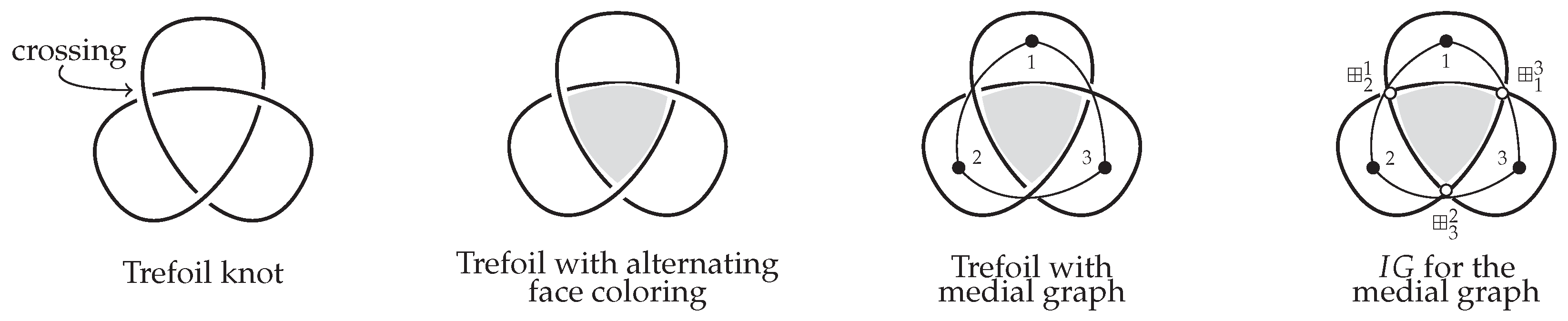
Mathematical knots are an embedding of a circle in . As with other topics in this note, the content here is very brief with more material regarding knots in [1] and [19]. A crossing in a knot is where one portion of the knot boundary, or strand, goes under another portion of the strand. Sometimes referred to as the unknot or the trivial knot, a circle is a knot that has no crossings. The knots that are the focus here are those that cannot be transformed into the unknot without cutting the knot’s strand. Figure 8 displays the trefoil knot on the left. Examine the displayed trefoil knot. Can this knot be transformed into a circle without cutting the strand?
Several graphs have been associated with knots, one of which is the medial graph. Note that the medial graph of a knot can be defined in different ways, one of which is given here. Assume that we have the trefoil knot as shown in Figure 8 projected onto . To form the medial graph of the trefoil graph, alternate two colors between adjacent faces of the knot as shown on the left center of Figure 8. In each of the white faces, place a vertex of the medial graph and connect the vertices that share a crossing with an edge as shown on the right center of the figure.
Now expand the trefoil back to with the medial graph in place. Consider the image in Figure 5 that shows in 3-D space with its three VIS. Ponder each VIS containing tangent incidence vectors. As the incidence definition of the medial graph establishes that edges exist based on shared crossings, place a at the crossing where i and j indicate the vertices that share the specific crossing. With the addition of the graphic connections, the medial graph becomes its . Can consideration of the tangent structure of the medial graph impact knot analysis? Can the vertex degree polynomial presented in the previous subsection apply to this situation? The answers to these questions are left to this note’s readers.
5. Conclusions
In this note, both simple connected G and G’s are defined on . Displayed by the incidence graph of a finite simple connected G, the incidence space can be considered the tangent bundle of G that is also a graph. If the vertices are defined as standard basis vectors, then all v are orthogonal to each other. Defined by open edge maps, each vertex v has a set of incidence vectors that are tangent to each other and tangent to v, while these vectors are orthogonal to all incidence vectors not incident to v, and orthogonal to all vertices other than v. The vectors at each specific v form a vector space as shown by the edge spaces of induced subgraphs formed from v and its incidence relations in . The vector space, formed by the tangent incidence vectors at each specific v, is the vertex incidence space (VIS) of v, and the graphic connection operator, connects the VIS in G to form the closed edges in G.
With much material left for further development by the readers of this note, an example that discusses effective communication and the information flow in a collaboration network is given. Ideas related to graph dimension are then covered, followed by polynomials assigned to edges that can be further explored by this note’s readers. A possible application to knot theory is also presented.
With full exploration of the following applications left to readers, consider spinor states and their relationship to graphs as outlined in [16]. Or assign the three dimensions of spacetime to the vertices of a simple connected graph, and let the graph edges reflect instantaneous time relationships (so undirected) between the vertices. What does the incidence graph say about the tangent space of the time structure? For non-instantaneous situations, what is the tangent structure of a directed graph? All possible applications for the tangent structure of a graph must be left to the future.
References
- Adams C.C.: The Knot Book: An Elementary Introduction to the Mathematical Theory of Knots. American Mathematical Society. (2004). [CrossRef]
- Ahmed H., Alwardi A., Salestina R.M.: On the vertex degree polynomial of graphs. TWMS Journal of Applied and Engineering Mathematics 13(1):232-245. (2023).
- Beineke L.W., Wilson R.J.: Topics in Algebraic Graph Theory. Cambridge University Press. Encyclopedia of Mathematics and its Applications #102 (2005).
- Biggs N.: Algebraic Graph Theory, 2nd Ed.. Cambridge University Press, Cambridge. (1993).
- Bishop R.L., Goldberg S.I.: Tensor Analysis on Manifolds. Dover Publications, Garden City, New York. (1968).
- Carroll S.: Spacetime and Geometry: An Introduction to Genral Relativity. Cambridge University Press, Cambridge. (2019).
- Chartrand G., Lesniak L., Zhang P.: Graphs & Digraphs, 6th Ed.. CRC Press, Boca Raton, FL. (2016).
- Cvetkovicć D., Rowlinson P., Simić S.: An Introduction to the Theory of Graph Spectra. Cambridge University Press, Cambridge. (2010).
- Diestel R.: Graph Theory, 6th Ed.. Springer, Berlin. (2025).
- Erdös P., Harary F., Tutte W.T.: On the dimension of a graph. Mathematika.12, 118-122. doi:10.1112/S0025579300005222 (1965). [CrossRef]
- Feynman R.: Space-time approach to non-relativistic quantum mechanics. Review of Modern Physics. 20(2) 367-387. doi:10.1103/RevModPhys.20.367 (1948). [CrossRef]
- Fleisch D.: A Student’s Guide to vectors and Tensors. Cambridge University Press, Cambridge. (2012).
- Godsil C., Royle G.: Algebraic Graph Theory. Springer-Verlag, New York. (2001).
- Gould R.: Graphs and vector spaces. Journal of Mathematics and Physics. v37: 193-214. (1958). [CrossRef]
- Gross G., Meinrenken E.: Manifolds, Vector Fields, and Differentiable Forms. Springer Undergraduate Mathematics Series. Springer Nature, Switzerland. (2023).
- Harris G.M., Staples G.S..: Spinorial Formulations of Grap[h Problems. Advances in Applied Clifford Algebras. Springer Nature. 22: 59–77. https://doi.org/10.1007/s00006-011-0298-0 (2012). [CrossRef]
- Holly M.: Collaboration: people, papers, average graphs, Durfee squares and metric dimension. Social network analysis and mining. Springer Nature. 16(59) doi:10.1007/s13278-026-01595-3 (2026). [CrossRef]
- Levi F.W.: Finite geometrical systems. Calcutta University Press, Calcutta. (1942).
- Murasugi K.: Knot Theory & Its Applications. Modern Birkhäuser Classics. Birkhäuser, Boston. (2000).
- Newman M.E.J.:The structure of scientific collaboration networks. PNAS. 98(2): 404-409. doi:10.1073/pnas.98.2.404 (2001). [CrossRef]
- Pinsanski T., Servatius B.: Configurations from a Graphical Viewpoint. Birkhäuser, Springer, New York. (2013).
- Polster B.: A Geometrical Picture Book. Springer-Verlag New York. (1991).
- Robbin J.W., Salamon D.A.: Introduction to Differential Geometry. Springer Studium Mathematik (Master) Series. Springer-Verlag, Berlin. (2022).
- Wallis W.D: A Beginner’s Guide to Graph Theory, 2nd Ed. Birkhäuser, Boston. (2007).
Figure 1.
Index placement description for open edges in graph G.
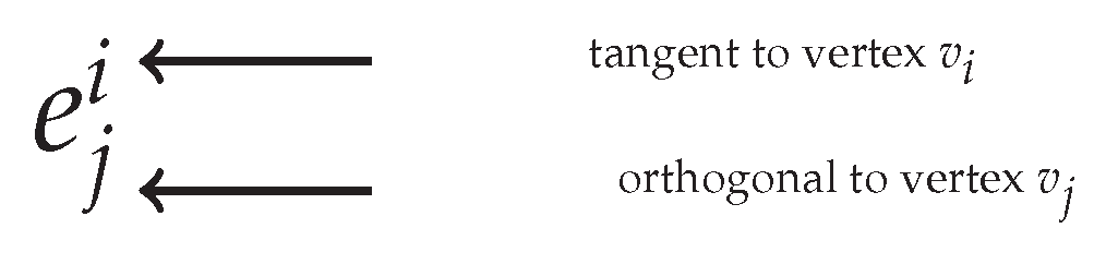
Figure 2.
An example graph G with G’s incidence matrix, , adjacency matrix, and G’s CNM based on nonadjacent vertices.
Figure 2.
An example graph G with G’s incidence matrix, , adjacency matrix, and G’s CNM based on nonadjacent vertices.
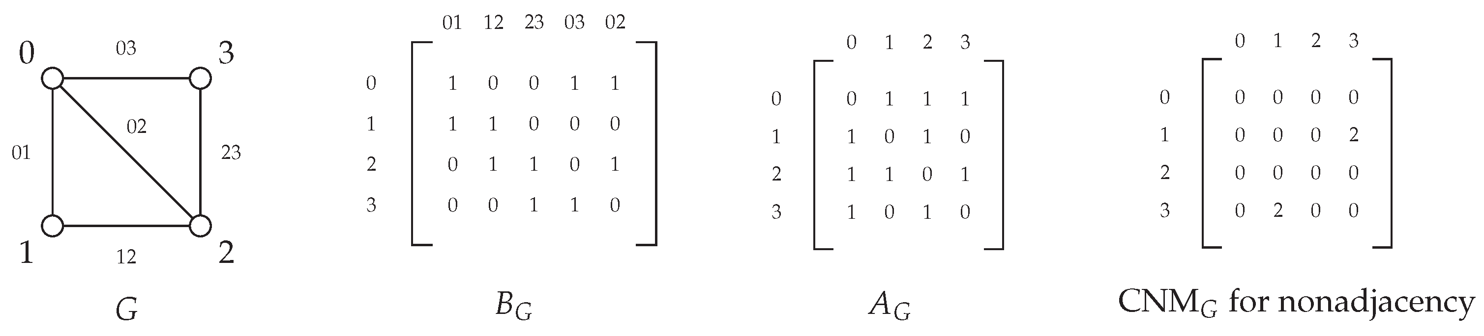
Figure 3.
An example graph G with its related , plus ’s CNM and .
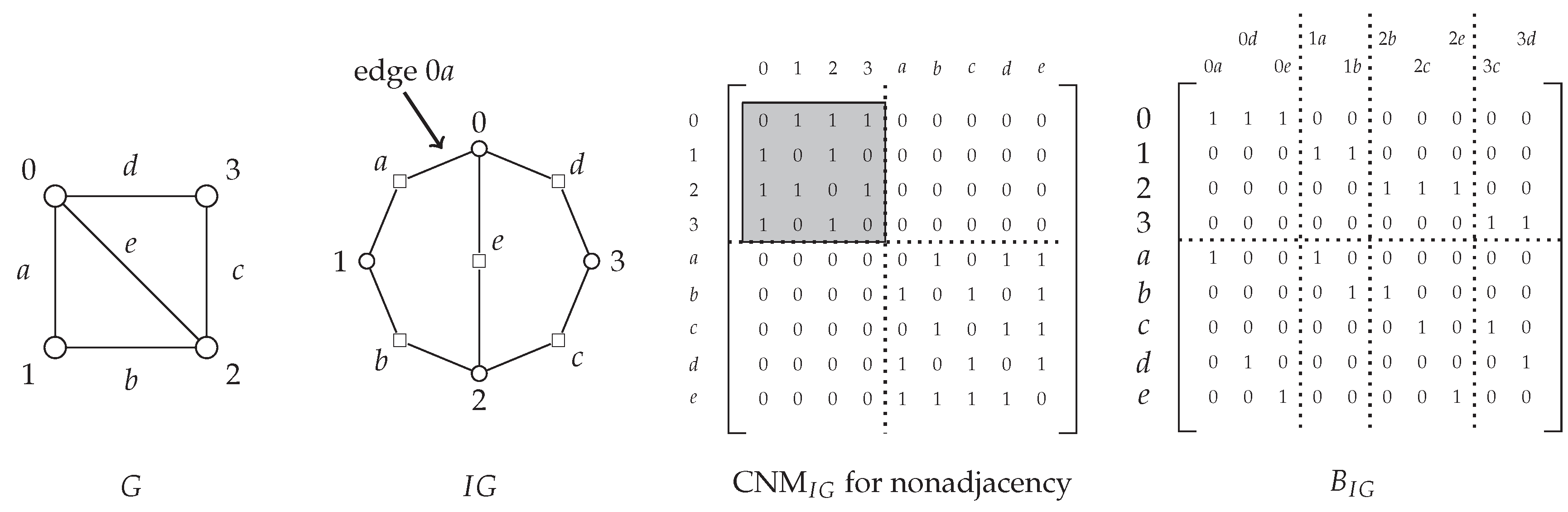
Figure 4.
Graph G, G’s incidence graph and the tangent spaces found in that form G’s graph.
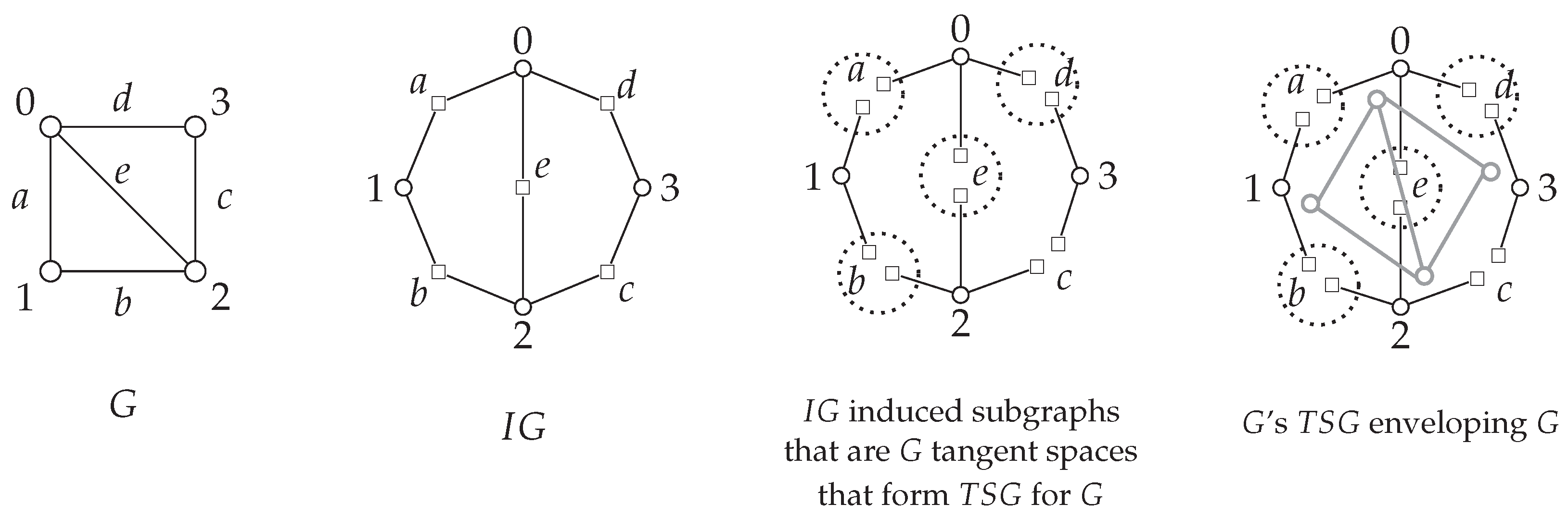
Figure 5.
For graph on the left center, the VIS are in the right center and the for on the right reflects the connections in .
Figure 5.
For graph on the left center, the VIS are in the right center and the for on the right reflects the connections in .
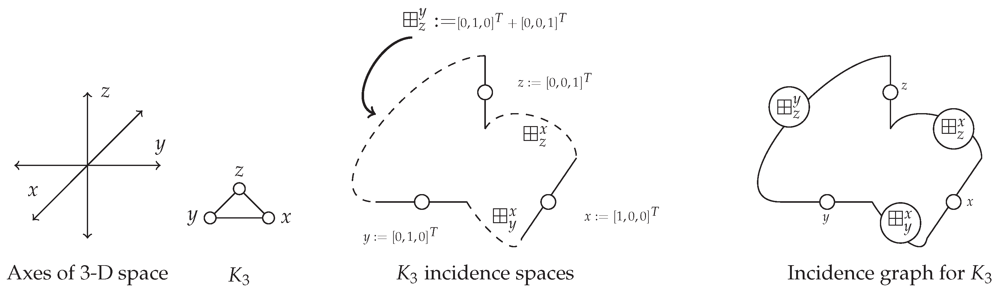
Figure 6.
Impact on the incidence vector space of vertex X by creation from bipartite containing authors and distinct research groups.
Figure 6.
Impact on the incidence vector space of vertex X by creation from bipartite containing authors and distinct research groups.
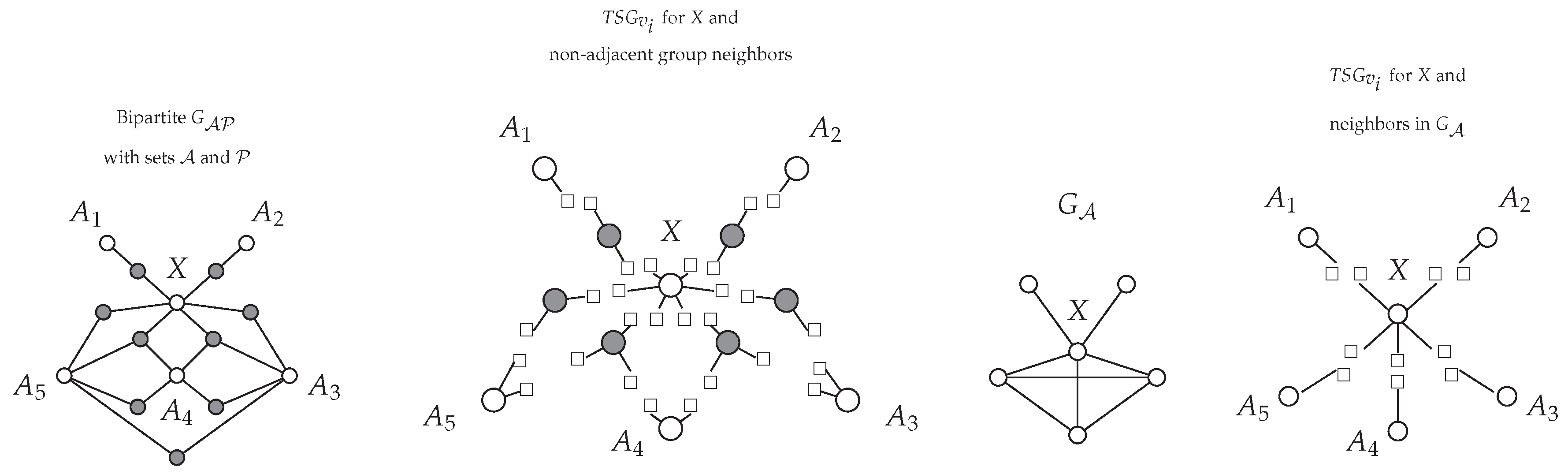
Figure 7.
Polynomials applied to the each in G’s .
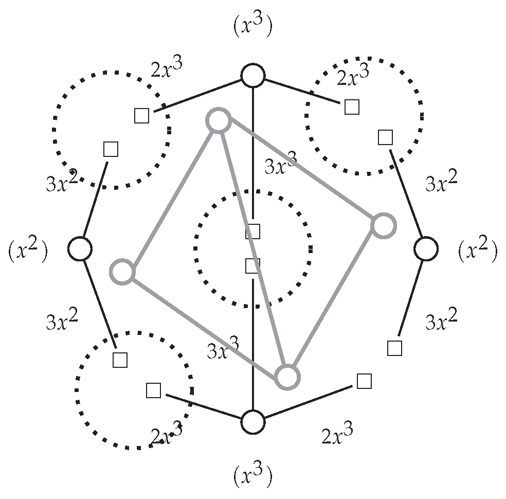
Figure 8.
Trefoil knot with a alternating coloring of adjacent faces and the knot’s medial graph.
Disclaimer/Publisher’s Note: The statements, opinions and data contained in all publications are solely those of the individual author(s) and contributor(s) and not of MDPI and/or the editor(s). MDPI and/or the editor(s) disclaim responsibility for any injury to people or property resulting from any ideas, methods, instructions or products referred to in the content. |
© 2026 by the authors. Licensee MDPI, Basel, Switzerland. This article is an open access article distributed under the terms and conditions of the Creative Commons Attribution (CC BY) license (http://creativecommons.org/licenses/by/4.0/).
Copyright: This open access article is published under a Creative Commons CC BY 4.0 license, which permit the free download, distribution, and reuse, provided that the author and preprint are cited in any reuse.