
Submitted:
27 September 2026
Posted:
01 October 2026
You are already at the latest version
Abstract
There are now tens of thousands of tracked objects in orbit, and someone has to check them all for near-misses. The simple way compares every object with every other one, which scales as O(N²). For the 15,830 active objects we look at here, that's over 125 million checks per snapshot—far too many to repeat around the clock. This paper builds and benchmarks a Python pipeline that does the job faster using two ideas from high performance computing: spatial partitioning and parallel processing. We pulled real two-line element data from CelesTrak and propagated it with SGP4. On the full catalog, grid and k-d tree methods checked about 61× fewer pairs than brute force—and found the same 211 close pairs, with zero disagreement. A 24-hour time-window screen picked up real conjunctions and, as a sanity check, correctly flagged co-located structures like the ISS modules and the TanDEM-X/TerraSAR-X formation. Parallelizing the real workload gave a 3.7× speedup on four cores at over 92% efficiency; past that, overhead took over, just as Amdahl's law predicts. Detections stayed identical across every core count, so the parallel version is provably correct. We also estimate each pair's probability of collision, and the headline is simple: the riskiest pair isn't the closest one. Finally we added time-of-closest-approach refinement, a red/yellow/green triage, single-asset screening, and a screen against real debris from the Fengyun-1C, Iridium-33, and Cosmos-1408 break-ups—which turned up a working Starlink satellite passing within 4.4 km of 2009 collision debris.
Keywords:
conjunction assessment
; space debris
; high performance computing
; spatial partitioning
; parallel computing
; SGP4
; collision probability
; strong scaling
; weak scaling
; Amdahl’s law
I. Introduction
Low Earth orbit is getting crowded. Big commercial constellations, plus decades of debris from spent rockets and old collisions, have pushed the number of tracked objects into the tens of thousands. And every one of them needs watching. Space-surveillance teams run conjunction assessment around the clock: for each object, will anything pass dangerously close in the next stretch of time? If so, operators get a warning and can plan a dodge. The orbital mechanics behind all of this is standard textbook material [1].
The hard part is that, done directly, this is an all-pairs problem. To be sure you miss nothing, you compare every object with every other—N(N−1)/2 checks, which grows with the square of N. For our 15,830 objects that’s over 125 million checks for a single snapshot. Repeat that across many time steps, forever, and brute force falls apart.
So we ask a simple question: how do you make it fast? We lean on two HPC ideas. The first is algorithmic. Spatial partitioning splits space into cells, so each object only gets compared with nearby ones—dropping the cost toward O(N·k) for a small neighbor count k. The second is architectural: spread the work across CPU cores. Our contributions are a reproducible Python pipeline on real data, a head-to-head comparison of naive, k-d tree, and grid screening checked for correctness on the full catalog, a 24-hour time-window screen, and strong- and weak-scaling studies that show both the speedup and where it stops paying off.
II. Background
A. Orbital Propagation and SGP4
Orbital objects are usually published as two-line element sets, or TLEs—a compact snapshot of the orbit at some reference time. To get an actual position you run the TLE through a propagation model. SGP4 is the standard one [2,4], and it handles the main perturbations on near-Earth orbits. We use it to turn each TLE into an Earth-centered inertial (ECI) position.
B. All-Pairs Proximity and Spatial Data Structures
Finding close pairs is a well-worn problem. Brute force checks every distance—exact, but quadratic. Smarter structures use the obvious fact that only nearby things can be close. A grid drops each object into a cell and only checks its own cell and the 26 around it. A k-d tree splits space along alternating axes for fast neighbor queries [5]. Both win big when objects are spread unevenly, and orbits are very uneven.
C. Parallelism and Amdahl’s Law
Parallel computing cuts wall-clock time by splitting work across cores. But there’s a ceiling. Amdahl’s law [8] says that if a fraction p of the work can run in parallel, the best speedup on c cores is 1 / ((1−p) + p/c). Some part is always serial, and overheads like starting processes and moving data add up. So the speedup curve bends away from ideal as you add cores. Measuring where it bends is the whole point of a scaling study.
III. Methodology
A. Data
We pulled real orbital data from CelesTrak [3], which publishes current TLE catalogs. Parsing the active-object list gave 15,830 valid objects. For each we recorded inclination, mean motion, and a rough altitude. Figure 1 shows the spread—a thick band in low Earth orbit and a second clump out at geostationary.
B. Propagation
Each TLE was propagated to a common epoch with python-sgp4 [4], giving an ECI position in kilometers. For the controlled method comparison we used a 2,000-object subset—big enough to show the trend, small enough to keep brute force tractable. The scale and correctness tests use the full catalog. Figure 2 shows two clear populations: a dense low shell and a sharp geostationary ring near 42,000 km.
C. Screening Algorithms
We built three. The naive baseline computes every pairwise distance with vectorized NumPy [7]. The grid method hashes objects into cubic cells sized a few times the threshold, checking each one only against its own cell and the 26 neighbors. The third uses SciPy’s k-d tree [6], whose query-pairs call returns everything within the threshold.
D. Time-Window Screening
To match how operators actually work, the time-window screen walks every object across 24 hours in fixed steps. For each flagged pair it records the closest separation and when it happens. We used a 25 km threshold. Pairs that get within 0.5 km are treated as self-conjunctions—bits of one physical structure sitting together—and reported separately from real distinct-object approaches.
E. Parallelization and Setup
The time-window screen is naturally parallel: each time step is its own task. We hand tasks to a pool of worker processes, ship the propagation objects to each worker once at startup, and batch tasks into chunks so the work per dispatch stays large next to the communication cost. Everything ran on a laptop with a 16-logical-core CPU on Ubuntu. Times are wall-clock, averaged over three runs. Speedup is against single-core time, and efficiency is speedup over core count.
IV. Results and Discussion
A. Quadratic Cost of the Baseline
The naive method behaves exactly as you’d expect. Figure 3 shows execution time climbing faster than linearly with object count, the pair count ballooning like a parabola, and time tracking the pair count almost perfectly straight. That last line is the giveaway of an O(N²) algorithm—the cost is the pair count, nothing else.
B. Full-Catalog Screening and Correctness
Run the spatial methods on all 15,830 objects and two things show up: it’s feasible, and it’s correct. Brute force would need 125,286,535 comparisons—not something you repeat continuously. The spatial methods check around two million candidate pairs instead, roughly 61× fewer. And here’s the important bit: grid and k-d tree returned identical results, 211 close pairs each, with zero found by only one method. No false negatives. Figure 4 sums it up.
That single snapshot found just 211 pairs—far fewer than the time-window screen below. A frozen moment misses pairs that get close at other times. That’s exactly why you screen over a window.
C. Time-Window Conjunction Detection
Over 24 hours the screen flagged 26 close-approach pairs. Eleven were self-conjunctions; 15 were genuinely distinct objects, and 3 of those came inside 10 km. The self-conjunction filter doubles as a validation. It correctly pulled out the co-located ISS modules—ZARYA, UNITY, ZVEZDA, DESTINY—and POISK, plus the TanDEM-X/TerraSAR-X pair, which fly in tight formation on purpose. Catching known co-located hardware is good evidence the screen behaves physically.
The real approaches make physical sense too. The closest, 3.59 km, is between two O3b satellites sharing an orbital plane. Next, 8.43 km, between two Magnetospheric Multiscale satellites that fly in formation. Then 9.92 km between two co-located GEO comms satellites. So the tightest approaches are mostly intentional proximity—constellations, formations, shared GEO slots—which is exactly the pattern real systems have to sort through. Table 1 lists them; Figure 5 visualizes them.
D. Risk-Based Prioritization
Finding close pairs is only half the job. Operators don’t act on distance alone—a small miss isn’t always dangerous, and a bigger one isn’t always safe. What matters is the probability of collision, Pc, which blends the miss distance with how uncertain each position is. We compute Pc for every genuine pair using the standard 2D short-encounter (Foster) method [10,11]. TLEs carry no uncertainty, so we assign representative values by orbit regime—and we’ll say it plainly: these are modeled, not measured.
The result is the most striking thing we found. The riskiest pair isn’t the closest. Our highest Pc, about 5.6×10⁻⁵, came from a pair 16.5 km apart—while a pair just 3.6 km apart scored lower. Pc depends on the encounter geometry and the uncertainty, not distance by itself. Rank by distance alone and you’d push the wrong events to the top. Figure 6 shows it: the highest-Pc points don’t sit at the smallest distances.
And it’s worth saying what we didn’t find. Nothing crossed the usual 10⁻⁴ action threshold over the window. That’s the reassuring answer. Real maneuver-worthy conjunctions are rare, and most of our close approaches are satellites flying near each other on purpose. A screen lighting up with imminent collisions across the active catalog would more likely mean a bug than an emergency.
E. Parallel Strong Scaling
We benchmarked the parallel screen on the real workload: 1,500 objects across 289 time steps, 433,500 SGP4 evaluations. Table 2 has the numbers. Up to four cores the speedup tracks the ideal line closely, holding above 92% efficiency. Then it bends. Efficiency drops to about 55% at eight cores and 33% at sixteen, while the absolute time barely moves. One detail matters a lot: the detection count, 6,167, was identical at every core count. Parallelism changed the speed, not the answer.
Figure 7.
Strong scaling on the real workload: speedup versus cores (left) and parallel efficiency (right). Source: github.com/Aditya29072002/Satellite-Conjunction-Assessment — outputs/polished_scaling.png.
Figure 7.
Strong scaling on the real workload: speedup versus cores (left) and parallel efficiency (right). Source: github.com/Aditya29072002/Satellite-Conjunction-Assessment — outputs/polished_scaling.png.
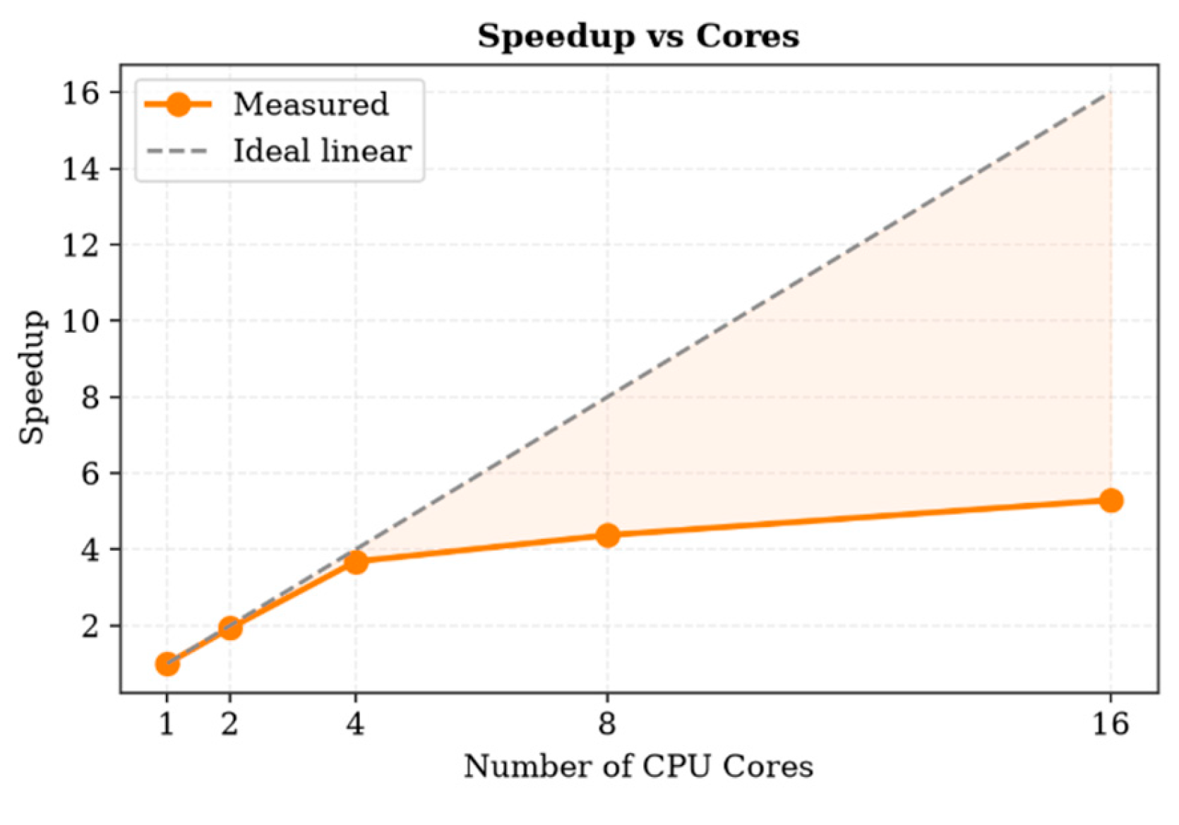
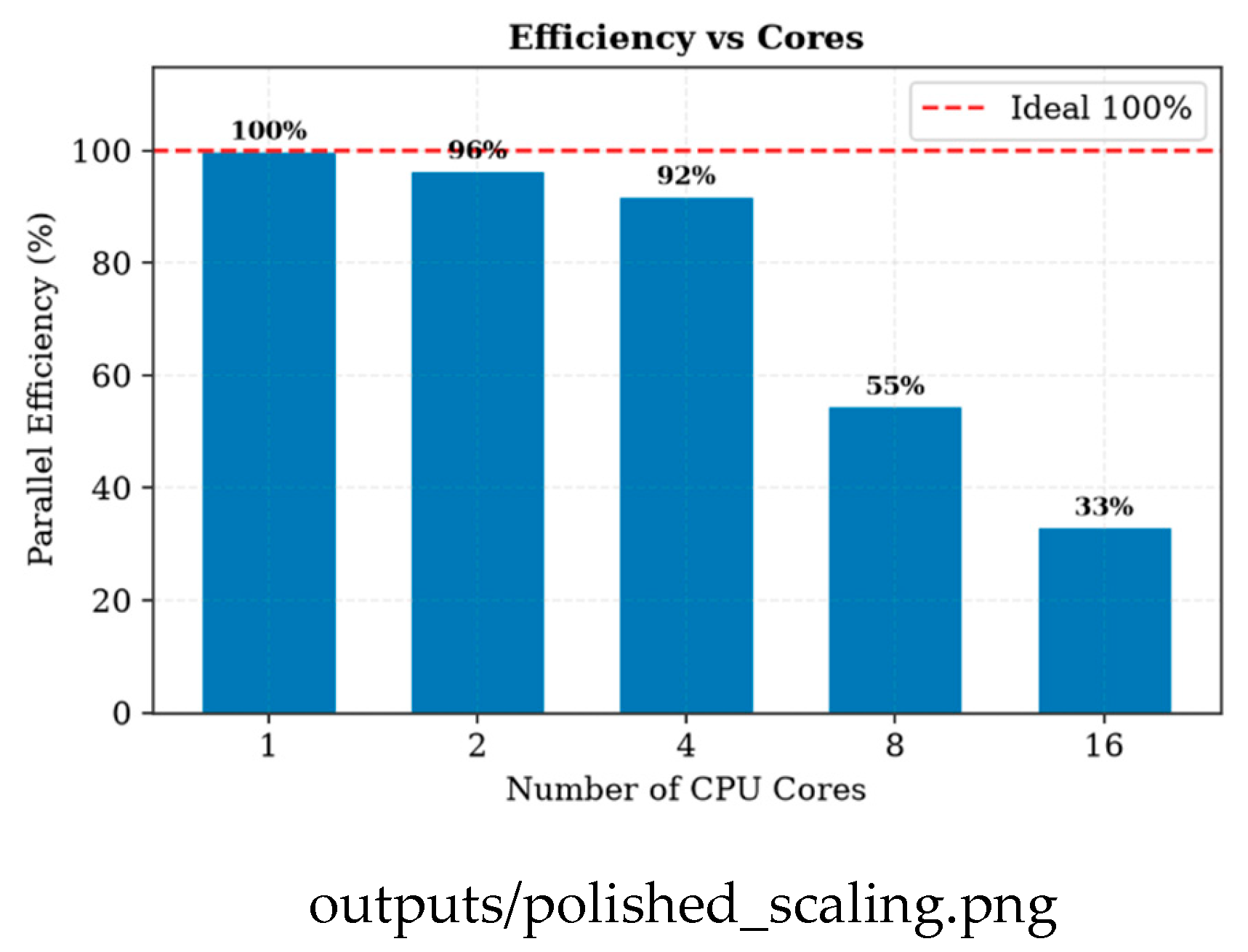
This is Amdahl’s law in action. Add workers and the fixed costs—starting processes, shipping data, gathering results—eat a bigger slice of a shrinking runtime, so the serial part takes over sooner. The practical takeaway is a sweet spot around four to eight cores. Past that, more cores buy you almost nothing.
F. Weak Scaling
Weak scaling fixes the work per core—30 time steps each—and grows the problem with the core count, so flat time is ideal. Table 3 shows time holding nearly flat through four cores (0.419 s to 0.430 s, above 97%), then rising to 38.8% efficiency at sixteen. The same four-core knee turns up in strong scaling, weak scaling, and the real workload. Three different experiments, one consistent answer—which makes the recommended range solid rather than a fluke.
Figure 8.
Weak scaling: execution time and efficiency as the problem grows with the core count. Source: github.com/Aditya29072002/Satellite-Conjunction-Assessment — outputs/phase7_weakscaling.png.
Figure 8.
Weak scaling: execution time and efficiency as the problem grows with the core count. Source: github.com/Aditya29072002/Satellite-Conjunction-Assessment — outputs/phase7_weakscaling.png.
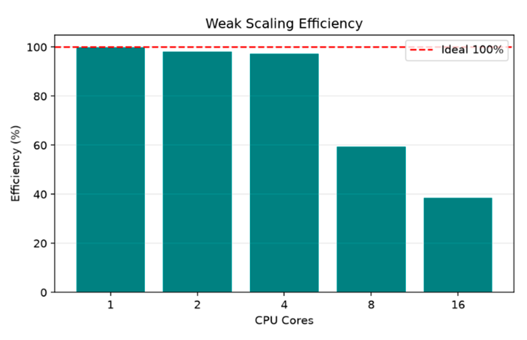
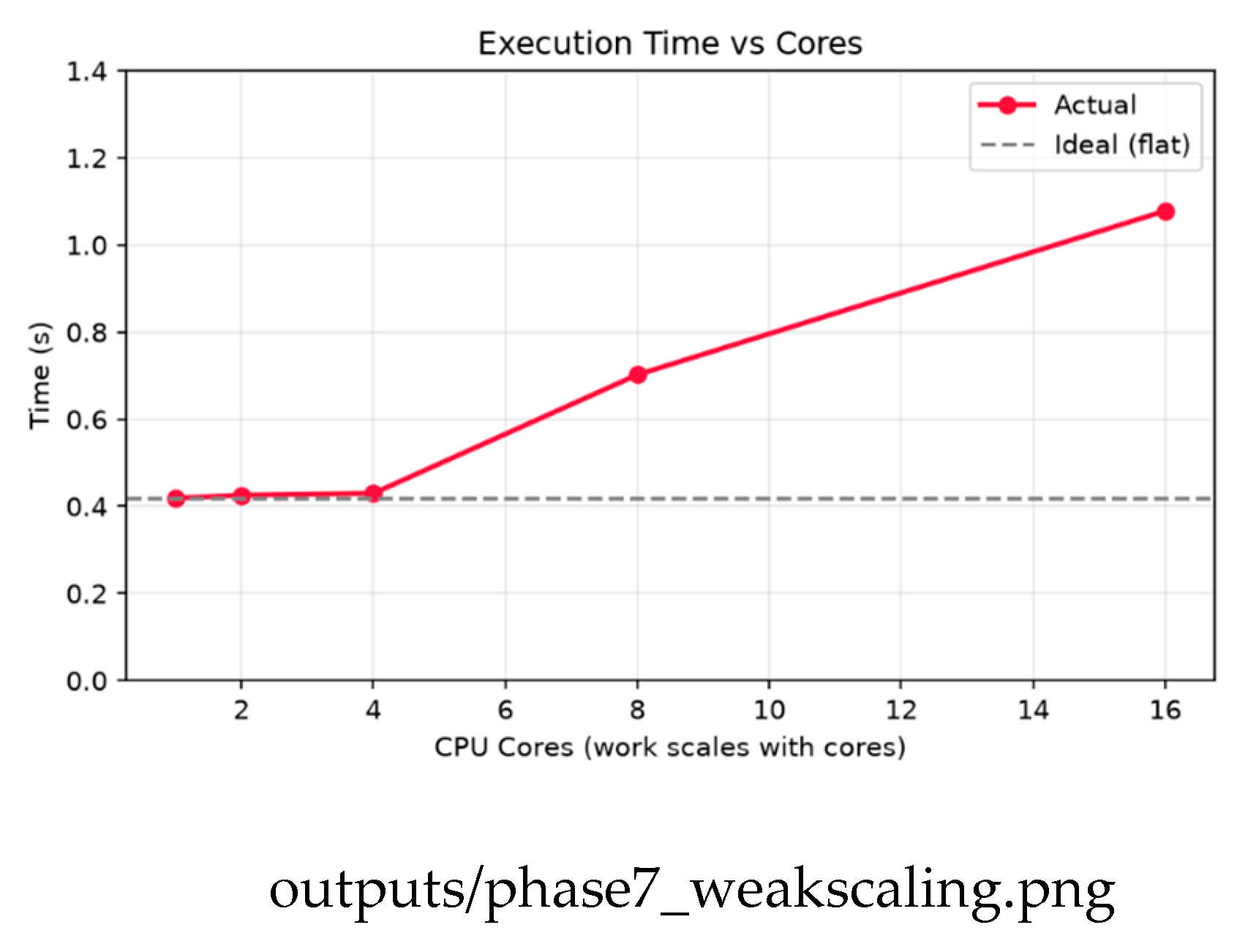
G. Operational Extensions
To make this feel less like a benchmark and more like a working tool, we added four features.
First, sharper timing. The screen samples distance at fixed steps, so the true closest moment usually falls between two samples. Fit a parabola through the closest sample and its neighbors and you get a better estimate—a sub-step time and a slightly smaller miss. The ANIK F3 / ECHOSTAR 15 approach tightened from 5.17 km to 4.88 km this way. It only adjusts when the closest point has neighbors on both sides; sharp single-step approaches keep their sampled value. That’s the honest behavior.
Second, a simple triage. Each pair gets a red, yellow, or green label from its Pc and miss distance—red over the action threshold, yellow in a watch band, green otherwise. Over the window we got no red, four yellow, the rest green. That’s the expected picture for an active catalog. The triage feeds a plain-text report listing each event with its objects, time of closest approach, probability, and color—the kind of thing a real operator would actually receive.
Third, flip the question. Instead of “which pairs are close?” ask “what threatens my satellite?” Real services screen one protected asset against the whole catalog. We screened the ISS that way and got a clean result: one object came near it over the window, at a comfortable distance. Just what you’d hope for something watched that closely. Figure 9 shows the same idea as approach curves—separation rising and falling across the window, dipping to a clear minimum at closest approach.
Fourth, and the big one: real debris. We pulled fragment catalogs for three historic break-ups from CelesTrak [3]—the Fengyun-1C anti-satellite test (2007), the accidental Iridium-33 collision (2009), and the Cosmos-1408 anti-satellite test (2021). Mixed with active satellites, the screen found tens of active-versus-debris close approaches. The closest was a working Starlink satellite passing within about 4.4 km of an Iridium-33 fragment, with Earth-observation satellites like Sentinel-3A and MetOp-B near Fengyun-1C debris. This is the part that matters most, because debris can’t move, and the long-term growth of these fragment populations is a recognized hazard [9]. When an active satellite nears a fragment, only the satellite can act. Figure 10 shows the active-versus-debris field.
V. Limitations
A few honest caveats. The collision probabilities rest on two simplifications. First, the position uncertainties are modeled by orbit regime, not measured—TLEs don’t carry that data—so the Pc values show off the method rather than giving operational risk. Second, the 2D Foster method assumes a fast, near-straight encounter. That’s fine for quick LEO crossings but weaker for slow GEO co-locations.
There’s more. The screen takes the minimum across sampled time steps rather than interpolating the true closest approach from relative velocity, so the closest-approach times are only as precise as the sampling—though the parabolic refinement helps. The debris run uses a representative subset of fragments and active objects, so its counts illustrate the threat rather than counting every piece. The method comparison uses a 2,000-object subset, while the scale and correctness results use the full catalog. And the parallel code leans on Python multiprocessing, whose per-process overhead is heavy; a compiled or shared-memory version would likely push the sweet spot to more cores. None of these break the findings—they just point to where to go next.
VI. Conclusion
We built a reproducible Python pipeline for satellite conjunction assessment on real CelesTrak data and SGP4. On the full 15,830-object catalog, the spatial methods checked about 61× fewer pairs than brute force and returned identical close-pair sets—fast and correct at scale. A 24-hour screen recovered real conjunctions and, as a check, nailed co-located structures like the ISS modules and the TanDEM-X/TerraSAR-X formation. Adding collision probability moved the tool from “how close?” to “how risky?”—and showed the most dangerous pair wasn’t the closest, which a distance-only screen would miss. Parallelizing the real workload hit near-ideal speedup to four cores, then bent away beyond eight, right on cue with Amdahl’s law and backed up by both scaling studies. Detections stayed identical across all core counts, so the parallel version is correct. We pushed it further into something operational—sub-step timing, risk triage, single-asset screening, and a real-debris screen that turned up a current Starlink satellite within about 4.4 km of 2009 Iridium-33 debris. Put together, it shows how a couple of HPC ideas crack a real aerospace problem—and why it’s worth reporting not just your peak speedup but the point where extra cores stop helping.
References
- D. Vallado, Fundamentals of Astrodynamics and Applications, 4th ed. Hawthorne, CA: Microcosm Press, 2013.
- F. R. Hoots and R. L. Roehrich, “Models for propagation of NORAD element sets,” Spacetrack Report No. 3, U.S. Air Force, 1980.
- T. S. Kelso, “CelesTrak: Current NORAD two-line element sets.” [Online]. Available: https://celestrak.org.
- B. Rhodes, “sgp4: Track Earth satellites from TLE data using the SGP4 model,” Python package. [Online]. Available: https://pypi.org/project/sgp4.
- Bentley, J. L. Multidimensional binary search trees used for associative searching. Commun. ACM 1975, vol. 18(no. 9), 509–517. [Google Scholar] [CrossRef]
- Virtanen, P.; et al. SciPy 1.0: fundamental algorithms for scientific computing in Python. Nat. Methods 2020, vol. 17, 261–272. [Google Scholar] [CrossRef]
- Harris, C. R.; et al. Array programming with NumPy. Nature 2020, vol. 585, 357–362. [Google Scholar] [CrossRef]
- G. M. Amdahl, “Validity of the single processor approach to achieving large scale computing capabilities,” in Proc. AFIPS Spring Joint Computer Conf., 1967, pp. 483–485.
- Liou, J.-C. An active debris removal parametric study for LEO environment remediation. Adv. Space Res. 2011, vol. 47(no. 11), 1865–1876. [Google Scholar] [CrossRef]
- Akella, M. R.; Alfriend, K. T. Probability of collision between space objects. J. Guid. Control Dyn. 2000, vol. 23(no. 5), 769–772. [Google Scholar] [CrossRef]
- F. K. Chan, Spacecraft Collision Probability. El Segundo, CA: The Aerospace Press, 2008.
Figure 1.
The acquired catalog (15,830 objects): orbital inclination, derived altitude, and mean motion versus altitude. Source: github.com/Aditya29072002/Satellite-Conjunction-Assessment — outputs/phase1_dataset_overview.png.
Figure 1.
The acquired catalog (15,830 objects): orbital inclination, derived altitude, and mean motion versus altitude. Source: github.com/Aditya29072002/Satellite-Conjunction-Assessment — outputs/phase1_dataset_overview.png.
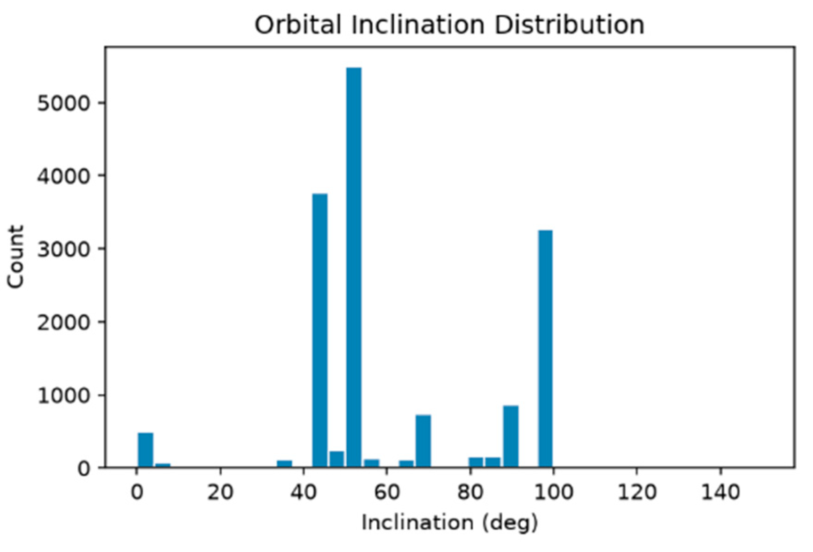
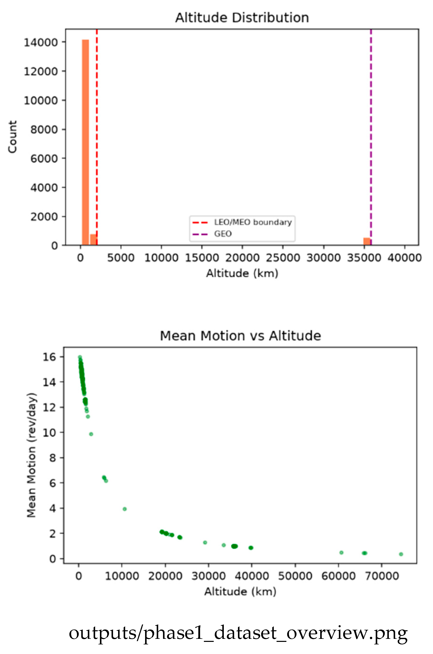
Figure 2.
Propagated positions: 3D distribution, equatorial projection, and altitude histogram. Source: github.com/Aditya29072002/Satellite-Conjunction-Assessment — outputs/phase2_positions.png.
Figure 2.
Propagated positions: 3D distribution, equatorial projection, and altitude histogram. Source: github.com/Aditya29072002/Satellite-Conjunction-Assessment — outputs/phase2_positions.png.
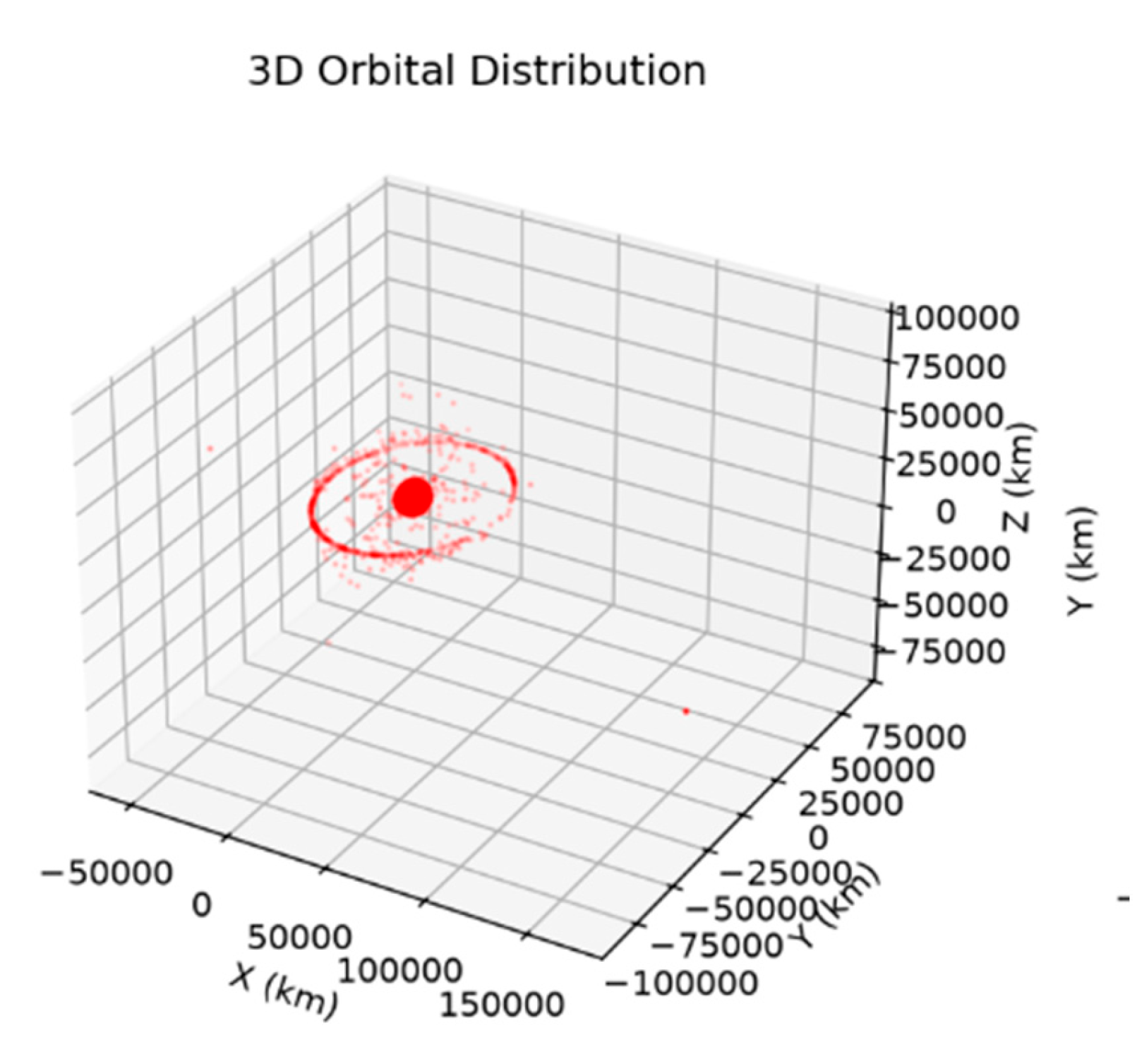
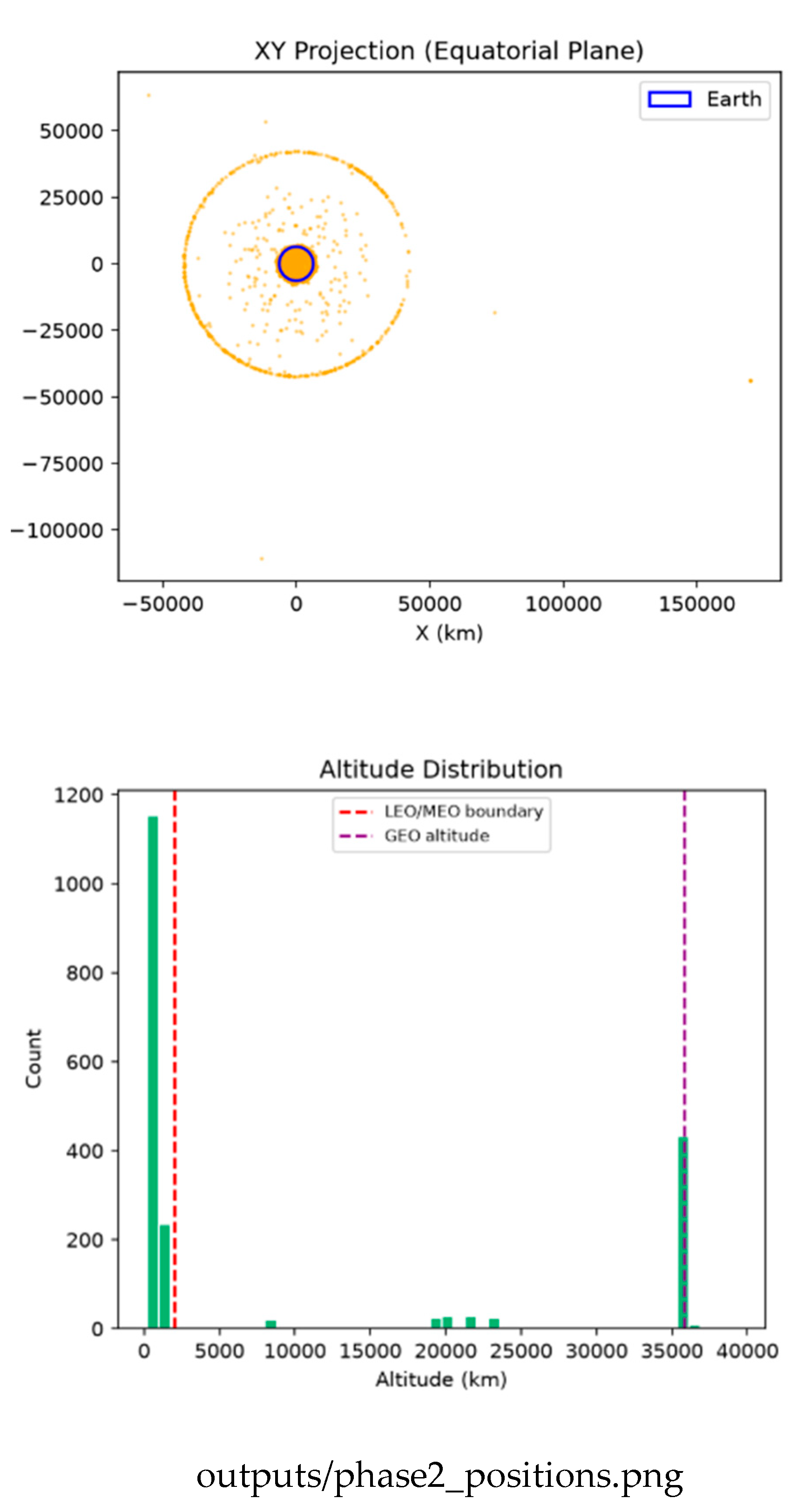
Figure 3.
Naive O(N²) baseline: time versus object count, pair-count growth, and the near-linear link between time and pairs examined. Source: github.com/Aditya29072002/Satellite-Conjunction-Assessment — outputs/phase3_naive_benchmark.png.
Figure 3.
Naive O(N²) baseline: time versus object count, pair-count growth, and the near-linear link between time and pairs examined. Source: github.com/Aditya29072002/Satellite-Conjunction-Assessment — outputs/phase3_naive_benchmark.png.
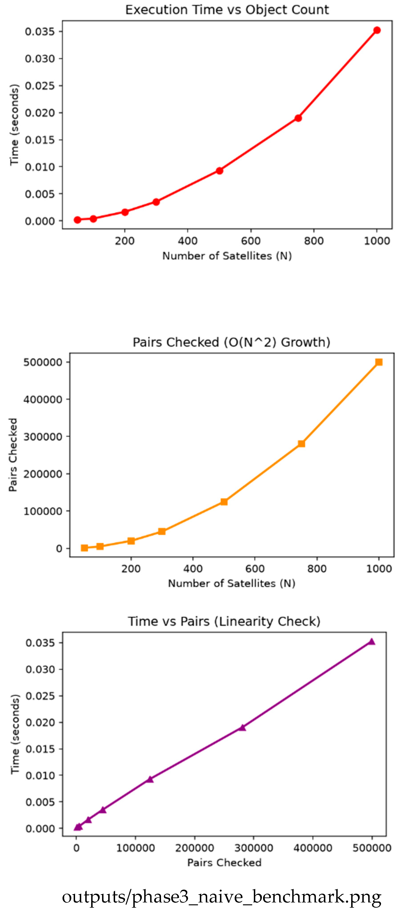
Figure 4.
Full-catalog screening (15,830 objects): equatorial distribution, comparison counts on a log scale, and close-approach distances. Grid and k-d tree agree exactly (211 pairs, zero disagreement). Source: github.com/Aditya29072002/Satellite-Conjunction-Assessment — outputs/phase9_fullcatalog.png.
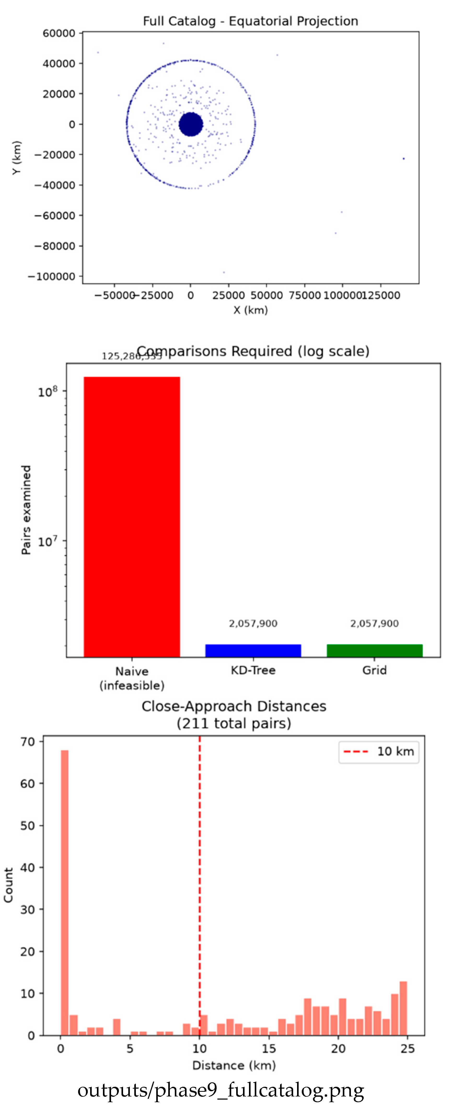
Figure 5.
Genuine distinct-object conjunctions over 24 hours: minimum approach distance, time of closest approach, and distance versus time. Source: github.com/Aditya29072002/Satellite-Conjunction-Assessment — outputs/phase6_filtered.png.
Figure 5.
Genuine distinct-object conjunctions over 24 hours: minimum approach distance, time of closest approach, and distance versus time. Source: github.com/Aditya29072002/Satellite-Conjunction-Assessment — outputs/phase6_filtered.png.
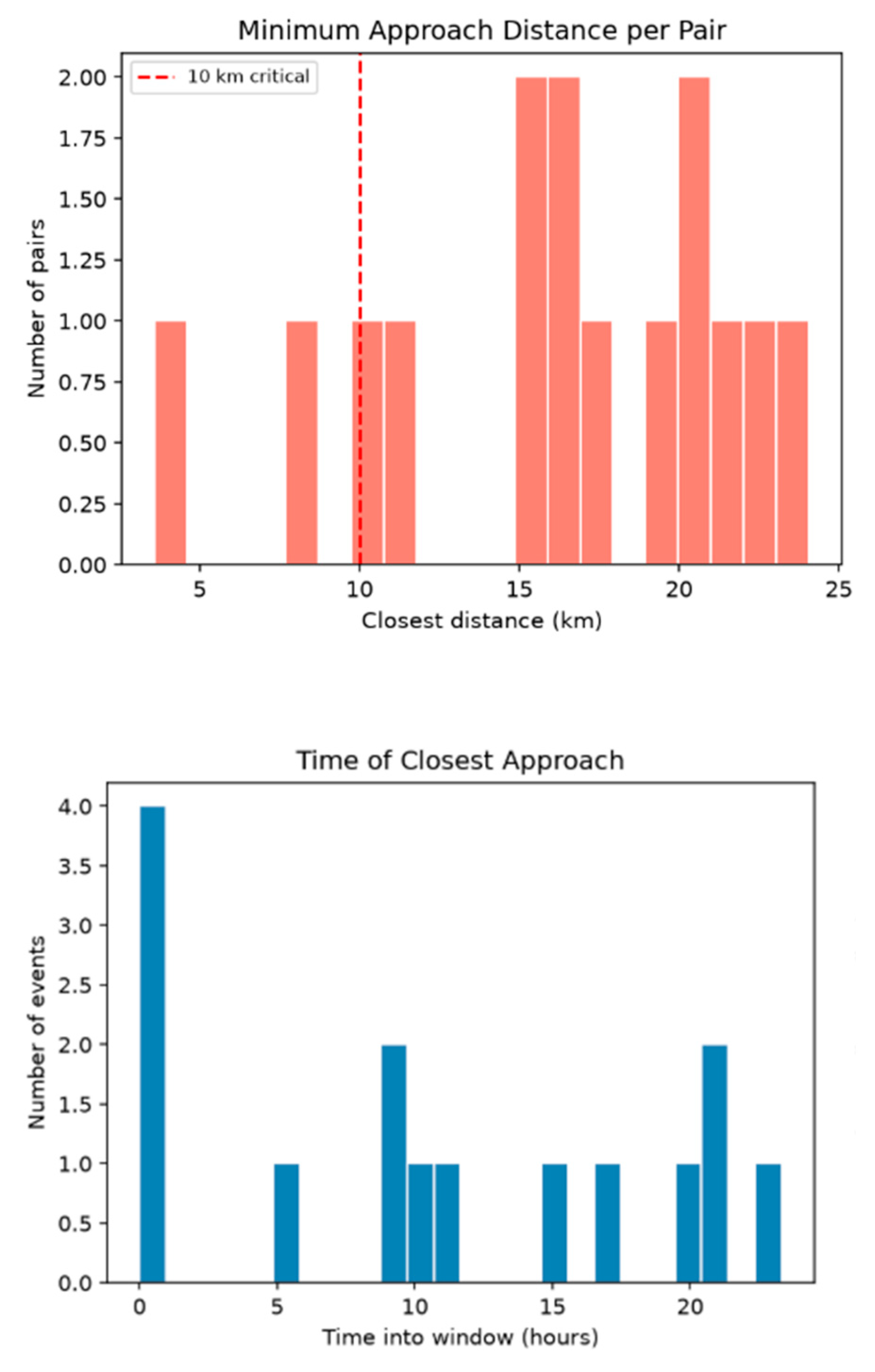
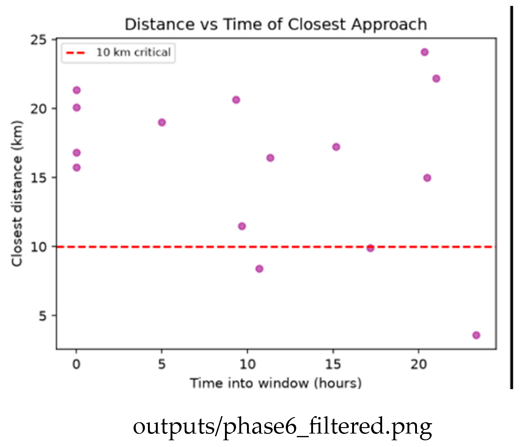
Figure 6.
Collision probability: Pc versus miss distance (left) and the distribution of probabilities (right). The highest-Pc points are not the closest ones. Source: github.com/Aditya29072002/Satellite-Conjunction-Assessment — outputs/phase11_collision_probability.png.
Figure 6.
Collision probability: Pc versus miss distance (left) and the distribution of probabilities (right). The highest-Pc points are not the closest ones. Source: github.com/Aditya29072002/Satellite-Conjunction-Assessment — outputs/phase11_collision_probability.png.
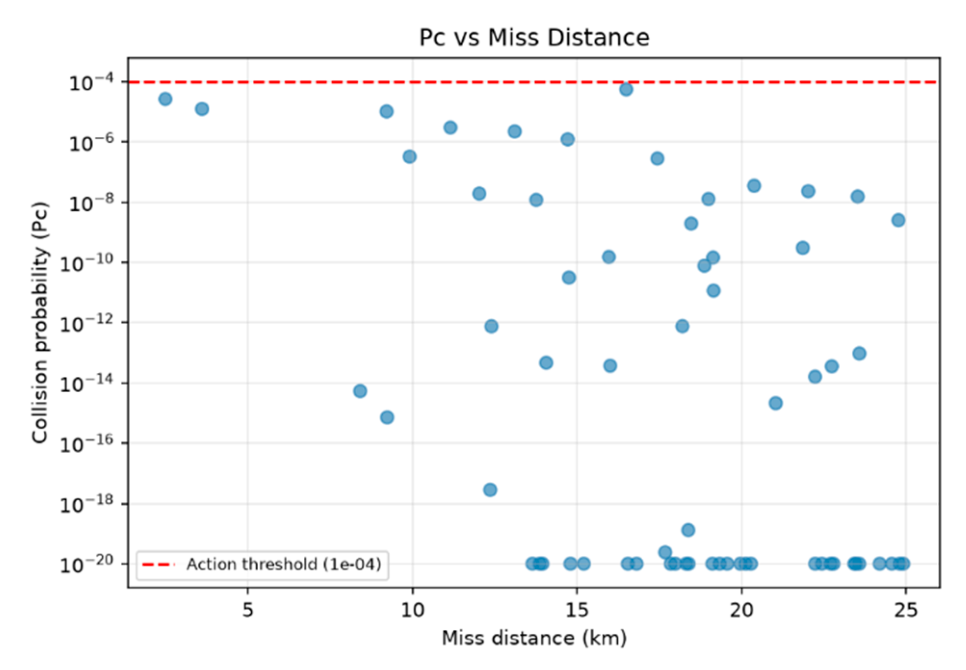
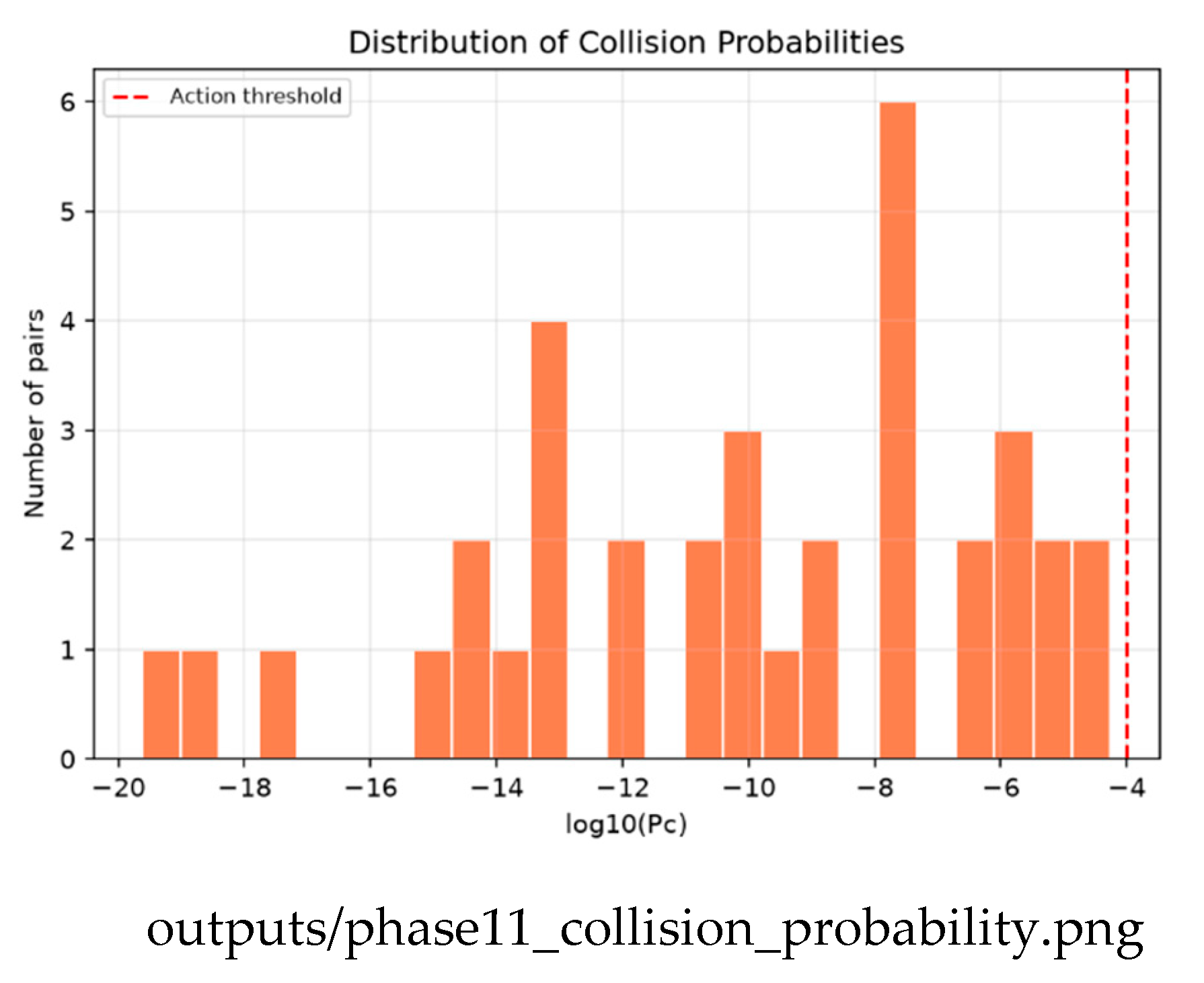
Figure 9.
Approach curves for selected pairs: separation over 24 hours, with the closest approach marked. GEO pairs show slow, smooth curves; MEO constellation members re-approach more sharply. Source: github.com/Aditya29072002/Satellite-Conjunction-Assessment — outputs/phase15_approach_curves.png.
Figure 9.
Approach curves for selected pairs: separation over 24 hours, with the closest approach marked. GEO pairs show slow, smooth curves; MEO constellation members re-approach more sharply. Source: github.com/Aditya29072002/Satellite-Conjunction-Assessment — outputs/phase15_approach_curves.png.
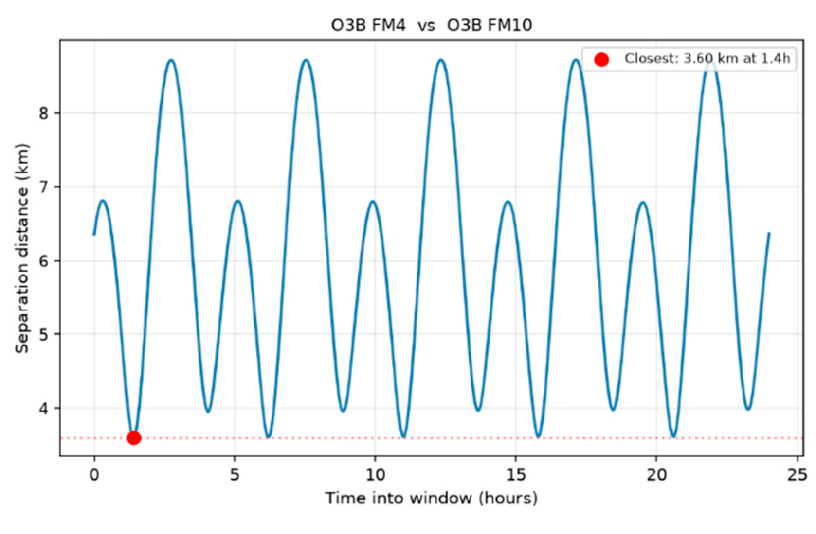
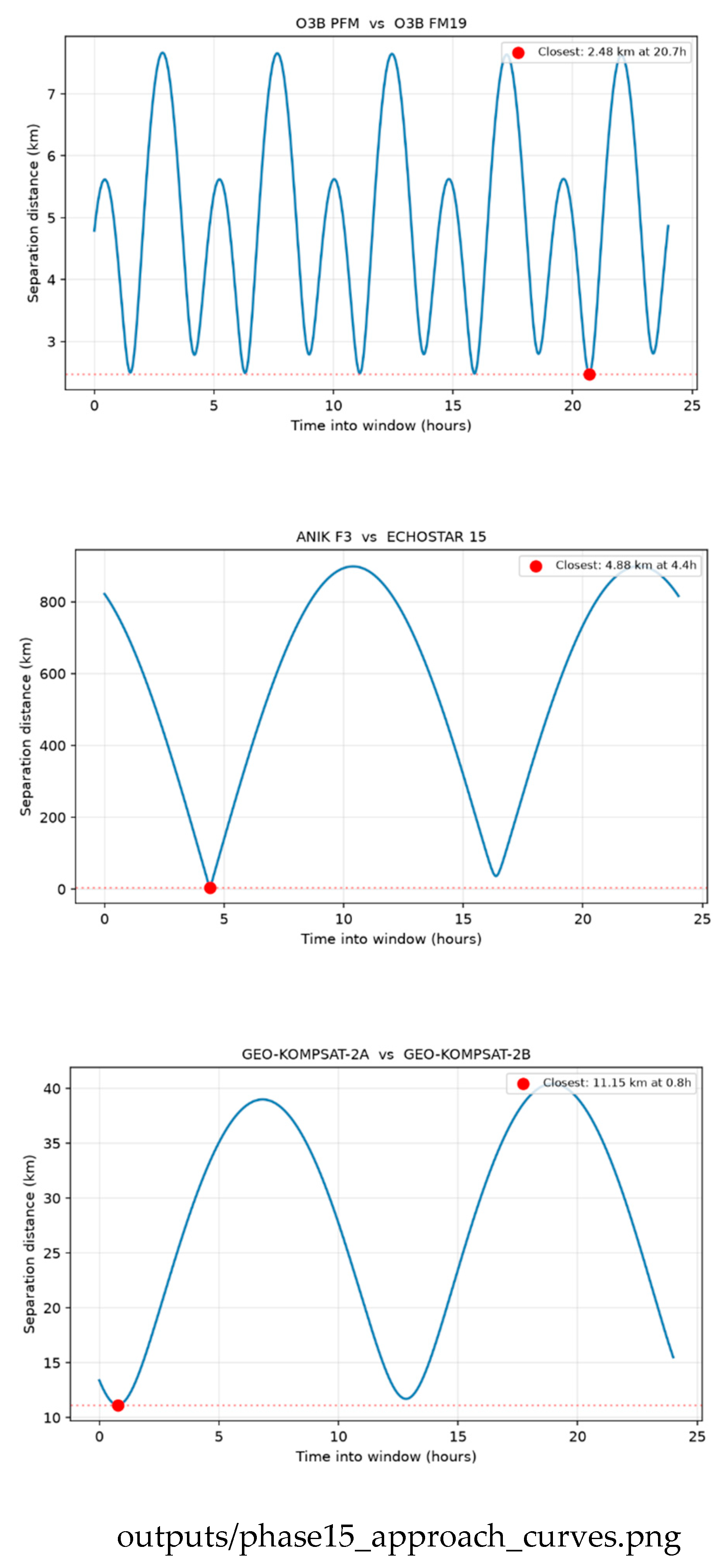
Figure 10.
Active satellites (blue) screened against real debris fragments (red) from the Fengyun-1C, Iridium-33, and Cosmos-1408 events, with the fragment count per source event. Source: github.com/Aditya29072002/Satellite-Conjunction-Assessment — outputs/phase16_debris.png.
Figure 10.
Active satellites (blue) screened against real debris fragments (red) from the Fengyun-1C, Iridium-33, and Cosmos-1408 events, with the fragment count per source event. Source: github.com/Aditya29072002/Satellite-Conjunction-Assessment — outputs/phase16_debris.png.
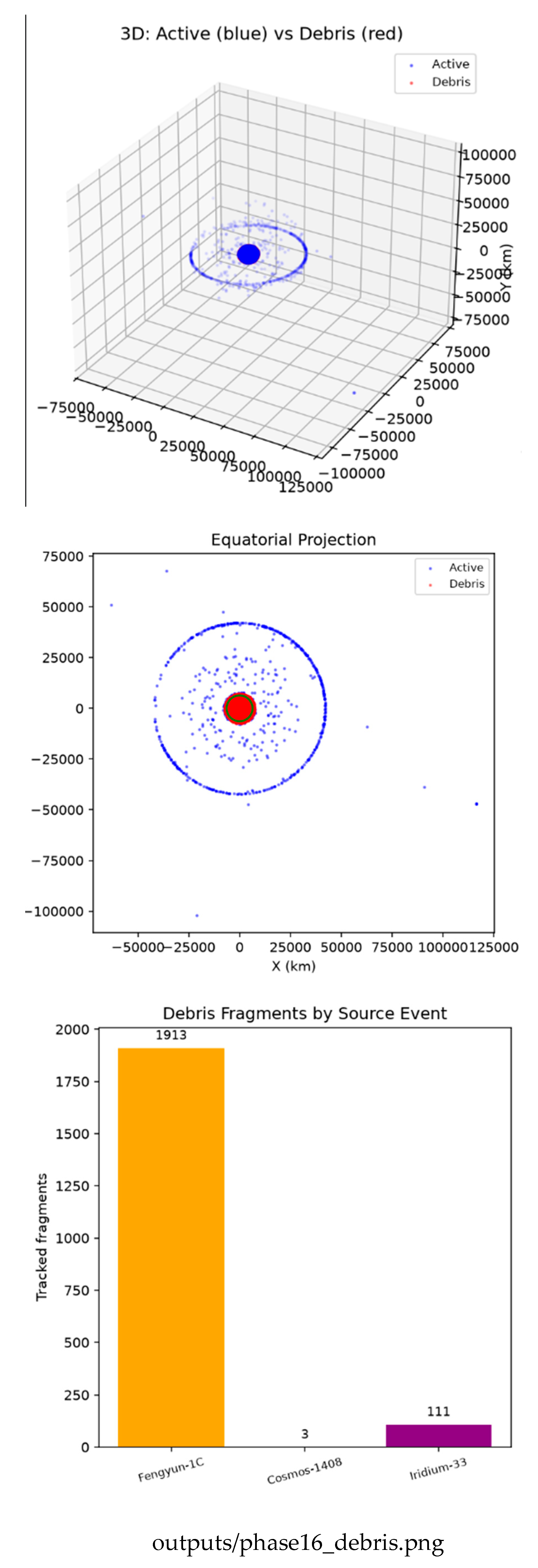

Table 1.
GENUINE DISTINCT-OBJECT CLOSE APPROACHES (24-HOUR WINDOW).
| Object A | Object B | Min Dist. | Time (h) |
|---|---|---|---|
| O3B FM4 | O3B FM10 | 3.59 km | 23.3 |
| MMS 2 | MMS 3 | 8.43 km | 10.7 |
| BADR-5 | ARABSAT-5A | 9.92 km | 17.2 |
| ANIK F3 | ECHOSTAR 15 | 11.48 km | 9.7 |
| GSAT-7 | GSAT-14 | 15.01 km | 20.5 |
Table 2.
STRONG-SCALING PERFORMANCE (REAL 24-HOUR WORKLOAD).
| Cores | Time (s) | Speedup | Effic. (%) |
|---|---|---|---|
| 1 | 1.0821 | 1.00× | 100.0 |
| 2 | 0.5605 | 1.93× | 96.5 |
| 4 | 0.2940 | 3.68× | 92.0 |
| 8 | 0.2476 | 4.37× | 54.6 |
| 16 | 0.2045 | 5.29× | 33.1 |
Table 3.
WEAK-SCALING PERFORMANCE (CONSTANT WORK PER CORE).
| Cores | Total Steps | Time (s) | Effic. (%) |
|---|---|---|---|
| 1 | 30 | 0.4187 | 100.0 |
| 2 | 60 | 0.4256 | 98.4 |
| 4 | 120 | 0.4296 | 97.5 |
| 8 | 240 | 0.7019 | 59.7 |
| 16 | 480 | 1.0780 | 38.8 |
Disclaimer/Publisher’s Note: The statements, opinions and data contained in all publications are solely those of the individual author(s) and contributor(s) and not of MDPI and/or the editor(s). MDPI and/or the editor(s) disclaim responsibility for any injury to people or property resulting from any ideas, methods, instructions or products referred to in the content. |
© 2026 by the authors. Licensee MDPI, Basel, Switzerland. This article is an open access article distributed under the terms and conditions of the Creative Commons Attribution (CC BY) license (http://creativecommons.org/licenses/by/4.0/).
Copyright: This open access article is published under a Creative Commons CC BY 4.0 license, which permit the free download, distribution, and reuse, provided that the author and preprint are cited in any reuse.