

Submitted:
28 September 2026
Posted:
30 September 2026
You are already at the latest version
Abstract
Industrial parks and company growth are vital for urban planning and development. With temporal data collection, mathematical model based growth predictions of industrial parks becomes feasible. In this study, an industrial park Land development Simulation and Company Growth Projections (LSGP) framework is proposed by applying satellite data for land development simulation and social big data for company growth analysis. The cellular automata model is developed to simulate land use development, and the logistic function is applied to set up company growth projection model for selected industrial parks. Results show that the LSGP framework can effectively simulate industrial park land expansion and growth patterns with the following main findings: (1) Underlying land growth follows similar patterns, and key influencing factors are similar, such as traffic convenience, adjacent to urban centers; (2) Company growth pattern follows a logistic growth curve, with each subgroup of companies following the same pattern; (3) Models developed based on a selected industrial park can be transferred to another, i.e., case-based studies can be applied to newly planned industrial parks; (4) The LSGP framework may be further developed to simulate various land use projects and emulate growth patterns for additional areas of interest.
Keywords:
industrial park
; cellular automata
; land use simulation
; company growth
; urban planning
1. Introduction
Industrial parks, as the primary physical carriers of industrial agglomeration and innovation, constitute a representative focal point in the transformation of contemporary urban planning from expansive growth management to the fine-grained regulation of land use structure and spatial quality [1,2]. Their development is characterized by high spatiotemporal heterogeneity, involving not merely simple boundary expansion but also intricate processes of internal textural reorganization, infill development, and infrastructure penetration [3,4]. Traditional planning methodologies, which predominantly rely on static cross-sectional analyses or periodic statistical reports, are insufficient to capture the dynamic interplay between compact, intensive development and peripheral sprawling growth that defines these zones [5]. Consequently, advancing a quantitative understanding of industrial land morphology and constructing an analytical framework capable of precisely mapping land cover transformation trajectories is a foundational step in steering spatial planning from an experience-based practice toward a data-driven, evidence-based science [3,4].
Within the established research domain of land use change, the quantitative characterization of built-up area expansion has long been a core metric for evaluating the coordination of human-land relationships [4,6]. An extensive body of literature has explored conversion mechanisms in heterogeneous suburban or mixed-function areas, yet significant technical hurdles persist in isolating the pure growth signal of construction land within high-standard industrial parks. These zones present unique remote sensing challenges, such as spectral confusion between impervious surfaces including metal factory roofs, and surrounding bare soil or fallow land, which complicates automated classification using standard spectral indices [7]. Furthermore, current analytical practices are frequently constrained by the insufficient granularity of multi-source data fusion and a lack of methodological support for translating long-term spatial distribution sequences into the continuous evolutionary parameters required for predictive modeling [8]. Machine learning classifiers and cellular automata (CA) models have been applied to urban land studies and growth simulation with considerable success [9,10], yet their application to the specific dynamics of industrial park land use remains comparatively underexplored. This technological bottleneck manifests as a critical information deficit for decision-makers, who face substantial lags and scale mismatches when attempting to prospectively delineate the potential footprint of new industrial plots, calculate sustainable development intensity thresholds, or optimize the layout of supporting road networks. Developing forward-looking simulation tools that accommodate complex spatial constraints and integrate multi-dimensional factors is therefore of paramount importance for enhancing the foresight, precision, and implementation feasibility of urban planning [10,11].
The advancement of digital technologies provides means for land use and planning. Remote sensing and satellite technology have greatly enhanced our ability to observe the Earth’s surface on a large scale [12,13] and monitor time-series changes [14,15]. Based on multisource remote sensing data [16], advanced geographic information system (GIS) technologies, and improved artificial intelligence (AI) algorithms, land use and land change have been studied extensively [13,15]. GIS applications with multiple spatial resolutions are available, ranging from coarse resolution to finer resolution, from classical mapping classifiers to advanced convolutional neural network (CNN) algorithms [17,18]. As for algorithms, machine learning algorithms such as random forest (RF) [19,20], classification and regression tree (CART) [21], support vector machine (SVM) [22], etc., are explored for urban land studies. CA models have been widely used to simulate urban growth and land use change [23,24]. These models have been applied to various contexts, such as rural-urban land conversions and urban formation [25,26], demonstrating CA modeling abilities to capture urban growth dynamics and provide helpful planning tools for testing different land development scenarios. The integration of GIS with CA models has been explored to improve the simulation of land use changes and urban development [27,28,29]. These models incorporate high-resolution spatial data to represent land-use change in rural-urban settings and enable detailed analysis of land use changes locally and globally. Computational models have been proposed to link micro-level behavior with macro-level land use dynamics [30]. Applications of related studies in the areas of system dynamics, artificial immune systems, and data mining techniques in combination with CA models have been explored to simulate land-use dynamics, exploring new ways to construct transition rules for geographical CA [31,32,33]. The sensitivity analysis of CA models has also been conducted to assess behavior and the influence of neighborhood size and type on the model’s output [34,35]. In addition, the integration of agent-based, non-linear CA and logistic algorithm has been proposed to improve the simulation accuracy of urban land-use changes and to calibrate CA models based on landscape metrics [36,37,38].
While significant efforts are made globally to study industrial parks planning and management, gaps exist for growth in quantitative analysis and model-based planning for land use and company growth. Because such analysis requires a finer scale of land use data and accumulation of historical data. The following areas require further study: 1) Examine and study land use modeling at industrial park level, where land covered is at a much smaller scale when using mathematic algorithms such as CA; 2) The key objective of developing industrial parks is to foster startup companies and to facilitate growths. Are there underlying growth patterns or principles for such growths, such as the number of companies or other measures? Can such patterns be simulated by setting up mathematical models if they exist? For this study, we explore mathematical models and digital simulations for understanding the fundamental principles and patterns governing the development of industrial parks, focusing on land use dynamics and growth trajectories of companies within industrial parks. The industrial park land development simulation and company growth projections (LSGP) framework is proposed to utilize satellite data for land development simulation and social big data for company growth analysis. The proposed LSGP framework includes two models: 1) The land use model, applying the CA algorithm to simulate land use and development temporally; 2) The company growth model, applying the logistic function to analyze company growth pattern in terms of overall growth and clustering effects for different groups of companies within industrial parks. Industrial parks in Xiamen and Shanghai are selected for developing the models and simulation study. Our findings highlight the underlying growth principles of industrial parks, which are of value in optimizing the planning and development of industrial parks.
The remaining sections of this paper are organized as follows: Section 2 provides an in-depth description of the study area and the data sources. Section 3 outlines the framework of the industrial park LSGP. Section 4 entails methodology through case studies. Section 5 showcases the experimental results and analysis. Section 6 follows with discussions and future work. Section 7 encapsulates the conclusions.
2. Study Area and Datasets
2.1. Study Area
Three industrial parks were selected for this study, two in Xiamen and one in Shanghai. The two industrial parks in Xiamen were chosen because of their locations and environments, while the reason for selecting the industrial park in Shanghai was to find model similarities across regions. Brief descriptions of each industrial park are as follows:
1. The Xiamen Software Park III (Land A) is located north of Jimei District, south of Houxi Town, east of Guankou Town, west of Jimei Cultural and Educational District, facing Xinglin Bay, and adjacent to Yuanbo Garden. It is an essential part of Jimei newly developed new district, as shown in Figure 1 (d). The total planned area is 10 square kilometers, with a building area of 8.6 million square meters. As planned, it can accommodate 2000 companies, amounting to 200,000 employees. The main focus areas are in the following five sectors: Big data and artificial intelligence, Digital creativity, E-commerce, Smart cities and industrial applications, and Mobile Internet.
2. Xiamen Science and Technology Innovation Park (Land B) is located at the junction of Jimei District and Tong’an District with a planned area of 4.9 square kilometers, as shown in Figure 1 (d). It is planned to support the development of the Circum Eastern Sea Area. The functional layout of the industrial park consists of central office areas, research and development (R&D), industrial design centers, software industry areas, and living and supporting areas.
3. Zizhu Industrial Park (Land C) is located southeast of the Minhang District of Shanghai City, is convenient for transportation, and has a planned area of 13 square kilometers. It comprises three parts: University Park, Research and Development Center, and Zizhu Peninsula, as shown in Figure 1 (e). The University Park is located on the campuses of Shanghai Jiaotong University and East China Normal University, promoting cooperation between universities and enterprises. The Zizhu Peninsula is located in the park’s southeast corner, planned for a friendly and convenient large-scale residential community.
2.2. Datasets
We used multisource datasets, mainly categorized into two groups: (1) high-resolution satellite data from Gaofen-7 (GF-7) and (2) social big data collected from publicly available Internet resources and different companies, such as Qichacha and Gaode.
Regarding satellite data, GF-7 satellite images of Xiamen and Shanghai were collected for identification and comparative analysis of developed, undeveloped, and constrained areas in different industrial parks, as shown in Figure 1. The GF-7 satellite provides high-resolution and refined images, with a resolution of 0.65m after true color image fusion [39]. GF-7 also includes high-resolution images in the red, green, blue, infrared, and near-infrared bands. The three-dimensional remote sensing information obtained by GF-7 can extract DEM/DSM and its variation information from different periods [40]. Therefore, the GF-7 images used in this study can provide more on-site information when restoring urban details.
The GF-7 L1A-level data used in this study have undergone sensor-level systemic radiometric and coarse geometric correction. However, standardized preprocessing is still required prior to alteration information extraction. First, the original digital number (DN) values of the imagery are converted to top-of-atmosphere spectral radiance (or TOA reflectance) using onboard calibration coefficients, thereby eliminating sensor gain and offset discrepancies. Subsequently, atmospheric correction is performed using the FLAASH or 6S model to reduce the effects of aerosol scattering and atmospheric absorption, and to retrieve surface true reflectance, ensuring spectral comparability for subsequent band-ratio-based alteration indices. Given that both the forward- and backward-looking cameras of GF-7 employ off-nadir side-looking imaging, topographic relief introduces significant parallax distortions; therefore, orthorectification is conducted based on the RPC model with DEM data for each band to remove topographic and geometric distortions, and to unify all data into a consistent map projection coordinate system (CGCS2000/UTM). To balance spatial detail and spectral information, the 0.8 m panchromatic image and the 3.2 m multispectral images are fused via the Gram–Schmidt (GS) or PANSHARPEN method to generate high-resolution multispectral imagery. Finally, geometric refinement is performed using ground control points (with RMS error controlled within one pixel), followed by registration, mosaicking, color balancing, and vector-boundary clipping of the study area for multiple scenes, with cloud-covered and noisy regions excluded. This yields a GF-7 remote sensing dataset with precise geometry, consistent radiometry, and readiness for direct application in alteration anomaly extraction.
In addition to satellite images, different types of social data, especially companies’ POIs, were collected. The POI data collected from Qichacha contains company information, including name, location coordinates, registration time, company type, etc. Take Xiamen Industrial Parks as an example, 408,358 POIs are retained after performing data cleansing and filtering.
3. Industrial Park Lsgp Framework
The Land Development Simulation and Company Growth Projections (LSGP) framework consists of four modules: Data Model, Land Simulation Model, Company Growth Model, and Visual Analysis Module. The functional diagram is shown in Figure 2, which we will describe in detail next.
3.1. Lsgp Data Model
The LSGP Data Model is based upon the City Meta Unit (CMU) data model developed previously in Xiamen [20], for which satellite and social big data are collected and processed.
3.2. Ca Modeling for Land Development Simulation
CA is a mathematical framework used to model the spatio-temporal behavior of complex systems. In the context of urban land development simulation, CA models simulate the growth and evolution of land use patterns over time.
A commonly used model of constrained CA is selected in this study as a basic framework for urban modeling. The components of constrained CA include transition rules, neighborhood constraints, and stochastic perturbation [35]. These components are combined in a form of Equation (1):
(1)
where is the development probability, Sij represents the transition rules, Cijis the constraint of specific land use, represents the impact of neighborhood configuration, and RA is the stochastic perturbation term reflecting the effect of unconsidered factors (a random number within the range of [0,1)). This article uses 3 x 3 Moore neighborhood formulated as Equation (2):
(2)
where m is the window size, andcon()is a conditional function which returns true if the stateLij is developed land use in neighborhood.
The constraint of land use covers developed, undeveloped, and constrained in our study. Hence, the expression of Cij is as Equation (3), which means the transition from constrained to developed is impossible.
(3)
After obtaining the development probability, the evolution of urban land use during each iteration is completed through the following two steps. First, those available pixels (undeveloped) are sorted in a descending sequence based on. Second, pixels with higher development probabilities will be converted to developed preferentially. To ensure the simulated urban land use matches the observed, the number of converted pixels during each iteration is determined using a linear allocation scheme, which can be expressed as Equation (4).
(4)
where Per denotes the number of converted pixels during each iteration, D is the total conversion number of urban land use during the entire simulation phase, which is determined from the observed land use at two different phases, and K is the total number of iterations.
3.3. Model Parameter Setup
3.3.1. Transition Rules of Ca Model
Transition rules calculation is very important in urban CA modeling. Calibrating processes can be achieved via various AI algorithms based on historical data. Performances of obtained transition rules depends on the quantity and quality of training samples, and the selected mathematical models. This study uses the Logistic Regression (LR) model to estimate probability of each pixel in the selected area [35], which can be expressed as Equations (5) and (6) jointly:
z = b0 + b1x1 + b2x2+…+bnxn (5)
where Sij is the probability derived from LR model, [x1,x2,…,xn] are independent variables related to land development, and [b1,b2,…,bn] are regressed coefficients for different variables, b0is a constant.
3.3.2. Logistic Model for Company Growth Model
For projecting company growth in an industrial park, the Logistic Growth (LG) model is used to emulate the changing trends of company numbers, which can be expressed as Equation (7):
(7)
where y represents the total number of companies, t represents the feature variable (time period), a is the initial value, b is the upper limit of the logistic curve based on the zero baseline (a+b is the final upper asymptote of the LG model, which together reflect the saturation level of number of companies in the industrial park), c is the slope of the logistic curve (reflecting the growth rate), d is the inflection point. Parameters a and b are constants, while c and d are obtained from model training.
4. Lsgp-Based Land Use Simulation and Company Growth Projection for Xiamen and Shanghai Industrial Parks
Based on the LSGP framework, we set up the LSGP data model for land use simulation and company growth projections. For the land simulation, both LR and CA models are applied. The land grid is set up for Land A, the grid size is 5 meters x 5 meters. We have used Land B and Land C as case-based references for model parameter acquisition. For company growth emulation, we set up an LG model each for the three selected land areas. The inspiration for using LG model is based on our observations of company growth patterns for the selected industrial parks, which was verified and described by the proposed model in section 5. The implementation of the proposed method is shown in Figure 3.
4.1. Data Preparation
4.1.1. Land Use Data Processing
We collect labeling data for land use of Land A and Land B in 2010 and 2017 and for Land C in 2002 and 2022 separately. Each land has its geographic features such as main highway, main road, relief road, dem, slope, etc. Through the unified map projection coordinate system (CGCS2000/UTM), these image data are preprocessed to obtain the label data and feature data with a pixel size of 5m * 5m and resolution of 618 * 1556 (Land A), 719 * 673 (Land B), and 790 * 1182 (Land C), respectively. Taking Land A as an example, the data processing steps are as follows:
(1) Data annotation
Annotating the acquired remote sensing images for the first and second periods manually classified into three different areas: a) Developed areas: schools, buildings, villages, impervious surface, public garden, roads, and factories; b) Undeveloped areas: farmland, bare land, grassland, wasteland, and changed lakes; c) Constrained areas: rivers, unchanged lakes, forests, railways, and mountains.
(2) Label processing
By comparing the annotated land use data for each of the two periods, the classification labels for each pixel are obtained [25], as shown in Figure 4. Then sampling pixels from the developed area (labeled as 1) and the undeveloped area (marked as 0) to obtain training samples and label data.
(3) Feature processing
By locating geographical feature points near the industrial park, such as road intersections, subway stations, market centers, etc., the feature values of each pixel (the distance to these feature points) are calculated to obtain feature maps of the park. Extracting the corresponding feature values of each sample pixel from the feature maps and integrating them with the label data to form a complete training sample dataset. The description of the features is shown in Table 1 below.
4.1.2. Company Data Processing
The data processing steps for company growth are as follows:
(1) Retrieve the company data of Xiamen and Shanghai from publicly available Internet resources through Qichacha, including the basic information of each company, such as name, address, registration time, type, etc.
(2) Convert company addresses into latitude and longitude coordinates by Gaode API.
(3) Use ArcGIS software to project company POIs according to longitude and latitude coordinates and perform intersection processing with the shape file of the industrial park to obtain companies inside each park.
(4) Conduct statistical analysis of company data in each park yearly to get the number of companies and their cumulative quantity for each year.
(5) Further preprocess the statistical result to obtain the sample data for LG modeling.
By plotting the growth curves, we observed that the company growth follows a logistic pattern, which led us to adopt the LG model.
4.2. Ca Modeling for Land Use Simulation
As described in section 4.1.1, 1,000 samples are randomly sampled for Land A, Land B, and Land C, separately, including 500 positive samples and 500 negative samples, each containing 9 feature values (7 for Land C). Manual validations are conducted for Land A, removing the incorrectly labeled samples and retaining 837 samples, namely 417 positive and 420 negative samples. By splitting the training and testing data, 737 training samples and 100 testing samples are obtained for Land A, while 900 training samples and 100 testing samples are obtained for Land B and Land C. The steps to simulate land development using the CA algorithm are as follows:
(1) Train the LR model using the training set of Land A, and evaluate the accuracy of the model using the testing set.
(2) Extract the feature value combination of each pixel in Land A through the feature maps and use the LR model to predict each pixel to obtain the static development probability of Land A.
(3) By comparing the land use data of Land A in 2010 and 2017, the total number of converted pixels in the developed area is 67,713, which determined that the average number of converted pixels per iteration is 9,673.
(4) The number of iterations is set to 7. Before the first iteration, 5,000 pixels with the highest static development probability are selected, and land development simulation is conducted using the CA algorithm described in Section 3.2. In each iteration, the 9,673 pixels with the highest dynamic development probability in the undeveloped area will be converted into developed areas.
(5) Compare the predicted results of each iteration with the actual land use results in 2017, calculate the overall accuracy (OA) and figure of merit (FOM) [4] indicators, and evaluate the effectiveness of CA simulation, which can be expressed as Equations (8) and (9) respectively.
where Mii is the number of correctly classified pixels on the diagonal of the confusion matrix (consists of real and predicted land use categories), n denotes the number of land use categories. The denominator represents the total number of valid pixels.
where is an area of error due to real change pixels predicted as unchanged, is an area of accuracy due to correctly predicted change pixels, is an area of error due to real change pixels predicted with incorrect categories, and is an area of error due to unchanged pixels incorrectly predicted as changed.
(6) Similarly, train the LR models of Land B and Land C, and transfer them to Land A for land development simulation by replacing the LR model of Land A. Repeat steps (2) - (5), then compare the simulation results and verify the feasibility of model transfer from different lands.
4.3. Logistic Model to Emulate Company Growth
As described in Section 4.1.2, we obtained 4,001 companies for Land A, 621 companies for Land B, and 3,726 companies for Land C. The starting time of modeling is the year when the industry park began to develop. Land A, B, and C are all in 2014. Seven regression sample data are obtained respectively. The steps to emulate company growth using the LG model are as follows:
(1) Determine the values of constants a and b in the LG model based on statistical company data.
(2) Take the company numbers as the target y and the establishment period of the industrial park as the feature t (values are 0-6). According to equation (7), if z' = −c × (t − d), then z' = ln[y'/(1 − y')], where y' is the normalized value of y, which transforms nonlinear data into linear data.
(3) Train and test z' using the linear regression algorithm (5 training samples and 2 test samples), and use the mean absolute error (MAE) and coefficient of determination (R2) as evaluation indicators, then obtain parameter values of c and d.
(4) By substituting the values of a, b, c, and d into the LG model, the emulation data and LG curve of companies for different parks can be obtained.
5. Results and Analysis
5.1. Industrial Park Land Simulation
5.1.1. Ca Modeling Based Land Simulation
For Land A, the accuracy of the trained LR model on the testing set is 79.00%, and the regression coefficients are [-0.2929, -0.3695, -0.0201, -0.2110, 0.1571, -0.6468, 0.1887, -0.6157, 0.0678], namely
According to the method described in Section 4.2, the land development simulation result for Land A based on CA algorithm is shown in Figure 5 below.
The changing curves of OA and FOM for different iterations are shown in Figure 6 below. By obtaining the label values between the map generated by each iteration and the actual land use map in 2017, the OA can be calculated using Equation (8), in which the confusion matrix consists of simulated and actual land use categories, including developed, undeveloped and constrained areas. By comparing the label values of 9,673 pixels converted in each iteration with the values of the corresponding pixels in the actual map, the FOM can be calculated using Equation (9).
We observe that the average OA and FOM in 7 iterations are 0.9059 and 0.2892, respectively; the OA and FOM of final simulation result in 2017 are 0.8916 and 0.2390, respectively.
5.1.2. Model Transfer Based Land Simulation
For Land B, the accuracy of the trained LR model on the testing set is 74.00%, and the regression coefficients are [0.5012, -0.8220, 0.1609, 0.0803, -0.0128, 0.0377, -0.1427, -0.0968, -0.3063], namely
For Land C, the accuracy of the trained LR model on the testing set is 73.00%, and the regression coefficients are [-0.4119, -0.3513, -0.0518, 0.0889, 0.1059, -0.3936, -0.3117], namely
According to the method described in Section 4.2, transfer the LR model of Land B to Land A, and then also use the CA algorithm to simulate the land development of Land A. The result is shown in Figure 7.
The changing curves of OA and FOM for different iterations are shown in Figure 8 below. As for the LR Model transfer of Land B, the average OA and FOM in 7 iterations are 0.8993 and 0.2277, respectively; the OA and FOM of final simulation result in 2017 are 0.8830 and 0.2253, respectively.
Similarly, transfer the LR model of Land C to Land A, and then use the CA algorithm to simulate the land development of Land A. The result is shown in Figure 9.
The changing curves of OA and FOM for different iterations are shown in Figure 10 below. As for the LR Model transfer of Land C, the average OA and FOM in 7 iterations are 0.9055 and 0.2911, respectively; the OA and FOM of final simulation result in 2017 are 0.8919 and 0.2445, respectively.
The comparison of the average OA and FOM values of the land development simulation results for Land A based on the LR models of Land A, B, and C is shown in Table 2 below.
5.1.3. Land Simulation: Prediction for Future Growth
By comparing the land use data of Land A from 2017 and 2023, the total number of converted pixels in the developed area is 106,730, which determines that the average number of converted pixels per iteration during the period is 17,788.
As stated in Section 2.1, it is known that the total planned area of Land A is 10 square kilometers, the planned building area is 8.6 million square meters, and the planned plot ratio is 4. The land development area can be calculated based on the building area and plot ratio through the following formula. By comparing with the land development area in 2023, the number of converted pixels for each subsequent year can be obtained. It is known that the building area in 2023 is 4.8 million square meters. Assuming that Land A will be fully developed by 2035, the calculation process is as follows:
(1) Assumed land development area in 2035 = Building area in 2035 / plot ratio = 8.6 million square meters/4=2.15 million square meters
(2) Actual land development area in 2023 = Building area in 2023 / plot ratio = 4.8 million square meters/4=1.2 million square meters
(3) Subsequent annual converted pixels = ((Assumed land development area in 2035 - Actual land development area in 2023)/Pixel area) / Duration years = ((2.15 million square meters -1.2 million square meters)/25 square meters)/12=3,167
Based on the result in Section 5.1.1, the CA algorithm is further applied to iterate to predict future land development of Land A. The prediction result is shown in Figure 11 (9,673 converted pixels in each iteration from 2010 to 2017, 17,788 converted pixels in each iteration from 2018 to 2023, and 3,167 converted pixels in each iteration from 2024 to 2035).
5.2. Industrial Park Growth Emulation
5.2.1. Company Growth Emulation for Land A
As described in Section 4.3, LG modeling is conducted on the company growth data in Land A, and the parameters a=716, b=3,285, c=0.9127, d=3.6203 are obtained. The MAE on the testing set is 36.2903, and the R2 score is 0.9983. The emulation results are shown in Figure 12.
The companies in Land A are divided into six categories according to their respective industries: software industry, technology service industry, business service industry, wholesale and retail industry, manufacturing industry, and others. In the same way, statistical processing and LG modeling are conducted for each sector. The parameters of the LG model for different industries are shown in Table 3, and the emulation results are shown in Figure 13.
5.2.2. Model Transfer Based Company Growth Emulation
Similarly, LG modeling was conducted on the company growth data in Land B and C, and the LG model parameters are obtained as shown in Table 4. The emulation results are shown in Figure 14.
Through comparison, we can find that the emulation results between Land B, C, and A have some similar trends. Therefore, the LG models of these two lands can be transferred to Land A, where the parameter values of c and d in Land A are replaced with the corresponding values in Land B and C. The parameter values of a and b are constants and remain unchanged. The emulation results are shown in Figure 15.
5.2.3. Company Growth Prediction for Future
We can emulate the future company growth based on land development; that is, the parameters of a and c in the LG model remain unchanged, while the parameters of b and d will be modified according to the plan specified. Assuming that the land development of Land A reaches saturation in 2024, the company growth lags by four years and reaches saturation in 2028. The company’s growth starts in 2014, so the inflection point is in 2021, and the actual company numbers in 2021 are 4,737. Equation (7) shows that the parameters d=7 and b=8,042 can be obtained. Substituting them into the LG model of Land A, as described in Section 5.2.1, the emulation result of subsequent company growth for Land A is shown in Figure 16 (a).
Similarly, Land B’s land development reached saturation in 2020, and the company growth reached saturation in 2024. The company’s growth starts in 2014, so the inflection point is in 2019, and the actual company numbers in 2019 is 525. Therefore, the parameters d=5, b=780 can be obtained. Substituting them into the LG model of Land B described in Section 5.2.2, the emulation result of subsequent company growth for Land B is shown in Figure 16 (b).
Similarly, assuming that the land development of Land C reaches saturation in 2024, and the company’s growth reaches saturation in 2028, The company growth starts in 2014, so the inflection point is in 2021, and the actual company numbers in 2021 is 4,301. Therefore, the parameters d=7, b=7,096 can be obtained. Substituting them into the LG model of Land C described in Section 5.2.2, the emulation result of subsequent company growth for Land C is shown in Figure 16 (c).
5.2.4. Land Development Change and Company Growth
The actual land development areas of Land A, B and C per year are obtained by manually labeling the satellite images. By comparing with the emulation results of company growth, the relationships between land development change and company growth are obtained, as shown in Figure 17.
6. Discussion
6.1. Industrial Park Land Simulation Analysis
From the regression coefficients of the LR model in different lands, it can be found that the essential features of land development simulation in Land A are dem, main road, bridge in the island, and main highway. The important features in Land B are the bridge in island, the main highway, and the relief road. The important features in Land C are the main highway, main road, market and relief road. We observe differences and similarities in the important features of land development simulation in different land areas. The features with high contributions mainly include main highway, main road, relief road, and bridge in island. Since Land C is located in Shanghai, and the geographical characteristics of Shanghai and Xiamen are different, i.e., there are no cross-sea bridges in Shanghai. Therefore, when comparing Land C to Land A, Land C does not have the features of bridge in and out islands. Therefore, when transferring the LR model of Land C to Land A for land development probability prediction, it is also necessary to remove these two features of Land A to ensure the effectiveness and accuracy of the model transfer.
From the land development simulation results in 2017 and OA and FOM indicators generated by CA iteration using different LR models, as shown in Table 2, the OA and FOM based on the model of Land B are slightly lower than the model of Land A, while the simulation results based on the model of Land C and Land A are relatively close. The results support the feasibility of transfer learning and land development simulation using the models in different lands. In the future, this method can be extended by transferring existing models to new land areas and simulating the land development situation of the new land areas.
This study also attempts to determine the number of converted pixels for future land development simulation based on the total planned building area of Land A, which demonstrates that the CA algorithm can be applied to continue the iteration based on the result shown in Figure 5, so as to predict the future land development simulation results.
6.2. Industrial Park Company Growth Emulation Analysis
By emulating the company growth in Land A, B and C, and transfer the LG models of Land B and C to Land A (by modifying parameters c and d), as shown in Figure 15, it can be found that compared to the LG model of Land A, the parameters c and d in LG model of Land B are larger and smaller, respectively, while the parameters c and d in LG model of Land C are smaller, but the inflection point d is closer. The company growth patterns in Land C and Land A are more similar. In general, the emulation results based on the transfer models and the model of Land A have small errors and are similar to a certain extent, which proves the feasibility of transfer learning of company growth model for different industrial park land areas.
For the same land space, different types of companies exhibit the same overall LG growth patterns, but differencing in time and growth numbers, which merits further studies. Based on the company growth emulation results in different industries of Land A, as shown in Figure 13, the following conclusions can be drawn: the industries with larger parameter value of a+b (company capacity) are software industry, wholesale and retail industry, and other industries; the industries with larger parameter value of c (growth rate) are business services industry, wholesale and retail industry, and technology services industry; the industries with smaller parameter value of d (inflection point) are technology services industry, manufacturing industry, and software industry. After further analysis, it can be found that there are some internal patterns in the industry development of Land A: (1) The relationship between the software industry, technology service industry, and business service industry: The technology service industry develops first, providing infrastructure for the software industry. After the software industry reaches a specific scale, then the business service industry begins to grow, providing business services such as marketing, financial management, and investment management for the software industry; (2) The development of wholesale and retail industry is relatively good, second only to the software industry, which should be related to the policies introduced in Xiamen in recent years to promote the development of e-commerce; (3) The manufacturing industry and other industries are not the dominant sectors in Land A, and their growth is relatively less prominent.
The future company growth can be emulated based on land development changes. By comparing the actual land development change area of these lands with the company growth simulation results, as shown in Figure 17, it is concluded that both the land development and company growth exhibit a logistic pattern growth curve, and the company growth curves lags behind the land development change curve generally. This phenomenon is in line with the reality.
6.3. Limitations and Future Research
In terms of land development simulation, due to the exponential curve variation of urban development, the converted number of CA models in different years during the land development process may be different. In the future, the land use data during the iteration period can be annotated to obtain the actual changed area and converted numbers of the developed zone each year. Then, the converted number during the CA iteration process can be continuously adjusted based on the actual changes, so the simulation results are closer to the real land development situation. Besides, we will attempt to conduct spatially independent validation of the model, such as spatial blocks or geographically separated sampling areas, in order to avoid possible accuracy inflation caused by adjacent pixels. In addition, regarding the transfer rules of CA, this study only uses the LR model. In the future, other algorithms such as CART and RF can be attempted to explore the effectiveness and applicability of machine learning algorithms in land development simulation further.
In terms of company growth, due to difficulties in obtaining data and limitations in data sources , this study only emulates the company numbers for 7 years and predicts their subsequent growth trends. In the future, we will conduct temporal validation by collecting real data from subsequent years, and evaluate the uncertainty of the LG model’s predictive performance. Then, efforts can be made to emulate additional dimensions of industrial data or indicators, such as GDP, number of employees, etc. LG modeling analysis can be conducted to fully illustrate the influencing factors and development patterns of industrial growth. Besides, as the number of company grows, so-called “unicorn” companies may excel, which in turn would impact the ecosystem, which often happens among the leading innovating areas worldwide [41,42]. In addition, for this study, we have assumed the land space of a selected industrial park is constructed as planned and fully utilized, which is true in an uptick under normal development phase. We hypothesize that it will be interesting to study and simulate when land space is not fully used; therefore, company growth may be a plateau, or even decline.
The land simulation and company growth in this study mainly focus on Land A. At the same time, the models of Land B and C are transferred to Land A for comparative analysis to verify the feasibility of model transfer learning between different lands. In the future, we can refer to the practice of Land A, conduct more in-depth research on Land B and C, and apply the proposed method to additional industrial parks, as well as urbanization predictions based on township development, to further demonstrate the general regularity of industrial park development and the widespread applicability of this study.
7. Conclusions
To effectively plan and develop industrial parks, it is essential to understand thoroughly the fundamental principles and growth dynamics underlying industrial park practices. By harnessing advanced digital technologies, such as high-resolution satellite imagery and accumulating historical data, it becomes feasible to create mathematical models that simulate the growth of industrial parks with enhanced precision at finer scales. In this study, we develop an industrial park Land development Simulation and Company Growth Projections (LSGP) framework by setting up CA and logistic function models. By applying the LSGP framework to industrial parks in Xiamen and Shanghai, we conclude that the LSGP framework is highly effective in simulating industrial park land expansion and company growth pattern. Benefiting from state-of-the-art remote sensing and big data technologies, the study contributes to filling the gap in both industrial park land simulation and company growth patterns in finer scales. First, land use across for industrial parks follows similar patterns. Key factors influencing land use are similar such as traffic convenience, adjacent to key centers etc. Secondly, company growth pattern within an industrial park follows logistic function curve, with each subgroup of companies also following similar pattern. Thirdly, models developed in one industrial park can be transferred to another, i.e., case-based studies can be applied to newly planned industrial parks. These findings provide insights into optimizing planning and design of the industrial parks, and highlights the underlying growth principles of industrial parks. The proposed LSGP framework may be further developed to simulate various land use projects and emulate growth patterns for newly selected criteria.
Author Contributions
Conceptualization, X.W.; methodology, X.W. and XC.L.; formal analysis, X.W., XC.L., XY.L. and B.C.; writing—original draft preparation, X.W., XY.L. and K.L.; writing—review and editing, XC.L., B.C. and P.G.; software, XC.L., XY.L. and K.L.; investigation, X.W., XC.L. and B.C.; resources, X.W. and P.G.; data curation, XY.L., B.C. and K.L.; visualization, X.W., XY.L. and K.L.; supervision, X.W.; funding acquisition, P.G. and X.W. All authors have read and agreed to the published version of the manuscript.
Funding
This research was funded by City Digital Appraisel research project and High-resolution GIS Study for Urban Management Phase II project established by Ministry of Housing and Urban Rural Development of the People’s Republic of China.
Institutional Review Board Statement
Not applicable.
Informed Consent Statement
Not applicable.
Data Availability Statement
The data presented in this study are available on request from the corresponding author. The data are not publicly available due to privacy.
Acknowledgments
This research was supported by Department of Automation, AI for Earth Laboratory, Cross-strait Tsinghua Research Institute, Tsinghua University. We express our appreciation for Professor Jun Li for his guidance for modeling study, and our colleague Gang Yin in the laboratory for his support of field inspection and software preparation.
Conflicts of Interest
The authors declare no conflict of interest.
References
- Long, H.; Qu, Y.; Tu, S.; Zhang, Y.; Jiang, Y. Development of land use transitions research in China. J. Geogr. Sci. 2020, 30(7), 1195–1214. [Google Scholar] [CrossRef]
- Fan, P.; Yue, W.; Zhang, J.; Huang, H.; Messina, J.; et al. The spatial restructuring and determinants of industrial landscape in a mega city under rapid urbanization. Habitat Int. 2020, 95, 102099. [Google Scholar] [CrossRef]
- Seto, K.C.; Güneralp, B.; Hutyra, L. R. Global forecasts of urban expansion to 2030 and direct impacts on biodiversity and carbon pools. Proc. Natl. Acad. Sci. 2012, 109(40), 16083–16088. [Google Scholar] [CrossRef] [PubMed]
- Liu, X.; Liang, X.; Li, X.; Xu, X.; Ou, J.; et al. A future land use simulation model (FLUS) for simulating multiple land use scenarios by coupling human and natural effects. Landsc. Urban Plan. 2017, 168, 94–116. [Google Scholar] [CrossRef]
- Gao, J.; O’Neill, B.C. Mapping global urban land for the 21st century with data-driven simulations and Shared Socioeconomic Pathways. Nat. Commun. 2020, 11, 2302. [Google Scholar] [CrossRef] [PubMed]
- Verburg, P.H.; Soepboer, W.; Veldkamp, A. Modeling the spatial dynamics of regional land use: the CLUE-S model. Ecol. Model. 2002, 154(1-2), 101–118. [Google Scholar]
- Amine, J.; Mohcine, C.; Jaouad, E.; Soufiane, H.; Abdessamad, J. A new index for extracting built-up land features using Landsat satellite imagery. E3S Web Conf. 2025, 607, 03005. [Google Scholar] [CrossRef]
- Clarke, K. C.; Hoppen, S.; Gaydos, L. A self-modifying cellular automaton model of historical urbanization in the San Francisco Bay area. Environ. Plan. B 1997, 24(2), 247–261. [Google Scholar] [CrossRef]
- Breiman, L. Random forests. Mach. Learn. 2001, 45(1), 5–32. [Google Scholar] [CrossRef]
- Batty, M.; Xie, Y. Modeling inside GIS: Part 2—Selecting and calibrating urban models using ARC/INFO. Int. J. Geogr. Inf. Syst. 1994, 8(5), 451–470. [Google Scholar] [CrossRef]
- Verburg, P.; Nijs, T.; Eck, J.; Visser, H.; Jong, K. A method to analyse neighbourhood characteristics of land use patterns. Comput. Environ. Urban Syst. 2004, 28(6), 667–690. [Google Scholar] [CrossRef]
- Yu, L.; Shi, Y.; Gong, P. Land cover mapping and data availability in critical terrestrial ecoregions: A global perspective with Landsat thematic mapper and enhanced thematic mapper plus data. Biol. Conserv. 2015, 190, 34–42. [Google Scholar] [CrossRef]
- Chen, J.; Chen, J.; Liao, A.; Cao, X.; Chen, L.; et al. Global land cover mapping at 30 m resolution: A POK-based operational approach. Isprs J. Photogramm. Remote Sens. 2015, 103, 7–27. [Google Scholar] [CrossRef]
- Yu, L.; Wang, J.; Gong, P. Improving 30 m global land-cover map FROM-GLC with time series MODIS and auxiliary data sets: A segmentation-based approach. Int. J. Remote Sens. 2013, 34, 5851–5867. [Google Scholar] [CrossRef]
- Gong, P.; Wang, J.; Yu, L.; Zhao, Y.; Zhao, Y.; et al. Finer resolution observation and monitoring of global land cover: First mapping results with Landsat TM and ETM+ data. Int. J. Remote Sens. 2012, 34, 2607–2654. [Google Scholar] [CrossRef]
- Jia, W.; Pei, T.; Lei, K. Research on Land Use Planning Based on Multisource Remote Sensing Data. In Computational Intelligence and Neuroscience; 2022. [Google Scholar]
- Chen, B.; Xu, B.; Gong, P. Mapping essential urban land use categories (EULUC) using geospatial big data: Progress, challenges, and opportunities. Big Earth Data 2021, 5(3), 410–441. [Google Scholar] [CrossRef]
- H. N. M.; V. P.; D. Mahesh, S. M.; K.; G, H. S.; et al. LULC Classification Using Deep Convolution Neural Networks for Change Detection Analysis. Int. J. Environ. Sustain. Dev. 2026, 25, 1–2. [Google Scholar] [CrossRef]
- Amini, S.; Saber, M.; Rabiei-Dastjerdi, H.; Homayouni, S. Urban Land Use and Land Cover Change Analysis Using Random Forest Classification of Landsat Time Series. Remote. Sens. 2022, 14, 2654. [Google Scholar] [CrossRef]
- Wang, X.; Chen, B.; Li, X.; Zhang, Y.; Ling, X.; et al. Grid-Based Essential Urban Land Use Classification: A Data and Model Driven Mapping Framework in Xiamen City. Remote Sens. 2022, 14(23). [Google Scholar] [CrossRef]
- Yao, Y.; Li, J.; Zhang, X.; Duan, P.; Li, S.; et al. Investigation on the Expansion of Urban Construction Land Use Based on the CART-CA Model. ISPRS Int. J. Geo Inf. 2017, 6, 149. [Google Scholar] [CrossRef]
- Swetanisha, S.; Panda, A.R.; Behera, D.K. Land use/land cover classification using machine learning models. Int. J. Electr. Comput. Eng. (IJECE) 2022, 12(2). [Google Scholar] [CrossRef]
- Pinto, N.; Antunes, A.P. A Cellular Automata Model Based on Irregular Cells: Application to Small Urban Areas. Environ. Plan. B Plan. Des. 2010, 37, 1095–1114. [Google Scholar] [CrossRef]
- Liu, Y.; Phinn, S.R. Modelling urban development with cellular automata incorporating fuzzy-set approaches. Comput. Environ. Urban Syst. 2003, 27, 637–658. [Google Scholar] [CrossRef]
- Wu, F. Calibration of stochastic cellular automata: the application to rural-urban land conversions. Int. J. Geogr. Inf. Sci. 2002, 16, 795–818. [Google Scholar] [CrossRef]
- Li, X.; Yeh, A.G. Neural-network-based cellular automata for simulating multiple land use changes using GIS. Int. J. Geogr. Inf. Sci. 2002, 16, 323–343. [Google Scholar] [CrossRef]
- Li, X.; Yeh, A.G. Modelling sustainable urban development by the integration of constrained cellular automata and GIS. Int. J. Geogr. Inf. Sci. 2000, 14, 131–152. [Google Scholar] [CrossRef]
- Stevens, D.; Dragićević, S. A GIS-Based Irregular Cellular Automata Model of Land-Use Change. Environ. Plan. B Plan. Des. 2007, 34, 708–724. [Google Scholar] [CrossRef]
- Shubham, B.; Neerav, S.; Munizzah, S.; Kavita, R. D. G.; S. Predictive Modeling of Land Cover Changes in Round-1 Smart Cities of India Using Cellular Automata and GIS. Discov. Cities 2025, 2(1), 1–25. [Google Scholar] [CrossRef]
- Irwin, E.G. New Directions for Urban Economic Models of Land Use Change: Incorporating Spatial Dynamics and Heterogeneity. In ERN: Urban Economics & Public Policy (Topic); 2010. [Google Scholar]
- He, C.; Yuanyuan, Z.; Tian, J.; Shi, P. Modeling the urban landscape dynamics in a megalopolitan cluster area by incorporating a gravitational field model with cellular automata. Landsc. Urban Plan. 2013, 113, 78–89. [Google Scholar] [CrossRef]
- Liu, X.; Li, X.; Shi, X.; Zhang, X.; Chen, Y. Simulating land-use dynamics under planning policies by integrating artificial immune systems with cellular automata. Int. J. Geogr. Inf. Sci. 2010, 24, 783–802. [Google Scholar] [CrossRef]
- Li, X.; Yeh, A.G. Data mining of cellular automata’s transition rules. Int. J. Geogr. Inf. Sci. 2004, 18, 723–744. [Google Scholar] [CrossRef]
- Kocabas, V.; Dragićević, S. Assessing cellular automata model behaviour using a sensitivity analysis approach. Comput. Environ. Urban Syst. 2006, 30, 921–953. [Google Scholar] [CrossRef]
- Li, X.; Liu, X.; Yu, L. A systematic sensitivity analysis of constrained cellular automata model for urban growth simulation based on different transition rules. Int. J. Geogr. Inf. Sci. 2014, 28, 1317–1335. [Google Scholar] [CrossRef]
- Zhao, L.; Peng, Z. LandSys: an agent-based Cellular Automata model of land use change developed for transportation analysis. J. Transp. Geogr. 2012, 25, 35–49. [Google Scholar] [CrossRef]
- Shi, W.; Pang, M.Y. Development of Voronoi-based cellular automata -an integrated dynamic model for Geographical Information Systems. Int. J. Geogr. Inf. Sci. 2000, 14, 455–474. [Google Scholar] [CrossRef]
- Chen, Y.; Li, X.; Liu, X.; Ai, B. Modeling urban land-use dynamics in a fast developing city using the modified logistic cellular automaton with a patch-based simulation strategy. Int. J. Geogr. Inf. Sci. 2014, 28, 234–255. [Google Scholar] [CrossRef]
- d’Angelo, P.; Tian, J. Geometric Evaluation of Gaofen-7 Stereo Data. ISPRS Ann. Photogramm. Remote Sens. Spat. Inf. Sci. 2023, 10-1, 805–811. [Google Scholar] [CrossRef]
- Xie, J.; Huang, G.; Liu, R.; Zhao, C.; Dai, J.; et al. Design and Data Processing of China’s First Spaceborne Laser Altimeter System for Earth Observation: GaoFen-7. IEEE J. Sel. Top. Appl. Earth Obs. Remote Sens. 2020, 13, 1034–1044. [Google Scholar] [CrossRef]
- Adams, S.B. From orchards to chips: Silicon Valley’s evolving entrepreneurial ecosystem. Entrep. Reg. Dev. 2021, 33, 15–35. [Google Scholar] [CrossRef]
- Hogarth, S. Valley of the unicorns: consumer genomics, venture capital and digital disruption. New Genet. Soc. 2017, 36, 250–272. [Google Scholar] [CrossRef]
Figure 1.
Study areas: (a) Industrial parks location; (b) Land A & Land B located in Xiamen; (c) Land C located in Shanghai; (d) Zoomed-in area of graph (b); and (e) Zoomed-in area of graph (c).
Figure 1.
Study areas: (a) Industrial parks location; (b) Land A & Land B located in Xiamen; (c) Land C located in Shanghai; (d) Zoomed-in area of graph (b); and (e) Zoomed-in area of graph (c).
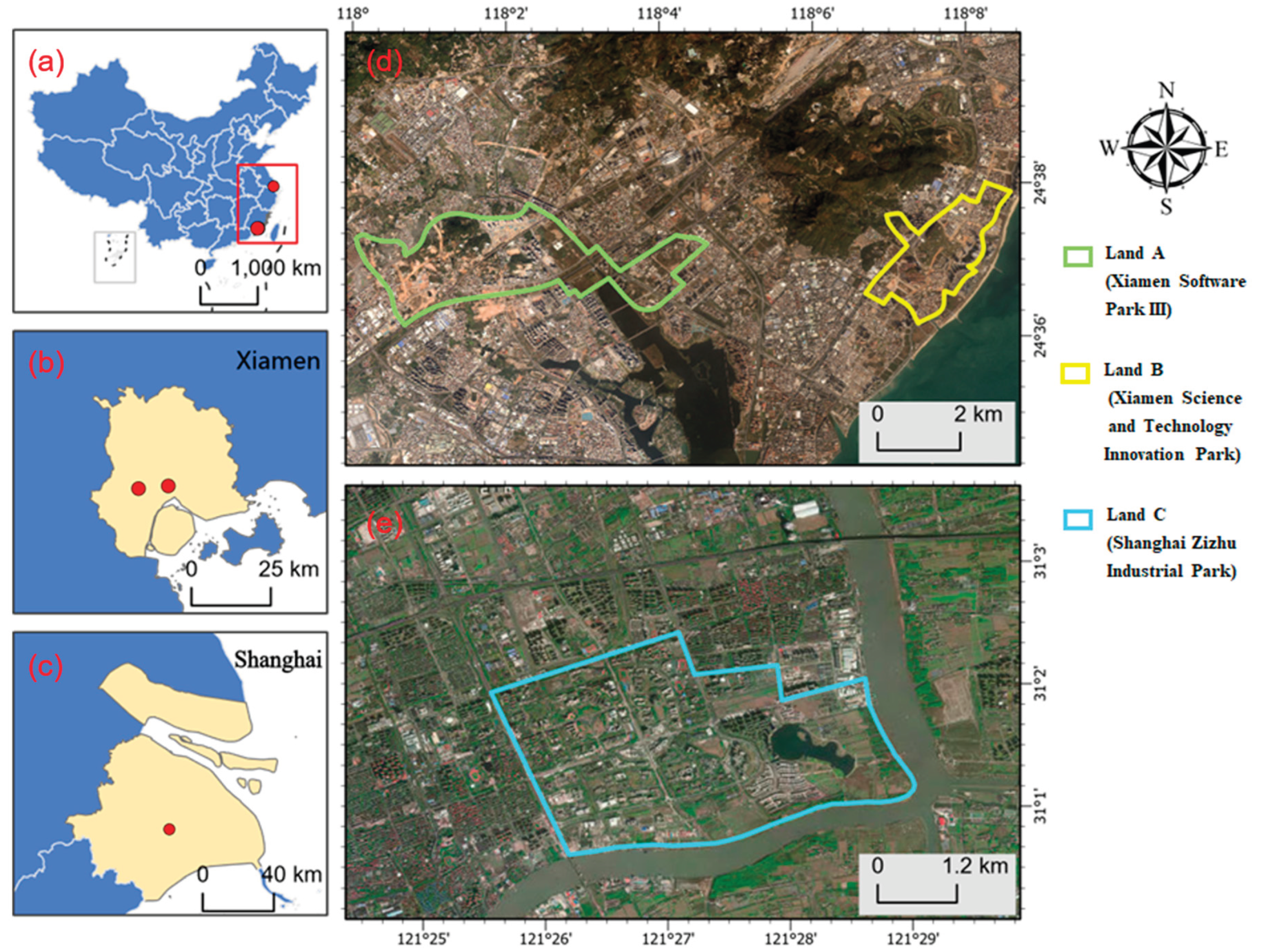
Figure 2.
The LSGP framework.
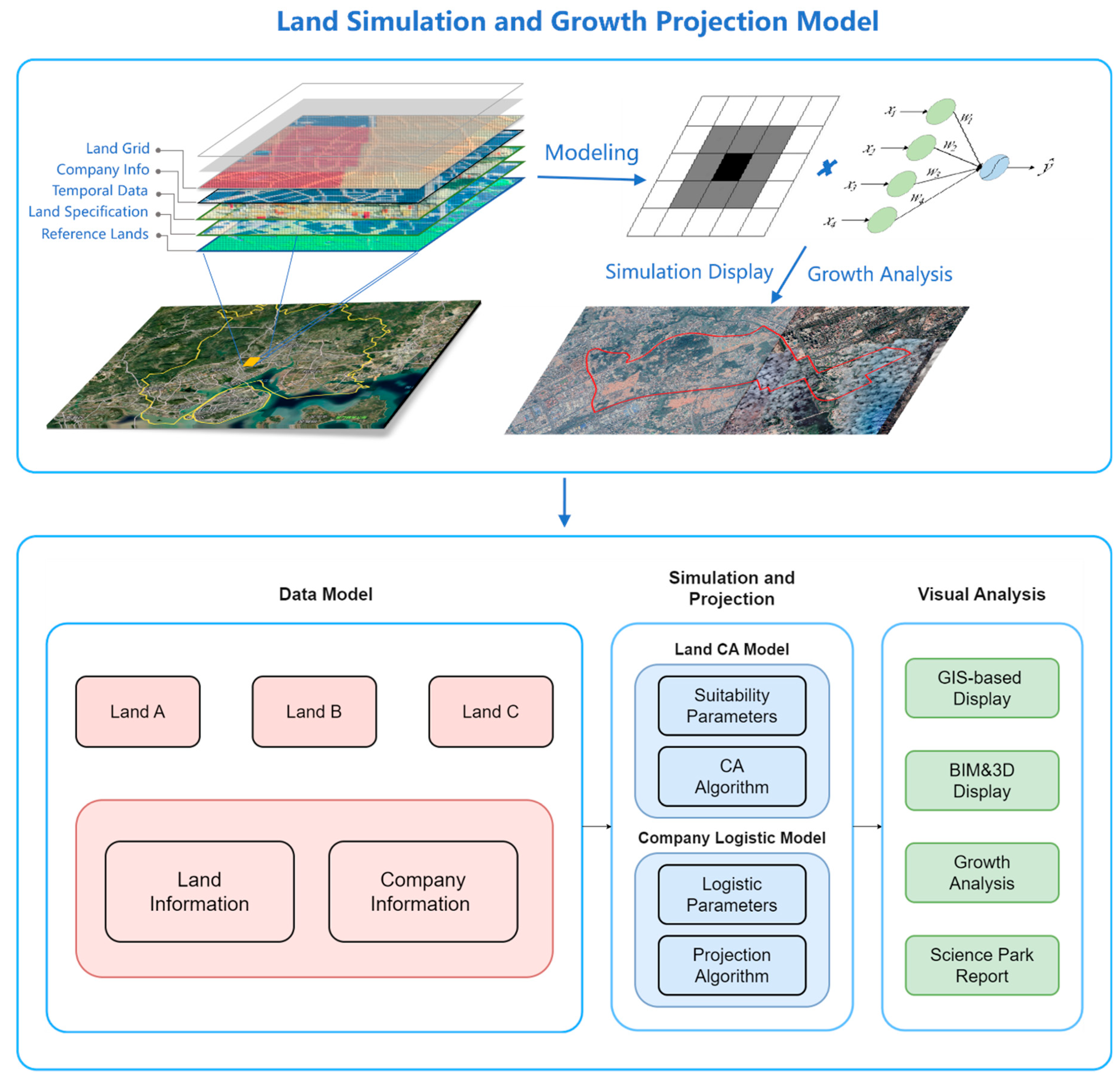
Figure 3.
Proposed method diagram for land use simulation and company growth projections.
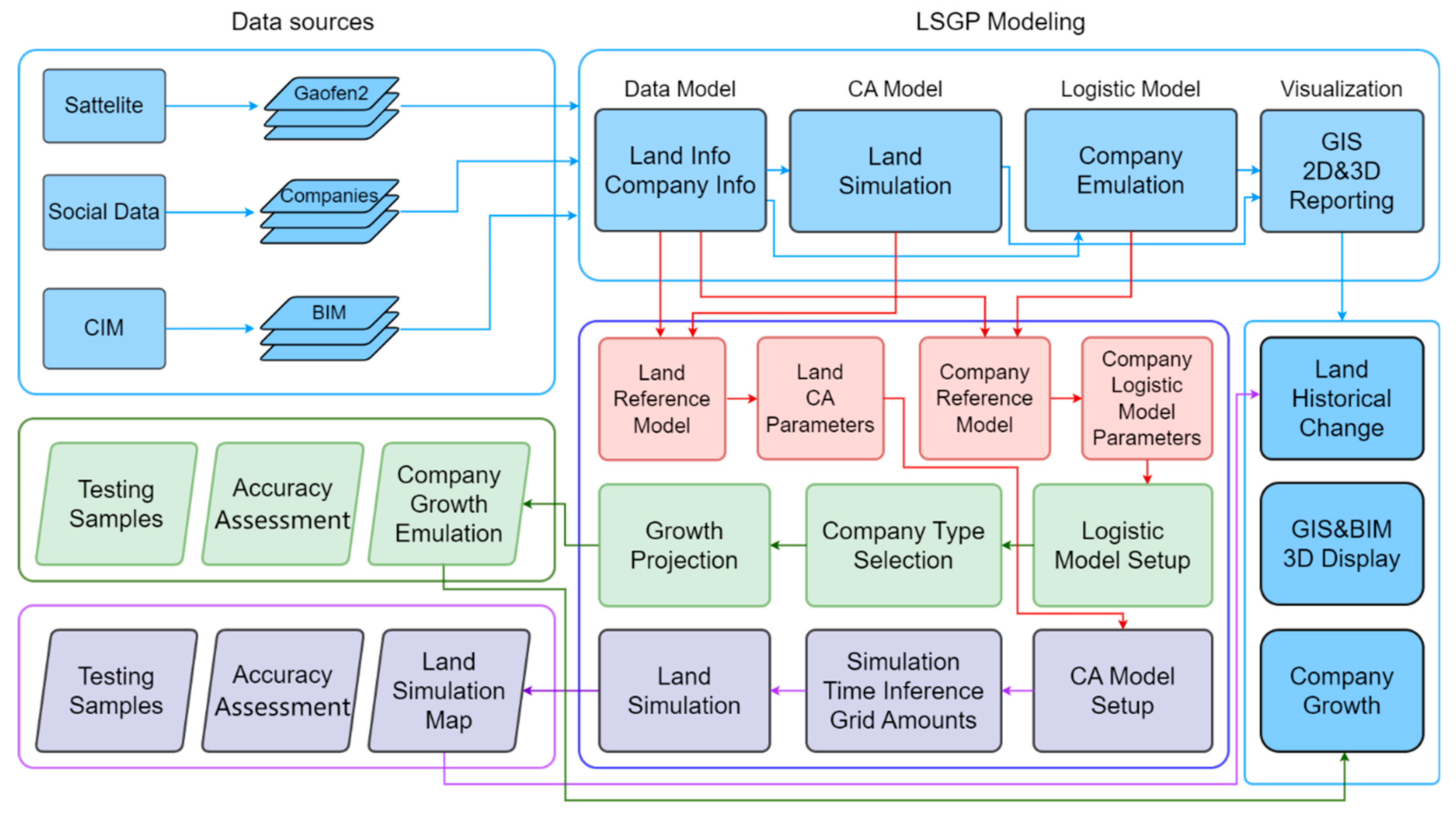
Figure 4.
Land development classification label of Land A.
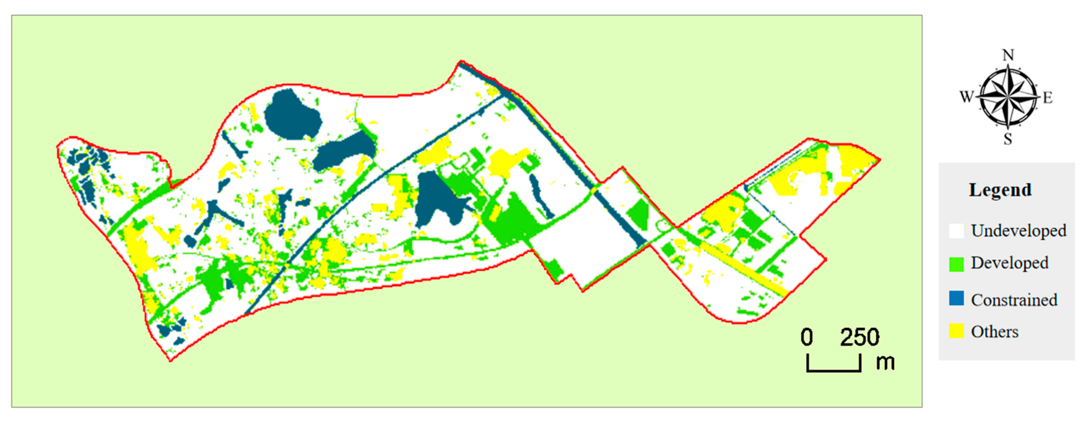
Figure 5.
Land A’s land development simulation result based on LR model and CA algorithm (in 2017).
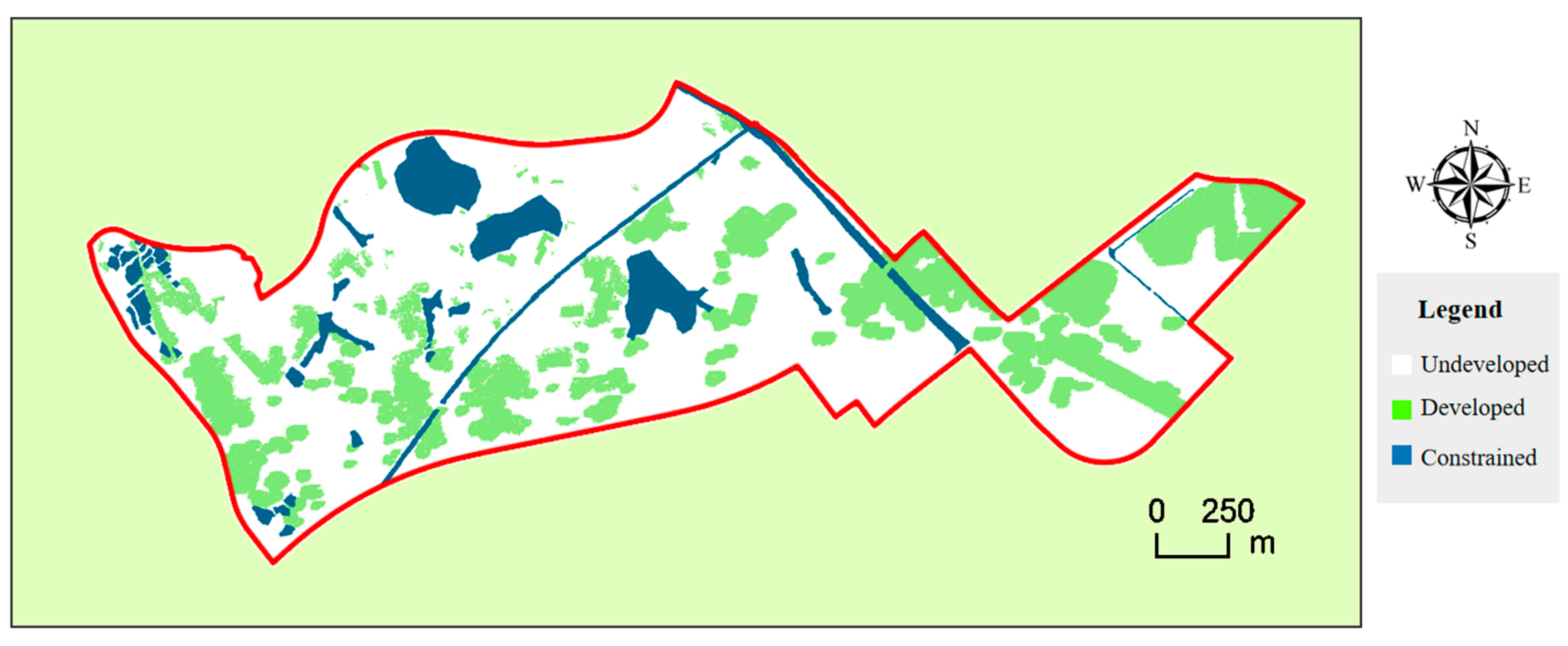
Figure 6.
Land A’s performance of land development simulation result based on LR model and CA algorithm: (a) OA changes and (b) FOM changes.
Figure 6.
Land A’s performance of land development simulation result based on LR model and CA algorithm: (a) OA changes and (b) FOM changes.
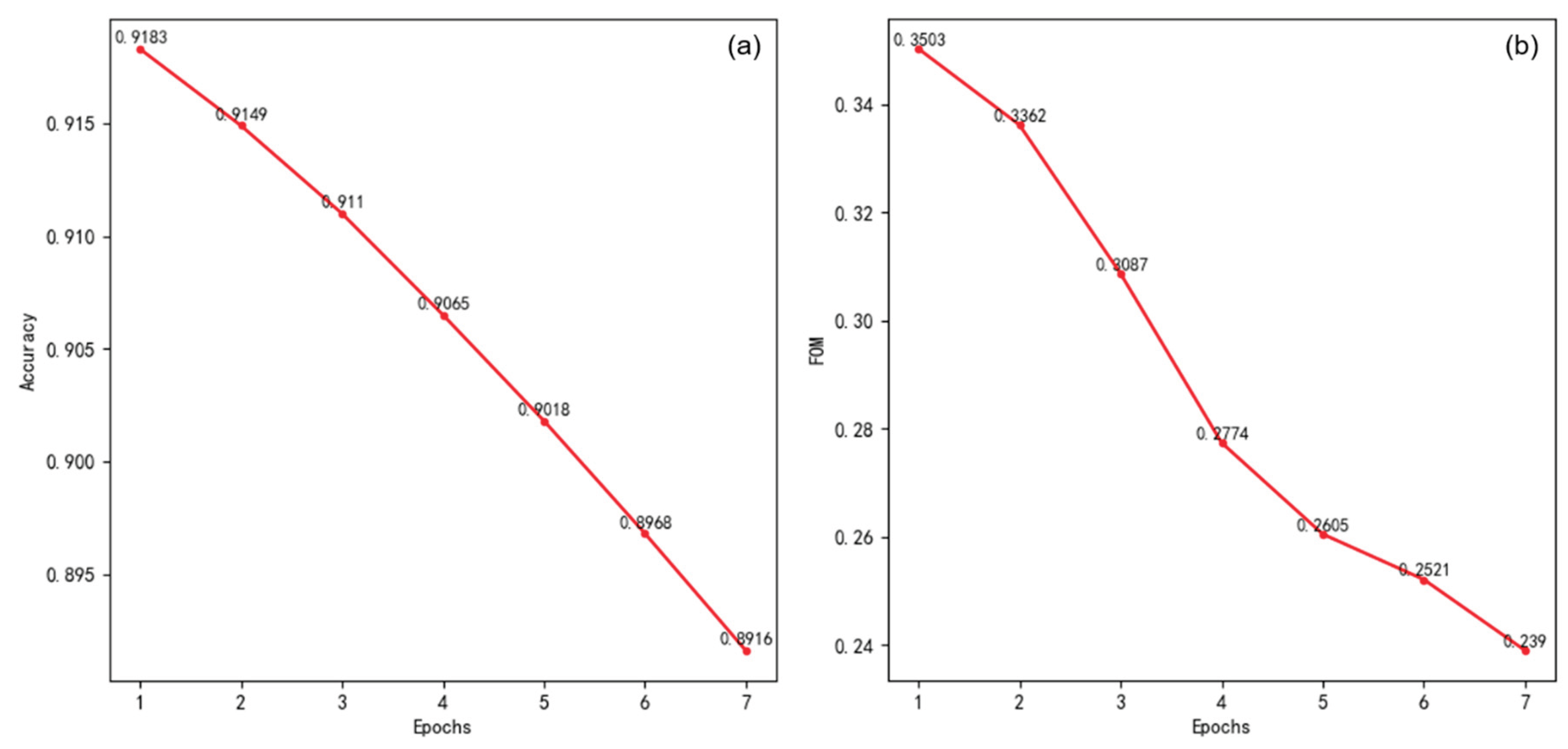
Figure 7.
The land development simulation result for Land A based on LR model transfer of Land B (in 2017).
Figure 7.
The land development simulation result for Land A based on LR model transfer of Land B (in 2017).
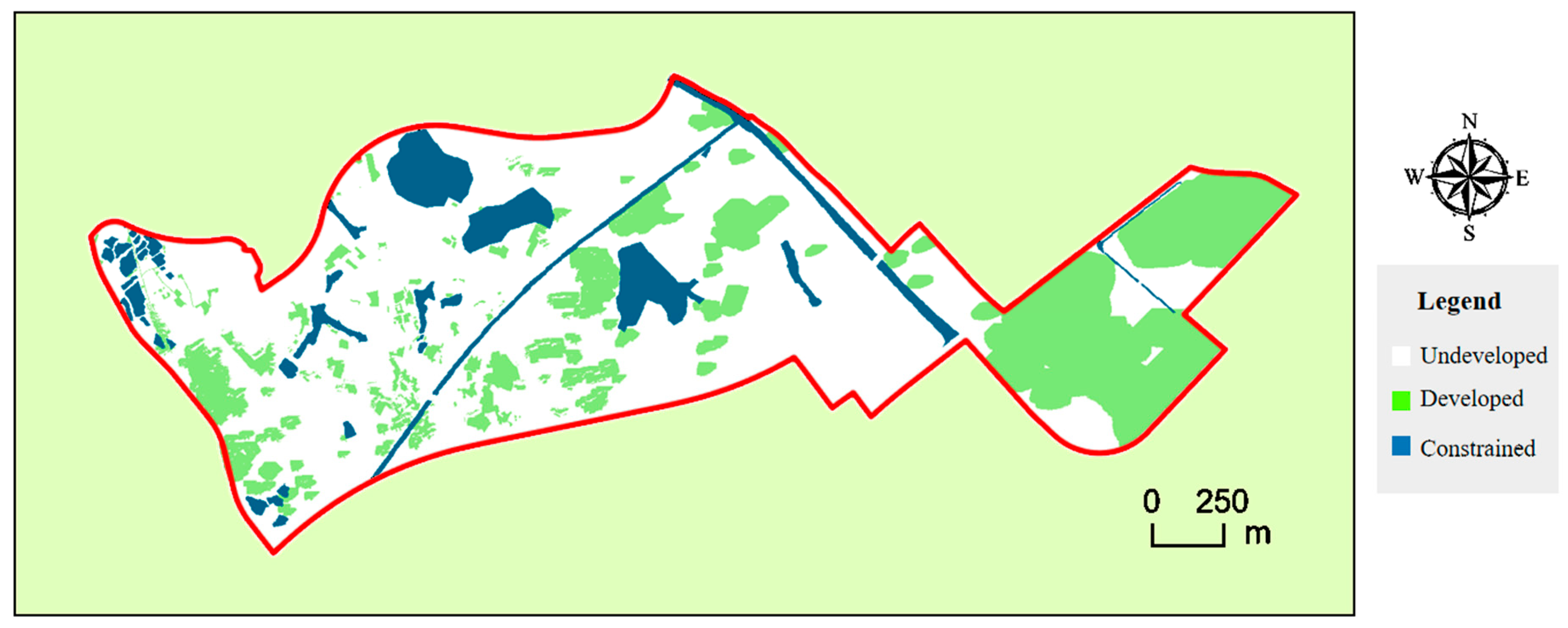
Figure 8.
The land development simulation result performance for Land A based on LR model transfer of Land B: (a) OA changes and (b) FOM changes.
Figure 8.
The land development simulation result performance for Land A based on LR model transfer of Land B: (a) OA changes and (b) FOM changes.
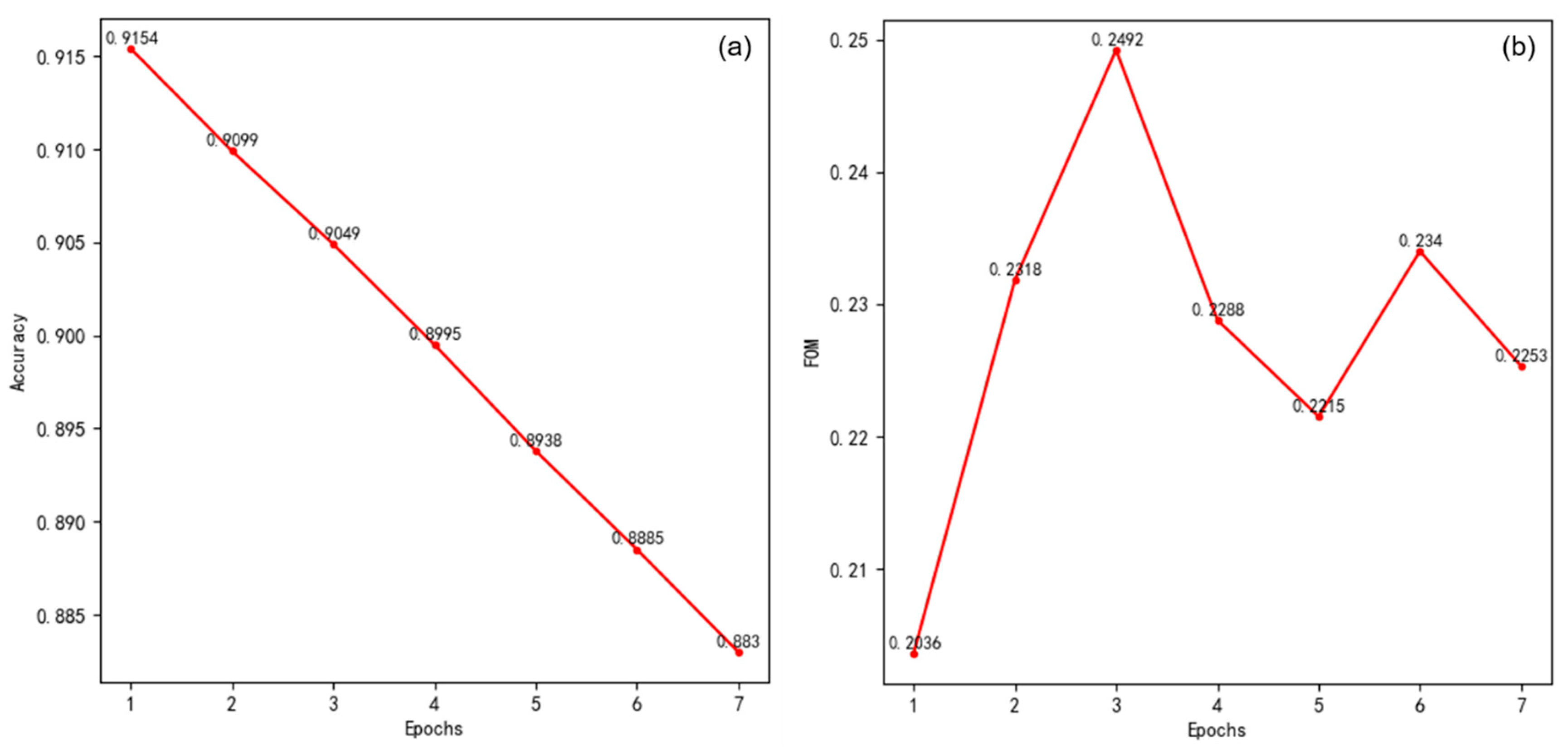
Figure 9.
The land development simulation result for Land A based on LR model transfer of Land C (in 2017).
Figure 9.
The land development simulation result for Land A based on LR model transfer of Land C (in 2017).
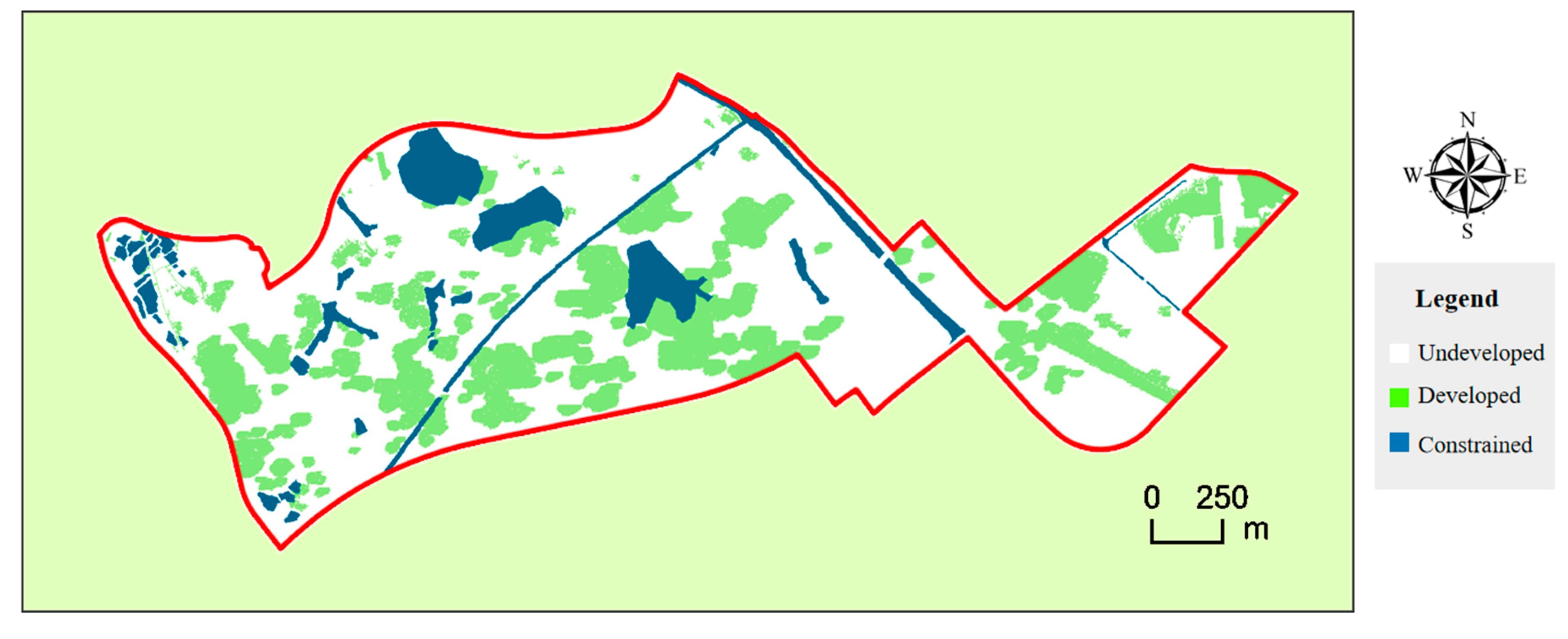
Figure 10.
The performance of land development simulation result for Land A based on LR model transfer of Land C: (a) OA changes and (b) FOM changes.
Figure 10.
The performance of land development simulation result for Land A based on LR model transfer of Land C: (a) OA changes and (b) FOM changes.
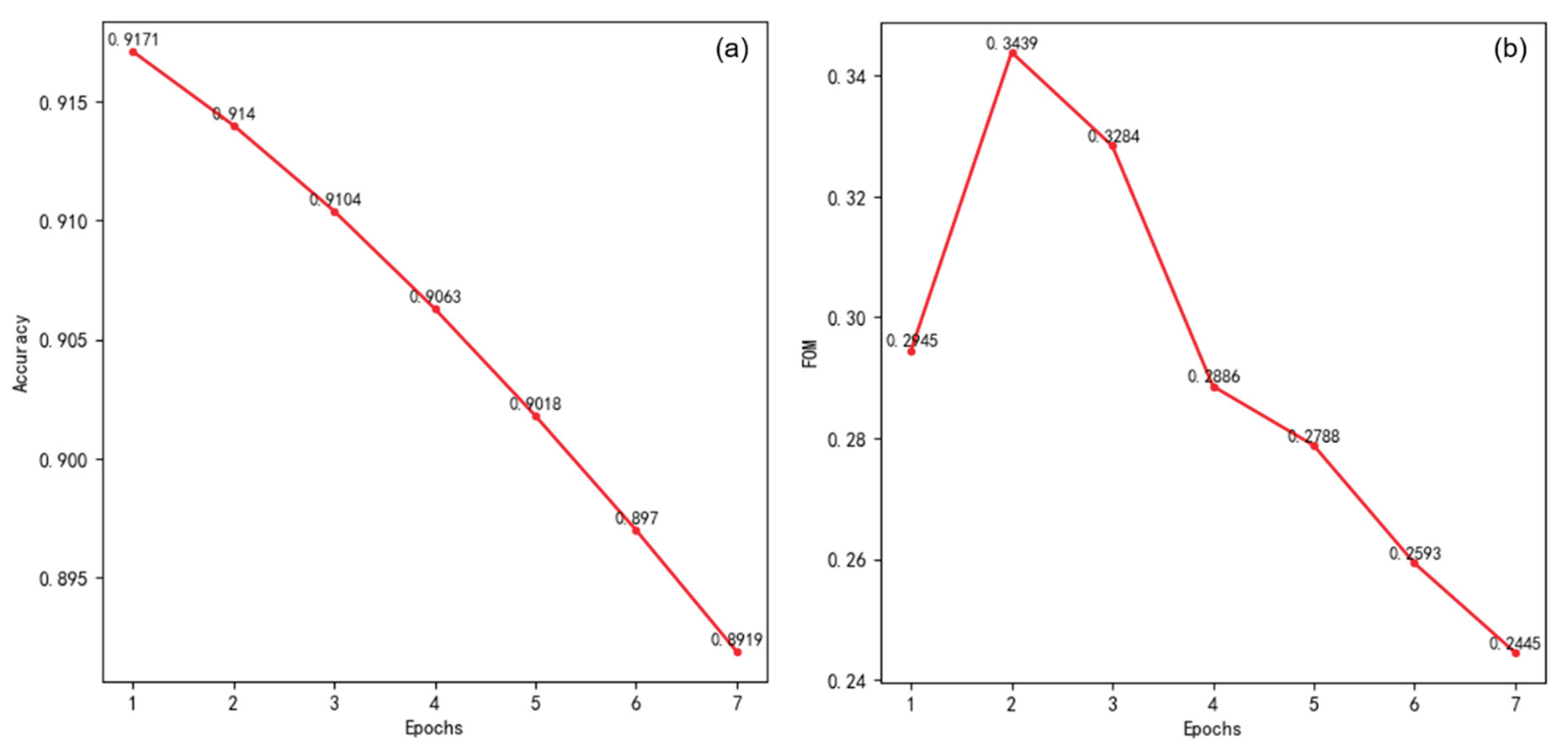
Figure 11.
The future land development simulation result for Land A (in 2035).
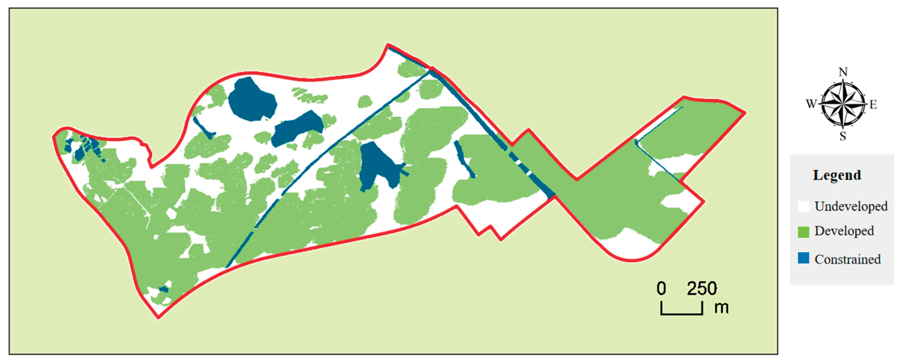
Figure 12.
The statistical and emulation results of company growth for Land A: (a) Statistical result; and (b) Emulation result.
Figure 12.
The statistical and emulation results of company growth for Land A: (a) Statistical result; and (b) Emulation result.
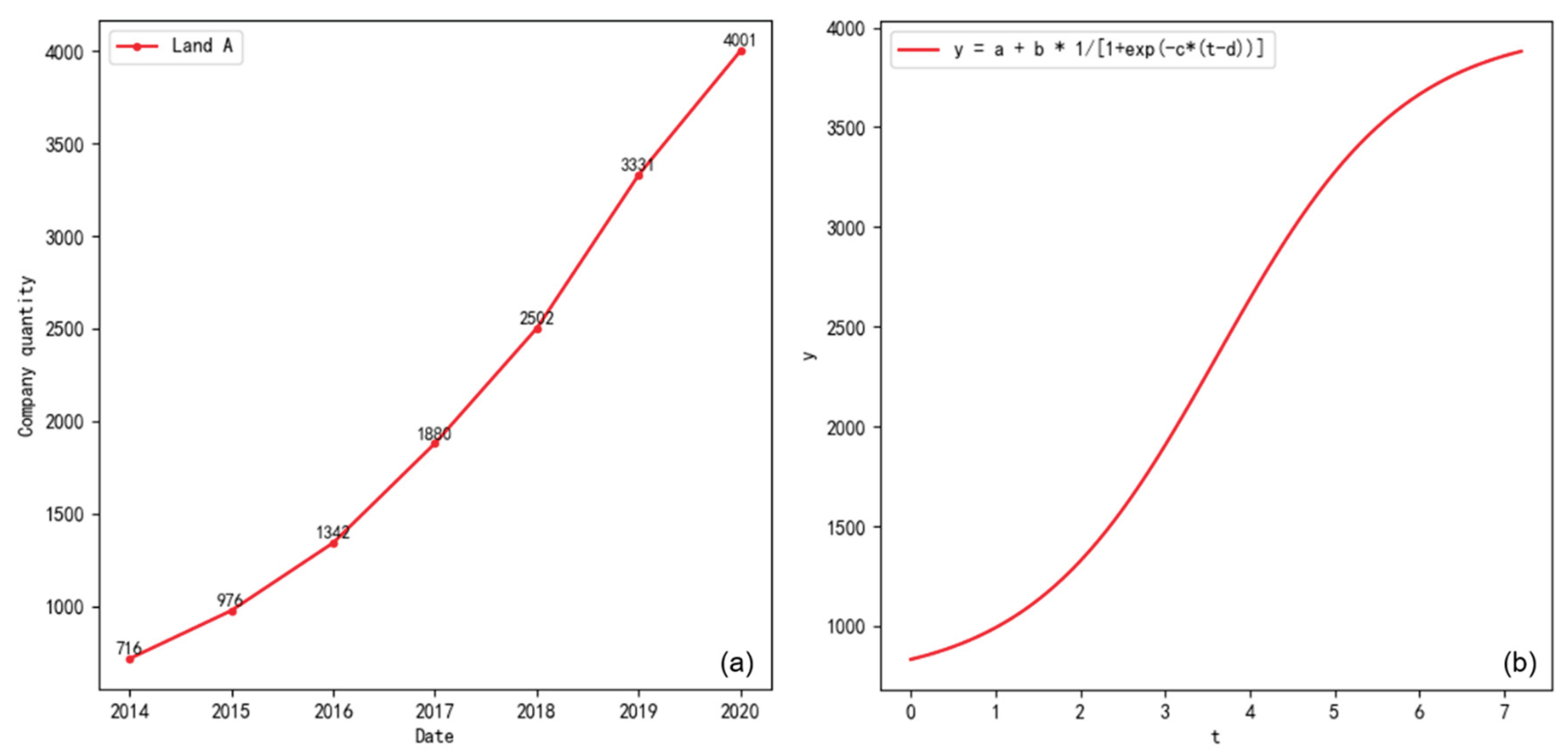
Figure 13.
The company growth emulation results in different industries for Land A: (a) Emulation results; and (b) Normalization results of graph (a).
Figure 13.
The company growth emulation results in different industries for Land A: (a) Emulation results; and (b) Normalization results of graph (a).
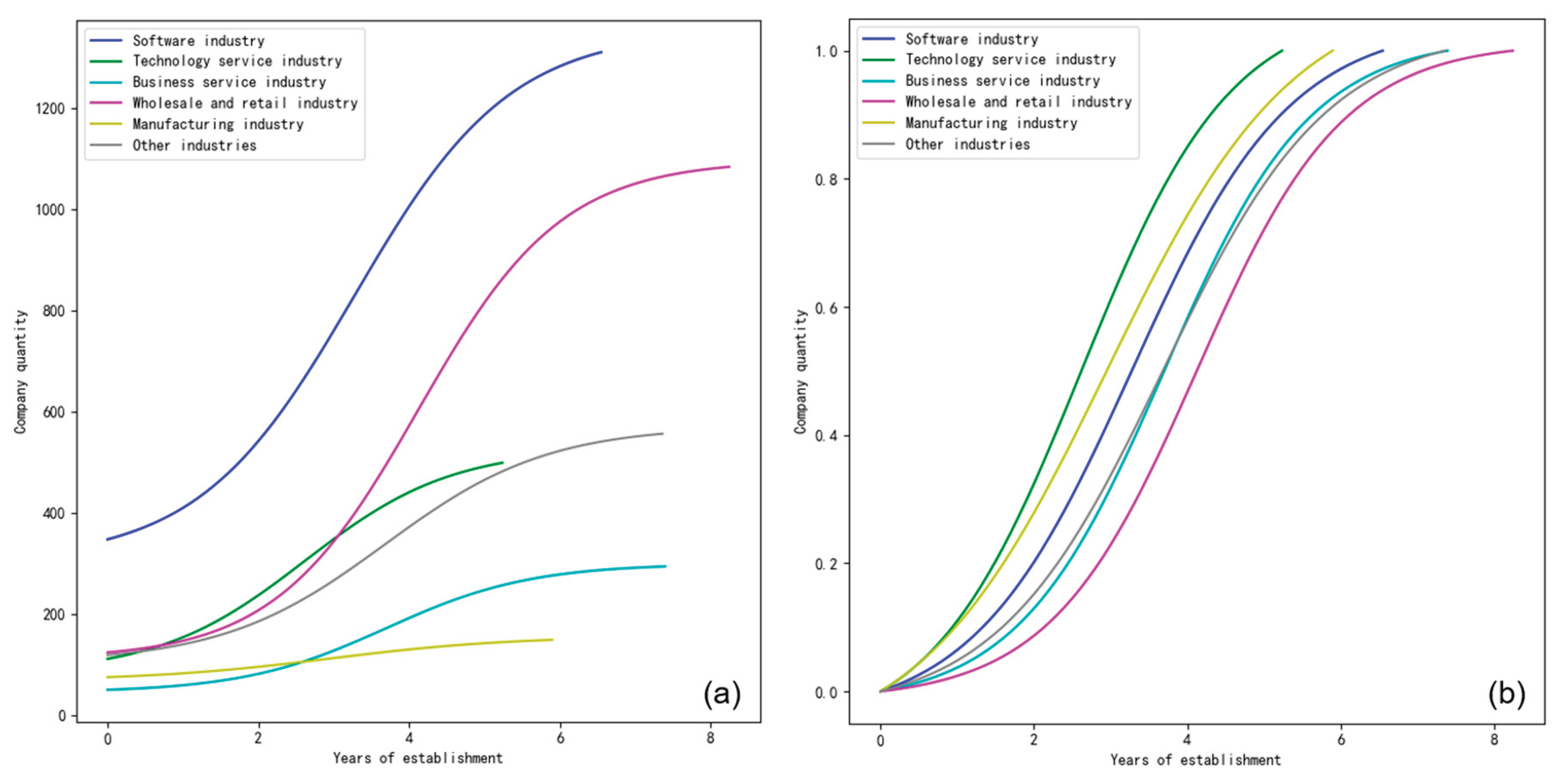
Figure 14.
The statistical and emulation results of company growth: (a) Land B; (b) Emulation result of graph (a); (c) Land C; and (d) Emulation result of graph (c).
Figure 14.
The statistical and emulation results of company growth: (a) Land B; (b) Emulation result of graph (a); (c) Land C; and (d) Emulation result of graph (c).
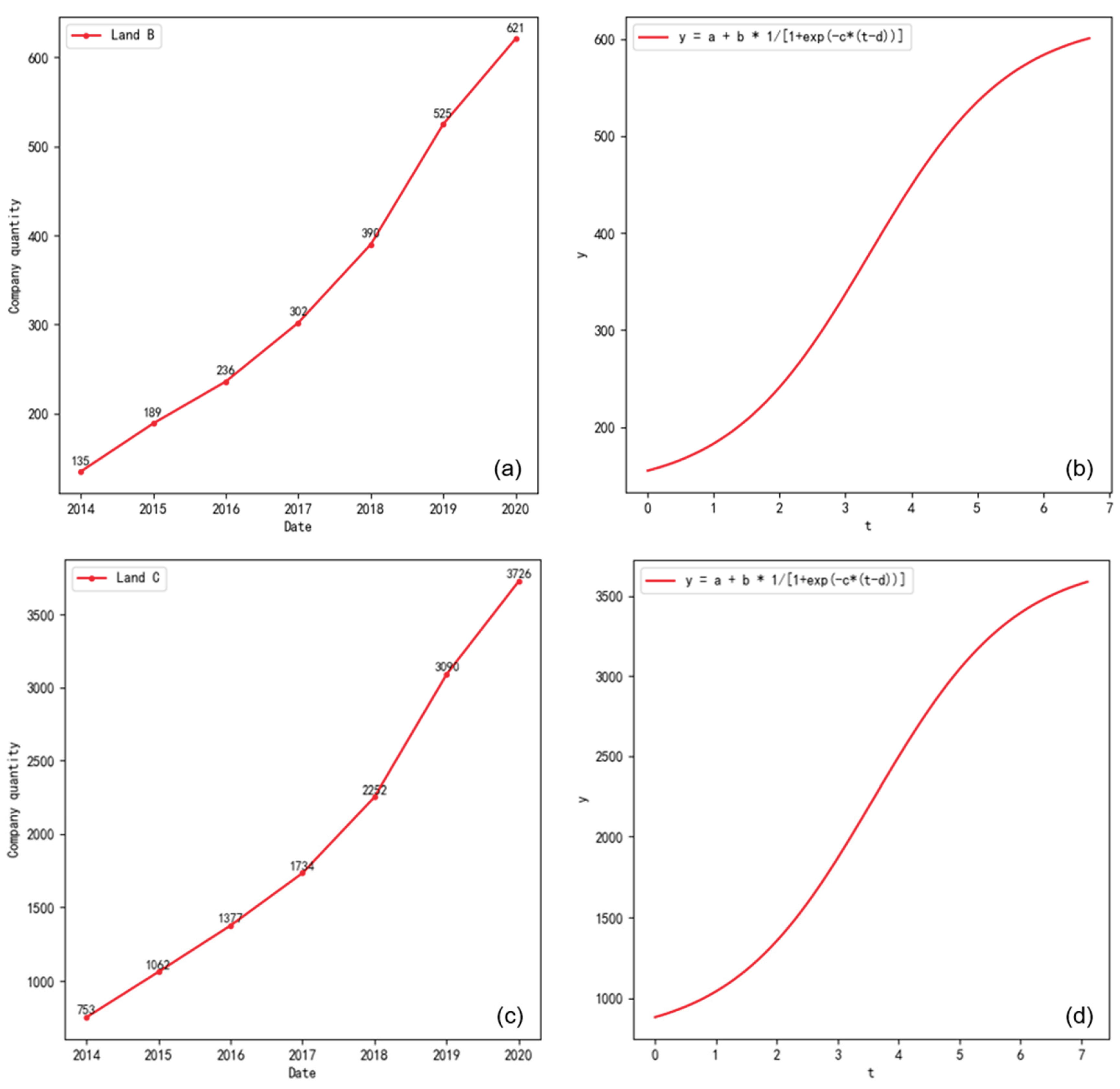
Figure 15.
The comparison of company growth emulation results for Land A based on LG model transfer in Land B and C.
Figure 15.
The comparison of company growth emulation results for Land A based on LG model transfer in Land B and C.
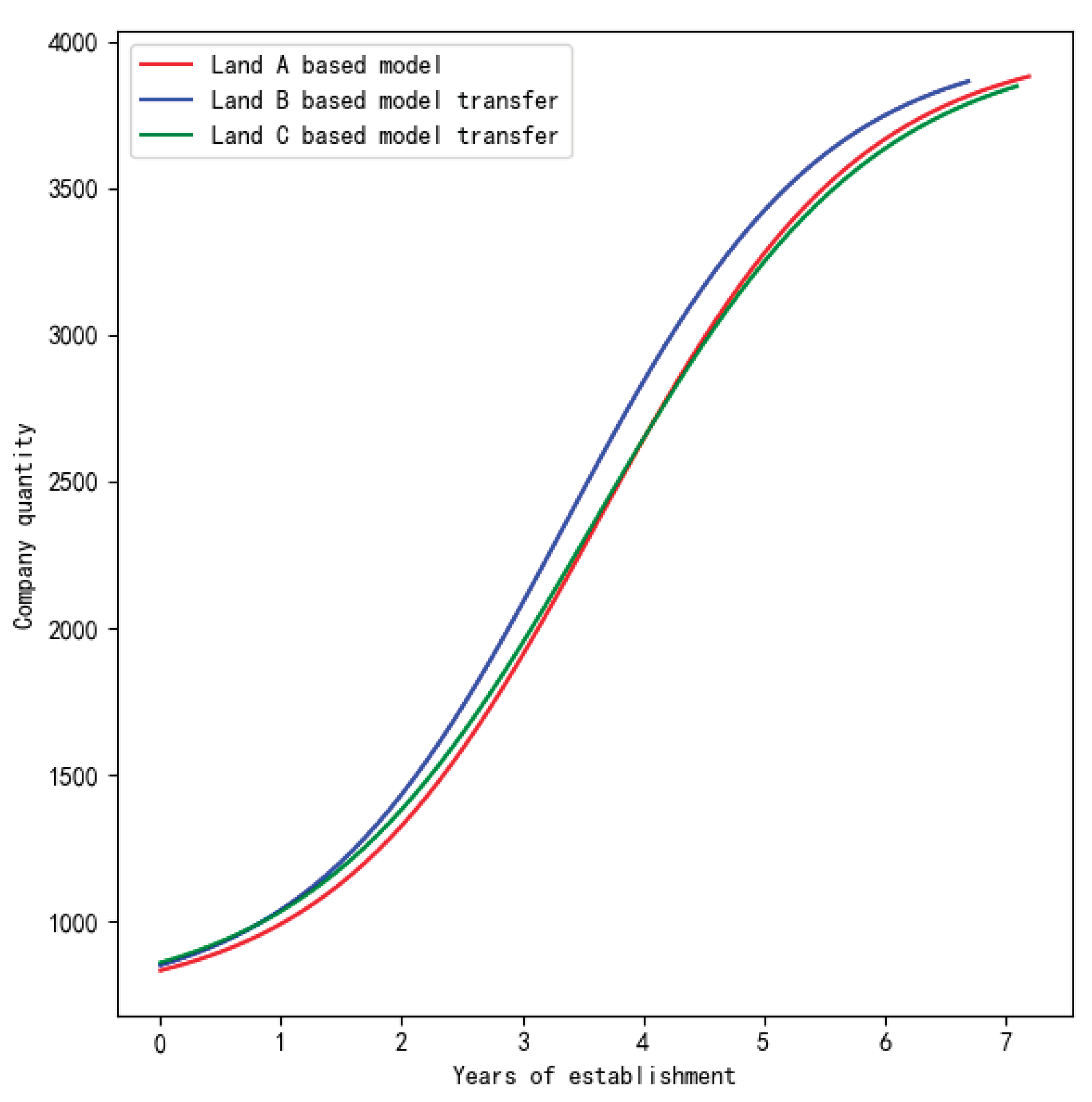
Figure 16.
The company growth emulation results: (a) Land A (2014-2028); (b) Land B (2014-2024); and (c) Land C (2014-2028).
Figure 16.
The company growth emulation results: (a) Land A (2014-2028); (b) Land B (2014-2024); and (c) Land C (2014-2028).
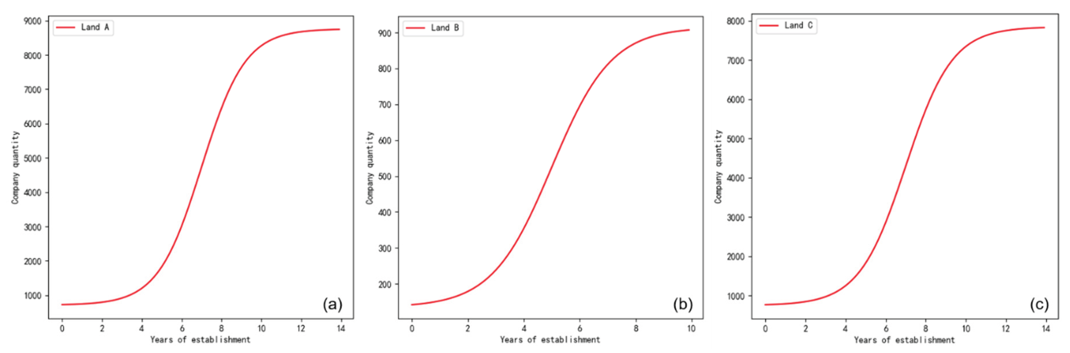
Figure 17.
The relationship between land development change and company growth: (a) Land A; (b) Land B; and (c) Land C.
Figure 17.
The relationship between land development change and company growth: (a) Land A; (b) Land B; and (c) Land C.
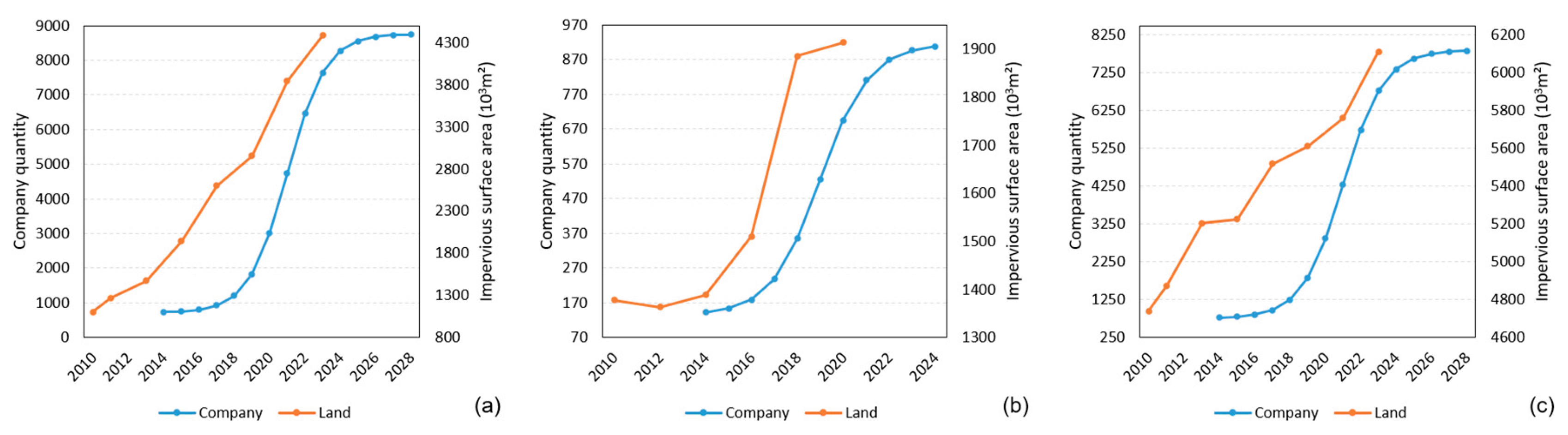

Table 1.
The features used to compute land development probability.
| Feature | Meaning |
| Main highway Main road Relief road Bridge in island Bridge out island Metro Market DEM Slope |
The distance feature from each pixel to the urban main road. The distance feature from each pixel to the main road in the park. The distance feature from each pixel to the relief road in the park. The distance feature from each pixel to the entrance of the bridge (located inside the Xiamen Island). The distance feature from each pixel to the entrance of the bridge (located outside the Xiamen Island). The distance feature from each pixel to nearby subway stations. The distance feature from each pixel to nearby market centers. The digital elevation model feature of each pixel. The slope feature of each pixel. |
Table 2.
The land development simulation results for Land A are compared based on different LR models.
Table 2.
The land development simulation results for Land A are compared based on different LR models.
| Model | OA | FOM |
| Land A based LR model | 0.9059 | 0.2892 |
| Land B based LR model | 0.8993 | 0.2277 |
| Land C based LR model | 0.9055 | 0.2911 |
Table 3.
The Parameters of LG Model for Different Industries in Land A.
| Industry | a | b | c | d |
| software industry | 305 | 1047 | 0.9668 | 3.2743 |
| technology service industry | 83 | 444 | 1.0256 | 2.6182 |
| business service industry | 45 | 254 | 1.0477 | 3.6975 |
| wholesale and retail industry | 111 | 985 | 1.0476 | 4.1226 |
| manufacturing industry | 68 | 88 | 0.8193 | 2.9479 |
| other industries | 104 | 467 | 0.9268 | 3.6798 |
Table 4.
LG Model Parameters for Different Lands.
| Land | a | b | c | d | MAE | R2 |
| A | 716 | 3285 | 0.9127 | 3.6203 | 36.2903 | 0.9983 |
| B | 135 | 486 | 0.9385 | 3.3600 | 7.5890 | 0.9969 |
| C | 753 | 2973 | 0.8599 | 3.5941 | 34.7067 | 0.9981 |
Disclaimer/Publisher’s Note: The statements, opinions and data contained in all publications are solely those of the individual author(s) and contributor(s) and not of MDPI and/or the editor(s). MDPI and/or the editor(s) disclaim responsibility for any injury to people or property resulting from any ideas, methods, instructions or products referred to in the content. |
© 2026 by the authors. Licensee MDPI, Basel, Switzerland. This article is an open access article distributed under the terms and conditions of the Creative Commons Attribution (CC BY) license (http://creativecommons.org/licenses/by/4.0/).
Copyright: This open access article is published under a Creative Commons CC BY 4.0 license, which permit the free download, distribution, and reuse, provided that the author and preprint are cited in any reuse.