

Submitted:
28 September 2026
Posted:
29 September 2026
You are already at the latest version
Abstract
A fixed-time stabilizer for underactuated Euler–Lagrange systems was established in Part 1 of this study , which certified fixed-time reaching on the actuated manifold and supplied a separate certificate for the internal dynamics. This paper asks what that certificate costs and what it buys. We decompose the total settling time into the reaching time governed by the certificate and an internal transient governed by the plant, and show that the two obey different constraints: the settling bound depends on the reaching gains alone and tightens exactly in inverse proportion to their scale, whereas the unactuated coordinate obeys a rate limit fixed by the coupling authority and is untouched by those gains. We prove that this forces a strictly positive floor on total settling time as the gains grow without bound, and we measure that floor to be far more binding in practice than the proof alone guarantees. On the translational oscillator with rotational actuator, scaling the reaching gains over a range of 13.3 tightens the analytical bound by a factor of 13.3 while the full-state settling time improves by 6.0% and the control energy rises by 53%. The floor is not an artifact of actuator saturation: with the actuation limit raised a hundredfold the same gain range still moves settling by only 11.4%. It is not an artifact of the plant either, since the cart-pole shows the separation more sharply, nor of the reaching-law gain family specifically, since settling varies by only 7.0% across a 49-design two-dimensional sweep over which the bound varies by a factor of 53.3. The floor is likewise unchanged at 1% and 5% settling tolerances, across a sixteenfold range of parametric mismatch including its sign, and under bounded disturbances, which the certified channel absorbs completely while the internal channel does not. A search over all eight controller parameters, a sampled-data implementation with measurement noise and torque quantization, three further cost metrics, and a fourfold finer sweep leave the result and the parity finding intact, and show that the designs that buy a tight certificate are also the ones that chatter and amplify noise. The bound itself is valid throughout, honoured by every design with margins between 62% and 95% once the event it governs is identified correctly. A matched-performance protocol puts the fixed-time law and its linear counterpart at energy parity, with ratios between 0.934 and 1.128. By contrast, increasing the coupling authority eightfold makes the response 7.4 times faster while reducing the energy integral by a factor of 14.6. The resulting design rule is to select gains against the guarantee that must be certified and to treat achievable response speed as a question about coupling authority rather than about feedback gain.
Keywords:
fixed-time stability
; gain selection
; underactuated systems
; Euler–Lagrange systems
; settling-time decomposition
; sliding-mode control
; internal dynamics
MSC: 93D40; 93C40; 70Q05
1. Introduction
Fixed-time stability strengthens the classical finite-time notion by requiring that the settling time admit a bound that holds uniformly over initial conditions [2,3]. For a designer this is an attractive guarantee: a single constant, computable from the gains before the system is switched on, certifies that the state will have converged by a stated instant regardless of where the trajectory began. The property is now available for a wide class of designs, from nonsingular fixed-time sliding-mode laws [4,5] to adaptive practical fixed-time schemes [6,7].
Such a design was established for underactuated Euler–Lagrange systems in Part 1 of this study [1], which proved fixed-time reaching on the actuated manifold and certified the internal dynamics that underactuation leaves unactuated. This paper takes that design as given and asks the question it does not: what a fixed-time guarantee costs and, above all, what it buys. The two are often conflated: a tighter settling bound is read as a faster controller, and the extra control effort spent to obtain it is justified by the speed it is presumed to deliver. In an underactuated mechanical system this reading fails, because the bound and the observable response are governed by different constraints.
The reason is structural. In the design of [1], partial feedback linearization splits the state into an actuated manifold, over which the feedback has full authority and on which fixed-time reaching is proved, and an internal coordinate reachable only through a bounded coupling term. The settling bound depends on the reaching gains alone. The internal coordinate, by contrast, obeys a rate limit set by the coupling authority, and no increase in an actuated-channel gain affects that limit. Certificate tightness is therefore purchasable without limit, while response speed is floored by the mechanics.
The consequence is quantitative and large: on the TORA benchmark, scaling the reaching gains over a range of tightens the analytical bound by a factor of and accelerates measured reach-and-hold on the actuated manifold by a factor of , while full-state settling time improves by , at a cost of more control energy. The gains buy a much better certificate and little response.
This paper makes three contributions. First, an analytical decomposition separates the part of the settling time controlled by the reaching gains from the part floored by the internal dynamics, and predicts a crossover past which further gain increases purchase certificate tightness only (Section 4). Second, a matched-performance comparison protocol: two controller families are compared at equal closed-loop performance rather than at equal gain labels, which is the only comparison from which a cost conclusion follows (Section 4.7). Applied to the fixed-time law and its linear counterpart, the protocol shows the two at energy parity, so fixed-time convergence is not intrinsically expensive. Third, a gain-selection rule follows from the decomposition: choose the gains against the guarantee that must be certified, and treat response speed as a question of coupling authority rather than feedback gain (Section 5.6).
Section 2 reviews the fixed-time and underactuated-control literature and, in Section 2.7, sets out what Part 1 established and what this paper adds (Table 1). Section 3 states the plant, the antecedent design, and the two structural facts the argument uses, with notation collected in Table 3 and every parameter value in Table 2. Section 4 develops the decomposition, states it as Proposition 1, and gives the matched-performance comparison protocol (Section 4.7). Section 5 reports the numerical study (after a convergence check, Section 5.1) and derives the gain-selection rule (Section 5.6) with a worked example (Section 5.6.1). Section 6 tests the floor’s robustness and generality: whether it is an artifact of actuator saturation, which reaching event the analytical bound governs (Section 6.5), whether it survives a second benchmark, a second gain direction, and a family the certificate does not constrain (Section 6.6), and whether it is sensitive to the settling criterion, to parametric mismatch, or to bounded disturbance (Section 6.7), and whether it survives a search over all gains, a sampled-data implementation, other cost metrics, and a finer grid (Section 6.8). Section 7 states the scope and limitations, including a networked extension (Section 7.6) and practical deployment (Section 7.4), and Section 8 concludes.
2. Related Work
The mechanism studied here, an unactuated internal coordinate that limits response independently of the controller applied to the actuated channel, is a special case of a non-minimum-phase or zero-dynamics obstruction, and the idea is classical rather than recent. Spong’s partial feedback linearization [8], used throughout this paper and its antecedent to separate the actuated and internal coordinates, and Olfati-Saber’s treatment of the cart-pole and rotating-pendulum benchmarks [9] establish the structural fact that an internal coordinate’s dynamics are not directly assignable by the actuated-channel controller; Theorem 1 is a fixed-time-specific instance of that fact, not a discovery of it. The review below is restricted to work published from 2020 onward, since that is when two narrower questions were first addressed quantitatively: how conservative a fixed-time settling estimate is relative to what is realized (the subsection on conservatism below), and what a fixed-time guarantee costs to obtain (the subsection on saturation and cost below). These are the questions this paper’s results extend, and the 2020 cutoff marks where that literature begins; it does not imply that nothing relevant to the paper predates it. The same obstruction is met in recent underactuated designs that must accommodate, rather than assign, an internal coordinate: Kasmalkar et al. [10] treat it explicitly as zero-dynamics mitigation for a feedback-linearized underactuated blimp.
2.1. Fixed-Time Stability Theory
The settling bound (2) is Polyakov’s [2] estimate for written on the sliding variable, and the theory around that inequality has continued to develop. López-Ramírez et al. [11] extend fixed-time stability to an input-to-state form through both explicit and implicit Lyapunov functions, Haddad [12] connects fixed-time stability to uniform strong dissipativity for feedback interconnections, and the predefined-time line [13,14] constructs dynamics whose settling-time bound is itself a design parameter rather than a tuning outcome. On the sliding-mode side, Tian et al. [5] and Zhang et al. [15] give nonsingular terminal designs with fixed-time guarantees of the same two-exponent form as (1). Two implementation questions raised by fractional-power laws have also received recent treatment: consistent discretization, since explicit integration can destroy the convergence property the continuous-time theorem guarantees [16,17], and chattering, addressed by continuous or practical fixed-time variants [18,19]. Throughout this literature the settling bound is the object of the theorem, and the question studied here, what tightening it purchases in the response of the full state, is not asked.
2.2. Fixed-Time Control of Underactuated Mechanical Systems
Fixed-time and terminal sliding-mode designs for underactuated plants have matured rapidly, with underactuated marine vehicles the most active application class: Zhou et al. [20], An et al. [21], and Fan et al. [22] combine fixed-time reaching laws with neural approximators, disturbance observers, or extended state observers for surface vessels and underwater vehicles. Rsetam et al. [23] develop a practically robust fixed-time convergent sliding-mode law for underactuated aerial systems, and Rojsiraphisal et al. [24] combine fast terminal sliding control with a disturbance observer for underactuated robots. Fan et al. [25] give a hierarchical sliding-mode fixed-time stabilizer for the cart-pendulum, following their swing-up and fixed-time stabilization of the cart-double-pendulum [26]; Jin et al. [27] combine a linear-quadratic outer loop with fixed-time adaptive sliding mode on the same plant; and Wu et al. [28] pair a non-singular terminal sliding surface with an extended state observer for an underactuated vehicle. The TORA benchmark used here has itself received recent attention, with global [29] and continuous [30] sliding-mode stabilizers and a nonlinear optimal design [31] alongside the following: Pan et al. [32] propose a model-free output-feedback stabilizer, Feng et al. [33] a disturbance-observer-based fixed-time design, and Guo and Liu [34,35] adaptive command-filtered and second-order backstepping schemes. These works establish convergence and report closed-loop trajectories, each with its own gains and settling figures for the benchmark. A direct numeric comparison against those figures was attempted for this revision but could not be completed reliably from the published abstracts and metadata alone, because the plant parameters, saturation limits, and settling criteria differ across the four papers and are not always stated in a form comparable to Table 2. None of the four papers report, however, how the settling estimate behaves as the reaching gains vary within a single design; this is the internal, single-controller comparison made here, as opposed to a comparison across different controllers.
2.3. Adaptive Fixed-Time Control of Euler–Lagrange Systems
For uncertain Euler–Lagrange dynamics, Zhu et al. [6] give an adaptive neural law with practical fixed-time tracking, Dong et al. [36] obtain fixed-time synchronization of networked uncertain Euler–Lagrange agents, and Zhao et al. [37] and Gao et al. [38] construct non-singular fixed-time sliding-mode laws, the former with a neural approximator and the latter with an explicit singularity-free surface. Liu et al. [39] use an interval type-2 fuzzy neural network within a fixed-time backstepping design, and Cui et al. [40] address distributed fixed-time attitude control under prescribed performance with event-triggered communication. This body of work is uniformly concerned with widening the class of admissible uncertainty: gain selection is treated as a tuning detail, and the settling bound is reported as a guarantee rather than examined as a design variable with a price.
2.4. Conservatism of Settling-Time Estimates
That the fixed-time bound is conservative is known, and sharpening it is an active line: Lin et al. [41] tighten the settling-time estimate for the class (2) belongs to, and Chen [42] derives tighter bounds for fixed-time stable systems in general. The mechanism here differs from the conservatism studied in this literature, and the distinction merits precise statement. Seeber et al. [43] study a class of differentiators with a predefined convergence-time bound and show it can be tuned arbitrarily tight for the same quantity the differentiator estimates: their conservatism is a gap between a bound and the realized time of the coordinate the bound is written for, closable by tuning. Sobański et al. [44] report the analogous gap for predefined-time vector-field-orientation control of mobile robots, again for the directly-actuated quantity. Xu et al. [45] estimate the energy cost of fixed-time synchronization for coupled networks, pricing the guarantee for the same synchronized state the bound describes. In each case, tightening the bound and improving the realized response are the same act, even if imperfectly matched by current tuning. This paper’s finding differs in kind, not degree: the bound (2) tightens exactly by construction ((5) is an algebraic identity, not a tuned approximation), so no residual conservatism gap remains for tuning to close, yet the response still does not follow, because the bound is written for one coordinate (the actuated sliding variable) while the observable settling time is limited by a different coordinate the bound was never written for. No amount of tuning the reaching gains closes this gap, because it is not a conservatism gap on the same quantity; it is a statement about two different quantities that share a common name, “settling time.” This is why Section 6.5 insists on distinguishing first-arrival from reach-and-hold: the conservatism literature above studies the analogue of the former, and this paper’s floor is a property of the latter.
2.5. Saturation and the Validity of the Bound
Several recent designs incorporate input saturation into fixed-time schemes. Fu et al. [46] handle actuator saturation in fixed-time formation control of marine vehicles; Fang et al. [47] treat saturated MIMO systems with fault tolerance, Van et al. [48] handle input saturation in distributed fixed-time consensus for multiple underwater vehicles, and Lei et al. [49] address prescribed-performance tracking for ships under actuator constraints. These works establish stability under saturation. The complementary question, addressed in Section 6.1, is whether an observed performance floor is an artifact of the actuator limit or a property of the plant; we answer it by relaxing the limit rather than by modelling it.
2.6. Position of This Paper
Across this literature, reaching gains are chosen to make a bound small, and the resulting closed-loop response is reported at those gains. We fix the plant and the controller family and vary the gains systematically, separating what the gains control from what they do not. The contribution is therefore not a new stabilizer but a measurement, a comparison protocol, and a selection rule for designs of the kind cited above.
2.7. Building on Part I: Theoretical Foundations and Contributions of the Present Study
This paper and [1] form a two-part study of one design, and they answer two different questions about it. Part 1 asked whether a fixed-time certificate can be established at all when an Euler–Lagrange plant is underactuated and its parameters are uncertain in the matched channel. It answered by construction: partial feedback linearization, a recursive fixed-time backstepping law, and a -modified adaptation law, together with two proofs, a settling-time bound (2) on the actuated channel and an internal-dynamics certificate for the coordinate that underactuation leaves unactuated, which removes the minimum-phase assumption. This paper takes that design as given and asks what its certificate costs and what tightening it buys. That question is not raised in Part 1, and answering it needs machinery Part 1 has no use for: a one-parameter family of gains, sweeps over that family on two benchmarks, a protocol for comparing controller families at matched closed-loop performance rather than at equal gain labels, and falsification tests for the mechanism proposed to explain the result. Table 1 sets the two papers side by side.
One inequality from Part 1’s internal-dynamics certificate is used in the argument below. Theorem 1 restates it with a self-contained proof, so that step does not depend on [1]; the original numbering is noted so the two papers can be read together. Everything else is new: the decomposition of settling time into a certificate-governed phase and a plant-governed phase (Section 4), Proposition 1 and its proof, the comparison protocol (Section 4.7), the sweeps and the knee they locate (Section 5), the eleven structural controls (Section 6), and the gain-selection rule (Section 5.6).
3. Problem Setup and the Antecedent Design
We consider the class of underactuated Euler–Lagrange systems treated in [1]. The generalized coordinates are , with actuated component and unactuated component ; the dynamics are , where M is uniformly positive definite and the unactuated inertia block is invertible on the operating domain. The uncertainty is matched and linearly parameterized: after partial feedback linearization [8], the actuated dynamics become , where y is the partially linearized output, v is the virtual control, Y is a known measurable regressor, and is an unknown constant vector.
The controller of [1] regulates the actuated error through the sliding variable , where , and drives s to zero with the bi-limit reaching law
with and , together with the -modified adaptation , whose leakage keeps bounded without persistency of excitation. The composite Lyapunov function yields the fixed-time differential inequality on the actuated channel, from which the settling bound follows.
Two structural facts drive everything below. The first is the form of the bound. Written directly on the sliding variable, the reaching time of (1) satisfies
which depends on the reaching gains and the fractional exponents alone. No property of the plant, and in particular no property of the unactuated subsystem, appears in (2).
The second is the rate limit on the internal coordinate. Writing for the internal coordinate and for its energy, Theorem 3(iii) of [1] establishes
where bounds the coupling authority of the actuated coordinate over the unactuated one.
Theorem 1
(Internal rate limit). Along any closed-loop trajectory the internal energy satisfies (3). Consequently the settling time of the internal coordinate is amplitude-dependent and is bounded below by a quantity determined by ε, independently of the reaching gains.
Proof.
The internal coordinate obeys with bounded forcing (the coupling from the actuated coordinate, saturated at ). With ,
so and, using wherever ,
which is (3). Integrating gives , so internal energy cannot be extracted faster than a rate fixed by , however the actuated channel is driven; the time for to settle therefore scales with its initial amplitude and is not fixed-time. This argument is self-contained and independent of the sign or stability of the plant’s open-loop zero dynamics. The fuller certificate, comprising this result together with separately established boundedness (ISS) and asymptotic convergence of , is Theorem 3 of [1], from which the labelling above is retained for continuity with that manuscript. □
The internal coordinate cannot be driven toward the origin faster than a rate fixed by ; its settling time is amplitude dependent and is not fixed time. We refer to (3) as Theorem 1.
The numerical study uses the TORA benchmark as instantiated in [1]: coupling coefficient , internal coordinate , and a saturated virtual target with enforcing . The plant has one internal coordinate; the multi-coordinate case is outside the present scope (Section 7). Table 2 lists every controller parameter and physical constant used in the study for both benchmarks, so the numerical results are reproducible from this manuscript alone.

Table 2.
Controller gains and physical parameters used throughout. TORA gains are those scaled by (or , Section 6.6.4) in the sweeps; cart-pole gains are held fixed at the design values reported in Section 6.6.
Table 2.
Controller gains and physical parameters used throughout. TORA gains are those scaled by (or , Section 6.6.4) in the sweeps; cart-pole gains are held fixed at the design values reported in Section 6.6.
| quantity | symbol | value | benchmark |
|---|---|---|---|
| coupling authority | TORA | ||
| matched-uncertainty parameter | TORA | ||
| saturation ratio | TORA | ||
| tracking-error gains | TORA | ||
| tracking-error exponents | TORA | ||
| reaching-law gains (design, ) | TORA | ||
| reaching-law exponents | TORA | ||
| outer virtual-control gains | TORA | ||
| outer virtual-control gains | TORA | ||
| outer exponents | TORA | ||
| adaptation gain, leakage | TORA | ||
| virtual-acceleration clip | 50 | TORA | |
| cart mass, pendulum mass | cart-pole | ||
| pendulum length, gravity | cart-pole | ||
| cart-loop gains | cart-pole | ||
| lean and tilt limits | cart-pole | ||
| tracking-error gains | cart-pole | ||
| reaching-law gains (design, ) | cart-pole | ||
| reference time constant | cart-pole | ||
| adaptation gain, leakage | cart-pole | ||
| matched-uncertainty parameter | cart-pole |
Table 3.
Nomenclature for the time and gain quantities: the four times are distinguished throughout, with two representing guarantees and two representing measurements.
Table 3.
Nomenclature for the time and gain quantities: the four times are distinguished throughout, with two representing guarantees and two representing measurements.
| Symbol | Name | Meaning |
|---|---|---|
| certificate, bound | Analytical settling bound (2) on the sliding variable. A guarantee, computed from the gains before the run. | |
| first-arrival time | Measured time at which the sliding variable first enters the tolerance band; the quantity that (2) bounds. Distinct from the reach-and-hold time, the first instant after which it remains in the band (Section 6.5). | |
| internal transient | Time for the unactuated coordinate to converge after first arrival. Floored by through (3). | |
| full-state settling | Measured time for the whole state to enter and remain in the band. Equals by (4). | |
| reaching-gain scale | Multiplier applied to . | |
| reaching exponents | Fractional powers in (1), . | |
| coupling authority | Bound on the actuated coordinate’s influence over the unactuated one. A property of the mechanism, not of the controller. | |
| virtual-acceleration clip | Saturation limit in the implementation. |
4. What the Gains Control
This section separates the settling time into two parts and shows that the reaching gains act on one of them only.
4.1. Decomposition
Let denote the time for the full state to enter and remain in a neighbourhood of the origin, and let denote the first-arrival time to the actuated manifold: the first instant at which the sliding variable enters the tolerance band (Section 6.5 distinguishes this from the reach-and-hold time and shows only first-arrival is bounded by (2)). Write for whatever time remains after first arrival; since the phases are sequential in this sense,
This is an identity, true by definition of , not yet a statement about what controls . By (2), is bounded by , a function of the reaching gains. Whether is itself independent of the reaching gains is exactly the question Section 4.3 below addresses; the naive argument that it is, by appeal to Theorem 1 alone, does not survive a check against the data and is corrected there.
4.2. Scaling the Reaching Gains
Introduce a single family scale applied multiplicatively to the reaching gains, . Both terms of (2) are inversely proportional to their gain, so
The certificate therefore tightens exactly in proportion to , without saturation and without any dependence on the plant. The exponents and are unchanged by the scaling, so the bi-limit structure that produces fixed-time behaviour is preserved along the family.
A first pass runs as follows: the gains act on the sliding variable of the actuated channel and do not appear in (3), whose right-hand side is set by , a structural constant of the mechanism, so one might expect to be exactly unchanged by and for every . This intuition motivates the separation but is not quite right, for the reason given in Section 4.3 immediately below: inherits whatever is measured to be, and if is taken as the reach-and-hold time rather than first-arrival, computed this way is not constant. Proposition 1 replaces the intuition with a provable statement.
4.3. A Corrected Statement of What Is Actually Invariant
An earlier version of this argument claimed that the post-reaching internal transient is exactly independent of , and used for the reach-and-hold time to conclude for every . Neither claim survives a check against the data in Table 6 and Table 13: bounds first-arrival, not reach-and-hold (Section 6.5), and the reach-and-hold time itself varies by more than a factor of ten across the sweep, so computed by subtraction is not constant. The following replaces that argument with one that is actually provable, and is weaker in exactly the way the data requires: it establishes that a floor exists, not that it is achieved at every .
4.4. Statement of the Separation
Let denote the first-arrival time to the actuated manifold, the quantity that (2) provably bounds (Section 6.5), and let denote the internal coordinate and its rate. Write for the internal energy.
Proposition 1
(Certificate–response separation). Consider the closed loop of Section 3 with reaching gains scaled by , as above, subject to the rate limit (3) with coupling authority ε independent of κ. Then:
- the certificate satisfies exactly, so as ;
- as , and by continuity of the flow in κ, ;
- consequently, for any tolerance with , the time required for to first fall to η after satisfies
Since , item (iii) gives , while by item (i); the ratio is therefore unbounded as .
Proof.
Item (i) is (5). Item (ii): follows from (Section 6.5 establishes the bound for first-arrival specifically); the state at time converges to the state at by continuous dependence of solutions on the integration horizon, so . Item (iii): the rate limit (3) gives for , so cannot fall to before ; taking and using and gives the stated lim inf. □
This is deliberately weaker than the earlier statement. It proves that a strictly positive floor exists in the limit ; it does not claim is constant, or equal to the floor, at every finite , and it says nothing about measured by reach-and-hold rather than by the internal energy’s own decay. Table 4 reports the quantity the proof actually controls, , across the sweep: it is constant to within and converges to as grows, exactly as item (ii) predicts, and the induced floor s is a valid, if loose, lower bound on every in Table 6 (all of which exceed s). The much tighter empirical variation reported in Section 5 is a numerical finding, not a consequence proved by Proposition 1; the proposition establishes that a floor of this kind must exist, and Section 5 measures it to be far more binding in practice than the proof by itself guarantees.
4.5. The Knee: An Empirical Transition, Located by Bisection
Table 6 and Figure 1 show a sharp transition in the reach-and-hold time between and . Bisecting that interval to a tolerance of in locates the transition at : the reach-and-hold time falls from s at to s at . Below this value, increasing buys a roughly proportional reduction in reach-and-hold time; above it, the reach-and-hold time continues to fall but far more slowly, and by it has entered the regime reported in Section 5, where a -fold further increase in changes the full-state settling time by only . We call the knee of the design. Unlike the earlier draft of this argument, no claim is made that the knee marks a crossover between and a -invariant ; Section 4.3 retracts that specific mechanism. The knee is reported here as what it is: a measured feature of the reach-and-hold curve, worth knowing when choosing , and consistent with (but not proved by) the floor established in Proposition 1.
Past the knee, the guaranteed bound keeps tightening at the undiminished rate (5), because it is a statement about the actuated channel alone. The measured full-state response does not track it, for the reasons documented empirically in Section 5 and Section 6.6 across two benchmarks, a coupling-authority sweep, and a two-dimensional gain grid. Any control effort spent past the knee purchases certificate tightness and little else.
4.6. Weight of the Internal Phase
The decomposition matters only if is a substantial fraction of . Table 5 reports this measurement directly. At the design gains (), the reaching phase accounts for of the full-state settling time at , at , and at . The internal phase thus ranges from one fifth to just over one half of the total, with its share largest at small initial conditions.
The direction of that trend follows from (3). The internal transient is bounded below by a quantity that grows with the initial internal amplitude but is capped in rate by , whereas the actuated reaching time grows toward its initial-condition-independent ceiling . As increases, the reaching term approaches a constant while the internal term keeps growing, so the reaching share rises. At small , the reaching time is already well below its ceiling, and the internal phase dominates. In both regimes the internal phase is too large to neglect, which is what makes the floor established by Proposition 1 a practical constraint rather than an asymptotic curiosity, and why Section 6.1 and Section 6.5 repeat their controls at and rather than at alone.
4.7. The Matched-Performance Protocol
Comparing two controller families requires care about what is held fixed. The comparison usually reported holds the gain values fixed and substitutes one reaching law for another. That choice is not neutral. In (1) the coefficient multiplies with , whereas the linear counterpart used throughout this comparison is the same architecture with every fractional-power term replaced by a linear term carrying the same coefficient. At the reaching law,
and at the outer virtual control, in place of the fractional-power form of Table 2. The same multiplicative scale acts on in both families, so the two share every gain value and differ only in the exponents, all of which are set to one in the comparator. The simulation module shipped with this paper contains both controllers and reproduces every row of Table 6 exactly. The two reaching terms have different units and different magnitudes at every , so equal gain labels do not describe equally aggressive controllers, and an energy difference measured that way reports the tuning as much as the law.
The comparison from which a cost conclusion follows holds a closed-loop performance measure fixed and compares the cost of achieving it. We adopt the following protocol.
- Parameterize each family by one scale. Apply multiplicatively to as in Section 4. This traverses each family along a one-dimensional curve while preserving its structure.
- Sweep both families over the same grid. We use 13 points spaced logarithmically over , and record for each point the full-state settling time and the control energy.
- Select at a common performance level. Take the target settling time to be the worse of the two families’ best native settling times over their sweeps, that is, the slower family’s best achievable settling, so the target is attainable by construction for at least one point in each family. For each family, take the smallest energy attained by any sweep point that settles at least as fast as this target. This is a Pareto selection rather than an interpolation, so it does not assume energy is monotone in settling time, and Table 7 is reproducible from the two 13-point sweeps by this rule alone.
- Report the ratio of energies at matched settling. This is the quantity that answers the question of what the fixed-time law costs.
The numerical conditions are as follows. Integration uses fixed-step RK4 with a step of s, verified against a step of s to within on both settling time and energy. Settling follows the full-state criterion: both the internal coordinate and the actuated angle must enter and remain within their bands, so a controller cannot appear fast by settling one coordinate while the other is still moving. Control energy is over a common horizon, with u the physical torque rather than the virtual control, so the actuation cost is measured where it is paid.
The protocol is not specific to the pair of families studied here; it applies whenever two designs are compared on cost, requiring only a scalar parameterization of each family and a performance measure attainable by both.
5. Numerical Study, Certificate Versus Response, and a Gain-Selection Rule
5.1. Numerical Convergence
Every trajectory in this study is integrated with fixed-step RK4. A step-halving check at , , comparing , , and s, shows the settling time changes by at most () and () across the halvings, and the derived settling-change claim of Section 4 moves by at most percentage points. The smallest effect size reported anywhere in this paper is the cart-pole slowdown of Section 6.6; even that is more than an order of magnitude above this noise floor, and the reported TORA effects (–) are 15–60 times above it. s is used throughout unless otherwise stated. The step matters more for fixed-time laws than for smooth ones, since explicit discretization of a fractional-power vector field can destroy the convergence property it is meant to reproduce [16,17]; the step-halving check above is the empirical guard against that.
5.2. The Sweep
Table 6 reports the gain sweep at and Figure 1 plots it. Across the range , a span of , the analytical bound tightens by a factor of , from s to s, in exact agreement with the scaling law (5). The measured reach-and-hold time on the actuated manifold improves by a factor of , from s to s. Section 6.5 distinguishes this quantity from the first-arrival time that (2) actually bounds, and shows the bound is honoured throughout. Over the same range the full-state settling time improves by , from s to s, and the control energy rises by , from 2410 to 3683.
Table 6.
Gain sweep on the TORA benchmark at . The scale multiplies the reaching gains . is the analytical bound (2); reaching and settling times are measured. Energy is . A representative subset of the 13-point sweep is shown; the full sweep accompanies the paper as supplementary data.
Table 6.
Gain sweep on the TORA benchmark at . The scale multiplies the reaching gains . is the analytical bound (2); reaching and settling times are measured. Energy is . A representative subset of the 13-point sweep is shown; the full sweep accompanies the paper as supplementary data.
| (s) | reach-and-hold (s) | settling (s) | energy | |
|---|---|---|---|---|
| 0.300 | 3.750 | 8.475 | 10.504 | 2410 |
| 0.573 | 1.963 | 7.196 | 10.330 | 3071 |
| 1.095 | 1.027 | 6.264 | 10.097 | 3362 |
| 1.359 | 0.828 | 1.341 | 10.040 | 3416 |
| 2.093 | 0.538 | 1.141 | 9.950 | 3534 |
| 4.000 | 0.281 | 0.926 | 9.875 | 3683 |
The three time columns move by factors of , , and respectively. The certificate and the measured reaching time respond strongly to the gains; the quantity a user would perceive as the response of the system does not.
5.3. The Knee
The sweep locates the crossover predicted in Section 4. Between and , the measured reaching time falls from s to s, at which point s. Below the knee, the reaching phase, measured by reach-and-hold, dominates the observed settling time, and the sweep still yields observable speed gains, though slowly (Section 4). Above it, the floor established by Proposition 1 increasingly binds in practice, and the remaining -fold increase in changes the settling time by while tightening the bound by a further factor of and adding to the energy.
5.4. Matched-Performance Comparison
Table 7 applies the protocol of Section 4.7 to the fixed-time law and its linear counterpart. At equal full-state settling time the energy ratio is at , at , and at .
Table 7.
Energy at matched full-state settling time: fixed-time law versus its linear counterpart, following the protocol of Section 4.7. For each family, the reported energy is the smallest value attained by any sweep point that settles at least as fast as the common target, so no interpolation is involved. The ratio is fixed-time energy divided by linear energy; values near unity indicate parity.
Table 7.
Energy at matched full-state settling time: fixed-time law versus its linear counterpart, following the protocol of Section 4.7. For each family, the reported energy is the smallest value attained by any sweep point that settles at least as fast as the common target, so no interpolation is involved. The ratio is fixed-time energy divided by linear energy; values near unity indicate parity.
| matched settling (s) | energy, fixed-time | energy, linear | ratio | |
|---|---|---|---|---|
| 0.5 | 6.634 | 2059 | 1977 | 1.041 |
| 1.0 | 10.124 | 3362 | 3599 | 0.934 |
| 2.0 | 16.927 | 4346 | 3854 | 1.128 |
The three ratios bracket unity within , and at the fixed-time law is the cheaper of the two. When the comparison is made at matched performance, fixed-time convergence carries no systematic energy penalty on this benchmark. The cost of the guarantee is not paid in actuation effort at a given level of performance; it is paid, as Section 4 shows, in the gains required to make the certificate tight, and past the knee, those gains buy certificate tightness alone. Figure 2 shows the same data as an energy-versus-time frontier.
5.5. Chatter
Fractional powers have an unbounded derivative at the origin, raising the question of chattering once the state is small, the concern that motivates chattering-free fixed-time variants [18,19]. Table 8 reports the mean absolute increment of the physical torque per integration step, measured in the settled tail ( s) at under the design gains. At this sampling rate, the fractional powers impose no chattering penalty, and the energy figures above are not contaminated by high-frequency activity.
Table 8.
Chatter measurement: mean absolute increment of the physical torque per RK4 integration step ( s), settled tail only.
Table 8.
Chatter measurement: mean absolute increment of the physical torque per RK4 integration step ( s), settled tail only.
| controller | mean per step |
|---|---|
| fixed-time | |
| linear counterpart (Section 4.7) |
5.6. A Gain-Selection Rule
The decomposition of Section 4 and the measurements of Section 5 lead to a procedure that differs from the usual practice of raising the reaching gains until the response looks acceptable.
- State the certificate requirement. Fix the settling bound the application must guarantee. This number comes from a deadline, a safety argument, or a certification requirement, and it is a statement about the worst case over the admissible set of initial conditions, not about the typical response.
- Solve for the gains directly. By (5) the bound scales as , so the smallest scale meeting the requirement is . No search is needed; the certificate is an explicit function of the gains.
- Estimate the internal transient. By Theorem 1, the internal energy decays no faster than the rate set by the coupling authority , which lower-bounds for the largest internal amplitude in the admissible set. This estimate uses the mechanism, not the controller.
- Locate the design relative to the knee. Compare the reaching-and-hold time implied by against the knee located in Section 4. Past the knee, the floor established by Proposition 1 increasingly binds in practice, and any further gain increase buys certificate tightness at a strictly positive energy cost with little perceptible change in response. On the benchmark of Section 5 the segment past the knee spends more energy for a change in settling time, while tightening the bound by a factor of .
- If a faster response is required, change ε. When step 4 places the design past the knee and settling remains too slow, the binding constraint is coupling authority, not feedback. The remedy is mechanical or actuation-level: increase the coupling coefficient, add actuation to the previously unactuated coordinate, or relax the saturation on the virtual target if authority is available. Raising and cannot substitute, since they do not appear in (3).
5.6.1. Illustrative Application
The rule is concrete enough to follow with arithmetic. Take the TORA design gains , , , . Step 2 requires only (2), evaluated in (7):
Suppose the application must certify reaching within s. Then , giving and . Table 9 carries this through for three requirements.
The achieved bound matches the requirement exactly in every row because (5) is an equality, not an approximation. Across the four rows, the certificate tightens by a factor of , settling time falls from s to s, a change of , and energy rises from 3348 to 3681, an increase of . A designer who reads the last two columns and concludes the tuning effort was not worth it has understood the paper; a designer who needed the certificate has bought exactly what was required at a modest and predictable price.
5.6.2. Discussion of the Rule
Step 5 constitutes the practical content of the paper. In an underactuated plant, the achievable response speed is a property of the mechanism, and controller gains cannot buy past it. Treating a slow response as a tuning problem leads to a design that spends actuation effort improving a certificate nobody asked to be tighter: on the reported benchmark, the full sweep spends more energy to obtain a faster response. Most of that expenditure is incurred approaching the knee rather than past it – of the total energy increase occurs before , where the response is still improving proportionately, and only occurs past it, where Section 4 shows the marginal return on settling time has already vanished. Even the cheaper, pre-knee expenditure buys a response far from proportional to what the certificate promises; past the knee, the expenditure buys essentially nothing.
Read in the other direction, the rule is permissive. If the requirement is a certificate rather than a response, it can be met cheaply and exactly, because (5) is an equality and the cost of tightening the bound is modest until the actuator limit is reached. A designer who needs a guaranteed deadline and can tolerate the response the mechanism affords is in the favourable case, and the fixed-time law meets that requirement at energy parity with a linear design (Table 7).
6. Robustness and Generality of the Floor
The floor established by Proposition 1 is a claim about the mechanism, not merely about the numbers in one table, and three questions must be answered before it is taken as such. Is it an artifact of actuator saturation rather than of the internal dynamics? Which reaching event does the analytical bound (2) actually govern, since Section 4 distinguishes first-arrival from reach-and-hold? And does the floor survive tests along axes not part of the original sweep: a second benchmark, a second gain direction, a family the certificate does not constrain at all? This section answers all three in turn, and then (Section 6.7) tests the floor’s sensitivity to the settling criterion, to the size of the parametric uncertainty and the adaptation gain, and to bounded disturbances on each channel, and finally (Section 6.8) removes four methodological restrictions of the study itself: one gain direction, exact continuous feedback, one cost metric, and a coarse grid.
A performance floor that does not respond to gain increases invites an alternative explanation: the actuator may be saturating, so the commanded improvement never reaches the plant. This section rules out that explanation, since the distinction matters for the conclusion. If the floor were a saturation artifact, a larger actuator would remove it; if it is the internal dynamics, it will not.
6.1. Saturation Is Active
The implementation clips the virtual acceleration symmetrically, , with . This value is not tied to a specific physical actuator rating; the antecedent design [1] chose it to be large relative to the virtual accelerations demanded at the design gains () while still occasionally active during the initial transient, so that the closed loop exercises a saturation nonlinearity rather than operating permanently unsaturated. The relaxation to used below is a mathematical device to isolate the mechanism, not a claim about an achievable actuator; a physical redesign would need to weigh the hundredfold headroom against the cost of the actuator that provides it. Measured at , the clip is active for of the horizon at and at , in both cases confined to the initial transient, and the unclipped demand peaks at 2541 and 9613 respectively. Saturation is therefore not a marginal effect: at the upper end of the sweep the controller demands roughly 192 times the authority it is allowed. Any claim about what the gains buy must survive removal of that limit.
6.2. Relaxing the Limit
Table 10 reports the settling time at as the clip is raised through two and a half orders of magnitude. Settling improves from s at to s at , then stops: at it is s, and at it is s again, unchanged to three decimals. The response saturates against something other than the actuator. Table 11 repeats this measurement at and : the same pattern holds at both, with settling flat to three decimals between and in every case, so the floor is not specific to one initial condition.
6.3. The Unsaturated Experiment
The decisive test repeats the gain sweep with the clip effectively removed, at , so the fixed-time law is free to command whatever it wants. Table 12 reports the result. Over the same -fold gain range, the settling time moves from s to s, an improvement of . Figure 3 plots both experiments.
Two conclusions follow. First, the floor identified in Section 5 is not an artifact of the actuator limit; it survives a hundredfold increase in available authority. Second, the saturated and unsaturated cases differ in magnitude but not in kind: with the clip in place the same gain range moves settling by , without it by , against a bound that tightens by in both cases. Saturation makes the effect somewhat more pronounced; it does not create it.
6.4. Validity of the Analytical Bound
The observation also delimits where (2) applies. The bound assumes an unsaturated loop, so it describes the reaching phase only from the moment the demand falls below the clip. In the saturated runs, the clip is active during the initial transient and inactive thereafter, so (2) bounds the post-saturation reaching time, and the initial saturated interval adds a delay that the bound does not account for. The unsaturated experiment of Table 12 is free of this caveat, and it is the one on which the structural claim rests.
6.5. Which Reaching Time Does the Bound Govern?
The settling estimate (2) bounds the time at which the sliding variable first reaches the origin under the reaching law in isolation. A closed-loop measurement must state which event it records, since two natural criteria give different numbers. We report both: the first-arrival time, the first instant at which enters the tolerance band, and the reach-and-hold time, the first instant after which remains in the band for at least s. Table 13 reports both against the bound.
Table 13.
First-arrival and reach-and-hold times against the analytical bound, . The ratio columns give the first-arrival time divided by ; a value below unity means the bound is honoured. All 13 designs in the sweep honour it, in both the saturated and the unsaturated loop.
Table 13.
First-arrival and reach-and-hold times against the analytical bound, . The ratio columns give the first-arrival time divided by ; a value below unity means the bound is honoured. All 13 designs in the sweep honour it, in both the saturated and the unsaturated loop.
| unsaturated | saturated | |||||
|---|---|---|---|---|---|---|
| (s) | first (s) | ratio | first (s) | ratio | hold (s) | |
| 0.300 | 3.7500 | 0.184 | 0.049 | 0.184 | 0.049 | 8.475 |
| 0.573 | 1.9634 | 0.127 | 0.065 | 0.138 | 0.070 | 7.196 |
| 1.095 | 1.0274 | 0.086 | 0.084 | 0.119 | 0.116 | 6.264 |
| 1.359 | 0.8278 | 0.075 | 0.091 | 0.116 | 0.140 | 1.341 |
| 2.093 | 0.5375 | 0.057 | 0.106 | 0.111 | 0.207 | 1.141 |
| 4.000 | 0.2812 | 0.036 | 0.128 | 0.107 | 0.380 | 0.926 |
Table 14 reports the same margins at and .
Table 14.
Bound-validity margin (as ) at and across the sweep, for both actuation regimes. The margin range is identical to that of Table 13 at .
Table 14.
Bound-validity margin (as ) at and across the sweep, for both actuation regimes. The margin range is identical to that of Table 13 at .
| unsaturated margin | saturated margin | |
|---|---|---|
| – | – | |
| – | – | |
| – | – |
Three observations follow. First, the bound is honoured by every one of the 13 designs, under both actuation regimes, with margins between and at . Repeating the full sweep at and gives the identical result: the bound holds for all 13 designs, in both actuation regimes, at both additional initial conditions, with the same 62– margin range (Table 14). The certificate is valid and conservative, as expected for a bound of this construction, and this property is not specific to a single initial magnitude. Second, the first-arrival time improves by a factor of over the sweep, from s to s unsaturated, so the gains accelerate the event the bound describes. Third, the reach-and-hold time behaves differently, because holding small requires tracking a virtual reference that is still moving while the internal coordinate converges. The reach-and-hold time is therefore governed by the outer loop rather than by the reaching law, and it is the quantity that inherits the internal-dynamics floor.
This distinction reconciles the bound with the measurements: the gap between and the observed settling time is not a failure of the bound, which is tight and holds. The gap arises because the bound governs one event on the actuated channel, whereas the response is governed by a coordinate the bound says nothing about. Figure 4 shows both criteria against the bound.
6.6. Generality Across Benchmark, Gain Direction, and Family
Three objections to the argument of Section 4 can be tested rather than argued. The floor might be an artifact of the particular plant; it might be an artifact of scaling the gains in one direction only; and the claim that coupling authority is the binding constraint has so far been an inference from (3) rather than a measurement.
6.6.1. Coupling Authority Does Buy Response
Section 5.6 asserts that a designer wanting a faster response should increase rather than the reaching gains. Table 15 tests this directly, holding and and varying the coupling coefficient. Settling time falls from s at to s at , a factor of , while the control energy falls from 9707 to 665, a factor of .
The contrast with Table 6 is the paper’s central practical point, captured in a single comparison: a -fold increase in the reaching gains buys of settling time and costs more energy, whereas an eightfold increase in coupling authority buys a factor of in settling time and saves energy, because a plant that can be steered more directly needs less effort to steer. The second change is mechanical and the first is a tuning change, which is precisely why the tuning change cannot substitute. Figure 5(a) plots the sweep.
6.6.2. A Second Benchmark
The cart-pole is a structurally different underactuated plant: under non-collocated partial feedback linearization the unstable pole mode becomes the actuated coordinate and the marginally stable cart motion becomes the internal one. Table 16 repeats the gain sweep, and the separation is sharper than on TORA. Over the same -fold gain range, the bound tightens by and the measured manifold reach-and-hold time improves by a factor of , from s to s (Table 16 reports both to four decimal places so this factor is directly reproducible), while the full-state settling time changes from s to s, that is, it becomes slower. The control energy rises by a factor of .
The slight degradation in settling alongside the -fold improvement in reaching reflects decomposition (4) at its limit: the reaching term has become negligible, so the total reduces to the internal transient plus a small penalty from the more aggressive transient handed to it. This effect is not specific to TORA; Figure 5(b) plots the sweep.
6.6.3. A Two-Dimensional Gain Sweep
Scaling by a single factor traces one curve through gain space, and a sceptic may reasonably ask whether a different direction escapes the floor. We therefore sweep a second axis, the fractional exponent , over jointly with over , giving 49 designs. Both axes enter the bound (2), and changes the shape of the reaching law rather than only its magnitude.
Across all 49 designs, the full-state settling time spans s to s, a variation of , while the bound spans s to s, a factor of computed from the unrounded values ( s to s); dividing the rounded display values gives , a rounding artifact rather than a discrepancy. Figure 6 shows both surfaces. The settling surface is banded almost entirely by , with the exponent contributing little, whereas the bound varies strongly in both directions. No point on the grid escapes the floor, so the floor is not an artifact of scaling or the shape exponent together. Both nonetheless enter the same bound (2), so the grid remains, in a mechanistic sense, one family: every point on it is a reaching-law gain. Section 6.6.4 below tests a family that does not enter (2) at all.
6.6.4. A Gain Family That Is Not in the Bound
The reaching-law gains and the exponent tested above all enter (2) directly; escaping the floor along either axis was never guaranteed, since the bound itself does not improve arbitrarily fast in the region tested. A sharper test scales a gain family that does not appear in (2) at all: the outer virtual-control gains of the TORA controller’s outer loop, the antecedent design’s tracking law for the internal reference as implemented in the shipped simulation code, rather than the sliding-manifold reaching law. Scaling all six by a common factor and sweeping at , gives Table 17.
Unlike either axis of the reaching-law grid, moves settling substantially: from s at down to s at , back up through s near , and to s at , where the outer loop demands more virtual acceleration than the clip can deliver for an extended interval, and the closed loop nearly loses tracking before recovering. This is not the floor described in Section 4: it is a genuinely different, non-monotone dependence, over a family this paper has not certified and for which it makes no settling-guarantee claim. The contrast is the point: (2) says nothing about , and correspondingly is not floored the way is; a gain family outside the certificate can move the response, sometimes for the worse, in a way the reaching-law family provably cannot once past its own knee. This is evidence for the mechanism proposed in Section 4, not against it: the floor is specific to the gains the theorem constrains, not a property of gains in general.
6.7. Sensitivity to the Settling Criterion, Parametric Mismatch, and Disturbance
The controls above vary the actuator limit, the plant, and the gain family. Three further exposures remain, each of which a careful reader would raise: the headline numbers are reported at one settling tolerance; the controller is adaptive, yet every sweep so far uses one true parameter vector and one adaptation gain; and every run is disturbance-free. This subsection varies each in turn, at the published gains and with the simulation module shipped with the paper. Figure 7 summarizes the three tests.
6.7.1. Settling Criterion
Settling elsewhere in the paper is the full-state criterion. Table 18 repeats the two ends of the sweep at and bands, at all three initial conditions. The band moves every settling time, as it must, by to s; it does not move the finding. Across the -fold gain range the settling change is , , and at for the three bands, , , and at , and , , and at . The largest response to the gains at any band and any initial condition is , against a bound that tightens by . The reach-and-hold time, and therefore the knee of Section 5.6, is defined on the sliding variable and does not depend on the band at all: it falls from s to s at in every row.
6.7.2. Parametric Mismatch and Adaptation Gain
Part 1’s contribution is adaptation to matched parametric uncertainty, so the floor should be tested against the size of that uncertainty. Table 19 scales the true parameter vector as for c from 0 (no uncertainty) to 4 (four times the design mismatch), and reverses its sign at . At each of the settling time is unchanged across all six mismatch levels to within s at and s at , and the change across the gain range is between and in every row. The floor does not depend on how much uncertainty the adaptive law is absorbing, or on whether it is absorbing any. The adaptation gain is a different matter: does move settling, slow adaptation () costing s at and fast adaptation () costing times the energy and a peak torque of 197 against 108. What it does not change is the insensitivity to , which persists at every (, , ). One cell deserves note: at , the sliding variable never holds its band for s within the horizon, yet the full state settles at s. Reach-and-hold and settling are different events, as Section 6.5 argued; here one occurs without the other. The terminal parameter-estimate error is between and in norm across these runs, as expected under -leakage without persistent excitation; the controller stabilizes without identifying.
6.7.3. Bounded Disturbances
A fixed-time design is expected to earn its certificate under disturbance, and a disturbance is also the most direct probe of the mechanism: if the floor is set by the internal dynamics, then a disturbance on the internal coordinate should be the one the reaching gains cannot help with, and a disturbance on the actuated channel the one they absorb. Table 20 applies both. A rectangular pulse of amplitude A on s, after first arrival, delays settling by to s and shrinks the gain effect across the -fold range to , , and at the three amplitudes; the floor persists. What was not anticipated is the direction of the residual: the recovery delay increases with at every amplitude, from to s at and from to s at . Stiffer reaching gains hold the actuated angle harder to its reference during the pulse, and that reference is what the internal coordinate needs to move to recover, so the higher-gain designs recover more slowly. Under a persistent sinusoid on the internal acceleration the full state never re-enters the band, because the actuated angle must move to reject the disturbance ( reaches to rad, the last at the rad authority limit). The ultimate bound of is the quantity that matters, and it is between and and nearly gain-independent: a -fold increase in improves it by to , at for times the energy. The same disturbance on the actuated channel is absorbed completely at every gain, with settling within s of the undisturbed value and the ultimate bound of below . The structural asymmetry that Proposition 1 describes is visible directly: the certified channel rejects what is applied to it; the internal channel does not, and the reaching gains cannot make it.
6.8. Gain Space, Implementation Effects, Cost Metric, and Grid Resolution
Four limitations of the study as first drafted concerned its own methodology rather than the plant: the sweep varied one gain direction and then two, the study used exact continuous state feedback, the cost was measured by one metric, and the grid was coarse. Each is addressed here with the shipped simulation module, and the outcomes are summarized in Figure 8.
6.8.1. All Eight Gains at Once
Table 21 reports a Latin-hypercube search over 150 designs in which all six reaching and surface gains vary independently over times their design values and both exponents vary over their admissible ranges, at . Across these designs the analytical bound spans a factor of 40 while full-state settling spans to s, and the two are unrelated (Figure 8a). The rank correlation of settling with every reaching parameter, the five that enter (2), has magnitude at most . The parameters that do move settling are the surface gains, () and (), and they move it in the wrong direction: raising them slows settling, because a stiffer surface holds the actuated angle harder to a reference the internal coordinate still has to move. Only 7 of the 150 designs settle faster than the best member of the one-parameter family, and every one of them does so by brute force, at peak torques of 1875 to 2256 against 108 for the family at and at least 35 times its energy. Below that regime the full space is only modestly cheaper than the family at matched settling, by at s and at s. The frontier reported in Section 5 was an upper bound on achievable efficiency, as the first draft stated; it is a tight one.
6.8.2. Sampled-Data Implementation with Noise and Quantization
The exact-feedback assumption is removed in Table 22. The controller now reads the state every h seconds through additive Gaussian noise, computes the torque once per sample, quantizes it where stated, and holds it while the plant runs in continuous time; the adaptation law is updated at the sample instants. At ms this reproduces the continuous results to within s. Three findings follow. First, the floor is unchanged at every sample period up to 20 ms, with the settling change across the -fold gain range between and , but the torque chatter over the last five seconds at rises from to , , and 415 as h goes from 1 to 5, 10, and 20 ms, while at it never exceeds (Figure 8b). The designs that pay for a tight certificate are the ones that chatter when the sampling is slow. Second, with measurement noise of standard deviation the band is still reached and the gain effect is , but the energy at doubles ( times the noise-free value) while at it is unchanged: high reaching gains amplify noise into torque. At the noise-driven motion of , to rad, exceeds the rad band, so the ultimate bound of is the meaningful quantity; it is at and at , for times the energy. Third, torque quantization to steps of or , the latter about half a percent of peak torque, changes settling by at most s. The combined worst case, ms with and , gives the same picture: an ultimate bound of between and and times the energy across the gain range. Implementation effects do not blur the floor; they add to the cost side of the ledger, and they do so preferentially at high gain.
6.8.3. Other Cost Metrics
Table 23 repeats the matched-performance comparison of Table 7 under three further costs: absolute effort , total variation as a proxy for actuator wear, and peak torque. All twelve ratios lie between and . At and every metric orders the two families as energy does; at the total-variation and peak-torque ratios fall slightly below one where the energy ratio is slightly above, but all are within the same parity band. The largest advantage to either family under any metric is (peak torque at , favouring the fixed-time law). No metric reverses the parity finding.
6.8.4. Grid Resolution
Table 24 repeats both sweeps on a 49-point grid. The common settling targets are identical, the matched energies move by at most , and the ratios by at most . The non-monotone stretches of the settling curves noted in Section 4.7 persist on the finer grid at the same magnitude, so they are a property of the closed loop and not of the sampling: the total rise over the increasing stretches is below s at and s at , but reaches s (fixed-time) and s (linear) at , about of settling. This is why the protocol selects by Pareto dominance rather than interpolation.
7. Discussion and Limitations
7.1. When the Guarantee Is Worth Its Cost
The results do not argue against fixed-time design; they narrow the case for it. A fixed-time law earns its cost when the guarantee itself has value: a hard deadline in a scheduled or networked system, a safety argument that must hold for every admissible initial condition, or a certification requirement stated as a bound rather than as a typical response. In those settings the object being purchased is , and (5) says it can be purchased exactly. Where the specification is an average or typical response instead, the measurements of Section 5 show that the gains will not deliver it in an underactuated plant, and the design effort belongs elsewhere.
7.2. Scope of the Mechanism
The floor established by Proposition 1 is a consequence of underactuation: in a fully actuated plant, every coordinate lies on the actuated channel, no rate limit of the form (3) applies, and the reaching gains do buy observable response. The separation between certificate and response reported here should therefore not be extrapolated to fully actuated designs; conversely, results establishing that gains buy speed in fully actuated systems do not transfer to the underactuated case.
7.3. Consequence for Family Selection
Energy parity at matched performance (Table 7) means the choice between a fixed-time law and its linear counterpart is not an efficiency question on this benchmark. It is a question about what is being guaranteed. The linear design offers no initial-condition-independent bound; the fixed-time design does, at comparable actuation cost once the two are compared at equal performance. That is a cleaner basis for the choice than an energy argument in either direction.
7.4. Practical Considerations
Three implementation issues bear on how the results are used. The coupling-authority sweep of Table 15 is a statement about the mechanism, so acting on it means changing hardware, which is more expensive than retuning and should be justified by the kind of measurement reported here rather than assumed. The saturation study of Section 6.1 was run by raising a software clip, which a physical actuator will not permit; the practical implication is that a designer who observes a settling floor should first determine whether the actuator is the binding constraint, since the remedy differs. Finally, measurement noise and slow sampling interact with the fractional powers near the origin, where the derivative of is unbounded, and Section 6.8 shows that this cost falls almost entirely on the high-gain designs: at ms the chatter at is three orders of magnitude above that at , and under noise the high-gain design doubles its energy while the low-gain design does not. This is a second, independent reason to stop at the knee of Section 5.6: past it, further gain buys certificate, chatter, and noise amplification, and no response.
7.5. Limitations
- Single internal coordinate. The two benchmarks reported in Section 6.6 each have exactly one internal coordinate. Whether the floor behaves the same way when several unactuated coordinates are dynamically coupled remains open; addressing it would require a vector form of Theorem 1 for the decomposition (4), since each coordinate’s forcing would then include the others’ transients. This is the one structural limitation of the study.
- Simulation without hardware. Sampling at up to 20 ms, measurement noise, torque quantization, and bounded disturbances are now all modelled (Section 6.7, Section 6.8), and none of them blurs the floor. Unmodelled effects remain: actuator dynamics and bandwidth, friction, and flexible modes. The saturation study in Section 6.1 imposes a software clip, which a physical actuator would not permit; it establishes the origin of the floor rather than offering a deployable remedy. Experimental validation on a TORA rig is the natural next step.
- Gain-space search is sampled, not exhaustive. The 150-design search of Section 6.8 is a Latin-hypercube sample of an eight-dimensional box. It is dense enough to establish rank correlations and to show that every design faster than the family pays for it in peak torque, but it does not prove that no cheaper design exists at matched settling; the frontier of Section 5 is tight to within the 6– found, not exactly optimal.
- Non-monotone settling along the family. On both the 13- and 49-point grids the settling time reverses over part of the range in most arms, by less than s at but by up to s at . The matched-performance step is therefore a Pareto selection rather than an interpolation (Section 4.7), and Table 24 shows the selection is stable under grid refinement.
7.6. A Networked Extension
A natural question is whether the separation reported here survives when several underactuated agents are coupled through a communication graph, the setting of distributed fixed-time consensus [7,50]; Yan et al. [51] already treat the energy cost of fixed- and prescribed-time consensus as a constraint, which is the networked form of the cost question asked here. The decomposition (4) is written per agent and does not compose in an obvious way. For a single plant, the internal transient is driven by one bounded input: the coupling term, of magnitude at most . In a network, each agent’s internal coordinate is also driven by the reaching transients of its neighbours, so the forcing on agent i is bounded not by alone but by a quantity that depends on the graph and on how far the neighbours are from their own manifolds. The rate limit (3) then yields a coupled system of energy inequalities rather than a single scalar bound, and whether this system admits a floor of the present kind remains open.
Two consequences follow without further analysis. Raising the reaching gains uniformly across a network tightens every agent’s certificate, by the same argument as (5), so the guaranteed bound remains purchasable. Whether it buys network response depends on whether the slowest internal coordinate, rather than the slowest reaching phase, sets the consensus or formation time. If the results here transfer, the answer is that it does not, and the network designer’s lever is again the coupling authority of the individual agents.
7.7. Extensions
Three directions follow. The Latin-hypercube search of Section 6.8 could be replaced by a constrained optimization over all gains with peak torque as a constraint, which would settle whether the 6– margin between the one-parameter family and the full space closes entirely. A vector internal-dynamics certificate would extend the decomposition to plants with several coupled unactuated coordinates. A saturation-aware settling budget, in which the actuator limit enters (2) rather than being applied afterwards, would make the certificate valid under the actuation constraints that hold in practice.
8. Conclusion
We examined what the reaching gains of a fixed-time adaptive stabilizer buy in an underactuated Euler–Lagrange system. The settling bound (2) depends on those gains alone and tightens in proportion to their scale, while the internal coordinate obeys a rate limit fixed by the coupling authority and is unaffected by them. Proposition 1 proves that this forces the ratio of total settling time to the certificate to diverge as the gains grow without bound, and Table 4 shows the quantity the proof controls is invariant to within across the sweep; the much larger floor reported above is an empirical finding, not something the proof alone guarantees at every finite gain.
On the TORA benchmark the separation is large. Scaling the reaching gains over a range of tightens the analytical bound by a factor of and accelerates reach-and-hold on the actuated manifold by a factor of , while the full-state settling time improves by and the control energy rises by . A knee, located by bisection, appears at ; beyond this point, the reach-and-hold time keeps falling, but much more slowly, and further gain increases buy certificate tightness and little else.
Eleven checks establish that the floor is structural. Raising the actuation limit a hundredfold leaves it in place at every one of three initial conditions, so it is not an artifact of saturation; the cart-pole reproduces the separation more sharply, so it is not specific to the plant; no point of a 49-design two-dimensional gain sweep escapes it, so it is not an artifact of the one-parameter family; and raising the coupling authority, rather than the reaching gains, does buy the response the certificate cannot, so the mechanism is falsifiable and specifically located. Three further tests find no exposure: the floor is unchanged at and settling tolerances, unchanged across a sixteenfold range of parametric mismatch including a sign reversal and at every adaptation gain tried, and it persists under a pulse on the internal coordinate, where the higher-gain designs in fact recover more slowly, while the same disturbance on the actuated channel is absorbed completely. Four further tests remove restrictions of the study itself: over 150 designs varying all eight controller parameters, settling is uncorrelated with the bound and the only designs faster than the one-parameter family pay 17 to 21 times its peak torque; a sampled-data implementation with noise and quantization leaves the floor in place while the high-gain designs chatter and double their energy under noise; three alternative cost metrics keep the two families within of parity; and a fourfold finer grid moves the matched-performance ratios by at most . The bound itself holds throughout: once the event it governs is identified as first arrival rather than reach-and-hold, every design honours it with margins between and , at all three initial conditions tested.
Comparing the fixed-time law against its linear counterpart at matched full-state settling time, rather than at equal gain labels, puts the two at energy parity, with ratios between and across the initial conditions tested. Fixed-time convergence is not intrinsically more expensive on this benchmark; the cost lies in the gains needed to make the certificate tight, and past the knee that expenditure does not appear in the response. The complementary lever does work: an eightfold increase in coupling authority makes the response times faster while reducing the energy integral by a factor of .
The resulting design rule is to select the reaching gains according to the guarantee that must be certified, rather than a desired response, and to treat achievable response speed as a question of coupling authority rather than feedback gain.
Taken with Part 1 [1], the pair answers two separable questions about the same class of systems. That paper established that a certified fixed-time design exists for underactuated Euler–Lagrange plants and that the coordinate left unactuated by the underactuation can be certified without a minimum-phase assumption. This paper establishes what the certificate costs once it exists and converts that cost into a rule for choosing the gains. Natural continuations include extending the analysis to plants with several coupled unactuated coordinates, replacing the one-parameter gain family with a multi-dimensional optimization, and incorporating the actuator limit directly into the settling budget.
Author Contributions
Conceptualization, methodology, and formal analysis, O.R.M.; software and validation, O.R.M. and M.S.; writing—original draft preparation, O.R.M.; writing—review and editing, O.R.M., M.S. and T.G. All authors have read and agreed to the published version of the manuscript.
Funding
This research received no external funding.
Data Availability Statement
The simulation code, the gain tables, and the numerical data underlying every figure and table in this manuscript are available from the corresponding author on reasonable request.
Conflicts of Interest
The authors declare no conflicts of interest.
References
- Marumo, O.R.; Sebapalo, M.; Gobonamang, T. Fixed-Time Adaptive Stabilization of Underactuated Euler–Lagrange Systems with Certified Internal Dynamics. Math. Comput. Appl. 2026, 31, 202. [Google Scholar] [CrossRef]
- Polyakov, A. Nonlinear feedback design for fixed-time stabilization of linear control systems. IEEE Trans. Autom. Control 2012, 57, 2106–2110. [Google Scholar] [CrossRef]
- Bhat, S.P.; Bernstein, D.S. Finite-time stability of continuous autonomous systems. SIAM J. Control Optim. 2000, 38, 751–766. [Google Scholar] [CrossRef]
- Zuo, Z. Nonsingular fixed-time consensus tracking for second-order multi-agent networks. Automatica 2015, 54, 305–309. [Google Scholar] [CrossRef]
- Tian, Y.; Cai, Y.; Deng, Y. A Fast Nonsingular Terminal Sliding Mode Control Method for Nonlinear Systems With Fixed-Time Stability Guarantees. IEEE Access 2020, 8, 60444–60454. [Google Scholar] [CrossRef]
- Zhu, G.; Du, J. Robust adaptive neural practical fixed-time tracking control for uncertain Euler-Lagrange systems under input saturations. Neurocomputing 2020, 412, 502–513. [Google Scholar] [CrossRef]
- Zuo, Z.; Ke, R.; Han, Q.L. Fully distributed adaptive practical fixed-time consensus protocols for multi-agent systems. Automatica 2023, 157, 111248. [Google Scholar] [CrossRef]
- Spong, M.W. Partial feedback linearization of underactuated mechanical systems. In Proceedings of the IEEE/RSJ International Conference on Intelligent Robots and Systems (IROS’94), Munich, Germany, 1994; pp. 314–321. [Google Scholar] [CrossRef]
- Olfati-Saber, R. Fixed point controllers and stabilization of the cart-pole system and the rotating pendulum. In Proceedings of the 38th IEEE Conference on Decision and Control, Phoenix, AZ, USA, 1999; pp. 1174–1181. [Google Scholar] [CrossRef]
- Kasmalkar, M.; Baird, L.; Coogan, S. Feedback Linearization of an Underactuated Miniature Blimp With Zero Dynamics Mitigation Using High Order Control Barrier Functions. IEEE Control Syst. Lett. 2024, 8, 2589–2594. [Google Scholar] [CrossRef]
- López-Ramírez, F.; Efimov, D.; Polyakov, A.; Perruquetti, W. Finite-time and fixed-time input-to-state stability: Explicit and implicit approaches. Syst. Control Lett. 2020, 144, 104775. [Google Scholar] [CrossRef]
- Haddad, W.M.; Verma, K.; Chellaboina, V. Fixed-Time Stability, Uniform Strong Dissipativity, and Stability of Nonlinear Feedback Systems. Mathematics 2025, 13, 1377. [Google Scholar] [CrossRef]
- Jiménez-Rodríguez, E.; Muñoz Vázquez, A.J.; Sánchez-Torres, J.D.; Defoort, M.; Loukianov, A.G. A Lyapunov-Like Characterization of Predefined-Time Stability. IEEE Trans. Autom. Control 2020, 65, 4922–4927. [Google Scholar] [CrossRef]
- Singh, B.; Pal, A.K.; Kamal, S.; Dinh, T.N.; Mazenc, F. Vector Control Lyapunov Function Based Stabilization of Nonlinear Systems in Predefined Time. IEEE Trans. Autom. Control 2023, 68, 4984–4989. [Google Scholar] [CrossRef]
- Zhang, J.; Yu, S.; Wu, D.; Yan, Y. Nonsingular fixed-time terminal sliding mode trajectory tracking control for marine surface vessels with anti-disturbances. Ocean Eng. 2020, 217, 108158. [Google Scholar] [CrossRef]
- Polyakov, A.; Efimov, D.; Ping, X. Consistent discretization of homogeneous finite/fixed-time controllers for LTI systems. Automatica 2023, 155, 111118. [Google Scholar] [CrossRef]
- Mojallizadeh, M.R.; Bonnefoy, F.; Plestan, F.; Hamida, M.A.; Ohana, J. Euler implicit time-discretization of multivariable sliding-mode controllers. ISA Trans. 2024, 147, 140–152. [Google Scholar] [CrossRef] [PubMed]
- Sai, H.; Xu, Z.; Zhang, E.; Han, C.; Yu, Y. Chattering-free Fast Fixed-time Sliding Mode Control for Uncertain Robotic Manipulators. Int. J. Control Autom. Syst. 2023, 21, 630–644. [Google Scholar] [CrossRef]
- González-Prieto, J.A. Practical fixed-time non-singular sliding mode control of second order nonlinear dynamic systems with chattering and overshooting avoidance. Eur. J. Control 2024, 80, 101114. [Google Scholar] [CrossRef]
- Zhou, B.; Huang, B.; Su, Y.; Zheng, Y.; Zheng, S. Fixed-time neural network trajectory tracking control for underactuated surface vessels. Ocean Eng. 2021, 236, 109416. [Google Scholar] [CrossRef]
- An, S.; Wang, L.; He, Y. Robust fixed-time tracking control for underactuated AUVs based on fixed-time disturbance observer. Ocean Eng. 2022, 266, 112567. [Google Scholar] [CrossRef]
- Fan, Y.; Qiu, B.; Liu, L.; Yang, Y. Global fixed-time trajectory tracking control of underactuated USV based on fixed-time extended state observer. ISA Trans. 2023, 132, 267–277. [Google Scholar] [CrossRef] [PubMed]
- Rsetam, K.; Cao, Z.; Wang, L.; et al. Practically Robust Fixed-Time Convergent Sliding Mode Control for Underactuated Aerial Flexible Joint Robots Manipulators. Drones 2022, 6, 428. [Google Scholar] [CrossRef]
- Rojsiraphisal, T.; Mobayen, S.; Asad, J.; et al. Fast Terminal Sliding Control of Underactuated Robotic Systems Based on Disturbance Observer with Experimental Validation. Mathematics 2021, 9, 1935. [Google Scholar] [CrossRef]
- Fan, L.; Zhang, A.; Liang, X.; et al. Fixed-time stabilization of underactuated cart-pendulum system based on hierarchical sliding mode control method. Nonlinear Dyn. 2024, 112, 11187–11194. [Google Scholar] [CrossRef]
- Fan, L.; Zhang, A.; Pan, G.; Du, Y.; Qiu, J. Swing-up and fixed-time stabilization control of underactuated cart-double pendulum system. IET Control Theory Appl. 2022, 17, 662–671. [Google Scholar] [CrossRef]
- Jin, X.Z.; Liu, J.D.; Wu, X.M.; Chi, J.; Deng, C. Fixed-time linear quadratic adaptive sliding mode control for a class of cart-pendulum robots. Optim. Control Appl. Methods 2022, 43, 1735–1752. [Google Scholar] [CrossRef]
- Wu, G.; Ding, Y.; Tahsin, T.; et al. Adaptive neural network and extended state observer-based non-singular terminal sliding mode tracking control for an underactuated USV with unknown uncertainties. Appl. Ocean Res. 2023, 135, 103560. [Google Scholar] [CrossRef]
- Wu, X.; Xu, K. Global sliding mode control for the underactuated translational oscillator with rotational actuator system. Proc. Inst. Mech. Eng. Part I J. Syst. Control Eng. 2020, 235, 540–549. [Google Scholar] [CrossRef]
- Wang, L.; Wu, X.; Lei, M. Continuous sliding mode control for the translational oscillator with a rotating actuator system. Trans. Inst. Meas. Control 2022, 44, 1960–1967. [Google Scholar] [CrossRef]
- Rigatos, G. Nonlinear Optimal Control for the Translational Oscillator with Rotational Actuator. Cybern. Syst. 2021, 53, 541–562. [Google Scholar] [CrossRef]
- Pan, C.; Cui, C.; Zhou, L.; et al. A Model-Free Output Feedback Control Approach for the Stabilization of Underactuated TORA System with Input Saturation. Actuators 2022, 11, 97. [Google Scholar] [CrossRef]
- Feng, Q.; Zhang, A.; Zhang, X.; et al. Robust Stabilization of Underactuated TORA System Based on Disturbance Observer and Fixed-Time Sliding Mode Control Method. Actuators 2022, 11, 271. [Google Scholar] [CrossRef]
- Guo, W.; Liu, D. Adaptive Neural Network Command Filtered Backstepping Control for the Underactuated TORA System. IEEE Access 2023, 11, 13679–13689. [Google Scholar] [CrossRef]
- Guo, W.; Liu, D. Adaptive second-order backstepping control for a class of 2DoF underactuated systems with input saturation and uncertain disturbances. Sci. Rep. 2024, 14. [Google Scholar] [CrossRef] [PubMed]
- Dong, Y.; Chen, Z. Fixed-time synchronization of networked uncertain Euler–Lagrange systems. Automatica 2022, 146, 110571. [Google Scholar] [CrossRef]
- Zhao, Z.; Jin, X.; Wu, X.; et al. Neural network-based fixed-time sliding mode control for a class of nonlinear Euler-Lagrange systems. Appl. Math. Comput. 2022, 415, 126718. [Google Scholar] [CrossRef]
- Gao, M.; Jin, X.; Ding, L. A Novel Nonsingular Fixed-Time Sliding Mode Control of Uncertain Euler–Lagrange Systems. IEEE Syst. J. 2023, 17, 467–478. [Google Scholar] [CrossRef]
- Liu, Z.; Wu, C.; Shen, X.; et al. Adaptive Interval Type-2 Fuzzy Neural Network-Based Novel Fixed-Time Backstepping Control for Uncertain Euler–Lagrange Systems. IEEE Trans. Fuzzy Syst. 2024, 32, 2966–2975. [Google Scholar] [CrossRef]
- Cui, G.; Xu, H.; Yu, J.; et al. Event-Triggered Distributed Fixed-Time Adaptive Attitude Control With Prescribed Performance for Multiple QUAVs. IEEE Trans. Autom. Sci. Eng. 2024, 21, 4471–4481. [Google Scholar] [CrossRef]
- Lin, L.; Wu, P.; Chen, Y.; He, B. Enhancing the settling time estimation of fixed-time stability and applying it to the predefined-time synchronization of delayed memristive neural networks with external unknown disturbance. Chaos 2020, 30, 083110. [Google Scholar] [CrossRef] [PubMed]
- Chen, J.; Sun, W. Tighter settling-time bounds for fixed-time stable systems. Kybernetika 2026, 546–559. [Google Scholar] [CrossRef]
- Seeber, R.; Haimovich, H.; Horn, M.; et al. Robust exact differentiators with predefined convergence time. Automatica 2021, 134, 109858. [Google Scholar] [CrossRef]
- Sobański, R.; Michałek, M.; Defoort, M. Predefined-time VFO control design for unicycle-like mobile robots. Nonlinear Dyn. 2024, 112, 3591–3603. [Google Scholar] [CrossRef]
- Xu, Z.; Zhu, S.; Luo, W.; et al. Fixed-time synchronization and energy cost estimation of delayed coupled neural networks. Int. J. Robust. Nonlinear Control 2024, 34, 4064–4078. [Google Scholar] [CrossRef]
- Fu, M.; Wang, L. A fixed-time distributed formation control of marine surface vehicles with actuator input saturation and time-varying ocean currents. Ocean Eng. 2022, 251, 111067. [Google Scholar] [CrossRef]
- Fang, X.; Fan, H.; Liu, L.; et al. Adaptive fixed-time fault-tolerant control of saturated MIMO nonlinear systems with time-varying state constrains. Nonlinear Dyn. 2022, 110, 3463–3483. [Google Scholar] [CrossRef]
- Van, M.; Sun, Y.; Mcllvanna, S.; et al. Control of Multiple AUV Systems With Input Saturations Using Distributed Fixed-Time Consensus Fuzzy Control. IEEE Trans. Fuzzy Syst. 2024, 32, 3142–3153. [Google Scholar] [CrossRef]
- Lei, Y.; Zhang, X.; Gao, S.; et al. Trajectory tracking control for ships with fixed-time prescribed performance considering input saturation and dead zone. ISA Trans. 2025, 161, 155–165. [Google Scholar] [CrossRef] [PubMed]
- Du, H.; Wen, G.; Wu, D.; Cheng, Y.; Lü, J. Distributed fixed-time consensus for nonlinear heterogeneous multi-agent systems. Automatica 2020, 113, 108797. [Google Scholar] [CrossRef]
- Yan, K.X.; Han, T.; Xiao, B.; Yan, H. Distributed fixed-time and prescribed-time average consensus for multi-agent systems with energy constraints. Inf. Sci. 2023, 647, 119471. [Google Scholar] [CrossRef]
Figure 1.
Certificate tightness and observable response scale differently with the reaching gains, TORA benchmark at . (a) Over the sweep range, the analytical bound tightens by a factor of and the measured manifold reach-and-hold time by a factor of , while the full-state settling time improves by only . (b) The same data against control energy: a increase in energy yields a -fold tighter bound but only a faster response.
Figure 1.
Certificate tightness and observable response scale differently with the reaching gains, TORA benchmark at . (a) Over the sweep range, the analytical bound tightens by a factor of and the measured manifold reach-and-hold time by a factor of , while the full-state settling time improves by only . (b) The same data against control energy: a increase in energy yields a -fold tighter bound but only a faster response.
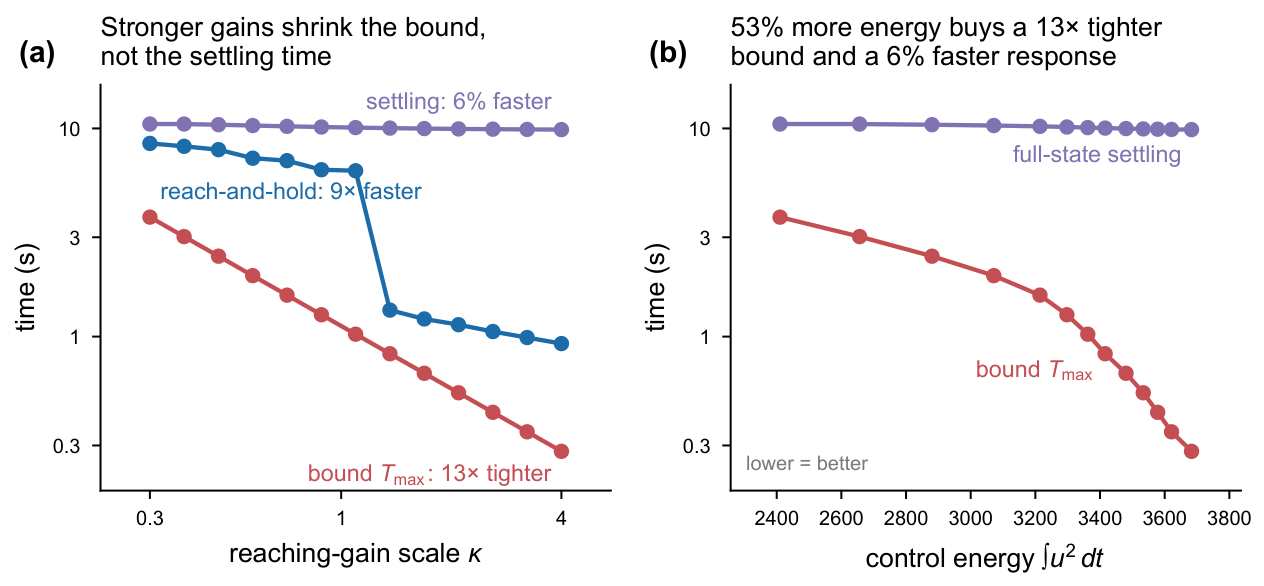
Figure 2.
Control energy versus full-state settling time for both controller families at three initial conditions, with each curve traced by the gain scale . The families overlap at matched settling time, so neither is systematically more efficient than the other on this benchmark.
Figure 2.
Control energy versus full-state settling time for both controller families at three initial conditions, with each curve traced by the gain scale . The families overlap at matched settling time, so neither is systematically more efficient than the other on this benchmark.
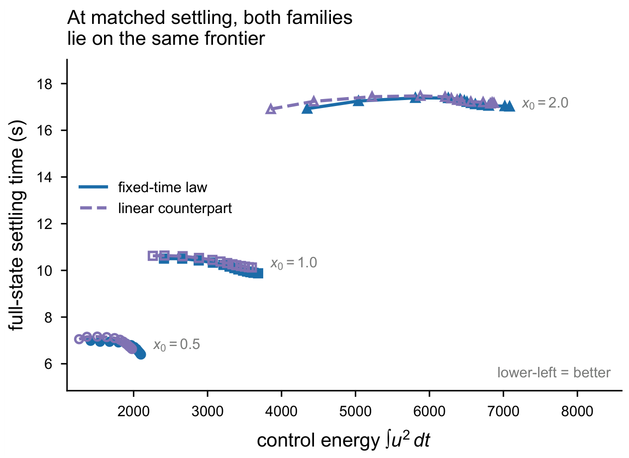
Figure 3.
The performance floor is not an artifact of actuator saturation. (a) Raising the virtual-acceleration clip improves settling until and then stops; the dashed line marks the saturation-free floor. (b) With the clip effectively removed (), a -fold gain range changes settling by only .
Figure 3.
The performance floor is not an artifact of actuator saturation. (a) Raising the virtual-acceleration clip improves settling until and then stops; the dashed line marks the saturation-free floor. (b) With the clip effectively removed (), a -fold gain range changes settling by only .
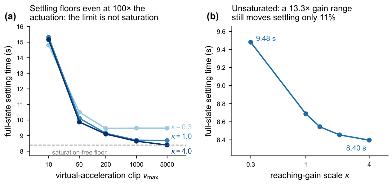
Figure 4.
The analytical bound is valid for the event it describes. (a) First-arrival time, reach-and-hold time, and the bound plotted against the gain scale; the bound tracks first arrival and lies well above it, while reach-and-hold follows a different law. (b) First arrival divided by the bound for both actuation regimes; every design lies below unity, so the certificate is honoured throughout, with margins between and .
Figure 4.
The analytical bound is valid for the event it describes. (a) First-arrival time, reach-and-hold time, and the bound plotted against the gain scale; the bound tracks first arrival and lies well above it, while reach-and-hold follows a different law. (b) First arrival divided by the bound for both actuation regimes; every design lies below unity, so the certificate is honoured throughout, with margins between and .
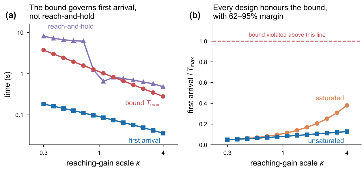
Figure 5.
Two tests of generality. (a) Coupling authority buys a real improvement in response: an eightfold increase yields a factor of in settling time while also reducing the energy integral. (b) The cart-pole benchmark shows the same separation more sharply, reaching the target times faster and settling flat to within .
Figure 5.
Two tests of generality. (a) Coupling authority buys a real improvement in response: an eightfold increase yields a factor of in settling time while also reducing the energy integral. (b) The cart-pole benchmark shows the same separation more sharply, reaching the target times faster and settling flat to within .
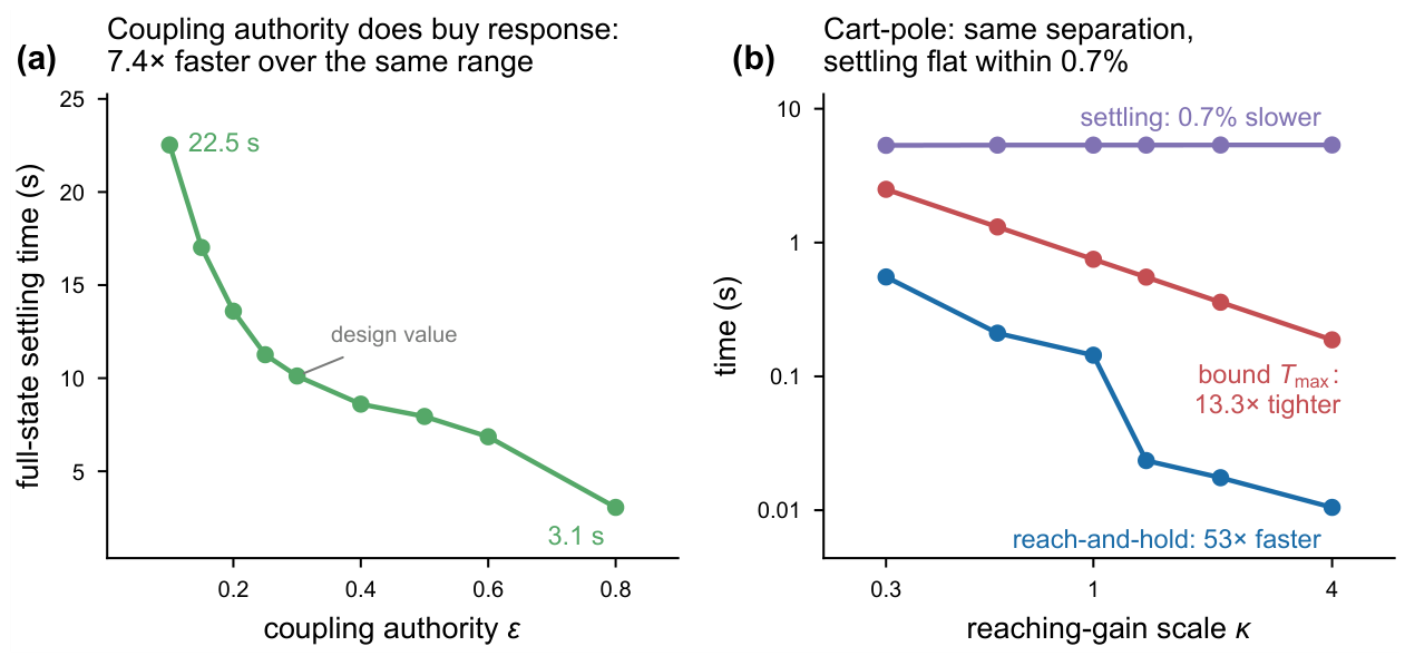
Figure 6.
Two-dimensional sweep over the reaching-gain scale and the fractional exponent , 49 designs. (a) Full-state settling time varies by across the grid and is banded almost entirely by . (b) The analytical bound over the same grid varies by a factor of .
Figure 6.
Two-dimensional sweep over the reaching-gain scale and the fractional exponent , 49 designs. (a) Full-state settling time varies by across the grid and is banded almost entirely by . (b) The analytical bound over the same grid varies by a factor of .
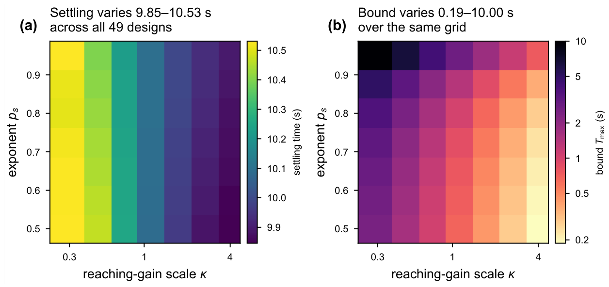
Figure 7.
Three sensitivity tests of the floor at , each over the full 13-point gain sweep. (a) Full-state settling at , , and tolerance bands; the band shifts every curve and changes none of their slopes. (b) Settling for true parameter vectors with ; the four curves coincide to within the line width. (c) Settling under a 1 s internal-acceleration pulse of amplitude A applied at s; the delay grows with the gains, so the highest-gain designs recover most slowly. The analytical bound tightens by across the horizontal range of every panel.
Figure 7.
Three sensitivity tests of the floor at , each over the full 13-point gain sweep. (a) Full-state settling at , , and tolerance bands; the band shifts every curve and changes none of their slopes. (b) Settling for true parameter vectors with ; the four curves coincide to within the line width. (c) Settling under a 1 s internal-acceleration pulse of amplitude A applied at s; the delay grows with the gains, so the highest-gain designs recover most slowly. The analytical bound tightens by across the horizontal range of every panel.
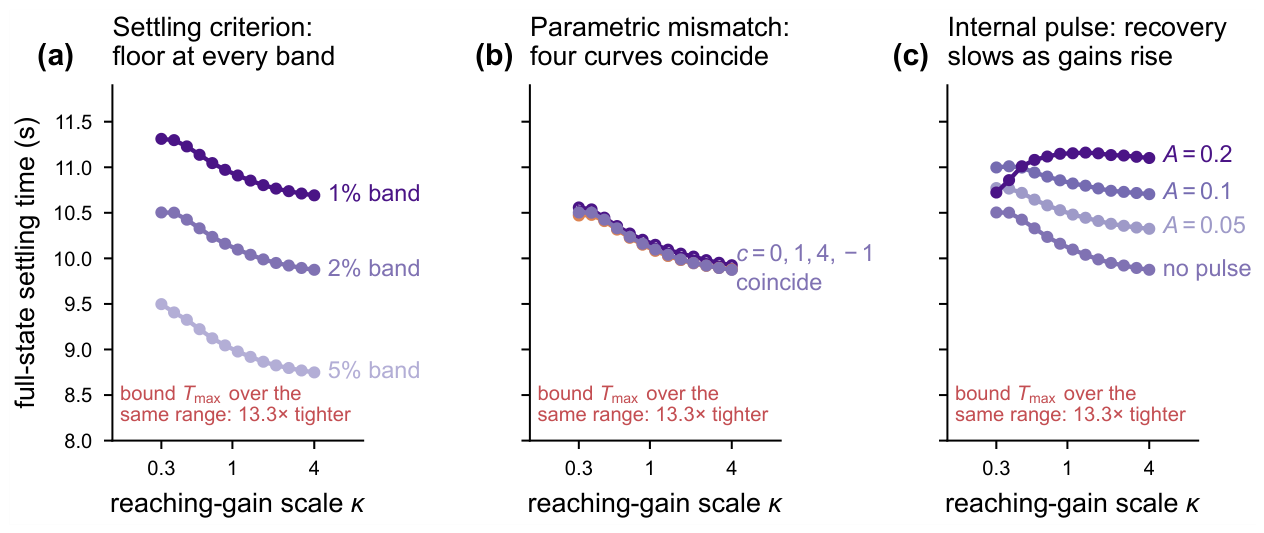
Figure 8.
(a) Full-state settling against the analytical bound for 150 designs varying all eight controller parameters, coloured by energy, with the one-parameter family of Table 6 overlaid. Settling is unrelated to the bound across a 40-fold range of the latter; the seven designs that settle faster than the family do so at 17 to 21 times its peak torque. (b) Torque chatter over the last 5 s of a sampled-data implementation as a function of the reaching-gain scale, for sample periods from 1 to 20 ms (log axis, with zero at the bottom). The high-gain designs chatter; the low-gain designs do not.
Figure 8.
(a) Full-state settling against the analytical bound for 150 designs varying all eight controller parameters, coloured by energy, with the one-parameter family of Table 6 overlaid. Settling is unrelated to the bound across a 40-fold range of the latter; the seven designs that settle faster than the family do so at 17 to 21 times its peak torque. (b) Torque chatter over the last 5 s of a sampled-data implementation as a function of the reaching-gain scale, for sample periods from 1 to 20 ms (log axis, with zero at the bottom). The high-gain designs chatter; the low-gain designs do not.
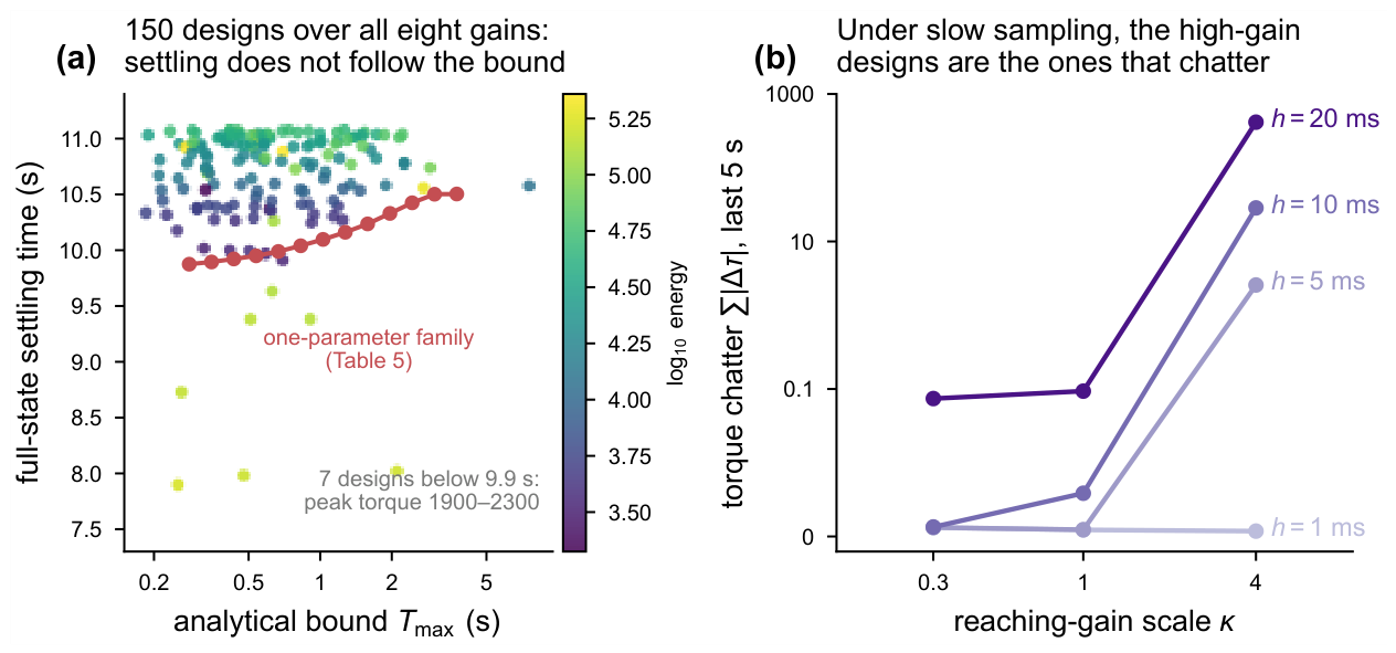
Table 1.
Division of labour between the two parts of the study. Shared material is confined to Section 3, where the plant, the controller equations, and the two theorem statements of Part 1 are cited rather than reproduced.
Table 1.
Division of labour between the two parts of the study. Shared material is confined to Section 3, where the plant, the controller equations, and the two theorem statements of Part 1 are cited rather than reproduced.
| Part 1 [1] | This paper | |
|---|---|---|
| Question | Can a fixed-time certificate be established for this class? | What does the certificate cost, and what does tightening it buy? |
| Object | One design, at one set of gains | A one-parameter family of designs, |
| Method | Synthesis and Lyapunov proof | Decomposition (4), Proposition 1, gain sweeps, matched-performance comparison (Section 4.7) |
| Main result | Two certificates: (2) and the internal-dynamics certificate | A structural floor on settling time (Proposition 1); certificate tightens while settling moves |
| Controls | none | Saturation relief, second benchmark, second gain direction, gain family outside the certificate, settling tolerance, parametric mismatch and adaptation gain, bounded disturbance, full gain space, sampled-data implementation, cost metric, grid resolution (Section 6) |
| Deliverable | The controller and its guarantees | A gain-selection rule (Section 5.6) |
| What is varied | Initial condition, at fixed gains | Gains, at fixed and at three initial conditions |
Table 4.
The internal energy at the first-arrival instant, , is constant to within across the sweep at , unlike the reach-and-hold time itself. This is the quantity that Proposition 1 shows converges to .
Table 4.
The internal energy at the first-arrival instant, , is constant to within across the sweep at , unlike the reach-and-hold time itself. This is the quantity that Proposition 1 shows converges to .
| (s) | ||
|---|---|---|
| 0.300 | 0.184 | 1.0014 |
| 0.573 | 0.127 | 1.0005 |
| 1.095 | 0.086 | 1.0002 |
| 1.359 | 0.075 | 1.0001 |
| 2.093 | 0.057 | 1.0001 |
| 4.000 | 0.036 | 1.0000 |
Table 5.
Reaching phase, measured by reach-and-hold, as a fraction of full-state settling time at the design gains ().
Table 5.
Reaching phase, measured by reach-and-hold, as a fraction of full-state settling time at the design gains ().
| reach-and-hold (s) | settling (s) | reaching share | |
|---|---|---|---|
| 0.5 | 3.225 | 6.750 | |
| 1.0 | 6.297 | 10.117 | |
| 2.0 | 14.041 | 17.239 |
Table 9.
Worked application of the selection rule at : the scale is read off (5) rather than searched for. Tightening the certificate by a factor of costs more energy and returns of settling time.
Table 9.
Worked application of the selection rule at : the scale is read off (5) rather than searched for. Tightening the certificate by a factor of costs more energy and returns of settling time.
| required | achieved | settling (s) | energy | |||
|---|---|---|---|---|---|---|
| 1.125 | 1.0000 | 8.00 | 4.00 | 1.1250 | 10.117 | 3348 |
| 0.600 | 1.8750 | 15.00 | 7.50 | 0.6000 | 9.967 | 3506 |
| 0.400 | 2.8125 | 22.50 | 11.25 | 0.4000 | 9.910 | 3603 |
| 0.250 | 4.5000 | 36.00 | 18.00 | 0.2500 | 9.868 | 3681 |
Table 10.
Effect of relaxing the virtual-acceleration clip at the design gains (, ). Settling ceases to improve beyond , while the energy integral continues to grow.
Table 10.
Effect of relaxing the virtual-acceleration clip at the design gains (, ). Settling ceases to improve beyond , while the energy integral continues to grow.
| settling (s) | energy | |
|---|---|---|
| 10 | 15.315 | 3461 |
| 50 | 10.117 | 3348 |
| 200 | 9.150 | 13219 |
| 1000 | 8.709 | 33428 |
| 5000 | 8.688 | 36575 |
| 20000 | 8.688 | 36575 |
Table 11.
Effect of relaxing the virtual-acceleration clip at and (design gains, ). Both initial conditions show the same saturation-free floor pattern as Table 10.
Table 11.
Effect of relaxing the virtual-acceleration clip at and (design gains, ). Both initial conditions show the same saturation-free floor pattern as Table 10.
| settling (s) | ||
|---|---|---|
| 10 | 7.384 | 20.337 |
| 50 | 6.750 | 17.239 |
| 200 | 5.398 | 16.420 |
| 1000 | 5.135 | 15.750 |
| 5000 | 5.135 | 15.582 |
| 20000 | 5.135 | 15.582 |
Table 12.
Full-state settling time versus reaching-gain scale, with the actuator limit effectively removed (, ). The floor persists: the same gain range that tightens the bound by changes the settling time by .
Table 12.
Full-state settling time versus reaching-gain scale, with the actuator limit effectively removed (, ). The floor persists: the same gain range that tightens the bound by changes the settling time by .
| settling, unsaturated (s) | |
|---|---|
| 0.300 | 9.481 |
| 1.000 | 8.688 |
| 1.359 | 8.545 |
| 2.093 | 8.455 |
| 4.000 | 8.397 |
Table 15.
Full-state settling time and control energy versus the coupling authority , at the design gains (, ). Unlike the reaching gains, improves the response while also reducing the energy integral. The value is the design value used elsewhere in the paper.
Table 15.
Full-state settling time and control energy versus the coupling authority , at the design gains (, ). Unlike the reaching gains, improves the response while also reducing the energy integral. The value is the design value used elsewhere in the paper.
| settling (s) | energy | |
|---|---|---|
| 0.10 | 22.528 | 9707 |
| 0.15 | 17.021 | 7071 |
| 0.20 | 13.600 | 5054 |
| 0.25 | 11.261 | 4197 |
| 0.30 | 10.117 | 3348 |
| 0.40 | 8.607 | 3196 |
| 0.50 | 7.944 | 1911 |
| 0.60 | 6.854 | 1274 |
| 0.80 | 3.060 | 665 |
Table 16.
Gain sweep on the cart-pole benchmark (), reported to four decimal places so the factors quoted in the text reproduce exactly. The bound and manifold reaching time respond strongly to the gains, whereas the full-state settling time varies by less than , becoming marginally slower.
Table 16.
Gain sweep on the cart-pole benchmark (), reported to four decimal places so the factors quoted in the text reproduce exactly. The bound and manifold reaching time respond strongly to the gains, whereas the full-state settling time varies by less than , becoming marginally slower.
| (s) | reach-and-hold (s) | settling (s) | energy | |
|---|---|---|---|---|
| 0.300 | 2.5000 | 0.5535 | 5.3285 | 0.3304 |
| 0.573 | 1.3089 | 0.2105 | 5.3495 | 0.5649 |
| 1.000 | 0.7500 | 0.1440 | 5.3500 | 0.9938 |
| 1.359 | 0.5519 | 0.0235 | 5.3520 | 1.3799 |
| 2.093 | 0.3583 | 0.0175 | 5.3600 | 2.2034 |
| 4.000 | 0.1875 | 0.0105 | 5.3650 | 4.4291 |
Table 17.
Settling time and control energy against the outer-loop gain scale , with the reaching-law gains fixed (, ). Unlike (5), does not appear in the certificate (2) at all.
| settling (s) | energy | |
|---|---|---|
| 0.300 | 9.084 | 1169 |
| 0.372 | 7.442 | 1094 |
| 0.462 | 8.112 | 1647 |
| 0.573 | 8.982 | 2636 |
| 0.711 | 9.315 | 4225 |
| 0.883 | 9.878 | 3291 |
| 1.095 | 10.287 | 3575 |
| 1.359 | 10.742 | 5008 |
| 1.687 | 10.805 | 4341 |
| 2.093 | 10.876 | 4205 |
| 2.598 | 10.873 | 4274 |
| 3.223 | 10.737 | 5623 |
| 4.000 | 31.653 | 108088 |
Table 18.
Sensitivity of the headline result to the settling criterion. Full-state settling time at the two ends of the reaching-gain sweep, and , for tolerance bands of , (the value used elsewhere in the paper), and , at three initial conditions. The analytical bound tightens by a factor of across every row. The reach-and-hold time is defined on the sliding variable ( for s) and does not depend on the band.
Table 18.
Sensitivity of the headline result to the settling criterion. Full-state settling time at the two ends of the reaching-gain sweep, and , for tolerance bands of , (the value used elsewhere in the paper), and , at three initial conditions. The analytical bound tightens by a factor of across every row. The reach-and-hold time is defined on the sliding variable ( for s) and does not depend on the band.
| band | settling (s) | reach-and-hold (s) | ||||
|---|---|---|---|---|---|---|
| change | ||||||
| 0.5 | 7.677 | 7.213 | 5.986 | 0.901 | ||
| 1.0 | 11.312 | 10.692 | 8.475 | 0.926 | ||
| 2.0 | 17.711 | 17.836 | 15.223 | 0.939 | ||
| 0.5 | 6.985 | 6.397 | 5.986 | 0.901 | ||
| 1.0 | 10.504 | 9.875 | 8.475 | 0.926 | ||
| 2.0 | 16.927 | 17.021 | 15.223 | 0.939 | ||
| 0.5 | 5.774 | 5.270 | 5.986 | 0.901 | ||
| 1.0 | 9.498 | 8.749 | 8.475 | 0.926 | ||
| 2.0 | 15.825 | 15.897 | 15.223 | 0.939 | ||
Table 19.
Sensitivity to parametric mismatch and adaptation gain, . Upper block: the true parameter vector is , so is no uncertainty, the value used elsewhere in the paper, four times the design mismatch, and the sign-reversed vector; throughout. Lower block: adaptation gain varied at . Settling is the full-state criterion; reach-and-hold is held for s, with n/r meaning not reached within the 20 s horizon; energy is at . The bound tightens by across every row.
Table 19.
Sensitivity to parametric mismatch and adaptation gain, . Upper block: the true parameter vector is , so is no uncertainty, the value used elsewhere in the paper, four times the design mismatch, and the sign-reversed vector; throughout. Lower block: adaptation gain varied at . Settling is the full-state criterion; reach-and-hold is held for s, with n/r meaning not reached within the 20 s horizon; energy is at . The bound tightens by across every row.
| settling (s) | reach-and-hold (s) | energy | |||||
|---|---|---|---|---|---|---|---|
| change | |||||||
| 10.486 | 10.112 | 9.875 | 8.473 | 0.902 | 3704 | ||
| 10.495 | 10.113 | 9.875 | 8.473 | 0.915 | 3688 | ||
| 10.504 | 10.117 | 9.875 | 8.475 | 0.926 | 3683 | ||
| 10.519 | 10.131 | 9.879 | 8.478 | 0.948 | 3659 | ||
| 10.559 | 10.169 | 9.925 | 8.486 | 0.965 | 3672 | ||
| 10.471 | 10.106 | 9.880 | 8.471 | 0.789 | 3759 | ||
| 11.559 | 10.402 | 10.407 | n/r | 0.842 | 3106 | ||
| 10.504 | 10.117 | 9.875 | 8.475 | 0.926 | 3683 | ||
| 11.063 | 10.457 | 10.200 | 8.115 | 1.754 | 6722 | ||
Table 20.
Bounded disturbances, . Upper block: a rectangular pulse of amplitude A on s, applied after first arrival so that it perturbs the plant-governed phase directly, added to the internal-coordinate acceleration (“internal”) or to the actuated channel (“actuated”); settling is the full-state criterion and energy is at . Lower block: a persistent sinusoid on the same channels; the full state no longer re-enters the band because the actuated angle must move to reject the disturbance, so the ultimate bounds of and over the last 5 s are reported instead, with energy at both ends of the sweep. The bound tightens by across every row.
Table 20.
Bounded disturbances, . Upper block: a rectangular pulse of amplitude A on s, applied after first arrival so that it perturbs the plant-governed phase directly, added to the internal-coordinate acceleration (“internal”) or to the actuated channel (“actuated”); settling is the full-state criterion and energy is at . Lower block: a persistent sinusoid on the same channels; the full state no longer re-enters the band because the actuated angle must move to reject the disturbance, so the ultimate bounds of and over the last 5 s are reported instead, with energy at both ends of the sweep. The bound tightens by across every row.
| Pulse disturbance | |||||||||
|---|---|---|---|---|---|---|---|---|---|
| channel | settling (s) | change | energy | ||||||
| none | – | 10.504 | 10.117 | 9.875 | 3683 | ||||
| internal | 0.05 | 10.772 | 10.504 | 10.325 | 3716 | ||||
| internal | 0.10 | 10.998 | 10.840 | 10.705 | 4050 | ||||
| internal | 0.20 | 10.723 | 11.154 | 11.102 | 4505 | ||||
| actuated | 0.10 | 10.507 | 10.120 | 9.877 | 3681 | ||||
| Persistent sinusoidal disturbance | |||||||||
| channel | ultimate bound of | ult. bound of | energy | ||||||
| change | |||||||||
| internal | 0.05 | 0.0074 | 0.0069 | 0.0068 | 0.20 | 0.18 | 2713 | 3930 | |
| internal | 0.10 | 0.0163 | 0.0154 | 0.0150 | 0.38 | 0.37 | 2739 | 4320 | |
| internal | 0.20 | 0.0290 | 0.0255 | 0.0251 | 1.13 | 1.08 | 5569 | 10288 | |
| actuated | 0.10 | 0.0000 | 0.0000 | 0.0000 | – | 0.0004 | 0.0001 | 2423 | 3673 |
Table 21.
Search over the full gain space, : 150 Latin-hypercube designs varying all six reaching and surface gains over their design values and both exponents (, ). Upper block: Spearman rank correlation of full-state settling time and of log energy with each parameter. Lower block: cheapest design that meets a settling threshold, in the one-parameter family of Table 6 and in the full space, with its peak torque. Across the 150 designs the bound spans a factor of 40 and settling spans to s.
Table 21.
Search over the full gain space, : 150 Latin-hypercube designs varying all six reaching and surface gains over their design values and both exponents (, ). Upper block: Spearman rank correlation of full-state settling time and of log energy with each parameter. Lower block: cheapest design that meets a settling threshold, in the one-parameter family of Table 6 and in the full space, with its peak torque. Across the 150 designs the bound spans a factor of 40 and settling spans to s.
| parameter | (settling) | (log energy) | |||
|---|---|---|---|---|---|
| (reaching) | |||||
| (reaching) | |||||
| (reaching) | |||||
| (reaching exponent) | |||||
| (reaching exponent) | |||||
| (surface) | |||||
| (surface) | |||||
| (surface) | |||||
| one-parameter family | full gain space | ||||
| threshold | energy | energy | saving | ||
| s | 2880 | 72 | 2229 | 89 | -23% |
| s | 3362 | 91 | 3163 | 118 | -6% |
| s | 3621 | 105 | 129081 | 1875 | +3465% |
| s | none | – | 129081 | 1875 | – |
Table 22.
Sampled-data implementation, . The controller reads the state every h seconds, with additive Gaussian measurement noise of standard deviation on every state, computes the torque once per sample, quantizes it to steps of q where stated, and holds it; the plant integrates continuously and the adaptation law is updated at the sample instants. Upper block: cases in which the full-state band is reached; chatter is the total variation of the torque over the last 5 s, and energy is at . Lower block: cases in which the noise-driven motion of exceeds the rad band, so the ultimate bounds of and over the last 5 s are reported instead, with energy at both ends of the sweep. Noise rows are means over three noise realizations. The bound tightens by across every row.
Table 22.
Sampled-data implementation, . The controller reads the state every h seconds, with additive Gaussian measurement noise of standard deviation on every state, computes the torque once per sample, quantizes it to steps of q where stated, and holds it; the plant integrates continuously and the adaptation law is updated at the sample instants. Upper block: cases in which the full-state band is reached; chatter is the total variation of the torque over the last 5 s, and energy is at . Lower block: cases in which the noise-driven motion of exceeds the rad band, so the ultimate bounds of and over the last 5 s are reported instead, with energy at both ends of the sweep. Noise rows are means over three noise realizations. The bound tightens by across every row.
| settling (s) | chatter | energy | ||||||
|---|---|---|---|---|---|---|---|---|
| implementation | change | |||||||
| ms | 10.509 | 10.126 | 9.881 | 0.00 | 0.00 | 3660 | ||
| ms | 10.517 | 10.152 | 9.916 | 0.00 | 2.57 | 3646 | ||
| ms | 10.556 | 10.181 | 9.982 | 0.00 | 28.54 | 3614 | ||
| ms | 10.642 | 10.274 | 10.022 | 0.07 | 415.01 | 3994 | ||
| , ms | 10.605 | 10.265 | 10.163 | 1368.43 | 21354.72 | 7391 | ||
| , ms | 10.532 | 10.151 | 9.916 | 9.00 | 22.00 | 3647 | ||
| , ms | 10.544 | 10.139 | 9.913 | 26.00 | 129.00 | 3651 | ||
| ultimate bound of | ult. bound of | energy | ||||||
| implementation | change | |||||||
| , ms | 0.0013 | 0.0012 | 0.0012 | 0.069 | 0.085 | 3569 | 27931 | |
| , ms, | 0.0018 | 0.0019 | 0.0025 | 0.089 | 0.111 | 3454 | 28665 | |
Table 23.
Matched-performance comparison of the fixed-time law with its linear counterpart under four cost metrics: the energy used elsewhere in the paper, the absolute effort , the total variation (an actuator-wear proxy), and the peak torque . Each entry is the ratio fixed-time/linear of the smallest cost attained by any sweep point that settles at least as fast as the common target, by the protocol of Section 4.7. A ratio below one favours the fixed-time law.
Table 23.
Matched-performance comparison of the fixed-time law with its linear counterpart under four cost metrics: the energy used elsewhere in the paper, the absolute effort , the total variation (an actuator-wear proxy), and the peak torque . Each entry is the ratio fixed-time/linear of the smallest cost attained by any sweep point that settles at least as fast as the common target, by the protocol of Section 4.7. A ratio below one favours the fixed-time law.
| target (s) | |||||
|---|---|---|---|---|---|
| 0.5 | 6.634 | 1.041 | 1.023 | 0.978 | 0.926 |
| 1.0 | 10.124 | 0.934 | 0.982 | 0.905 | 0.842 |
| 2.0 | 16.927 | 1.128 | 1.043 | 1.077 | 1.074 |
Table 24.
Matched-performance energies from the 13-point sweep used throughout the paper and from a 49-point sweep over the same range , both families, three initial conditions. The common settling target is identical on both grids. The energy ratio moves by at most .
Table 24.
Matched-performance energies from the 13-point sweep used throughout the paper and from a 49-point sweep over the same range , both families, three initial conditions. The common settling target is identical on both grids. The energy ratio moves by at most .
| fixed-time energy | linear energy | ratio | ||||
|---|---|---|---|---|---|---|
| 13 pts | 49 pts | 13 pts | 49 pts | 13 pts | 49 pts | |
| 0.5 | 2059 | 2046 | 1977 | 1977 | 1.041 | 1.035 |
| 1.0 | 3362 | 3347 | 3599 | 3599 | 0.934 | 0.930 |
| 2.0 | 4346 | 4346 | 3854 | 3854 | 1.128 | 1.128 |
Disclaimer/Publisher’s Note: The statements, opinions and data contained in all publications are solely those of the individual author(s) and contributor(s) and not of MDPI and/or the editor(s). MDPI and/or the editor(s) disclaim responsibility for any injury to people or property resulting from any ideas, methods, instructions or products referred to in the content. |
© 2026 by the authors. Licensee MDPI, Basel, Switzerland. This article is an open access article distributed under the terms and conditions of the Creative Commons Attribution (CC BY) license (http://creativecommons.org/licenses/by/4.0/).
Copyright: This open access article is published under a Creative Commons CC BY 4.0 license, which permit the free download, distribution, and reuse, provided that the author and preprint are cited in any reuse.