
Submitted:
27 September 2026
Posted:
29 September 2026
You are already at the latest version
Abstract
Cybersecurity incidents can disrupt voltage regulation even when controller inputs pass basic validity checks. This study evaluates their effects and the conditions for effective local backup regulation in a reference 110/15 kV substation. A balanced AC power flow model is coupled with a discrete on-load tap changer (OLTC) model. The system comprises two 25 MVA transformers, six feeders and 18 load buses. Two control architectures and four protection strategies are compared using a 6990-trial protocol, including series with 30 random realizations per variant. In the main incident matrix, voltage-band violations occurred in 9 of 225 unprotected incident trials per architecture. Strategies R1 and R2 prevented these violations; R2 reduced tap changes by 43.1% relative to R1. With the same detector, backup regulation R2 reduced voltage-profile degradation compared with command blocking R2B. For telemetry delays up to 8 s, the mean paired difference in the increase in integrated voltage deviation was −91.946 p.u.·s (95% confidence interval: [−98.756, −85.136] p.u.·s). However, brief recurring anomalies could trigger alarms without activating backup regulation, while similar errors in both measurement channels remained undetected. Protection assessment therefore requires joint analysis of detection, response timing and retained regulation capability, accounting for backup-channel trustworthiness.
Keywords:
110/15 kV substation
; OT cybersecurity
; voltage regulation
; on-load tap changer
; false data injection
; replay attack
; local backup regulation
1. Introduction
Digital control of a primary substation requires consideration of communication availability, measurement trustworthiness and the timing constraints of tap-changing voltage regulation. A falsified measurement may remain within the admissible range, while an unauthorized setpoint change may produce commands that comply with the controller algorithm but conflict with the control objective. Communication availability alone is therefore insufficient to determine the physical consequences of an incident. This study quantitatively evaluates these consequences in a reference 110/15 kV substation and identifies the conditions under which data validation and local backup regulation improve voltage regulation performance.
Physical protection of equipment, network segmentation and cryptographic protection of communications constitute layers of operational technology (OT) security [1]. However, these mechanisms do not ensure the correctness of data generated by a sensor or controller compromised by an attacker. This motivates checking measurement consistency with the physical process and analyzing the response of the entire control loop. The present study uses deterministic data-validation mechanisms; artificial intelligence (AI) methods are reserved for future research.
1.1. Related Work
Isozaki et al. [2] investigated cyberattack detection for voltage control in distribution networks with photovoltaic generation. AlMajali et al. [3] studied the effects of tap-changer manipulation, load changes and photovoltaic generation on distribution-system voltages using a real-time simulator. These studies provide a basis for examining the relationship between manipulation of data or control actions and the electrical response of the network. The present study assesses the entire voltage control loop during an incident, including the on-load tap changer (OLTC) as the actuator.
Within the OT security framework described by NIST [1], the assessment of protective mechanisms should account for process reliability and safety requirements. Blocking new commands may limit unwanted tap changes but degrade regulation under varying supply conditions. Accordingly, this study compares command blocking with preservation of voltage regulation through a backup channel.
The publications examined from 2023–2026 address the physical consequences of false data injection (FDI), mitigation through control of network resources, and AI-based detection and control. Bragatto et al. [4] considered the effects of FDI on centralized voltage regulation in systems with high penetration of renewable energy sources (RES). Naderi and Asrari [5,6,7] analyzed attack mitigation through reactive power control, network reconfiguration and load management. Selim et al. [8], Zhang [9] and Ang et al. [10] presented machine-learning-based approaches, whereas Li et al. [11] employed robust model predictive control. These methods differ in their actuators, network topologies and control time scales.
Table 1 summarizes the scope of the related studies and their relationship to the present work. The comparison draws on the methods and results reported by the authors, without rerunning their experiments. Because the models and metrics differ, the percentage improvements reported in the literature are not directly compared with the reduction in tap changes in the present trial set.
The most closely related studies concern attacks on on-load tap changers, also denoted by ULTC and LTC in the literature [3,6], and distributed energy resource management systems (DERMS) [12]. In these studies, manipulation of data or commands affects voltages and voltage-regulating devices. The present results are qualitatively consistent with this mechanism. The comparative contribution is to identify conditions under which detection does not produce an effective response, and to assess the degradation caused by command blocking relative to backup regulation. No performance comparison was conducted with published algorithms implemented in a common test environment. The hardware-in-the-loop (HIL) dataset developed by Cibin et al. [13] suggests how validation could be extended to intelligent electronic device (IED) telemetry and actual communication traffic.
1.2. Specific Objective and Contribution
This work compares two control architectures and four defined protection strategies within a common closed-loop model. The main matrix includes R0, R1 and R2, while the extension introduces R2B, which uses the same detector and the same activation and return delays as R2. R2B blocks new commands, whereas R2 transfers regulation to a backup channel. This comparison isolates the effect of the response to a detected anomaly on the retention of voltage regulation capability. The analysis also covers the detection boundary, communication irregularities, nonmalicious faults and partial loss of measurement independence. All variants are compared against reference runs using the same realizations of random disturbances.
Three research questions are addressed. The first concerns the effects of the sign and magnitude of the injected modification and the incident duration on actual load-bus voltages and the number of tap changes. The second concerns differences between a centralized control loop that depends on remote communications and a local controller supervised by SCADA. The third concerns the conditions for effective operation and the limitations of an independent measurement used with local backup regulation. Assessment is relative to paired runs without an incident, with identical load profiles and random-disturbance realizations.
Switching-operation analysis is limited to tap-change sequences, time delays, blocking and control transfer. This scope allows the effects of incidents on voltage regulation to be studied but excludes commutation phenomena and wear of tap-changer components.
2. Materials and Methods
2.1. Reference Substation Model
The model represents a reference system rather than a specific Energa-Operator substation. The operator’s public standard [14] describes voltage-control functions but does not establish how frequently particular controller models are used. Documented functions of a reference controller were therefore adopted without assuming that it predominates in the operator’s installations. The trials concern a functional model and do not constitute vulnerability testing of a particular manufacturer’s device.
The system comprises two medium-voltage (MV) busbar sections with an open bus coupler. Each transformer supplies three radial feeders, each containing three load buses. The sections are supplied by independent stiff high-voltage (HV) sources with the same prescribed voltage profile. The model excludes a common 110 kV network impedance and parallel transformer operation. The topology contains 18 load buses and two MV busbars. Component parameters are listed in Table 2.
Figure 1.
Topology of the simulated substation. ZK labels identify load buses; bus coupler QS remains open. OLTC: on-load tap changer.
Figure 1.
Topology of the simulated substation. ZK labels identify load buses; bus coupler QS remains open. OLTC: on-load tap changer.
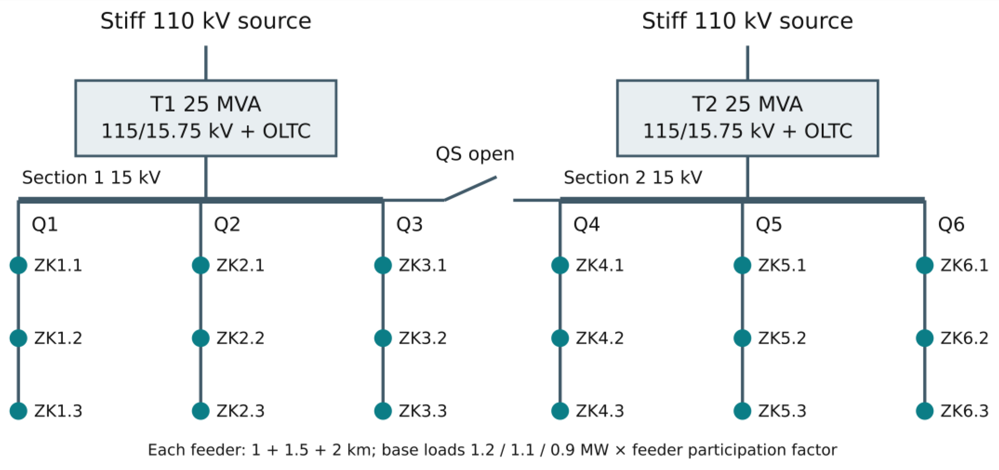
The total base active load is 19.2 MW. Load scaling factors of 0.6, 1.0 and 1.4 multiply the base power profile; they do not denote percentage transformer loading. Different feeder participation factors reduce the symmetry of load-bus voltages. Cable resistance is assumed constant at a conductor temperature of 90 °C. For three single-core cables installed in trefoil, the manufacturer’s current rating is 525 A at a burial depth of 0.7 m, a ground temperature of 20 °C, a soil thermal resistivity of 1 K·m/W and bonding of the screens at both ends (BE) [16] (pp. 28–30). The value of 516 A applies to a flat arrangement. These current ratings are used solely as manufacturer reference values and do not replace a thermal analysis.
2.1.1. Network Equations and Physical Parameters
Calculations assume a balanced three-phase system, constant active and reactive power (PQ) loads, and π-equivalent circuits for cable sections. A three-phase power base of 25 MVA and an MV-side line-to-line voltage base of 15 kV are used. The rated winding voltages of 115/15.75 kV are distinguished from the nominal network voltages of 110/15 kV. For tap position n, the ideal MV-side source voltage in per-unit (p.u.) notation is:
In Equation (1), usrc(t) is the HV source voltage referred to 110 kV. Increasing n decreases the MV-side voltage. Transformer impedance is derived from the short-circuit voltage and load losses and referred to the rated lower-voltage winding voltage. A constant leakage impedance is placed behind the ideal transformer ratio. No-load losses are represented by a conductance; the reactive component of the magnetizing current is omitted because no no-load current data are available. The YNd11 vector group does not affect the calculated voltage magnitudes in this balanced model, with separate section operation and zero-sequence quantities excluded. In Equation (2), Pk denotes load losses, ULV the rated lower-voltage winding voltage, Sn rated apparent power, and uk the percentage short-circuit voltage; Rk, Xk and Zk are the equivalent short-circuit impedance parameters.
Power flow is solved by current–voltage iteration for the radial network. Per-unit load currents follow i = (s/v)*, with a three-phase power base Sb = 25 MVA, a line-to-line voltage base Ub,LL = 15 kV and a current base Ib = Sb/(√3 Ub,LL). In SI phasor notation, the relationship is Iφ = [S3φ/(3Vφ)]*, and the magnitudes satisfy |S3φ| = √3 ULL |I|. The asterisk denotes complex conjugation. Capacitive currents in the shunt branches of the π-equivalent circuits are included. Iteration terminates when the maximum change in complex voltage is below 10−11 p.u., subject to a limit of 100 iterations. Nonconvergent trials are classified as invalid. To reduce computation time, solutions for all 25 admissible tap positions are calculated at each instant, retaining the stated numerical tolerance and without interpolation between taps. The controller selects the solution corresponding to the current OLTC position.
At the initial instant, with a load scaling factor of 1.0 and tap position −1, the section 1 busbar voltage is 14.9878 kV and the MV-side current of T1 is 388.226 A. The power on that side is P = 9.64309 MW and Q = 2.92930 Mvar, giving |S| = 10.07819 MVA, consistent with √3 ULL I. The total load of both sections is 19.2 MW and the power drawn from the sources is 19.36395 MW; the difference of 0.16395 MW represents model losses. These values are operating powers, not transformer ratings.
An ideal closed switch has zero voltage drop, and its current follows from the power flow in the corresponding branch. No current flows through the open bus coupler QS in this model. The voltage across its terminals is the difference between the phase voltages of the two sections, not the line-to-line voltage of a single busbar. With consistent phasor references, its magnitude across one pole is |Vφ1 − Vφ2|; busbar voltage magnitudes alone are insufficient without the phase-angle difference. Because the sources of the two sections are independent, the actual voltage across the open QS contacts cannot be determined without defining their relative phase. Voltages across the internal OLTC contacts are not calculated because the model does not include its commutation circuit or electromagnetic transients.
2.2. Load Profile
Each run spans 3600 s with a default time step of 1 s. The common load multiplier takes the values in Table 3, with linear interpolation between the listed intervals. At t = 0, the admissible tap position minimizing the busbar voltage deviation from 1 p.u. is selected. Tap changes associated with initialization are excluded from the operation count. Incident runs and their corresponding reference runs are identical before the incident starts.
In the Monte Carlo analysis, the load profile includes a random multiplier shared by each pair of runs, as described in Section 2.5. Excluding distributed generation and assuming zero HV source impedance limit the interpretation of the results to the defined load-supply system.
2.3. Control Architectures
Centralized and local architectures are compared; they differ in the location of the closed control loop and their dependence on remote channels. Supervisory control and data acquisition (SCADA) provides supervisory functions in both variants.
In the centralized architecture, the section 1 voltage measurement and the OLTC commands for T1 are transmitted over remote channels. In the local architecture, the controller uses a local measurement input and a local connection to the drive, while SCADA provides supervision and transmits the setpoint. Loss of a remote channel does not interrupt the local control loop. However, falsification at the measurement source can affect both architectures; it is not restricted to changing the value displayed on the operator interface. Transformer T2 is not directly affected by the incident and regulates the voltage of its own section.
2.4. Controller, Protection Strategies and Incident Model
The controller regulates the MV busbar voltage around a setpoint of 1 p.u., with a deadband of ±0.01 p.u. After the voltage remains continuously outside the deadband for 40 s, it commands a one-step tap change, with an execution time of 5 s. Each subsequent operation requires the full delay to elapse again. Re-entry into the deadband or a change in the sign of the control error resets the timer. A mechanical operation already in progress is completed even if control transfers to the backup channel. Tap-position limits are enforced. The deadband and definite-time delay functions are described in the TAPCON 260 documentation [17]; the drive operating time and specific settings are study assumptions. The model does not reproduce the device’s complete firmware. The protection strategies are summarized in Table 4.
The backup regulation channel uses its own measurement, an independent connection to the drive and an approved setpoint. Loss of the backup measurement blocks new T1 tap-change commands. Comparison of two measurement channels cannot ensure detection when both are falsified consistently. An alarm indicates a detected anomaly but does not identify its cause; a sensor fault may produce an analogous symptom. The incidents considered are listed in Table 5.
Algorithm 1 specifies the operations performed for T1 at each time step. It distinguishes the anomaly signal q, immediate inhibition of new commands, and the active backup state in R2 or blocking state in R2B. A measurement-discrepancy alarm alone does not stop primary regulation before the activation delay has elapsed, provided that the measurement remains valid and the command channel is available.
Algorithm 1. Update of the T1 controller and protection strategies.
1. Complete any previously initiated OLTC operation whose execution time has elapsed. Update the tap position, then calculate voltages for that position and the current load. Generate noisy measurements and apply the defined signal and communication modifications.
2. Check measurement availability and the admissible range [0.7, 1.3] p.u.; flag a message age > 3 s, a timestamp more than one time step ahead of the current time, or a sequence number below the largest previously received. Check the setpoint range [0.97, 1.03] p.u. and whether the time since the last command-channel heartbeat exceeds 3 s. For R2 and R2B, also check the availability of both measurements and the condition |uₚ − uᵣ| > 0.02 + 10−12 p.u.
3. Set q to the logical OR of the basic anomalies for R1 and, for R2 and R2B, also the measurement-comparison anomalies. Set q = 0 in R0. In R2 and R2B only: if q = 1, reset the healthy-data timer and start or continue timing the uninterrupted anomaly. If backup regulation or blocking is inactive, activate it after at least 5 s and reset the controller-delay timer once on this transition.
4. In R2 and R2B, if q = 0, reset the anomaly timer. While backup regulation or blocking is active, start or continue timing the period of valid data. After at least 60 s, restore the primary channel and reset the controller-delay timer once on this transition. A recurrence of q = 1 interrupts the return timer.
5. In R1, R2 and R2B, reject any setpoint outside the allowed range and use the approved value of 1 p.u. With R2 backup regulation active, select the backup measurement and the local drive connection; loss of that measurement inhibits new commands. With R2B blocking active, inhibit new commands. Issuing commands through the primary channel requires command-channel availability and, in the protected strategies, a valid measurement; R2 and R2B additionally require the backup measurement to be present.
6. Do not issue another command while an OLTC operation is in progress. Reset the controller timer when commands are inhibited, the measurement is absent, the error returns to the deadband, or no further admissible tap position exists. Restart timing when the error changes sign. After at least 40 s of uninterrupted error of the same sign outside the ±0.01 p.u. deadband, command a one-step tap change to be completed after 5 s. Record the alarm, control state and time-step results.
The 3 s and 5 s intervals are measured from different events: the last correctly received signal and the first time step with q = 1, respectively. Loss of the command channel inhibits new commands immediately, whereas the watchdog alarm occurs after the permitted signal age is exceeded. Any mechanical operation already in progress is completed. The event class assigned in the protocol is not a detector input.
Variants with refreshed timestamps assume access to the message source; they do not imply that cryptographic protection has been broken. Incidents are represented by defined modifications to simulation inputs. The model neither interacts with real infrastructure nor implements message exchange using IEC 60870-5-104, IEC 61850 or Modbus.
2.5. Experimental Design and Random Realizations
In the main matrix, the incident starts at 600 s and lasts 30, 120 or 600 s. For each duration, 20 basic cases are defined: six FDI variants, six setpoint changes, six replay attacks and two communication-channel outages. Five extended cases are added: FDI of +0.05 p.u. combined with a setpoint change of −0.05 p.u.; replay of a 120 s history with refreshed timestamps and loss of the command channel; FDI of +0.05 p.u. with loss of the backup measurement; consistent FDI of +0.05 p.u. in both channels; and loss of wide area network (WAN) connectivity. In total, 75 incident cases and one reference case are defined. This set does not exhaust possible substation attack scenarios. The sizes of all simulation series are listed in Table 6.
The initial Monte Carlo analysis uses pseudorandom number generator seeds 1001–1030. Measurement noise follows N(0, 0.0012) p.u. The load multiplier equals 1 plus interpolated perturbations sampled every 30 s from N(0, 0.0252), with the resulting multiplier clipped to [0.9, 1.1]. The incident start time is shifted by an integer number of seconds in [−90, 90]. The six cases comprise the incident-free reference, FDI of +0.05 p.u., a setpoint change of −0.10 p.u., replay of a 120 s history with refreshed timestamps, combined FDI and setpoint manipulation, and falsification of both measurements. The incident lasts 600 s. For a given seed, identical disturbance realizations are used in all compared variants.
Additive measurement noise is sampled independently for the primary T1 channel, the backup T1 channel and the T2 controller, and across simulation instants, without introducing cross-channel or temporal correlation into the source samples. Delay, holding and replay of measurements may subsequently introduce temporal dependence into the received signal. For seed s, NumPy Generator(PCG64), initialized through default_rng, uses s for the load profile, s + 104729 for noise, and s + 400109 for communication delays. The incident-start shift is sampled from a discrete uniform distribution over {−90, …, 90} s after reinitialization with seed s. Independence between this shift and the load-profile realization is therefore not assumed. The same disturbance-generation procedure is retained for all compared strategies and their reference runs.
The Monte Carlo analysis comprises 30 random realizations per variant at a load scaling factor of 1.0. The unit of statistical analysis is a complete realization identified by its generator seed, and the difference in metrics calculated for paired runs. Buses and successive time samples from the same run are not treated as independent observations. Means are accompanied by 95% confidence intervals based on Student’s t-distribution. The sample size defines the scope of an exploratory study; no statistical power analysis or estimation of real-world incident probabilities is performed.
2.6. Evaluation Metrics
The primary metric is the sum of the time integrals of violations of the adopted voltage band at the 18 load buses, calculated from the incident start time tₐ to the end of the simulation horizon:
In Equation (3), ui(t) is the per-unit voltage at bus i, and Δt is the time step. Minimum and maximum voltages, the duration of violations at one or more buses, the number of buses with violations, the number of tap changes and the number of OLTC direction reversals are also calculated. ΔJV and ΔN denote differences in the corresponding metrics relative to the paired reference run. Tap changes are counted over the entire one-hour run, excluding initialization. Detection time is measured from incident onset; recovery time is measured from incident termination to the start of the first 60 s window without voltage-band violations. Detection or recovery not observed within the simulation horizon is recorded as unobserved, not assigned a time of zero. The 0.90–1.10 p.u. band is a study criterion; checking it does not constitute a complete assessment of compliance with EN 50160.
An auxiliary measure of voltage-profile quality is the sum of the time integrals of absolute bus-voltage deviations from the reference value of 1 p.u.:
In Equation (4), JE,incident and JE,reference denote the metric values for the incident run and the paired incident-free run, respectively. JV and JE are expressed in p.u.·s. JE captures changes in the voltage profile even when JV = 0; it does not imply that every bus voltage is directly regulated to 1 p.u. A positive ΔJE indicates an increase in integrated deviation relative to the reference.
2.7. Extended Study Protocol
The OLTC-CYBER-2 protocol was specified before the extended series were executed. Each series includes R0, R1, R2B and R2 in both control architectures. A separate incident-free reference run is calculated for each configuration and protection strategy. The deterministic series use load scaling factors of 0.6, 1.0 and 1.4, with the incident lasting from 600 to 1200 s. Detection boundaries are examined at constant source voltage, whereas communications, the R2B–R2 comparison and measurement independence are analyzed using source-voltage profile D1, defined below.
Following analysis of the main series, supplementary series D1 was introduced to evaluate the consequences of losing regulation capability under varying supply voltage. The source voltage decreases linearly from 1 to 0.95 p.u. over 610–640 s, remains at that value until 1000 s and returns to 1 p.u. at 1060 s. The profile is identical in the incident and reference runs. This series is a supplementary analysis formulated after the main study.
Detection-threshold analysis uses constant errors of ±0.019, ±0.020 and ±0.021 p.u., and errors increasing linearly from zero to ±0.05 p.u. over 600 s. The detector condition is strict: |uₚ − uᵣ| > 0.02 p.u.; the tolerance of 10−12 p.u. serves only to protect against numerical representation error. Detection time and backup-regulation activation time are distinct metrics.
Communication irregularities are represented by measurement-loss episodes lasting 2 or 5 s and recurring every 20 s, packet delays sampled uniformly from [0, 2] or [0, 8] s, and alternating current data and replay episodes lasting 2 or 10 s every 20 s. Replay uses only pre-attack history and refreshes message metadata. A delayed packet retains its original timestamp and sequence number but may arrive after a newer packet. If no new message arrives, the receiver holds the last received value. Remote-channel disturbances do not change the measurement signal used by the autonomous local loop.
The non-attack series includes normal load and supply changes and modeled sensor faults: constant biases of 0.005, 0.015 and 0.025 p.u., and drift up to 0.03 p.u. Three operating conditions are considered: constant source voltage with varying load; D1 with varying load; and D1 with the load profile 2 − p(t), where p(t) is the multiplier in Table 3 including the interpolated segments. The last profile reverses the load changes and is not monotonic. The noise standard deviations are 0.001, 0.001 and 0.003 p.u., respectively; seed 1901 is used. The labels “attack”, “fault” and “normal operation” are used only for outcome evaluation and are not provided to the detector.
Measurement-channel independence is examined by injecting a +0.05 p.u. error into the first channel and errors of 0, +0.05, +0.045 or −0.01 p.u. into the second. Falsification of the second channel starts simultaneously with the first, or is delayed by 60 s for the +0.05 p.u. error or 180 s for the +0.045 p.u. error. This also tests apparent restoration of measurement agreement following an initially correct alarm.
A separate threshold-check set uses seeds 2001–2010 and thresholds of 0.015, 0.020 and 0.025 p.u. under normal operation and FDI of +0.03 p.u. This set is not used for automatic parameter selection; the 0.02 p.u. threshold from the initial study is retained. Validation uses the disjoint seed set 3001–3030, with a noise standard deviation of 0.001 p.u., random load variations and an incident-start shift within ±90 s. It includes the reference and 11 cases: FDI of −0.019, +0.019 and +0.021 p.u.; FDI ramping linearly to +0.05 p.u.; 5 s measurement-loss episodes; delays up to 8 s; 10 s mixed replay; consistent falsification of both channels and compromise of the second channel after 180 s; and sensor biases of +0.015 and +0.025 p.u. Attack detection rates are calculated only for incidents affecting the loop under examination. An attack on a remote channel not used by the local loop is not classified as an undetected attack on that loop. False alarms are assessed in normal-operation runs, while fault-induced alarms are reported separately. Recorded outcomes include the number of detected events, time to first alarm, activation and duration of backup regulation or blocking, and ΔJE, ΔJV and ΔN. ΔJE is defined in Section 2.6. Absence of detection is recorded as an unobserved event. Proportions are accompanied by 95% Wilson confidence intervals, and means across random realizations by Student’s t intervals. The R2 − R2B difference is analyzed using paired observations. Intervals are pointwise, without adjustment for multiple comparisons; the same statistical interpretation is not assigned to the deterministic matrices.
2.8. Computational Verification
Verification of the electrical model checks the voltage-drop equations, bus current balances, and active and reactive power balances. Selected operating points are additionally compared with a separate solution of the power equations using the admittance matrix. Assessment includes time-step sensitivity and repeatability of protocol execution; results are reported in Section 3.9.
Software verification is documented by 47 automated tests for version 2.1.0, all of which passed. The suite covers the model, incidents, application, result export and consistency with the article. Checks include strict threshold exceedance, causality of delayed telemetry, autonomy of the local loop, the distinction between R2B and R2 responses, and disjoint generator seed sets. These tests assess correct implementation of the adopted rules; they do not validate the model against measurements from a real substation. Test reports and electrical-verification reports are included in Supplementary Material S1.
Calculations were performed using GPZ CyberLab 2.1.0, a Python program developed by the authors. Metadata for session 20260916_144921_2a7971 identify Python 3.12.14 and NumPy 2.3.5. The program includes a power flow model, discrete tap-changing regulation, incident scenarios and protection strategies. The code used in the session is identified by SHA-256 hashes recorded in the protocol. The reproduction environment is described in S1; numerical and statistical dependencies include NumPy 2.3.5 and SciPy 1.17.0. S1 provides configurations, individual and aggregated results, Excel tables and reproduction instructions.
3. Results
3.1. Main-Matrix Results
All 1368 main-matrix trials converged. None of the 18 reference runs exhibited a violation of the adopted voltage band. Each combination of architecture and protection strategy comprises 225 incident trials. Table 7 reports aggregate metrics and event counts for this matrix; these values do not estimate operational incident frequencies.
R0 produced nine trials with violations in each architecture. The overall voltage range was 0.88879–1.11160 p.u. For R1 and R2, JV was zero in all main-matrix cases. This does not imply identical regulation performance or detection of every incident. The lower number of alarmed trials in the local architecture partly reflects the loop’s independence from a failed remote channel and does not directly indicate less effective protection. The nine violation trials correspond to three 600 s perturbations at three load scaling factors: setpoint changes of +0.10 and −0.10 p.u., and FDI of +0.05 p.u. combined with a setpoint change of −0.05 p.u. The last two scenarios produce the same control error in R0 and therefore do not represent independent mechanisms of physical impact.
Figure 2.
Setpoint change of +0.10 p.u., load scaling factor 0.6, and incident interval 600–1200 s. R1 and R2 reject the setpoint change, so their traces coincide.
Figure 2.
Setpoint change of +0.10 p.u., load scaling factor 0.6, and incident interval 600–1200 s. R1 and R2 reject the setpoint change, so their traces coincide.
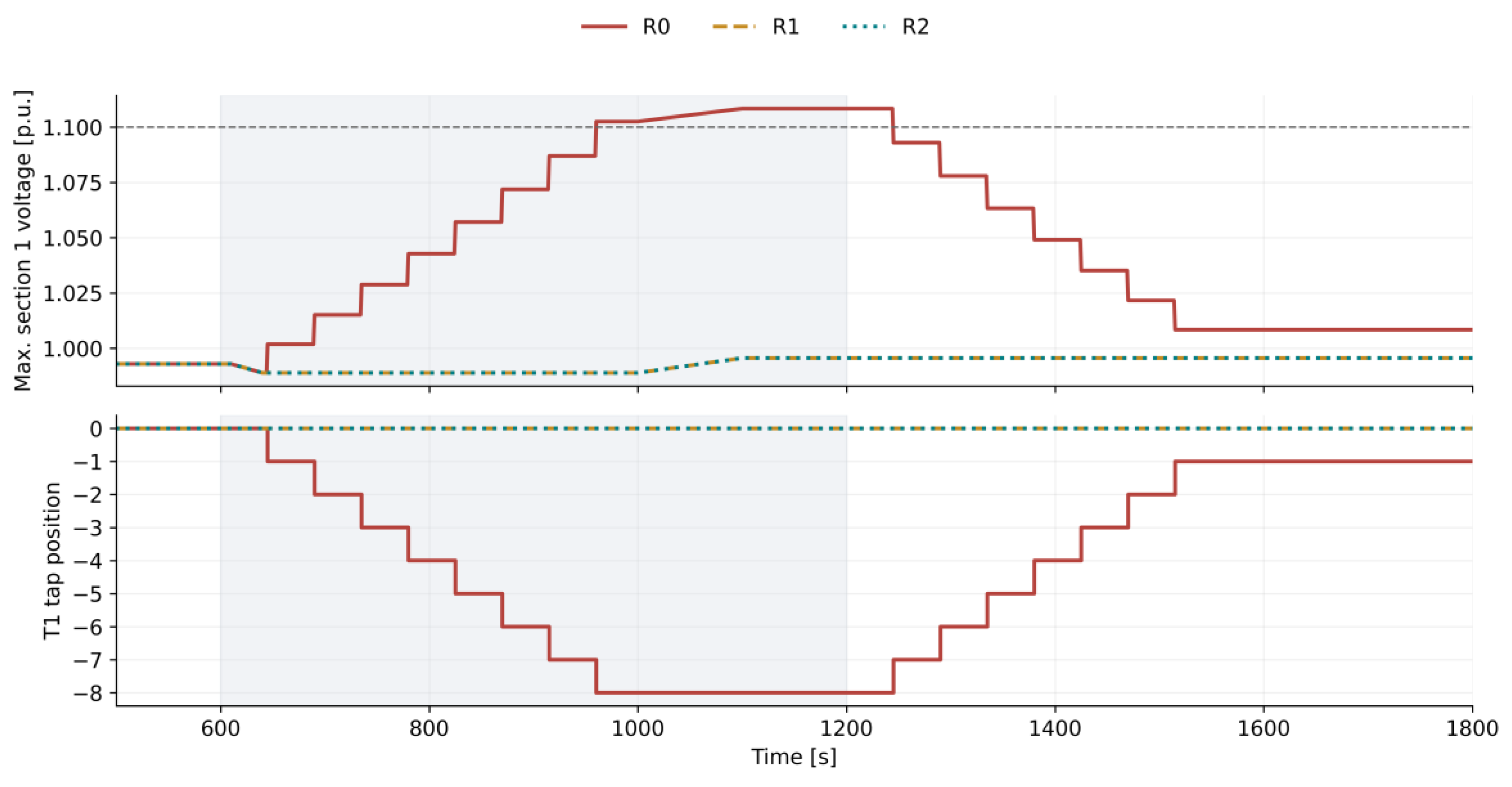
The largest single-trial JV was 13.3205 p.u.·s, obtained for a +0.10 p.u. setpoint change lasting 600 s at a load scaling factor of 0.6 with R0. Violations lasted 285 s and affected nine section 1 buses; T1 performed 15 tap changes. After incident termination, recovery to the adopted band took 45 s. The maximum integrated violation occurs in a different case from the voltage extremum, so both metrics are retained in the dataset.
3.2. Tap Changes and Detection Limitations
With FDI of +0.05 p.u., the basic controller receives an inflated measurement and lowers the actual MV voltage. R1 does not reject this measurement because it lies within the admissible range and carries a current timestamp. R2 detects the discrepancy between measurements, and the local backup channel maintains regulation using an independent signal. Figure 3 illustrates changes in voltage and tap position even without violation of the lower limit of 0.90 p.u.
Across the incident matrix, the total number of T1 tap changes per architecture decreases from 612 for R0 to 404 for R1 and 230 for R2. The 43.1% reduction compares R2 with R1 at the scenario frequencies specified in this matrix. It cannot be interpreted as a percentage increase in OLTC service life because the model excludes contact wear, commutation currents and maintenance effects. The total number of tap changes in the paired reference runs is 150 per architecture; thus, the additional counts are 462, 254 and 80 for R0, R1 and R2, respectively. Comparison with the reference distinguishes normal regulating operations from additional incident-induced operations.
An incident lasting 30 s may end before the 40 s controller delay elapses. Omitting this delay would overestimate the number of mechanical responses. Conversely, rejecting an unauthorized setpoint does not guarantee that concurrent FDI has no effect. During a combined incident, R1 may detect an unauthorized setpoint change while continuing to regulate using the falsified measurement.
3.3. Communication Loss Under Varying Supply Voltage
No voltage-band violations occurred in series D1, but centralized R0 and R1 held the tap position unchanged during WAN loss. R2 allowed the backup channel to take over regulation. The local loop retained regulation capability independently of remote-supervision availability. Results are summarized in Table 8.
Figure 4.
WAN loss over 600–1200 s and changing source voltage at a load scaling factor of 1.0. Centralized R2 and local R0 coincide with the reference; centralized R0 holds the tap position unchanged.
Figure 4.
WAN loss over 600–1200 s and changing source voltage at a load scaling factor of 1.0. Centralized R2 and local R0 coincide with the reference; centralized R0 holds the tap position unchanged.
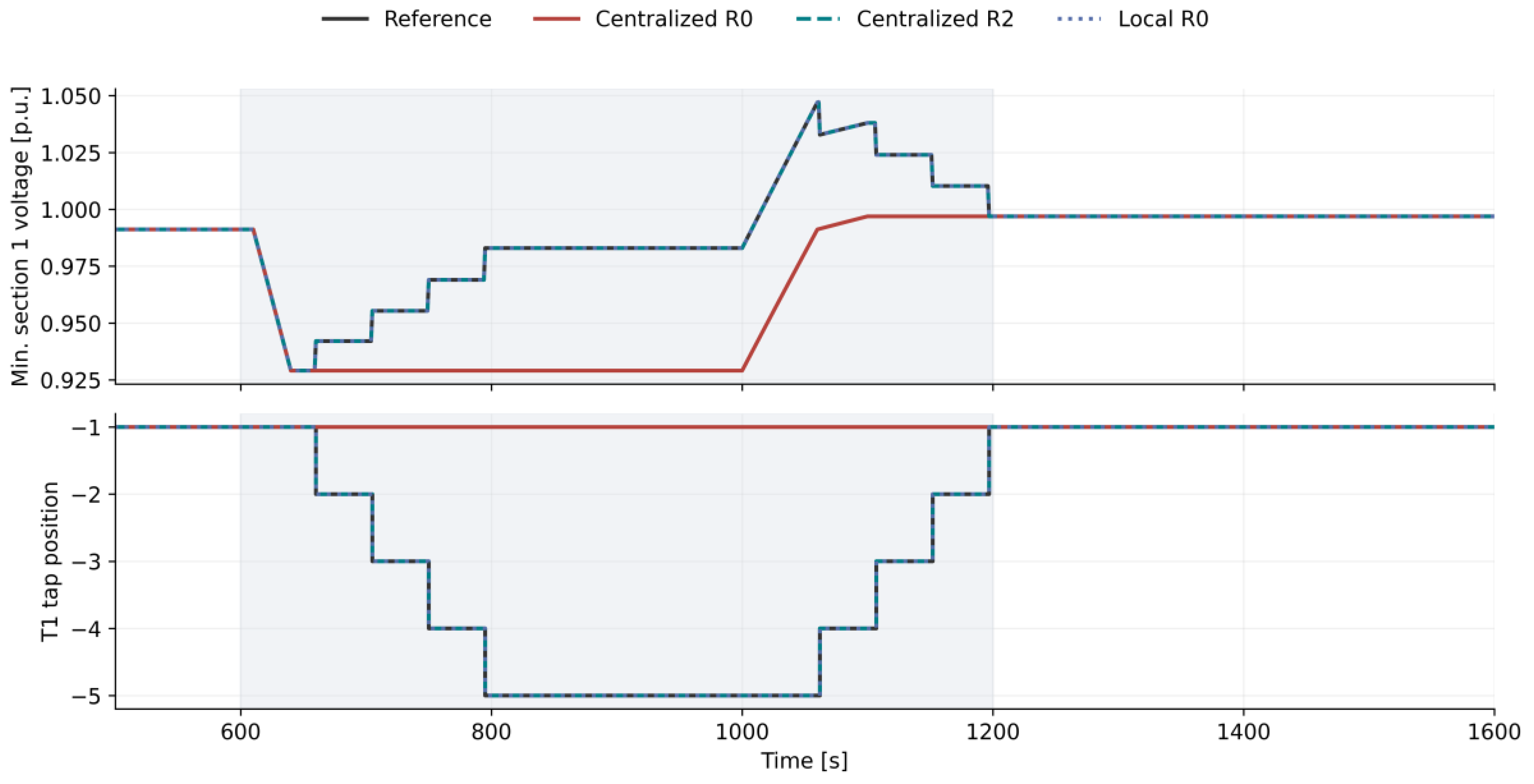
The larger number of tap changes in R2 than under command blocking reflects retained regulation in this case: eight operations match the reference response. For replay with refreshed timestamps, the measurement discrepancy increases only after supply conditions change, explaining detection after 21 s. The operation count alone is therefore insufficient to assess regulation performance and must be interpreted together with the voltage traces.
3.4. Random Variability and Sensitivity Analysis
Figure 5 presents the initial Monte Carlo results for 30 random realizations at a load scaling factor of 1.0. Comparisons use paired runs, following the procedure in Section 2.5.
For the −0.10 p.u. setpoint change with R0, the mean increase in JV was 1.1040 p.u.·s, with a 95% confidence interval of 0.8766–1.3314 p.u.·s; the median was 0.9999 p.u.·s. R1 and R2 produced zero increases in all 30 trials. R0 performed 16 additional tap changes in every trial, whereas R1 and R2 performed none. The zero-width interval for the tap-change count reflects absence of variability in the specified sample and does not demonstrate absence of uncertainty in an actual substation.
FDI of +0.05 p.u. caused eight additional tap changes in both R0 and R1 and none in R2. With consistent falsification of both channels, all three variants performed eight additional tap changes. In R0, FDI of +0.05 p.u. combined with a −0.05 p.u. setpoint change produced the same trace as a −0.10 p.u. setpoint change alone: both modifications create the same control error. They are neither independent evidence of effectiveness nor distinct physical responses.
Source-voltage sensitivity analysis covers 0.95 and 1.05 p.u. at three load levels. R2 takeover delays of 0, 30 and 120 s are examined separately. All 324 trials converged. In the source-voltage subset, R0 produced voltage-band violations in 12 of 30 incident cases per architecture; R1 and R2 produced none. The minimum R0 voltage was 0.88563 p.u. Absence of violations at the tested delays does not justify arbitrarily increasing the takeover time; the finding is limited to the selected disturbances and stiff-source assumptions.
3.5. Detection Threshold and Response Activation
Without noise, the R2 detector generated no alarm for errors of ±0.019 or ±0.020 p.u. For errors of ±0.021 p.u., an alarm was present from the first sample and backup regulation activated after 5 s. For an error ramping linearly from zero to ±0.05 p.u. over 600 s, the first alarm occurred after 241 s and takeover after 246 s. These delays follow from strict threshold exceedance and the 1 s time step: at 240 s the error equals the threshold. Absence of detection before threshold exceedance does not exclude an earlier effect on the controller. At a load scaling factor of 1.0, a +0.019 p.u. error produced ΔJE = 137.757 p.u.·s and two T1 tap changes without an alarm, while JV = 0. Randomized validation results are reported in Table 9.
Table 9 covers nine cyberattack scenarios among the 11 validation events, for the centralized architecture and 30 random realizations per case. The two sensor faults and normal operation are discussed in Section 3.7. Activation means at least one activation of backup regulation during the event. Identifiers correspond to the protocol scenarios. Table 10 supplements the comparison with paired R2 − R2B differences for all 11 events, including both faults.
With noise present, threshold exceedance depends on the realization of measurement disturbances. For FDI of +0.019 p.u., an alarm occurred in all 30 trials, but backup regulation activated in only one. For FDI of +0.021 p.u., both an alarm and takeover occurred in every trial. First threshold exceedance and an anomaly persisting continuously for 5 s are distinct events. An alarm therefore does not establish that the incident consequences have been mitigated.
In the separate threshold check, each of the three R2 thresholds produced 10/10 trials with an alarm and backup activation under FDI of +0.03 p.u., and 0/10 alarms during normal operation, in each architecture. This set does not establish an optimal threshold: the larger attack magnitude does not expose differences apparent only near the boundary. The previously adopted 0.02 p.u. threshold is retained.
A negative difference indicates a smaller increase in integrated voltage deviation with R2. BEN_BIAS_15 and BEN_BIAS_25 denote sensor faults with biases of +0.015 and +0.025 p.u.; other identifiers are defined in Table 9. Student’s t intervals are calculated from 30 individual differences; they are pointwise, without adjustment for multiple comparisons. A zero-width interval indicates identical differences within this sample. For TH_M19 and TH_P19, a zero median indicates that the mean effect arises from only part of the realizations. The interval for TH_P19 includes zero. S1 provides complete results for both architectures.
3.6. Communication Irregularities and the R2b–r2 Comparison
In the deterministic trial for the centralized architecture at a load scaling factor of 1.0, measurement-loss episodes lasting 2 s and recurring every 20 s produced neither an alarm nor an increase in integrated voltage deviation. For 5 s episodes, the first alarm occurred after 3 s, but R2 backup regulation did not activate. Repeated blocking caused by data-validation checks interrupted the 40 s controller timer. Consequently, T1 performed no tap changes and ΔJE reached 109.786 p.u.·s despite anomaly detection. A similar mechanism occurred with 2 s replay episodes. This limitation follows from the timing conditions for response activation.
For delays up to 8 s, R2 raised an alarm after 6 s, took over regulation after 18 s, and produced ΔJE = 1.449 p.u.·s with eight tap changes, compared with 109.786 p.u.·s and no tap changes for R2B. With 10 s mixed replay, the alarm occurred after 21 s and takeover after 26 s; ΔJE was 18.742 p.u.·s for R2 versus 109.786 p.u.·s for R2B. In the local loop, these remote-telemetry disturbances caused no difference from the reference.
In Table 11, both strategies initiate their response at the same instant, with identical detectors, thresholds and time delays. For FDI and WAN loss, backup regulation reproduces the reference trace, whereas blocking prevents the required tap changes. Once different responses are applied, system states may diverge; subsequent replay alarm sequences therefore need not be identical despite the shared detection algorithm.
Figure 6.
R2 under 5 s measurement-loss episodes every 20 s. The alarm interrupts regulation but does not persist long enough to activate backup regulation. Excerpt from a deterministic trial: centralized architecture, D1 and load scaling factor 1.0.
Figure 6.
R2 under 5 s measurement-loss episodes every 20 s. The alarm interrupts regulation but does not persist long enough to activate backup regulation. Excerpt from a deterministic trial: centralized architecture, D1 and load scaling factor 1.0.
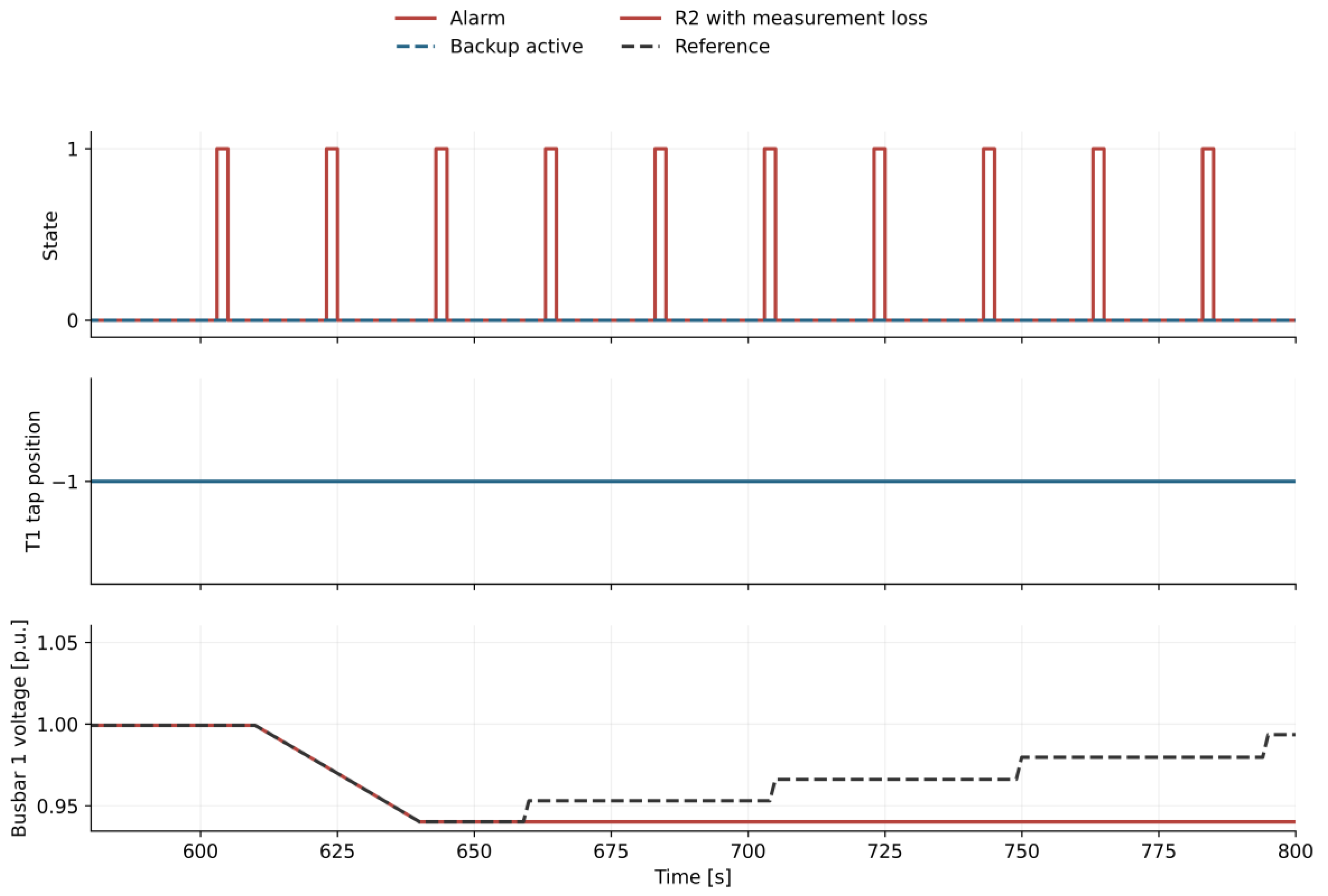
For 30 validation realizations, the mean paired difference ΔJE(R2) − ΔJE(R2B) was −91.946 p.u.·s for delays up to 8 s, with a 95% confidence interval of [−98.756, −85.136] p.u.·s. For 10 s mixed replay, it was −88.637 p.u.·s, with an interval of [−89.876, −87.398] p.u.·s. Negative values indicate a smaller increase in integrated voltage deviation with R2.
3.7. Normal Operation and Sensor Faults
No R2 alarm occurred in any of the 30 normal-operation trials for either architecture. For the centralized architecture, the 95% Wilson confidence interval is 0.0–11.4%. Absence of alarms in this sample therefore does not establish zero probability of occurrence. The result applies to the specified synthetic conditions and the noise standard deviation of 0.001 p.u.; it is not an estimate valid for arbitrary measurement-channel quality.
A modeled sensor bias of +0.015 p.u. triggered an alarm in 3 of 30 trials for the centralized architecture, while a bias of +0.025 p.u. did so in all 30 trials. These alarms correspond to injected measurement anomalies and are not classified as false alarms during normal operation. However, the detector cannot distinguish a sensor fault from FDI with an identical signal trace. In the series with the noise standard deviation increased to 0.003 p.u., a +0.015 p.u. sensor bias produced the first alarm after 12 s without backup activation. Thus, the distinction between instantaneous detection and satisfaction of the response timing condition also applies in the absence of an attack.
3.8. Partial Loss of Measurement Independence
Identical errors of +0.05/+0.05 p.u. and similar errors of +0.05/+0.045 p.u. remained undetected in the deterministic series. The inter-channel differences were 0 and 0.005 p.u., respectively. Under D1 at a load scaling factor of 1.0, both cases produced ΔJE = 243.258 p.u.·s, eight T1 tap changes and JV = 0 with R2. An incident can therefore evade detection without identical falsification of both measurements; an inter-channel difference below the threshold is sufficient.
When the second channel was compromised only after 60 or 180 s, R2 initially raised a correct alarm and activated backup regulation. Subsequently, consistent but erroneous data cleared the alarm and caused return to the primary channel after 60 s of apparent data validity. At a load scaling factor of 1.0, ΔJE was 171.539 and 140.912 p.u.·s, respectively, compared with zero when the second channel remained uncompromised. For a second-channel error of −0.01 p.u., the alarm persisted, but backup regulation used the biased measurement, giving ΔJE = 4.181 p.u.·s and 10 tap changes. An active alarm therefore does not ensure the quality of the data used for control.
In validation, consistent falsification of both channels was undetected in all 30 R2 trials for each architecture. This supports the use of independent sources of process information. An AI model relying exclusively on the same two falsified signals cannot be assumed to distinguish normal and attacked states.
3.9. Numerical Verification and Repeatability
Electrical verification covers 1350 operating points: both sections, all 25 tap positions, three source-voltage levels and nine load levels, including no load. Maximum residuals are 7.97 × 10⁻¹³ p.u. for impedance voltage-drop equations, 1.76 × 10⁻¹⁶ p.u. for bus current balances, 4.69 × 10⁻¹² MW for active power balance and 1.98 × 10⁻¹¹ Mvar for reactive power balance. The checks include cable capacitances and transformer losses. At 24 points, comparison with an independent solution of the P and Q equations using the admittance matrix yields a maximum voltage difference of 7.81 × 10⁻¹³ p.u. This confirms implementation consistency with Ohm’s and Kirchhoff’s laws within the adopted model; it does not replace validation against field measurements.
Table 12 presents time-step analysis for a −0.10 p.u. setpoint change lasting 600 s at a load scaling factor of 1.0 with R0. The difference in JV between the 1 and 0.5 s steps is approximately 0.031%; for the 2 s step it is approximately 7.76% relative to 0.5 s. These differences arise from discretization of event timing and integration. A 1 s step is used in the other analyses. This check concerns a single case and does not quantify time-discretization error across the entire matrix.
The 6990-trial protocol was executed three times under separate organizational result-storage profiles, yielding 20,970 simulation runs. Results were compared after excluding profile labels and storage paths while retaining physical metrics and trace hashes. Summary and trace hashes matched across all three executions. These repetitions constitute an automated computational repeatability check, not independent experimental replications by the individual authors. They do not increase the statistical sample size; summaries and between-strategy differences are calculated separately for each profile.
S1 contains 20,970 individual results, their configurations and trace hashes, and a report comparing the three profiles. Electrical, time-step and software-test reports are linked to the code and reproduction instructions. Additional checks do not increase the protocol trial count. Complete time-series arrays can be regenerated from the configurations; the program supports saving them in NPZ format.
Across the extended protocol, the maximum cable current was 303.994 A and the maximum reported transformer loading was 86.31%. These quantities were used to check consistency of the operating points analyzed. They are not outcomes of thermal, overload or short-circuit studies and do not establish permissible equipment operation in states outside the model.
4. Discussion
4.1. Interpretation and Relationship to the Literature
The results show the need to distinguish input-data validity, detection effectiveness and preservation of regulation after anomaly detection. In the main matrix, R1 and R2 achieved the same outcome under the criterion JV = 0 but differed in additional tap-change counts. Conversely, under varying supply voltage, reducing the operation count to zero degraded the voltage profile. Tap-change counts must therefore be interpreted relative to the need for regulation and the paired reference run.
The voltage effects of false data are consistent with mechanisms considered in studies of centralized control and tap changers [2,3,4,6]. The central comparative finding is the isolation of the post-detection response: with the detector unchanged, R2 could retain voltage regulation that R2B blocking could not provide. The approach uses the existing transformer regulation function and an independent measurement channel. Methods based on reactive power control, reconfiguration or distributed-resource control [5,6,7,8] have a different range of available control actions. Without a common test model and identical scenarios, these results cannot establish the superiority of one class of methods.
The communication-irregularity results reveal the importance of the relationship between anomaly duration, protection activation delay and OLTC controller delay. Brief alarms may repeatedly interrupt timing of a tap change without satisfying the condition for backup activation. This is a limitation of detector–controller interaction that the detection rate alone does not capture. Any modification of alarm-latching logic would require a separate study of its effects on false activations, regulation performance and safe return to the primary channel.
Backup-channel effectiveness remains conditional on the trustworthiness of its measurement, drive connection and setpoint. Similar errors in both sensors may remain below the discrepancy threshold, while delayed falsification of the second channel may create an apparent return to normal conditions. Likewise, the same measurement-error trace may arise from a fault or deliberate manipulation. Anomaly detection must therefore be distinguished from cause identification, and alarms must be interpreted cautiously as evidence of a cyberattack.
4.2. Limitations and Generalizability
The model excludes distributed generation, unbalance, short circuits, electromagnetic dynamics, tripping protection and actual communication-protocol implementations. Communication irregularities are represented as events at the controller input. The model scope does not support estimation of energy not supplied, OLTC service life or transient stability. Threshold checks and validation use disjoint generator seed sets but the same model family and synthetic disturbances. They therefore provide neither out-of-distribution validation nor validation against measurements from a real substation. The threshold series covers defined error magnitudes without an exhaustive analysis of adaptive attacks. Conclusions about resilience and regulation performance are limited to the scenarios examined.
The reported event proportions and reductions in tap changes depend on the design of the experimental matrix. They do not estimate operational incident risk. Confidence intervals across random realizations describe variability within the adopted perturbation model; they exclude uncertainty in model structure, actual equipment parameters and unknown attacker actions. Reproduction requires the code version, configurations, generator seeds and result data needed to recreate the tables and figures.
4.3. Future Research
The identified limitations motivate comparison of the threshold detector with model-based and sequential methods, followed by AI methods. Beyond the difference between two measurements, candidate inputs include electrical balance residuals, tap-position and command histories, P, Q and I measurements, communication metadata, and signal-quality and provenance information. The objective is to distinguish normal operating changes, sensor faults, communication degradation and data manipulation. Separability of these classes requires explicit assessment because identical observations may prevent unique identification of the cause.
Training, validation and test sets should be separated at the level of complete runs, and generalization should be assessed across distinct topologies and attack families. This reduces information leakage through neighboring samples from the same event. Evaluation should include detection rate, response time, alarms per hour of normal operation, changes in regulation performance, predictive uncertainty, and behavior under drift and out-of-distribution data. Resistance of AI methods to manipulation of input and training data should also be assessed. Studies [8,9,10] provide a basis for comparing machine-learning methods with rule-based and model-based detectors.
Figure 7 outlines the next research stages. Modeling and evaluation of deterministic protection strategies are to be followed by hardware-in-the-loop (HIL) validation using physical intelligent electronic devices (IEDs) and substation communications, and subsequently by evaluation using operational data. Platforms [12,13] provide reference approaches for this stage. Initial AI use should be restricted to supervision without automatic command issuance. Introducing AI into control requires a separate demonstration of benefit and verification of safe fallback to deterministic regulation. Setpoint limits, blocking and independent backup regulation should remain outside the exclusive control of the learned model. Progress to subsequent stages depends on establishing model adequacy; the present results do not establish readiness for deployment.
5. Conclusions
In the reference 110/15 kV substation, incidents in the OLTC control loop altered bus voltages and tap-change counts even when the inputs passed basic validity checks. In the main matrix, R1 and R2 prevented the 0.90–1.10 p.u. voltage-band violations observed in 9 of 225 R0 trials per architecture. R2 reduced the total tap-change count from 404 to 230 relative to R1, or by 43.1%. This result applies to the adopted matrix and does not quantify a change in OLTC service life.
Comparing R2B and R2 with the same detector demonstrated the benefit of retaining regulation under varying supply voltage. However, brief recurring anomalies could trigger alarms without backup activation, while similar errors in both measurement channels remained undetected. Local-loop autonomy limited the effects of remote communication loss but did not eliminate the effects of falsifying its measurement. Protection assessment should therefore combine voltage metrics, additional tap-change counts, and detection and response times. These results provide a basis for further research; establishing operational applicability requires hardware validation and comparison with measured data.
Supplementary Materials
The following supporting information can be downloaded at the website of this paper posted on Preprints.org. S1_GPZ_Code_Data_Verification.zip: GPZ CyberLab 2.1.0 source code, protocol and configurations, individual JSON/CSV and Excel results, statistical summaries, verification reports, and instructions and scripts for reproducing tables and figures.
Author Contributions
Conceptualization, methodology, software, validation, formal analysis, investigation, resources, writing—original draft preparation, visualization, supervision, project administration and funding acquisition, S.W.; data curation and writing—review and editing, S.W., T.S. and A.K. All authors have read and approved the manuscript and agreed to its submission.
Funding
This research was funded by the authors from their own resources and received no external funding. The article processing charge will be paid by the authors from their own resources.
Data Availability Statement
GPZ CyberLab 2.1.0 code, configurations and generator seeds, individual results from three protocol executions, Excel tables and reports are provided in S1. The instructions describe reproduction of traces and summaries; file integrity is documented by a SHA-256 manifest. The data are generated by simulations of the reference system.
Conflicts of Interest
The authors declare no conflicts of interest.
References
- Stouffer, K.; Pease, M.; Tang, C.; Zimmerman, T.; Pillitteri, V.; Lightman, S.; Hahn, A.; Saravia, S.; Sherule, A.; Thompson, M. Guide to Operational Technology (OT) Security; NIST Special Publication 800-82, Revision 3; National Institute of Standards and Technology: Gaithersburg, MD, USA, 2023. [Google Scholar] [CrossRef]
- Isozaki, Y.; Yoshizawa, S.; Fujimoto, Y.; Ishii, H.; Ono, I.; Onoda, T.; Hayashi, Y. Detection of Cyber Attacks Against Voltage Control in Distribution Power Grids With PVs. IEEE Trans. Smart Grid 2016, 7, 1824–1835. [Google Scholar] [CrossRef]
- AlMajali, A.; Alasali, F.; El-Naily, N.; Abuashour, M.I.; Abu Ghalyon, S. Impact of Cyberphysical Attacks on Load Tap Changers and Distribution System Voltage Stability. IET Smart Grid 2026, 9, e70076. [Google Scholar] [CrossRef]
- Bragatto, T.; Bucarelli, M.A.; Bucarelli, M.S.; Carere, F.; Geri, A.; Maccioni, M. False Data Injection Impact on High RES Power Systems with Centralized Voltage Regulation Architecture. Sensors 2023, 23, 2557. [Google Scholar] [CrossRef] [PubMed]
- Naderi, E.; Asrari, A. Cyber-Physical Distribution Systems Resilience Against Cyberattacks via a Remediation Framework Based on Static VAR Compensators (SVCs). IEEE Access 2024, 12, 119633–119646. [Google Scholar] [CrossRef]
- Naderi, E.; Asrari, A. A Remediation Framework Against False Data Injection Cyberattacks Targeting ULTC Transformers to Avoid Voltage Collapse in Smart Distribution Networks. IEEE Trans. Ind. Appl. 2025, 61, 5148–5160. [Google Scholar] [CrossRef]
- Naderi, E.; Asrari, A. Mitigating Voltage Violations in Smart City Microgrids Under Coordinated False Data Injection Cyberattacks: Simulation and Experimental Insights. Smart Cities 2025, 8, 20. [Google Scholar] [CrossRef]
- Selim, A.; Zhao, J.; Ding, F.; Miao, F.; Park, S.-Y. Deep Reinforcement Learning for Distribution System Cyber Attack Defense with DERs. In Proceedings of the 2023 IEEE Power & Energy Society Innovative Smart Grid Technologies Conference (ISGT), Washington, DC, USA, 16–19 January 2023; pp. 1–5. [Google Scholar] [CrossRef]
- Zhang, F. Event–Triggered Neural Network Voltage Control for Distribution Networks under Actuator Attacks based on Observers. Int. J. Appl. Math. Comput. Sci. 2026, 36, 81–90. [Google Scholar] [CrossRef]
- Ang, T.-Z.; Salem, M.; Kamarol, M.; Abdolrasol, M.G.M.; Ustun, T.S.; Cali, U. Cyber-Resilient Control Based on Soft Reinforcement Learning for Inverter-Based PV/FC Systems: Real-Time Implementation and Validation. Energy Rep. 2026, 15, 109241. [Google Scholar] [CrossRef]
- Li, Z.; Wang, M.; Yan, Y.; Qi, D.; Xu, Z.; Zhang, J.; Wang, Z. Tube Model Predictive Control Based Cyber-Attack-Resilient Optimal Voltage Control Strategy in Wind Farms. CSEE J. Power Energy Syst. 2024, 10, 530–538. [Google Scholar] [CrossRef]
- Vallam Kondu, S.C.; Ravikumar, G.; Mohan, S.N. CPS-DERMS: Cyber-Physical Security and Impact Analysis of DERMS Against MITM Attacks. In Proceedings of the 2025 IEEE Green Technologies Conference (GreenTech), Wichita, KS, USA, 26–28 March 2025; pp. 1–5. [Google Scholar] [CrossRef]
- Cibin, N.; Kabbara, N.; Presekal, A.; Semertzis, I.; Rajkumar, V.S.; Goyel, H.; Palensky, P.; Ştefanov, A. Cyber–Physical Power System Dataset for Cyber Security of Digital Substations. IEEE Access 2026, 14, 83420–83433. [Google Scholar] [CrossRef]
- Energa-Operator. Technical Standards at ENERGA-OPERATOR SA (in Polish); Version 35. 29 September 2025. Available online: https://cdn-netpr.pl/file/mediakit/2896260/0/20250929_st_standardy_techniczne_w_eop_sa_w35.pdf (accessed on 16 September 2026).
- Fabryka Transformatorów w Żychlinie. Power Transformers: TORc 25000/115F. Available online: https://www.ftz.pl/en/transformatory-mocy.php (accessed on 16 September 2026).
- Kable, T.E.L.E.-F.O.N.I.K.A. Clean Energy Cables; NA2XSY 12/20 kV, 1×240RMC/50. pp. 28–30. Available online: https://www.tele-fonika.com/storage/file/core_files/2025/3/5/e4bd6d432036f1cb3810255a0031d7e6/Clean%20Energy%20Cables.pdf (accessed on 16 September 2026).
- Maschinenfabrik Reinhausen. TAPCON 260: Operating Instructions 1801002/04 EN; Three-Winding Transformer; 2014; Section 7.4. pp. 65–70. Available online: https://www.reinhausen.com/fileadmin/downloadcenter/products/voltage_regulators/discontinued_products/tapcon_260/ba/three-winding_transformer/ba1801002_04_en_tapcon260_dreiwickler.pdf (accessed on 16 September 2026).
Figure 3.
FDI of +0.05 p.u. for 600 s at a load scaling factor of 1.0. R0 and R1 traces coincide; R2 limits unwanted tap changes.
Figure 3.
FDI of +0.05 p.u. for 600 s at a load scaling factor of 1.0. R0 and R1 traces coincide; R2 limits unwanted tap changes.
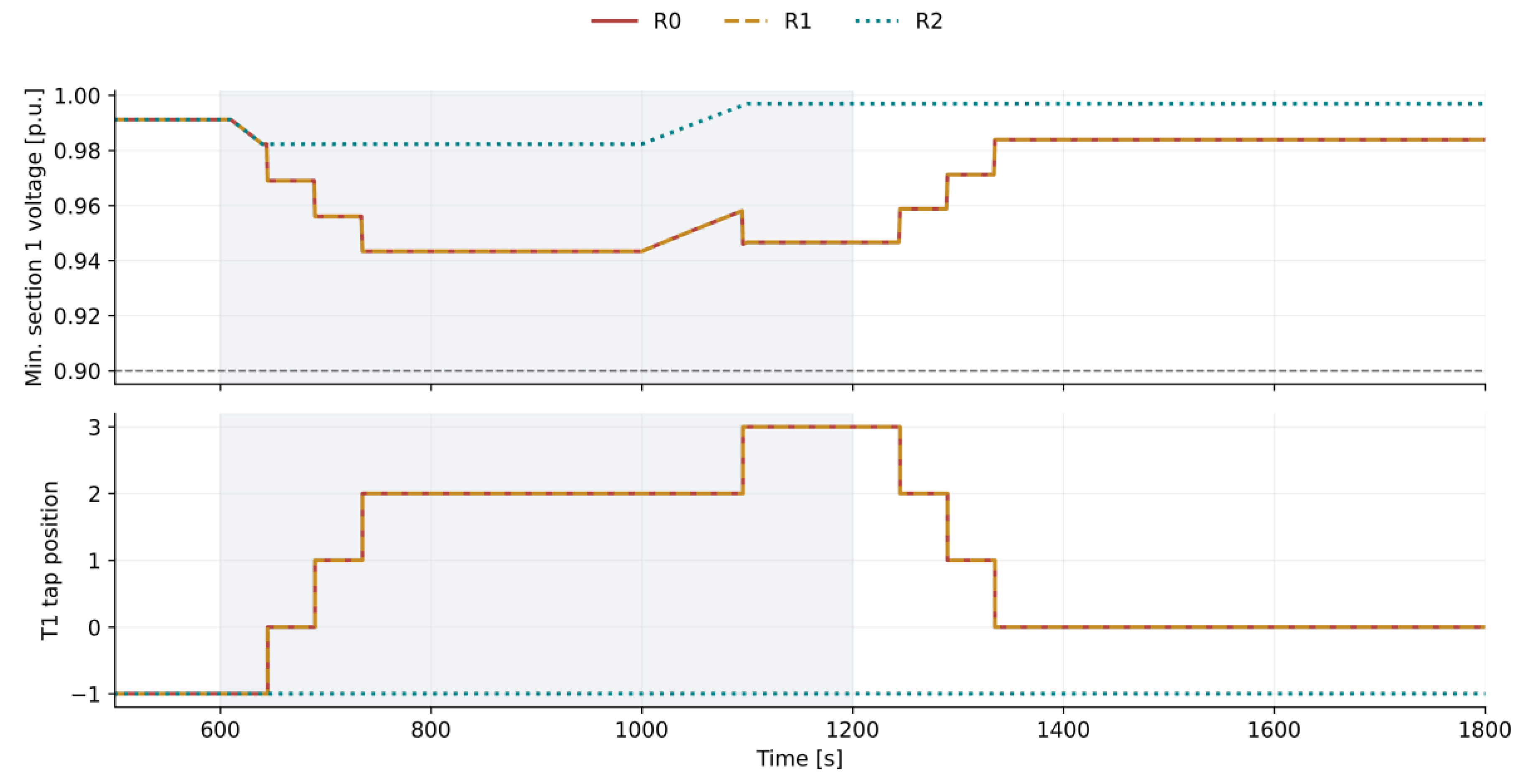
Figure 5.
Monte Carlo analysis for the centralized architecture and 30 random realizations. Left: ΔJV for a −0.10 p.u. setpoint change and the 95% confidence interval for the mean. Right: mean additional T1 tap-change counts.
Figure 5.
Monte Carlo analysis for the centralized architecture and 30 random realizations. Left: ΔJV for a −0.10 p.u. setpoint change and the 95% confidence interval for the mean. Right: mean additional T1 tap-change counts.
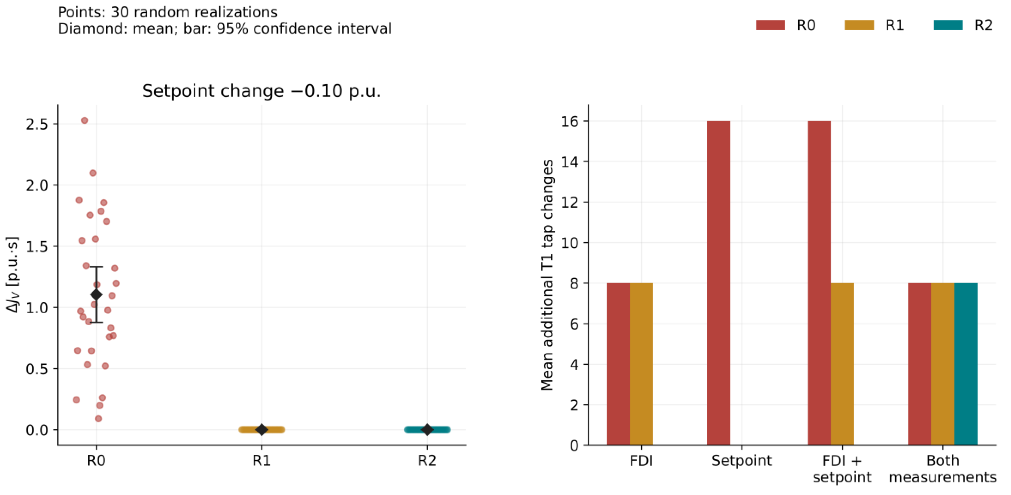
Figure 7.
Research program on cyber-physical resilience of power systems. Shaded boxes indicate the scope of this work; dashed boxes indicate future stages. HIL: hardware-in-the-loop; IED: intelligent electronic device.
Figure 7.
Research program on cyber-physical resilience of power systems. Shaded boxes indicate the scope of this work; dashed boxes indicate future stages. HIL: hardware-in-the-loop; IED: intelligent electronic device.
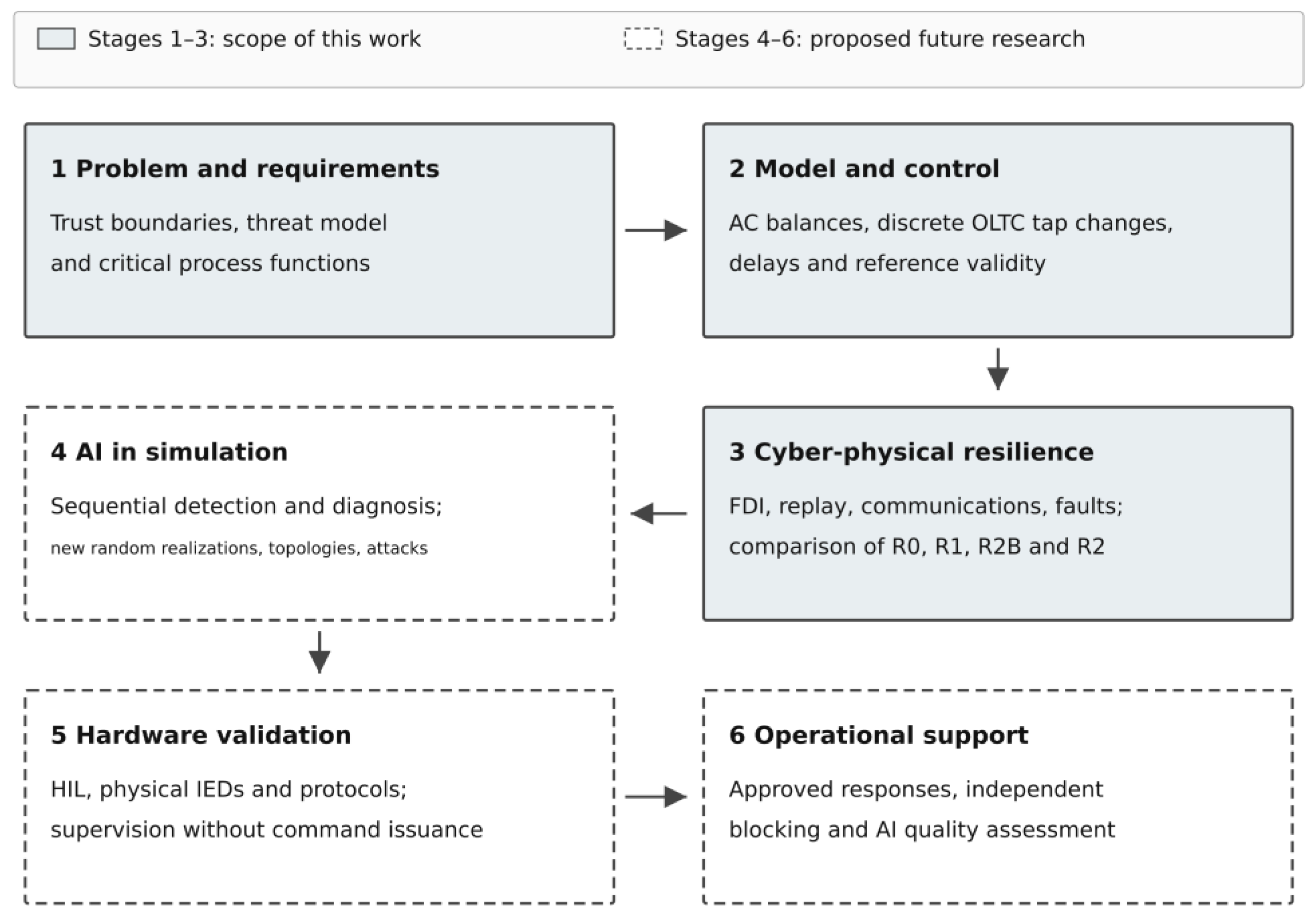

Table 1.
Scope of related studies and their relationship to the present work.
| Publication | Scope and verification method | Relationship to this work |
| Bragatto et al. 2023 [4] | FDI targeting centralized voltage regulation; IEEE 118-bus system with high RES penetration. | Same mechanism linking false data to regulation. This work includes a discrete OLTC loop and backup regulation. |
| Selim et al. 2023 [8] | Soft actor–critic (SAC) reinforcement learning; control of distributed resources and loads; modified IEEE 33-bus system. | Attack mitigation while retaining control capability. R2 is a rule-based baseline for future AI methods. |
| Li et al. 2024 [11] | Robust wind-farm voltage control using cascaded tube model predictive control (MPC); IEEE 14- and 118-bus systems. | Shared focus on physical consequences. Differences in models and actuators limit direct result comparisons. |
| Naderi and Asrari 2024 [5] | Static VAR compensators (SVCs), reactive power control and reconfiguration; 33-, 95- and 136-bus systems. | Mitigation using network resources. This work evaluates backup OLTC regulation without reconfiguration or additional sources. |
| Naderi and Asrari 2025 [6] | FDI targeting under-load tap changers (ULTCs); reconfiguration and load management; 33- and 136-bus systems. | Same problem of transformer-ratio manipulation. This work compares R2B and R2 with the same detector to assess the consequences of blocking regulation. |
| Naderi and Asrari 2025 [7] | Coordinated FDI and voltage violations in microgrids; simulation and experimental investigation. | Reference for combined incidents. This work distinguishes simultaneous and delayed falsification of the second measurement channel. |
| Vallam Kondu et al. 2025 [12] | Man-in-the-middle (MITM) attacks on DERMS; OPAL-RT, ns-3 and Python control; HIL testing. | Related impact metrics: voltages and additional tap changes. HIL testing extends validation beyond software simulation. |
| AlMajali et al. 2026 [3] | Attacks on load tap changers (LTCs); RTDS and a distribution system with PV. | Same mechanism of voltage changes caused by ratio manipulation. Perturbation models and network parameters differ from the loop examined here. |
| Zhang 2026 [9] | Adaptive neural controller, observers and event triggering; stability conditions and simulations. | Reference for AI-based control studies. These results do not establish performance in the substation model examined here. |
| Ang et al. 2026 [10] | Photovoltaic/fuel-cell (PV/FC) control using soft reinforcement learning; real-time implementation and validation. | Example of progression from a model to implementation. Different time scales and actuators limit comparison with OLTC control. |
| Cibin et al. 2026 [13] | Dataset combining RTDS and physical/virtual IEDs; voltages, currents, IEC 61850 traffic and device resource utilization. | Reference for data selection in future detector validation. The present model excludes actual protocol traffic. |
Table 2.
Reference-model parameters and data sources.
| Component | Model values | Source |
| Transformers T1 and T2 | 25 MVA; 115/15.75 kV; uk = 11%; YNd11 | FT Żychlin TORc 25000/115F [15] |
| Losses and taps | Pk = 155 kW; P0 = 12 kW; ±12 steps of 1.25% |
Manufacturer data [15] |
| MV cable | NA2XSY 12/20 kV 1×240RMC/50 | TELE-FONIKA Kable [16] |
| Cable parameters | R90 = 0.161 Ω/km; X = 0.108 Ω/km; C = 0.27 μF/km | Trefoil arrangement [16] |
| Load powers and section lengths | 1.2 / 1.1 / 0.9 MW; 1 / 1.5 / 2 km; cos φ = 0.95 | Study assumptions |
| Feeder participation factors | 0.85 / 1 / 1.15 and 0.9 / 1 / 1.1 | Study assumptions |
Table 3.
Intervals with constant load-multiplier values.
| Time [s] | 0–610 | 640–1000 | 1100–1800 | 2000–2600 | 2800–3600 |
| Multiplier | 1 | 1.3 | 0.8 | 1.15 | 1.0 |
Table 4.
Protection strategies and response logic.
| Strategy | Implemented logic |
| R0 | Basic regulation. The last measurement is held after telemetry loss. Loss of the command channel prevents new tap-change commands. |
| R1 | R0 plus checks of the measurement range (0.7–1.3 p.u.), data age (3 s), message ordering and setpoint range (0.97–1.03 p.u.). Invalid measurements block new commands; inadmissible setpoints are rejected. A watchdog detects absence of the communication heartbeat. |
| R2 | R1 plus comparison of the primary and independent local measurements, with a discrepancy threshold of 0.02 p.u. After an uninterrupted anomaly lasting 5 s, the backup channel takes over regulation. Return to the primary channel follows 60 s of data classified as valid. |
| R2B | Same detector as R2, with a 5 s activation delay and return after 60 s of data classified as valid. New commands are blocked instead of using backup regulation. Operations initiated before blocking are completed, as in R2. Included in the extended series. |
Table 5.
Incident types and imposed perturbations.
| Incident | Parameters varied in the experiment |
| Measurement falsification | Additive errors of ±0.01 / ±0.03 / ±0.05 p.u. at the T1 controller input. |
| Unauthorized setpoint change | Setpoint changes of ±0.02 / ±0.05 / ±0.10 p.u. |
| Replay attack | Cyclic replay of 30, 120 or 300 s of pre-attack history, retaining or refreshing the timestamp and sequence number. |
| Communication loss | Loss of telemetry, the command channel or WAN connectivity; queued commands are not executed when the channel is restored. |
Table 6.
Scope and size of the simulation series.
| Series | Design or scope | Trials |
| Main | 76 × 3 load levels × 2 architectures × R0/R1/R2 | 1368 |
| Initial Monte Carlo | 30 realizations × 6 cases × 2 architectures × 3 strategies | 1080 |
| Initial sensitivity | Source voltage and takeover delay | 324 |
| Source D1 | 5 cases × 3 load levels × 2 × 3 | 90 |
| Detection boundary | 9 cases × 3 load levels × 2 × 4 | 216 |
| Communication | 7 cases × 3 load levels × 2 × 4 | 168 |
| Non-attack events | 5 cases × 3 operating conditions × 2 × 4 | 120 |
| Detector and backup | 4 cases × 3 load levels × 2 × 4 | 96 |
| Channel independence | 7 cases × 3 load levels × 2 × 4 | 168 |
| Threshold check | 10 realizations × 3 thresholds × 2 cases × 2 architectures × 4 strategies | 480 |
| Extension validation | 30 new realizations × 12 cases × 2 architectures × 4 strategies | 2880 |
| Total | 2862 initial trials + 4128 new trials | 6990 |
| Three protocol executions | 3 repetitions of 6990 trials | 20,970 |
Table 7.
Main-matrix results for 225 incident trials per variant.
| Architecture | Strategy | Violation trials / 225 | ΣJV [p.u.·s] | T1 tap changes | Alarm trials / 225 |
| Centralized | R0 | 9 | 41.6103 | 612 | 0 |
| Centralized | R1 | 0 | 0.0000 | 404 | 108 |
| Centralized | R2 | 0 | 0.0000 | 230 | 153 |
| Local | R0 | 9 | 41.6103 | 612 | 0 |
| Local | R1 | 0 | 0.0000 | 404 | 72 |
| Local | R2 | 0 | 0.0000 | 230 | 117 |
Table 8.
Series D1 results at a load scaling factor of 1.0.
| Variant at load scaling factor 1.0 | ΔJE [p.u.·s] | T1 tap changes | Detection time [s] |
| Centralized R0, WAN loss | 109.786 | 0 | Not detected |
| Centralized R1, WAN loss | 109.786 | 0 | 3 |
| Centralized R2, WAN loss | 0.000 | 8 | 3 |
| Local R0, WAN loss | 0.000 | 8 | Not applicable to local loop |
| Centralized R2, replay with refreshed timestamps | 12.030 | 8 | 21 |
Table 9.
R2 and R2B results for nine cyberattack scenarios in validation of the centralized architecture.
Table 9.
R2 and R2B results for nine cyberattack scenarios in validation of the centralized architecture.
| Scenario and identifier | R2 alarm trials | R2 activation trials | Mean ΔJE R2 [p.u.·s] | Mean ΔJE R2B [p.u.·s] |
| FDI −0.019 p.u. TH_M19 |
30/30 | 6/30 | 28.918 | 46.507 |
| FDI +0.019 p.u. TH_P19 |
30/30 | 1/30 | 61.683 | 63.875 |
| FDI +0.021 p.u. TH_P21 |
30/30 | 30/30 | 3.156 | 104.746 |
| FDI ramping to +0.05 p.u. TH_RAMP_P |
30/30 | 30/30 | 13.110 | 95.504 |
| 5 s measurement loss every 20 s COM_BURST_5 |
30/30 | 0/30 | 103.572 | 103.572 |
| Packet delays up to 8 s COM_JITTER_8 |
30/30 | 30/30 | 12.989 | 104.935 |
| 10 s replay every 20 s COM_MIX_10 |
30/30 | 30/30 | 16.641 | 105.278 |
| Consistent FDI of +0.05 p.u. in both channels IND_EQUAL |
0/30 | 0/30 | 231.202 | 231.202 |
| FDI +0.05 p.u.; second channel +0.045 p.u. after 180 s IND_CLOSE_DELAY180 |
30/30 | 30/30 | 143.973 | 227.020 |
Table 10.
Paired differences ΔJE(R2) − ΔJE(R2B) for the centralized architecture; n = 30 pairs per event.
Table 10.
Paired differences ΔJE(R2) − ΔJE(R2B) for the centralized architecture; n = 30 pairs per event.
| Scenario |
Mean [p.u.·s] |
95% confidence interval for the mean [p.u.·s] |
Median [p.u.·s] |
| TH_M19 | −17.589 | [−31.639, −3.539] | 0.000 |
| TH_P19 | −2.192 | [−6.675, 2.291] | 0.000 |
| TH_P21 | −101.590 | [−105.446, −97.734] | −107.863 |
| TH_RAMP_P | −82.394 | [−89.127, −75.661] | −81.591 |
| COM_BURST_5 | 0.000 | [0.000, 0.000] | 0.000 |
| COM_JITTER_8 | −91.946 | [−98.756, −85.136] | −92.392 |
| COM_MIX_10 | −88.637 | [−89.876, −87.398] | −88.769 |
| IND_EQUAL | 0.000 | [0.000, 0.000] | 0.000 |
| IND_CLOSE_DELAY180 | −83.048 | [−88.705, −77.390] | −80.180 |
| BEN_BIAS_15 | 0.000 | [0.000, 0.000] | 0.000 |
| BEN_BIAS_25 | −102.186 | [−106.100, −98.271] | −109.052 |
Table 11.
Comparison of R2B and R2 responses under D1 at a load scaling factor of 1.0.
| Incident under D1 | Detection time [s] | Activation time [s] | ΔJE R2B [p.u.·s] | ΔJE R2 [p.u.·s] | Tap changes R2B / R2 |
| FDI +0.05 | 0 | 5 | 109.786 | 0.000 | 0 / 8 |
| WAN loss | 3 | 8 | 109.786 | 0.000 | 0 / 8 |
| Replay with refreshed timestamps | 21 | 26 | 109.786 | 12.030 | 0 / 8 |
Table 12.
Effect of the time step on a selected scenario.
| Time step [s] | JV [p.u.·s] | Minimum voltage [p.u.] | T1 tap changes |
| 0.5 | 1.207761 | 0.895493 | 16 |
| 1.0 | 1.207390 | 0.895493 | 16 |
| 2.0 | 1.114055 | 0.895493 | 16 |
Disclaimer/Publisher’s Note: The statements, opinions and data contained in all publications are solely those of the individual author(s) and contributor(s) and not of MDPI and/or the editor(s). MDPI and/or the editor(s) disclaim responsibility for any injury to people or property resulting from any ideas, methods, instructions or products referred to in the content. |
© 2026 by the authors. Licensee MDPI, Basel, Switzerland. This article is an open access article distributed under the terms and conditions of the Creative Commons Attribution (CC BY) license (http://creativecommons.org/licenses/by/4.0/).
Copyright: This open access article is published under a Creative Commons CC BY 4.0 license, which permit the free download, distribution, and reuse, provided that the author and preprint are cited in any reuse.