

Submitted:
26 September 2026
Posted:
28 September 2026
You are already at the latest version
Abstract
Extreme Gaussian tail probabilities arise in a wide range of statistical applications, including large--scale hypothesis testing, meta--analysis, and risk assessment. Although the normal distribution is analytically well understood, reliable numerical evaluation of the tail probability \[ 1-\Phi(Z) \] becomes challenging for large values of Z, due to the combined effects of numerical underflow, truncation of the infinite integration domain, and discretization error in numerical integration. In this work, we present a theoretically grounded framework for evaluating extreme Gaussian tail probabilities under standard double–precision arithmetic. Rather than introducing a new closed–form approximation, we reformulate the problem explicitly as a controlled numerical integration task and decompose the total numerical error into three independent components: underflow, truncation error, and numerical integration error. Central to this formulation are explicit analytical lower and upper bounds, F(Z) and G(Z), which satisfy \[ F(Z) \le 1-\Phi(Z) \le G(Z) \] and provide a rigorous enclosure of the true tail probability. Within this framework, numerical underflow is avoided by scale separation and logarithmic representations, truncation error is controlled by selecting a finite integration range based on the analytical bounds, and numerical integration error is regulated through standard quadrature error estimates. Numerical experiments show that, as \(Z\) increases, the effective integration range shrinks and the required subdivision number remains moderate, explaining the empirical robustness of Gaussian tail evaluations observed in practice. The proposed formulation does not aim to compete with existing highly optimized implementations based on minimax rational approximations. Instead, it provides a transparent theoretical interpretation of why such implementations remain stable and accurate even in extreme regimes. By explicitly connecting classical analytical bounds with numerical error control, this work offers a principled perspective on Gaussian tail evaluation and clarifies the structure underlying long--standing numerical practices.
Keywords:
normal distribution
; tail probabilities
; numerical integration
; Simpson method
1. Introduction
Accurate evaluation of Gaussian tail probabilities is a classical problem in statistics and numerical analysis. Quantities of the form
arise ubiquitously in statistical inference, hypothesis testing, extreme–value analysis, and many applied settings. From a numerical perspective, this problem is nontrivial, since the integrand decays rapidly and the target probability may fall far below machine precision for moderately large values of Z.
Highly optimized numerical implementations of the normal distribution function have therefore been developed and refined over several decades. A particularly influential approach is based on rational Chebyshev (minimax) approximations to the error function, as pioneered by Cody [1]. These approximations form the foundation of many modern software implementations, including the widely used pnorm function in the R statistical computing environment. Such methods achieve remarkable accuracy in double–precision arithmetic by carefully minimizing the worst–case approximation error over different regions of the real line.
Despite their numerical success, these implementations are largely opaque from a theoretical point of view. The interplay between underflow avoidance, truncation of the infinite integration domain, and numerical quadrature error is typically hidden within carefully tuned rational approximations. As a result, it is often difficult to relate empirical numerical robustness to classical analytical results, such as Mills–type bounds or other theoretical estimates of Gaussian tail behavior.
In this work, we revisit the computation of Gaussian tail probabilities from a complementary perspective. Rather than constructing a single global approximation, we formulate the problem explicitly as a controlled numerical integration task. Our approach decomposes the total numerical error into three distinct components: (i) underflow, addressed through appropriate scaling and log–domain representations; (ii) truncation error, controlled by selecting an integration domain that guarantees a prescribed bound on the neglected tail contribution; and (iii) numerical integration error, regulated by choosing the number of subintervals in accordance with error estimates for the quadrature scheme.
This explicit separation of error sources provides a transparent framework in which classical analytical bounds naturally emerge. In particular, well–known inequalities for Gaussian tails, such as those related to Mills’ ratio, arise directly as rigorous upper and lower bounds for the truncated integral. Within this framework, earlier empirical observations regarding the stability of numerical Gaussian tail evaluations can be understood and justified theoretically, rather than treated as purely algorithmic artifacts.
Importantly, the goal of the present work is not to compete with existing minimax–based implementations, which are highly optimized for floating–point performance. Instead, our contribution lies in providing a theoretically interpretable formulation that explains why such implementations are effective, clarifies the roles played by different error sources, and offers a principled basis for accuracy control. In this sense, the present analysis may be viewed as a theoretical underpinning of numerical techniques that have long been known to perform well in practice.
2. Methods
2.1. Problem Formulation
We consider the Gaussian tail probability
For large Z, direct numerical evaluation of this integral poses several challenges: the integrand rapidly underflows in floating–point arithmetic, the infinite integration domain must be truncated, and numerical quadrature errors must be controlled. These bounds are closely related to classical Mills-type inequalities for Gaussian tails and were also examined in our previous study from a geometric and numerical perspective [2]. In this section, we present a framework that explicitly decomposes these error sources and provides principled control over each component.
2.2. Analytical Bounds: The Backbone of the Method
A key role in our formulation is played by classical bounds on Gaussian tails. For , define the functions
It is well known that these functions satisfy the inequality
which follows from standard integration–by–parts arguments and properties of the Gaussian density. These bounds provide a rigorous enclosure of the true tail probability and serve as the theoretical backbone of our method. All subsequent algorithmic components are constructed so as to be consistent with this enclosure.
2.3. Control of Numerical Underflow
The Gaussian density decays super–exponentially as x increases, and thus direct evaluation of may underflow long before the integral itself becomes numerically negligible. To avoid this problem, we evaluate all quantities in a scaled or logarithmic form. Specifically, we represent the integrand as
and factor out the dominant exponential term . This scaling ensures that numerical underflow is avoided even for very large values of Z, while preserving the relative structure of the integral.
2.4. Control of Truncation Error via the Integration Range
The infinite integration domain must be replaced by a finite interval . The truncation error is defined by
Using the upper bound (4), we obtain
Hence can be chosen explicitly so that falls below a prescribed tolerance. This step decouples the control of truncation error from numerical integration error and provides a theoretically justified stopping criterion.
2.5. Control of Quadrature Error
After the infinite integration domain has been truncated to a finite interval, the remaining integral must be evaluated numerically. This introduces a third source of error, which is distinct from the truncation error discussed above. Whereas the truncation error arises from replacing the infinite interval by a finite one, the quadrature error arises from approximating the integral over that finite interval by a numerical integration rule.
In this study, we use the composite Simpson’s rule. Let the truncated integration interval be denoted by , where r is determined from the truncation criterion described in SubSection 2.4. Dividing this interval into N subintervals, the error of the composite Simpson’s rule can be bounded in terms of the fourth derivative of the integrand. For the standard normal density , the error satisfies
Since
the required number of subdivisions can be determined from Z, the integration range r, and a prescribed error tolerance . Here, the polynomial is the fourth probabilists’ Hermite polynomial. Specifically, it is sufficient to choose N such that
Thus, control of the quadrature error is reduced to selecting a sufficiently large value of N for the finite integration interval. This separates the error introduced by numerical integration from the truncation error and makes it possible to control the two sources of error independently.
3. Related Work
The numerical evaluation of the Gaussian distribution function and its tail has been studied extensively over the past several decades. Classical approaches to the numerical evaluation of special functions for digital computation were described by Hastings [4]. For the complementary error function, Shepherd and Laframboise [?] developed a Chebyshev approximation for a scaled form of . A particularly influential contribution was made by Cody [1], who developed rational Chebyshev (minimax) approximations for the error function.
By optimizing the worst–case approximation error over carefully chosen regions of the real line, Cody’s approach provides highly accurate function evaluations in floating–point arithmetic. These approximations form the foundation of many modern numerical libraries.
The implementation of the normal distribution function in the R statistical computing environment, pnorm, is a prominent example of this lineage. The R implementation combines Cody’s rational approximations with additional refinements, including explicit support for upper tails and logarithmic probability representations. In particular, the option log.p=TRUE enables stable evaluation of extremely small tail probabilities by operating directly in the logarithmic domain, thereby avoiding both underflow and catastrophic cancellation. As a result, pnorm exhibits remarkable numerical robustness even for very large values of Z.
In the Python ecosystem, Gaussian tail probabilities are implemented through several interfaces, including functions based on the complementary error function in the standard library and higher–level routines provided by packages such as SciPy. While these implementations are similarly rooted in classical approximation theory, their algorithmic structure and numerical guarantees are less uniform, reflecting the decentralized development of numerical functionality in the Python ecosystem
4. Numerical Experiments
In this section, we illustrate the behavior of the proposed framework through numerical experiments. All computations were carried out in double precision, and the results are presented in the logarithmic domain when appropriate. Rather than focusing on raw numerical values, our aim is to demonstrate how the different error components described in Section 2 behave as functions of Z.
4.1. Behavior of the Integration Constant
We first examine the quantity , which appears in the error bound for Simpson’s rule and reflects the contribution of higher–order derivatives of the integrand. Figure 1 shows as a function of Z. As predicted by the analytical discussion, increases with Z, reflecting the growing curvature of the Gaussian density in the tail region. This behavior alone would suggest an increasing numerical difficulty; however, as shown below, this effect is counterbalanced by the shrinking integration domain.
4.2. Integration Range and Truncation Error
Next, we consider the truncation of the infinite integration domain. Figure 2 displays the chosen integration range as a function of Z, determined so as to control the truncation error using the analytical upper bound . As Z increases, the required integration range decreases approximately as , in agreement with the classical asymptotic behavior of Gaussian tails. This shrinking of the effective domain plays a crucial role in maintaining numerical tractability in the large–Z regime.
4.3. Subdivision Number and Numerical Integration Error
Figure 3 shows the number of subintervals required to achieve the prescribed numerical integration accuracy. Although grows with Z, the reduction of the integration range compensates for this increase. As a result, the required subdivision number remains essentially bounded and exhibits only mild fluctuations due to its discrete nature. This observation explains why stable numerical integration remains feasible even for very large values of Z.
4.4. Consistency with Analytical Bounds
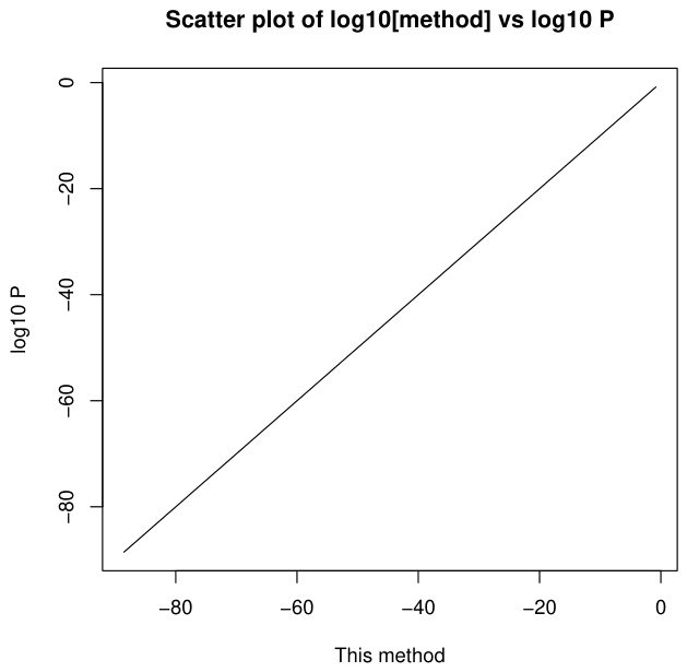
Finally, Figure 4 compares the numerically evaluated tail probability with the theoretical lower and upper bounds and . All numerical results lie strictly within the interval , as required by the analysis in Section 2. For large Z, the three curves become indistinguishable at the scale of double precision, illustrating that classical bounds, numerical integration results, and direct evaluation coincide within rounding error. This agreement provides numerical confirmation of the theoretical decomposition and clarifies the empirical robustness observed in existing implementations.
4.5. Summary
Taken together, these experiments demonstrate that the proposed formulation provides explicit and independent control over underflow, truncation error, and numerical integration error. The observed behavior is fully consistent with the analytical framework developed in Section and explains why Gaussian tail probabilities can be evaluated reliably even in extreme parameter regimes.
5. Discussion
The numerical evaluation of Gaussian tail probabilities is a problem for which highly optimized implementations have long been available. As confirmed by the numerical experiments in Section 4, modern software such as the R implementation of pnorm achieves remarkable numerical robustness, even for extremely large values of Z. In particular, logarithmic–domain evaluations based on rational minimax approximations remain stable and accurate far beyond parameter ranges that would challenge naive numerical approaches.
From the perspective of this study, these findings were initially unexpected. Early versions of the present work were motivated by the possibility that large–Z regimes might expose numerical limitations in standard implementations. Instead, systematic experimentation revealed that such limitations do not manifest in practice within double–precision arithmetic. This outcome does not diminish the relevance of the present analysis; rather, it clarifies the scope and significance of its contribution.
The central contribution of this work lies not in outperforming existing numerical algorithms, but in providing a transparent theoretical framework that explains why they work so well. By reformulating Gaussian tail evaluation as a controlled numerical integration problem, we explicitly decomposed numerical error into three independent components: underflow, truncation error, and numerical integration error. This decomposition makes precise the roles played by scaling, domain truncation, and discretization, respectively. Within this framework, classical analytical bounds such as Mills–type inequalities arise naturally as rigorous enclosures of the true tail probability.
Our analysis demonstrates that phenomena historically regarded as purely algorithmic or empirical—for example, the apparent stability of tail probability evaluations for very large arguments—can be understood as the cumulative effect of well–structured error control mechanisms. In this sense, the present work provides a theoretical underpinning for numerical techniques that have long been known to perform reliably in practice, but whose rationale has remained largely implicit.
It is important to emphasize that this perspective is complementary to, rather than competitive with, existing minimax–based implementations. Rational Chebyshev approximations, as pioneered by Cody and refined in subsequent numerical libraries, represent an optimal solution from the standpoint of floating–point accuracy. The present formulation instead prioritizes interpretability, explicit error accounting, and analytical transparency. These features may be particularly valuable in settings where theoretical guarantees, reproducibility, or method verification are of interest.
More broadly, this study highlights the value of revisiting mature numerical problems from a structural viewpoint. Even when existing implementations are highly successful, theoretical reformulations can elucidate the principles that make such success possible. By bridging classical analytical bounds and modern numerical practice, the present work contributes to a deeper understanding of Gaussian tail evaluation and, more generally, of the relationship between numerical experimentation and theoretical analysis. “
Acknowledgments
This work was supported by JSPS KAKENHI Grant Numbers JP25K22410, JP26K10050 and Yokohama Foundation for Advancement of Medical Science (Medical Digitalization Grant). AI-assisted tools (Microsoft Copilot, 2026) were used solely for idea organization and for improving the clarity and fluency of the English text. All mathematical derivations, theoretical arguments, numerical experiments, and final scientific content were entirely produced and verified by the authors.
Conflicts of Interest
The author declares no conflicts of interest.
References
- Cody, W. J. Rational Chebyshev Approximations for the Error Function. Math. Comput. 1969, vol. 23(no. 107), 631–637. [Google Scholar] [CrossRef]
- Misawa, K. Practical Method for log[ erfc (a)] Approximation in the Extreme Tail; Preprints.org, 2026. [Google Scholar] [CrossRef]
- Shepherd, M. M.; Laframboise, J. G. Chebyshev Approximation of (1+2x)exp(x2)erfc(x) in 0. Math. Comput. 1981, vol. 36(no. 153), 249–253. [Google Scholar] [CrossRef]
- Hastings, C., Jr. Approximations for Digital Computers; Princeton University Press: Princeton, 1955. [Google Scholar]
Figure 1.
Dependence of on Z.
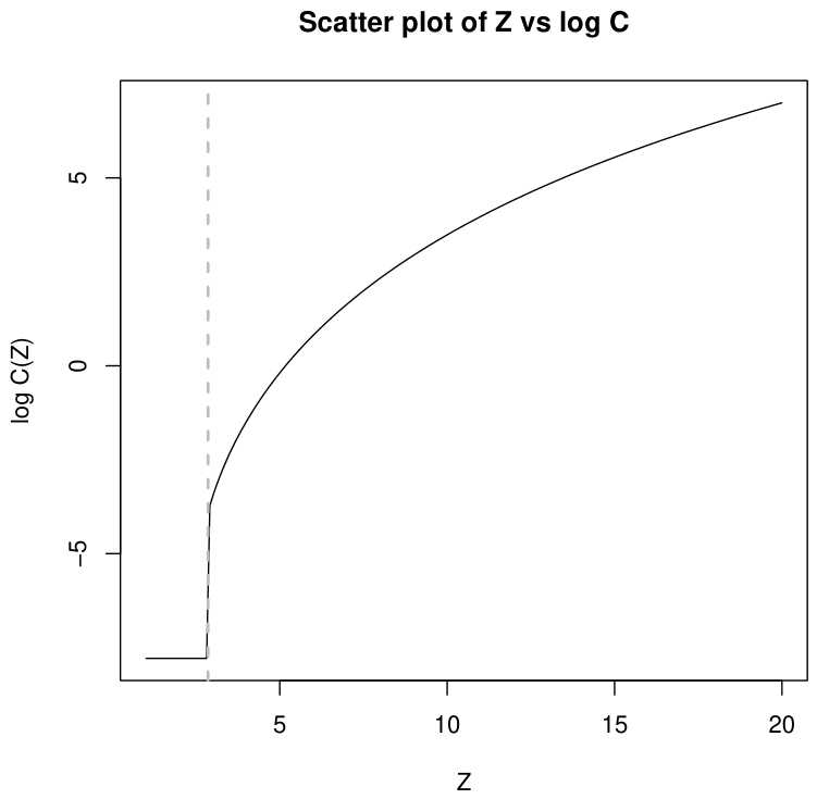
Figure 2.
Integration range determined by truncation error control.
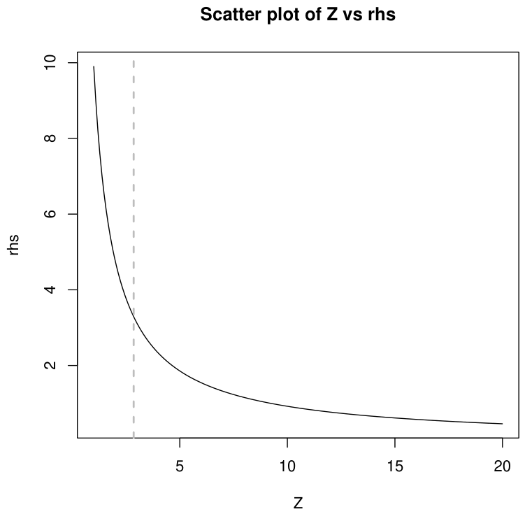
Figure 3.
Number of subdivisions required for numerical integration.
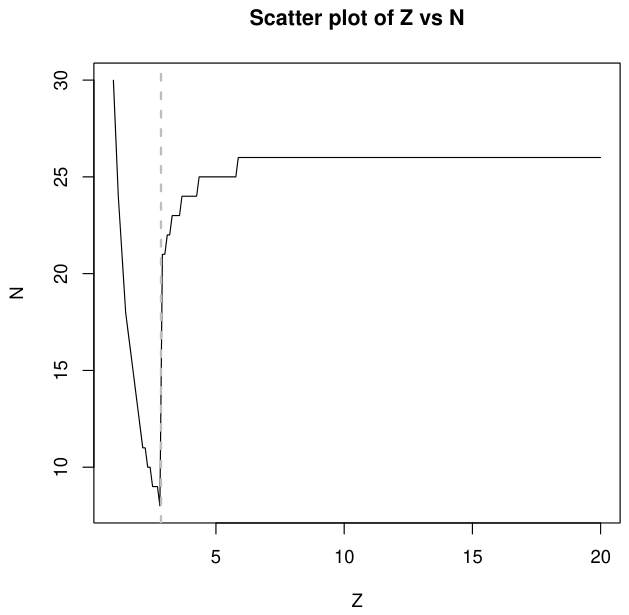
Figure 4.
Comparison of numerical results with the analytical bounds and .
Disclaimer/Publisher’s Note: The statements, opinions and data contained in all publications are solely those of the individual author(s) and contributor(s) and not of MDPI and/or the editor(s). MDPI and/or the editor(s) disclaim responsibility for any injury to people or property resulting from any ideas, methods, instructions or products referred to in the content. |
© 2026 by the authors. Licensee MDPI, Basel, Switzerland. This article is an open access article distributed under the terms and conditions of the Creative Commons Attribution (CC BY) license (http://creativecommons.org/licenses/by/4.0/).
Copyright: This open access article is published under a Creative Commons CC BY 4.0 license, which permit the free download, distribution, and reuse, provided that the author and preprint are cited in any reuse.