
Submitted:
25 September 2026
Posted:
28 September 2026
You are already at the latest version
Abstract
Wave equations with Caputo fractional damping model power-law attenuation in rocks, but their numerical solution is costly because of the non-local memory, and stability proofs for nonlinear variants are error-prone. We study a one-dimensional wave equation with Caputo damping of order α∈(0,1) and a cubic nonlinearity, discretised by Legendre–Gauss–Lobatto (LGL) collocation in space and a linearly implicit three-level scheme with the L1 formula in time. The memory is compressed by a sum-of-exponentials (SOE) approximation with positive weights, which reduces the cost of the history term from O(N2t) to O(NeNt) with Ne growing logarithmically. By a discrete energy argument that does not use a sign of the discrete memory form, we prove stability under a time-step restriction independent of the polynomial degree and an error bound of order τ2-α+N1-m+εSOE; the energy argument is machine-checked in Lean 4. Experiments confirm the temporal rates, spectral accuracy in space and a speed-up of the memory evaluation of up to 60 times. In a seismic application with the damping calibrated from a prescribed quality factor, the quality factor recovered from simulated seismograms agrees with the dispersion relation to within 0.5%. An extension to Caputo’s constitutive model reproduces a nearly constant quality factor.
Keywords:
fractional wave equation
; Caputo derivative
; Legendre–Gauss–Lobatto collocation
; sum-of-exponentials approximation
; energy stability
; formal verification
; Lean 4
; seismic attenuation
and a cubic nonlinearity, discretised by Legendre–Gauss–Lobatto (LGL) collocation in space and a linearly implicit three-level scheme with the L1 formula in time. The memory is compressed by a sum-of-exponentials (SOE) approximation with positive weights, which reduces the cost of the history term from to with growing logarithmically. By a discrete energy argument that does not use a sign of the discrete memory form, we prove stability under a time-step restriction independent of the polynomial degree and an error bound of order ; the energy argument is machine-checked in Lean 4. Experiments confirm the temporal rates, spectral accuracy in space and a speed-up of the memory evaluation of up to 60 times. In a seismic application with the damping calibrated from a prescribed quality factor, the quality factor recovered from simulated seismograms agrees with the dispersion relation to within 0.5%. An extension to Caputo’s constitutive model reproduces a nearly constant quality factor.
1. Introduction
Wave propagation in media with memory, such as porous and fluid-saturated rocks, biological tissue and polymers, is commonly described by integro-differential equations with fractional time derivatives [1,2,3,4,5]. In seismology, fractional models are used to represent intrinsic attenuation and the accompanying velocity dispersion [6,7,8,9,10,11]. Two computational difficulties are characteristic of such models: the fractional operator is non-local in time, so that a direct discretisation requires storing and re-using the whole history, and nonlinear terms complicate the stability analysis.
Spectral methods for linear time-fractional wave and diffusion-wave problems have been studied, e.g., in [12,13,14,15], and a considerable body of work addresses nonlinear time-fractional Klein–Gordon-type equations [16,17,18,19,20,21,22,23,24], and high-order discretisations of related nonlinear fractional models are reported in [25,26]. The memory cost of the Caputo derivative can be reduced by sum-of-exponentials (SOE) or kernel-compression techniques [27,28,29,30], which rest on exponential-sum approximations of the power kernel [31,32].
In this paper we consider a one-dimensional wave equation with Caputo fractional damping of order and a cubic restoring term, discretised by Legendre–Gauss–Lobatto (LGL) collocation in space and by a linearly implicit three-level scheme with the L1 formula in time. The contributions are as follows.
A fast L1–SOE implementation in which the kernel is approximated by an exponentially convergent trapezoidal rule with strictly positive nodes and weights, together with an explicit recursion for the history term.
A stability and convergence analysis based on a discrete energy identity and a bound on the L1 memory operator. The argument does not use a sign of the discrete memory form; we show numerically that, for the pairing with the centred difference that arises in the energy method, this form is indefinite, so that it cannot simply be discarded. The resulting time-step restriction is independent of the polynomial degree .
- A seismic application in which the damping coefficient is calibrated from a prescribed quality factor, the discretisation is verified against an exact solution and against a second-order finite-difference discretisation, and the attenuation law recovered from the simulated seismograms is compared with the dispersion relation of the continuous model.
- An extension of the scheme to Caputo’s constitutive model [4], in which the fractional derivative acts on the strain; this model yields a nearly frequency-independent quality factor, as is typical of rocks.
Individually, LGL collocation, the L1 formula and SOE compression are known; the novelty of this work lies in the stability argument that avoids the sign of the discrete memory form (and in the observation that this sign is not available), in its machine-checked formalisation, and in the quantitative validation of the simulated attenuation law against the continuous dispersion relation for two different fractional attenuation models. The cubic term is used as a phenomenological Klein–Gordon-type nonlinearity, as in [16,17,22]; its physical interpretation is discussed in Section 2.2.
The paper is organised as follows. Section 2 states the problem and analyses the attenuation law of the model. Section 3 describes the scheme and the SOE acceleration. Section 4 contains the stability and convergence analysis and its formalisation. Section 5 reports numerical tests, Section 6 the seismic application, and Section 7 and Section 8 contain a discussion and conclusions.
2. Problem Formulation
Let and . We consider
where is the wave speed, is the damping coefficient, is a source term and is the Caputo derivative of order ,
The nonlinearity is the cubic restoring force with . In the analysis we only use that is locally Lipschitz with .
2.1. Attenuation Law of the Linear Model
For and a plane wave , the (steady-state) Caputo derivative acts as multiplication by , and (1) yields the dispersion relation
Defining the quality factor by we obtain
Three consequences are important for the interpretation of the model. (i) For the damping term becomes the classical viscous term and ; for it becomes , which does not dissipate energy. For fixed and (in particular in the seismic frequency band), the attenuation therefore increases with ; because the unit of depends on (see (iii)), such comparisons at equal depend on the units and are only indicative. (ii) For weak attenuation, , i.e., the model describes a power-law, frequency-dependent attenuation and not a constant- medium; constant- models are obtained by placing a fractional derivative in the stress–strain relation [6,7,35]. (iii) The coefficient is not dimensionless () and must be calibrated. Given a target quality factor at the dominant angular frequency , (5) gives exactly
so that . The order then controls the frequency dependence of around . This calibration is used in Section 6.
2.2. Role of the Cubic Term
The cubic term is an on-site (Klein–Gordon or Duffing-type) nonlinearity. It should not be confused with the nonlinearity of finite-strain elasticity: the Murnaghan–Landau expansion of the elastic energy [36] leads to a nonlinear flux whose leading correction is quadratic in the strain. We therefore regard as a phenomenological model and as a standard benchmark for numerical methods [16,17,22]. For a wave of amplitude and angular frequency , the relative size of the cubic term is measured by
For the strain amplitudes of seismic waves away from the source (), is negligible unless is extremely large; the nonlinear seismic computations in Section 6.5 are therefore a parametric study rather than a prediction for a specific rock.
3. Numerical Scheme
3.1. LGL Collocation in Space
Let be the LGL nodes, i.e., the zeros of , with quadrature weights , and let . Let be the first-order Legendre collocation differentiation matrix [37,38] and let
be the second-derivative matrix restricted to the interior nodes, which incorporates the homogeneous Dirichlet conditions. For we denote by the polynomial interpolating at the interior nodes and vanishing at ; then . We use the discrete inner product and norm
and the stiffness form .
3.2. L1 Approximation of the Caputo Derivative
On the uniform grid , , the L1 formula reads [39]
The weights satisfy and . For the truncation error is . A direct evaluation of (10) costs operations per node at step , hence in total, and requires storing all time levels.
3.3. Fast Evaluation by a Sum of Exponentials
The kernel admits the exact representation
which follows from with . Truncating the integral to and applying the trapezoidal rule with step gives [31,32]
All nodes and weights are strictly positive by construction. The step is reduced until the relative error on , measured on a dense logarithmic grid, is below a prescribed tolerance , and exponentials that are negligible on are removed. For and this gives exponentials for and for (on ), in agreement with the logarithmic growth of with [32].
Following [27], the most recent interval is treated exactly by the L1 formula and the history part by (12). With the piecewise linear interpolant of this gives
where the history variables satisfy the recursion
Indeed, for the piecewise linear interpolant of the time levels, and splitting off the last interval yields (14). The cost per time step is and the memory , independent of .
3.4. Fully Discrete Scheme
Let approximate at the interior nodes. The fully discrete scheme is
where is given by (10) or (13), and the first step is computed from a Taylor expansion,
using that the Caputo term vanishes at . Since and involve only known levels, each step requires the solution of
By Lemma 1 below, the matrix is symmetric positive definite with respect to and hence nonsingular for every ; it is factorised once by LU decomposition.
4. Stability and Convergence
We write , and define the discrete energy
Lemma 1 (Properties of the LGL stiffness matrix). For all : (a) ; in particular is symmetric with respect to and with equality only for ; (b) with ; (c)
Proof. (a) Since has degree and the LGL rule is exact for polynomials of degree , and vanishes at the end points, . (b) For the discrete and continuous norms satisfy [37]; combined with the Poincaré inequality this gives (b). (c) . □
In our implementation the relative deviation of from symmetry, , is for .
Lemma 2 (Discrete energy identity). Let satisfy (15) and set . Then, for
Proof. Take the inner product of (15) with . The identities and, by the symmetry of , telescope the inertial and stiffness terms; dividing by gives the claim. □
Lemma 3 (Bound on the memory operator). Let and . Then
Proof. Since and , the triangle inequality gives . The fast operator (13) has the same structure with the history weights , , replaced by integrals of the SOE kernel over the corresponding intervals. Since the SOE kernel is positive and approximates with relative accuracy on , these weights lie in . □
Remark 1 (On the sign of the memory term). Forone would like to discard the memory contributionin the summed energy identity as non-positive. With, this sum is a quadratic form. The positivity results for the L1 kernel [39,40] concern the pairing with the backward difference only; for the centred pairing the form is indefinite: the smallest eigenvalue of its symmetric part is between and for all and (script exp_memory_form.jl). The analysis below therefore bounds the memory term by Lemma 3 instead of using its sign.
Theorem 1 (Stability). Let , , , and assume that for all . Let
If , then the solution of (15) with the L1 memory (10) satisfies
The same holds for the L1–SOE memory (13) with replaced by
Proof. Fix and let with for . By (18) and Lemma 1, and . Lemma 3 gives , and the Lipschitz bound with Lemma 1(b) gives , so that with . In Lemma 2 we use the Cauchy–Schwarz inequality, and Young’s inequality to obtain , hence and, for , . Taking and arguing by induction gives . For the SOE variant, Lemma 3 is used with . □
The time-step restriction depends on , , , , and , but not on : in contrast to explicit schemes, there is no CFL condition, which matters because the largest eigenvalue of grows like . For and , Lemma 2 shows that is exactly conserved for every .
Corollary 1 (A priori bound for the cubic nonlinearity). Let , , and let be defined with . If and , then for all , and the conclusion of Theorem 1 holds.
Proof. If , then and the Lipschitz assumption holds at level . Conversely, by Lemma 1(c) and (18), . Induction on , using Theorem 1 up to level , gives the claim. □
Corollary 1 is a small-data result; for the defocusing cubic term a modified energy that includes the potential could remove the smallness assumption, but this is not pursued here.
Theorem 2 (Convergence). Let the solution of (1)–(2) satisfy withand, letdenote the-orthogonal projection onto, and let. Then there existand, independent ofand, such that forandsufficiently large
Proof. By Lemma 1(a), the collocation scheme is equivalent to a Galerkin method with numerical integration, since . Hence the error satisfies (15) with , where and the residual is defined by for the consistency functional . Because is the -orthogonal projection, , so that the stiffness term does not contribute to . The remaining contributions are: the truncation errors of the second difference and of the averaged stiffness term, for ; the L1 truncation error, [39]; the projection errors and the LGL quadrature errors for , and , [16,37,38]; and the SOE error, . Since , it follows that . As long as and , . The energy argument of Theorem 1 with the additional residual (formalised as l1_scheme_error_bound, Section 4.1) gives . The starting step (16) yields . The bound on required for the Lipschitz estimate follows by induction from the error bound and Lemma 1(c) for small and large. □
Remark 2 (Regularity). The assumption, needed for theconsistency of the three-level scheme, is standard but restrictive for fractional problems [41,42].For (1) withthe Caputo term behaves likenear, so thatis only Hölder continuous and. The resulting initial layer is milder than for subdiffusion. In the test ofSection 5.2 (unforced problem with ) no loss of the temporal rate atis observed; for stronger singularities graded temporal meshes [41] can be used.
4.1. Machine-Checked Part of the Analysis
The algebraic core of Lemmas 2 and 3 and Theorems 1 and 2 was formalised in Lean 4 [33] using Mathlib [34]. The discrete space with is modelled by an arbitrary real inner-product space, the stiffness operator by a linear map, and the L1 operator (10) is defined explicitly. Table 1 lists the formalised statements. The development contains no sorry, and the command #print axioms reports only the standard axioms propext, Classical.choice and Quot.sound. It was checked with Lean v4.35.0-rc2 and a pinned Mathlib commit (Supplementary Materials).
The following ingredients are assumptions of the formal statements and are proved on paper only: the symmetry and semi-definiteness of and the Poincaré inequality (Lemma 1), the Lipschitz bound on (Corollary 1), the truncation-error estimates in the proof of Theorem 2 and the SOE perturbation bound in Lemma 3. The formalisation thus certifies the energy argument itself, which is the part of such proofs where sign and index errors are most likely.
5. Numerical Experiments
All computations were performed in Julia 1.12.4 with the packages FastGaussQuadrature 1.3.0, SpecialFunctions 2.9.0 and Plots 1.41.7, on a single core of an Intel Core i5-9400F processor (2.9 GHz, 16 GB RAM); the formal proofs were checked with Lean v4.35.0-rc2 and Mathlib (commit b0df0c4). The complete code and the Lean project are provided in the Supplementary Materials and are archived on Zenodo [43]. The generative AI tool Claude (Anthropic, Claude Opus 5) was used for translation and generation of the manuscript text, and to assist in implementing and testing the SOE solver, in developing the Lean 4 formalisation and in producing the figures; all text, code, proofs and results were checked by the authors (see Acknowledgments). To test accuracy we use (1) with , , and the manufactured solution , for which
Errors are measured in the discrete norm at . Unless stated otherwise, the L1–SOE memory with is used.
5.1. Temporal Convergence
Table 2 shows the errors for , for which the spatial error is negligible. Two error components are present: an contribution of the three-level scheme and an contribution of the L1 formula, whose constant is proportional to . For the observed rate increases monotonically towards . For the two contributions have opposite signs and cancel near , which produces the non-monotone behaviour; for larger the rate approaches . For the contribution is smaller than the one over the whole range, and the observed rate is close to 2; the asymptotic rate is not reached before round-off errors, which are amplified like by the second difference, become visible at errors of about .
5.2. Unforced Problem with an Initial Layer
The manufactured solution above is smooth in time. To test the effect of the weak initial singularity discussed in Remark 2, we solve the unforced problem , , with and (, , ). Since the exact solution is not available in closed form, and a very fine reference solution would be contaminated by round-off (Section 5.1), we use the self-convergence differences , which behave like the error for a fixed asymptotic rate. Table 3 shows the results for . For and the observed rates approach as for the smooth solution; for the component again dominates. The results for are similar (script exp_initial_layer.jl). Thus the initial layer does not reduce the rate at in this test.
5.3. Spatial Convergence
5.4. Efficiency of the SOE Acceleration
Table 4 compares the CPU time spent on the memory term for the direct L1 formula and the L1–SOE formula (, ; best of three runs). The two solutions agree to within in the relative discrete norm, far below the discretisation error. The direct evaluation grows quadratically with (the growth beyond a factor of four between the last two rows is due to cache effects), whereas the SOE evaluation grows linearly. The SOE variant becomes faster than the direct one at – and is times faster for and times faster for . In addition, the SOE variant stores history vectors instead of .
5.5. Energy Behaviour
Figure 2 shows the discrete energy for a Gaussian pulse , , , , , , , without and with the cubic term. In the nonlinear case we take , for which the cubic term is comparable to the stiffness term, and add the discrete potential to . At the energy is , and of its initial value for , and in the linear case, and , and with the cubic term; the nonlinearity changes the energy balance only slightly. For this dimensionless problem the dominant frequencies satisfy , so the stronger decay for larger agrees with Section 2.1. The decay is not strictly monotone: on individual steps the energy may increase by up to , which is consistent with Remark 1 and with Theorem 1, which only asserts a bound.
6. Application to Seismic Wave Attenuation
6.1. Set-Up and Verification
We consider a 10 km profile with m/s and an initial Ricker wavelet , , with Hz, km and . The amplitude is normalised to one. The wavelet splits into two pulses travelling in opposite directions, which reach the boundaries after s; with s the results are free of boundary reflections. The parameters are listed in Table 5. Receiver traces are obtained by barycentric interpolation of the LGL solution.
The discretisation parameters were chosen by comparison with the exact elastic solution (, ) at receivers at 6, 7 and 8 km (Table 6). With the pulse is severely under-resolved (relative error 77%) and the numerical solution exhibits spurious dispersive wakes; for the spatial error is negligible and the remaining error is temporal and decreases at second order. The choice , gives a relative error of .
6.2. Attenuation in Three Media
We fix and calibrate by (6) to , and at Hz, illustrative values for strongly attenuating unconsolidated or hydrate-bearing sediments, sandstone and crystalline rock, respectively; this gives , and . Figure 3 shows the wavefield at s and Figure 4 the peak amplitude as a function of the propagation distance, normalised by the elastic peak. The dashed lines show the plane-wave prediction at the dominant frequency. The agreement is close for and ; for the deviations reflect the broadband nature of the pulse and the frequency dependence of , which shifts the dominant frequency during propagation. Figure 5 shows the space–time wavefield for .
6.3. Validation of the Attenuation Law
To test whether the discretisation reproduces the attenuation law of the continuous model, we calibrate to at 10 Hz for , and and record the right-going pulse at km and km. The attenuation coefficient is estimated from the spectral ratio, , and converted into , where is the root of (4) with . Figure 6 compares with . At 10 Hz the measured values are , and (theory: ), and the maximal relative deviation between 5 and 20 Hz is , and for , and . Thus the scheme reproduces the attenuation law, including its frequency dependence , and the transient memory effects of the Caputo initial-value problem are negligible at these offsets.
6.4. Influence of the Fractional Order
Although the three media in Section 6.3 have the same at 10 Hz, their seismograms differ considerably (Figure 7). For the quality factor varies from about 4 at 4 Hz to about 130 at 22 Hz (Figure 6), so that low frequencies are strongly suppressed and the pulse becomes narrower-band and oscillatory, with a pronounced trailing wavelet and a phase shift due to velocity dispersion; for the frequency dependence is weaker and the pulse shape is closer to the elastic one. Hence is not determined by the value of at a single frequency: it has to be constrained by the observed frequency dependence of attenuation.
6.5. Effect of the Cubic Term
Finally, Figure 8 shows seismograms at km for the sandstone model (, ) with and , and (see (7) with ). The relative difference from the linear seismogram is for and for . The cubic term shifts the main phase to earlier times, reduces its period and, for , generates a slowly decaying tail. As discussed in Section 2.2, such values of require a very strong on-site nonlinearity; the computation illustrates the robustness of the scheme in a moderately nonlinear regime rather than a quantitative prediction.
6.6. Comparison with a Finite-Difference Discretisation
To quantify the benefit of the spectral discretisation, we replace the LGL matrix by the standard second-order finite-difference matrix on a uniform grid with intervals and keep the time integrator unchanged. For the elastic test of Section 6.1 with (temporal error about ), Table 7 and Figure 9 compare the relative receiver errors and the CPU times. The LGL scheme reaches an error of with unknowns in 1.3 s, whereas the finite-difference scheme needs intervals and 11.1 s for the same accuracy; with the LGL error reaches the temporal error level. The finite-difference matrix is sparse, so its cost per step is lower, but the number of unknowns required for a given accuracy is larger by a factor of about 50. The advantage of the spectral method grows with the required accuracy and with the number of wavelengths in the domain.
6.7. Extension to Caputo’s Constitutive Model
As discussed in Section 2.1, the damping model (1) yields , whereas the attenuation of rocks is often nearly frequency independent. A classical model with this property is Caputo’s constitutive law [1,4], in which the fractional derivative acts on the strain:
For a plane wave, the complex modulus is and
where the second relation calibrates . Since for weak attenuation, small gives a nearly constant . The scheme of Section 3 carries over with one modification: because the constitutive term contains the unbounded operator , it is averaged like the stiffness term, , and the local L1 part of is treated implicitly. The system matrix becomes , which is again constant and symmetric positive definite with respect to ; the history part is evaluated with the same SOE recursion. The stability analysis of Section 4 does not cover this variant, and its stability is observed numerically.
Figure 10 shows the quality factor measured from simulated seismograms (set-up of Section 6.3, , ) for at 10 Hz. For , varies only from 31.7 at 5 Hz to 28.4 at 20 Hz, and the measured values agree with (21) to within between 5 and 20 Hz for both and ; direct L1 and L1–SOE solutions agree to within . The seismograms show two differences from the damping model with the same at 10 Hz. First, the pulse retains a Ricker-like, broadened shape without the oscillatory trailing wavelet of the damping model. Second, it arrives earlier: the modulus exceeds one, so that the phase velocity at 10 Hz is about for and for . In applications, should therefore be chosen such that the phase velocity at matches the observed velocity, in addition to the calibration of .
7. Discussion
The analysis in Section 4 differs from arguments in which the discrete memory term is discarded as dissipative. Remark 1 shows that the corresponding quadratic form is indefinite for the centred pairing of the three-level scheme, and Figure 2 confirms that the discrete energy is not strictly monotone. Bounding the memory term instead (Lemma 3) leads to an exponential factor in the stability bound, and grows like . For the test problems of Section 5 the constants are moderate (). For the seismic runs, however, the calibrated coefficients are large: for and , , and one obtains , , and , and for , even . The step-size condition of Theorem 1 is therefore violated in some of the simulations of Section 6, and where it holds the bound is far too large to be informative. The stability of these computations is thus an empirical observation, supported by the verification against the exact solution and by the agreement of the measured attenuation with the dispersion relation, and not a consequence of Theorem 1. A sharper analysis that exploits the dissipativity of the continuous operator, for instance by pairing the memory term with a backward difference in a modified scheme, is an interesting direction.
The formalisation covers the energy argument, i.e., the part of the proof in which algebraic errors are most likely to go unnoticed. The approximation-theoretic ingredients (LGL quadrature, projection and truncation error estimates, SOE approximation) are assumed. Formalising them would require substantial additional libraries.
The physical interpretation of the model requires care. The damping term produces a power-law attenuation with and not a constant ; for fixed the attenuation grows with , and only a calibration such as (6) makes the parameters comparable across media. For nearly constant- modelling, the fractional derivative should be placed in the constitutive relation [6,7,8,35]. Section 6.7 shows that the LGL discretisation and the SOE compression carry over to Caputo’s constitutive model and reproduce its attenuation law; extending the energy analysis to this model, whose memory term involves the unbounded operator , remains open. The resolution study in Section 6.1 shows that under-resolved spectral simulations produce dispersive wakes that can be mistaken for physical dispersion; convergence studies should therefore accompany applications of fractional wave models.
Section 6.6 shows that, for a propagation distance of several wavelengths, the spectral discretisation needs about 50 times fewer unknowns than a second-order finite-difference scheme and is about eight times faster for the same accuracy. The main limitations are the restriction to one space dimension, the small-data assumption in Corollary 1, the use of Dirichlet boundaries on a large domain instead of absorbing boundaries, and the reduced temporal order of the L1 formula. Natural extensions are tensor-product LGL or spectral-element discretisations in two and three dimensions, perfectly matched layers or absorbing boundary conditions [44,45,46], graded meshes [41], and second-order formulas such as [17].
8. Conclusions
We have presented an LGL spectral collocation method with a fast L1–SOE treatment of the Caputo damping term for a one-dimensional nonlinear fractional wave equation. The scheme is linearly implicit, requires one LU factorisation, and its memory cost grows only logarithmically with the number of time steps. We proved stability under a time-step restriction independent of the polynomial degree and an error bound of order , without relying on a sign of the discrete memory form, and we machine-checked the energy argument in Lean 4. The numerical experiments confirm the temporal rates, spectral accuracy in space and speed-ups of the memory evaluation of up to 60 times. In the seismic application the damping coefficient was calibrated from a prescribed quality factor, and the quality factor recovered from simulated seismograms agreed with the dispersion relation to within 0.5%. Compared with second-order finite differences, the spectral scheme required about 50 times fewer unknowns and was about eight times faster at equal accuracy, and the method carries over to Caputo’s constitutive model, whose nearly constant quality factor it reproduces to within 0.02%.
Supplementary Materials
The following supporting information can be downloaded at: https://www.mdpi.com/article/doi/s1, Code S1: Julia source code (JuliaSim.zip) reproducing all tables and figures, including the LGL-L1-SOE solver, the SOE construction and all experiment scripts; Code S2: Lean 4 project (Lean4_Verification.zip) containing the machine-checked proofs listed in Table 1. Both archives are also available on Zenodo at https://doi.org/10.5281/zenodo.22880395.
Author Contributions
Conceptualization, Z.A. and Y.K.; Methodology, Z.A.; Software, N.A. and Z.A.; Validation, Y.K. and N.A.; Formal Analysis, Z.A.; Investigation, Y.K. and N.A.; Visualization, Y.K. and N.A.; Writing – Original Draft Preparation, Z.A.; Writing – Review & Editing, Y.K., N.A. and A.B.; Supervision, A.B.; Funding Acquisition, Z.A. All authors have read and agreed to the published version of the manuscript.
Funding
This research was funded by the Science Committee of the Ministry of Science and Higher Education of the Republic of Kazakhstan, grant number AP22683307.
Data Availability Statement
The original data presented in the study are openly available in Zenodo at https://doi.org/10.5281/zenodo.22880395 [43], which contains the code and the Lean 4 project that reproduce all reported data; they are also included in the Supplementary Materials (Codes S1 and S2).
Acknowledgments
During the preparation of this manuscript, the authors used Claude (Anthropic, Claude Opus 5) for the purposes of translation and generation of the manuscript text, developing the Lean 4 formalisation. The authors have reviewed and edited the output and take full responsibility for the content of this publication.
Conflicts of Interest
The authors declare no conflicts of interest. The funders had no role in the design of the study; in the collection, analyses, or interpretation of data; in the writing of the manuscript; or in the decision to publish the results.
Abbreviations
The following abbreviations are used in this manuscript:
| LGL | Legendre–Gauss–Lobatto |
| SOE | Sum of exponentials |
| L1 | L1 approximation of the Caputo derivative |
| CFL | Courant–Friedrichs–Lewy |
References
- Mainardi, F. Fractional Calculus and Waves in Linear Viscoelasticity; Imperial College Press: London, UK, 2010. [Google Scholar] [CrossRef]
- Szabo, T.L.; Wu, J. A model for longitudinal and shear wave propagation in viscoelastic media. J. Acoust. Soc. Am. 2000, 107, 2437–2446. [Google Scholar] [CrossRef]
- Holm, S. Waves with Power-Law Attenuation; Springer: Cham, Switzerland, 2019. [Google Scholar] [CrossRef]
- Caputo, M. Linear models of dissipation whose Q is almost frequency independent—II. Geophys. J. Int. 1967, 13, 529–539. [Google Scholar] [CrossRef]
- Zhao, X.; McGough, R.J. Time-domain comparisons of power law attenuation in causal and noncausal time-fractional wave equations. J. Acoust. Soc. Am. 2016, 139, 3021–3031. [Google Scholar] [CrossRef]
- Carcione, J.M.; Cavallini, F.; Mainardi, F.; Hanyga, A. Time-domain modeling of constant-Q seismic waves using fractional derivatives. Pure Appl. Geophys. 2002, 159, 1719–1736. [Google Scholar] [CrossRef]
- Zhu, T.; Harris, J.M. Modeling acoustic wave propagation in heterogeneous attenuating media using decoupled fractional Laplacians. Geophysics 2014, 79, T105–T116. [Google Scholar] [CrossRef]
- Xing, G.; Zhu, T. Modeling frequency-independent Q viscoacoustic wave propagation in heterogeneous media. J. Geophys. Res. Solid Earth 2019, 124, 11568–11584. [Google Scholar] [CrossRef]
- Wang, Y.; Ning, Y.; Wang, Y. Fractional time derivative seismic wave equation modeling for natural gas hydrate. Energies 2020, 13, 5901. [Google Scholar] [CrossRef]
- Song, G.; Zhang, X.; Wang, Z.; Chen, Y.; Chen, P. The asymptotic local finite-difference method of the fractional wave equation and its viscous seismic wavefield simulation. Geophysics 2020, 85, T179–T189. [Google Scholar] [CrossRef]
- Qiao, Z.; Sun, C.; Wu, D. Theory and modelling of constant-Q viscoelastic anisotropic media using fractional derivative. Geophys. J. Int. 2019, 217, 798–815. [Google Scholar] [CrossRef]
- Yang, Y.; Chen, Y.; Huang, Y.; Wei, H. Spectral collocation method for the time-fractional diffusion-wave equation and convergence analysis. Comput. Math. Appl. 2017, 73, 1218–1232. [Google Scholar] [CrossRef]
- Kamran; Shah, F.A.; Shah, K.; Abdeljawad, T. Numerical solution of two-dimensional time-fractional telegraph equation using Chebyshev spectral collocation method. Partial Differ. Equ. Appl. Math. 2025, 13, 101129. [Google Scholar] [CrossRef]
- Gutleb, T.S.; Carrillo, J.A. A static memory sparse spectral method for time-fractional PDEs. J. Comput. Phys. 2023, 494, 112522. [Google Scholar] [CrossRef]
- Shiyapov, K.; Abdiramanov, Z.; Issa, Z.; Zhumaseyitova, A. High-order spectral scheme with structure maintenance and fast memory algorithm for nonlocal nonlinear diffusion equations. AppliedMath 2026, 6, 54. [Google Scholar] [CrossRef]
- Chen, H.; Lü, S.; Chen, W. A fully discrete spectral method for the nonlinear time fractional Klein-Gordon equation. Taiwan. J. Math. 2017, 21, 231–251. [Google Scholar] [CrossRef]
- Lyu, P.; Vong, S. A linearized second-order scheme for nonlinear time fractional Klein-Gordon type equations. Numer. Algorithms 2018, 78, 485–511. [Google Scholar] [CrossRef]
- Vong, S.; Wang, Z. A compact difference scheme for a two dimensional fractional Klein-Gordon equation with Neumann boundary conditions. J. Comput. Phys. 2014, 274, 268–282. [Google Scholar] [CrossRef]
- Liao, H.-L.; Liu, N.; Lyu, P. Discrete gradient structure of a second-order variable-step method for nonlinear integro-differential models. SIAM J. Numer. Anal. 2023, 61, 2157–2181. [Google Scholar] [CrossRef]
- Wang, N.; Shi, D. Two efficient spectral methods for the nonlinear fractional wave equation in unbounded domain. Math. Comput. Simul. 2021, 185, 696–718. [Google Scholar] [CrossRef]
- Taherkhani, S.; Najafi, I.; Ghayebi, B. A pseudospectral Sinc method for numerical investigation of the nonlinear time-fractional Klein-Gordon and sine-Gordon equations. Comput. Methods Differ. Equ. 2023, 11, 357–368. [Google Scholar] [CrossRef]
- Bentrcia, T.; Mennouni, A. On the solution behavior of a nonlinear time-fractional Klein–Gordon equation: Theoretical study and numerical validation. Commun. Nonlinear Sci. Numer. Simul. 2023, 125, 107384. [Google Scholar] [CrossRef]
- Abdiramanov, Z.A.; Baishemirov, Z.D.; Berdyshev, A.S.; Shiyapov, K.M. An implicit difference scheme for a mixed problem of hyperbolic type with memory. Lobachevskii J. Math. 2024, 45, 569–577. [Google Scholar] [CrossRef]
- Huntul, M.J.; Kamran; Shah, F.A. Computational modeling of wave propagation phenomena via a fractional Klein-Gordon equation with modified Atangana-Baleanu-Caputo derivative. Ain Shams Eng. J. 2026, 17, 104039. [Google Scholar] [CrossRef]
- Safari, F.; Zaky, M.A.; Fardi, M.; Hong, C. Fast and accurate high-order discretization of nonlinear fractional integro-differential equations in multi-dimensional settings. Int. Commun. Heat Mass Transf. 2026, 175, 111204. [Google Scholar] [CrossRef]
- Fardi, M.; Safari, F. Numerical analysis of 3D space-fractional neutral-type delayed reaction-diffusion equations using a high-order difference technique. Math. Comput. Simul. 2026, 247, 75–92. [Google Scholar] [CrossRef]
- Jiang, S.; Zhang, J.; Zhang, Q.; Zhang, Z. Fast evaluation of the Caputo fractional derivative and its applications to fractional diffusion equations. Commun. Comput. Phys. 2017, 21, 650–678. [Google Scholar] [CrossRef]
- Baffet, D.; Hesthaven, J.S. A kernel compression scheme for fractional differential equations. SIAM J. Numer. Anal. 2017, 55, 496–520. [Google Scholar] [CrossRef]
- Xiong, Y.; Guo, X. A short-memory operator splitting scheme for constant-Q viscoelastic wave equation. J. Comput. Phys. 2022, 449, 110796. [Google Scholar] [CrossRef]
- Guo, X.; Jiang, S.; Xiong, Y.; Zhang, J. Compressing the memory variables in constant-Q viscoelastic wave propagation via an improved sum-of-exponentials approximation. J. Comput. Phys. 2024, 518, 113326. [Google Scholar] [CrossRef]
- Beylkin, G.; Monzón, L. Approximation by exponential sums revisited. Appl. Comput. Harmon. Anal. 2010, 28, 131–149. [Google Scholar] [CrossRef]
- McLean, W. Exponential sum approximations for t−β. In Contemporary Computational Mathematics—A Celebration of the 80th Birthday of Ian Sloan; Springer: Cham, Switzerland, 2018; pp. 911–930. [Google Scholar] [CrossRef]
- de Moura, L.; Ullrich, S. The Lean 4 theorem prover and programming language. In Automated Deduction—CADE 28; Springer: Cham, Switzerland, 2021; pp. 625–635. [Google Scholar] [CrossRef]
- The mathlib Community. The Lean mathematical library. In Proceedings of the 9th ACM SIGPLAN International Conference on Certified Programs and Proofs (CPP 2020), New Orleans, LA, USA, 20–21 January 2020; pp. 367–381. [Google Scholar] [CrossRef]
- Kjartansson, E. Constant Q-wave propagation and attenuation. J. Geophys. Res. 1979, 84, 4737–4748. [Google Scholar] [CrossRef]
- Landau, L.D.; Lifshitz, E.M. Theory of Elasticity, 3rd ed.; Pergamon Press: Oxford, UK, 1986. [Google Scholar]
- Canuto, C.; Hussaini, M.Y.; Quarteroni, A.; Zang, T.A. Spectral Methods: Fundamentals in Single Domains; Springer: Berlin/Heidelberg, Germany, 2006. [Google Scholar] [CrossRef]
- Shen, J.; Tang, T.; Wang, L.-L. Spectral Methods: Algorithms, Analysis and Applications; Springer: Berlin/Heidelberg, Germany, 2011. [Google Scholar] [CrossRef]
- Jin, B.; Lazarov, R.; Zhou, Z. An analysis of the L1 scheme for the subdiffusion equation with nonsmooth data. IMA J. Numer. Anal. 2016, 36, 197–221. [Google Scholar] [CrossRef]
- Alikhanov, A.A. A new difference scheme for the time fractional diffusion equation. J. Comput. Phys. 2015, 280, 424–438. [Google Scholar] [CrossRef]
- Stynes, M.; O’Riordan, E.; Gracia, J.L. Error analysis of a finite difference method on graded meshes for a time-fractional diffusion equation. SIAM J. Numer. Anal. 2017, 55, 1057–1079. [Google Scholar] [CrossRef]
- Li, B.; Wang, T.; Xie, X. Analysis of the L1 scheme for fractional wave equations with nonsmooth data. Comput. Math. Appl. 2021, 90, 1–12. [Google Scholar] [CrossRef]
- Adil, N.; Kazez, Y.; Berdyshev, A.; Abdiramanov, Z. Code and Lean 4 Proofs for: Fast Spectral Simulation of One-Dimensional Nonlinear Fractional Waves in Attenuating Media, version 1.0.0 [Software]; Zenodo, 2026. [Google Scholar] [CrossRef]
- Berenger, J.-P. A perfectly matched layer for the absorption of electromagnetic waves. J. Comput. Phys. 1994, 114, 185–200. [Google Scholar] [CrossRef]
- Engquist, B.; Majda, A. Absorbing boundary conditions for numerical simulation of waves. Proc. Natl. Acad. Sci. USA 1977, 74, 1765–1766. [Google Scholar] [CrossRef]
- Antoine, X.; Lorin, E. Towards perfectly matched layers for time-dependent space fractional PDEs. J. Comput. Phys. 2019, 391, 59–90. [Google Scholar] [CrossRef]
Figure 1.
Spatial convergence for , , . The plateau for is the temporal error. LGL, Legendre–Gauss–Lobatto; L1, L1 approximation of the Caputo derivative; SOE, sum of exponentials.
Figure 1.
Spatial convergence for , , . The plateau for is the temporal error. LGL, Legendre–Gauss–Lobatto; L1, L1 approximation of the Caputo derivative; SOE, sum of exponentials.
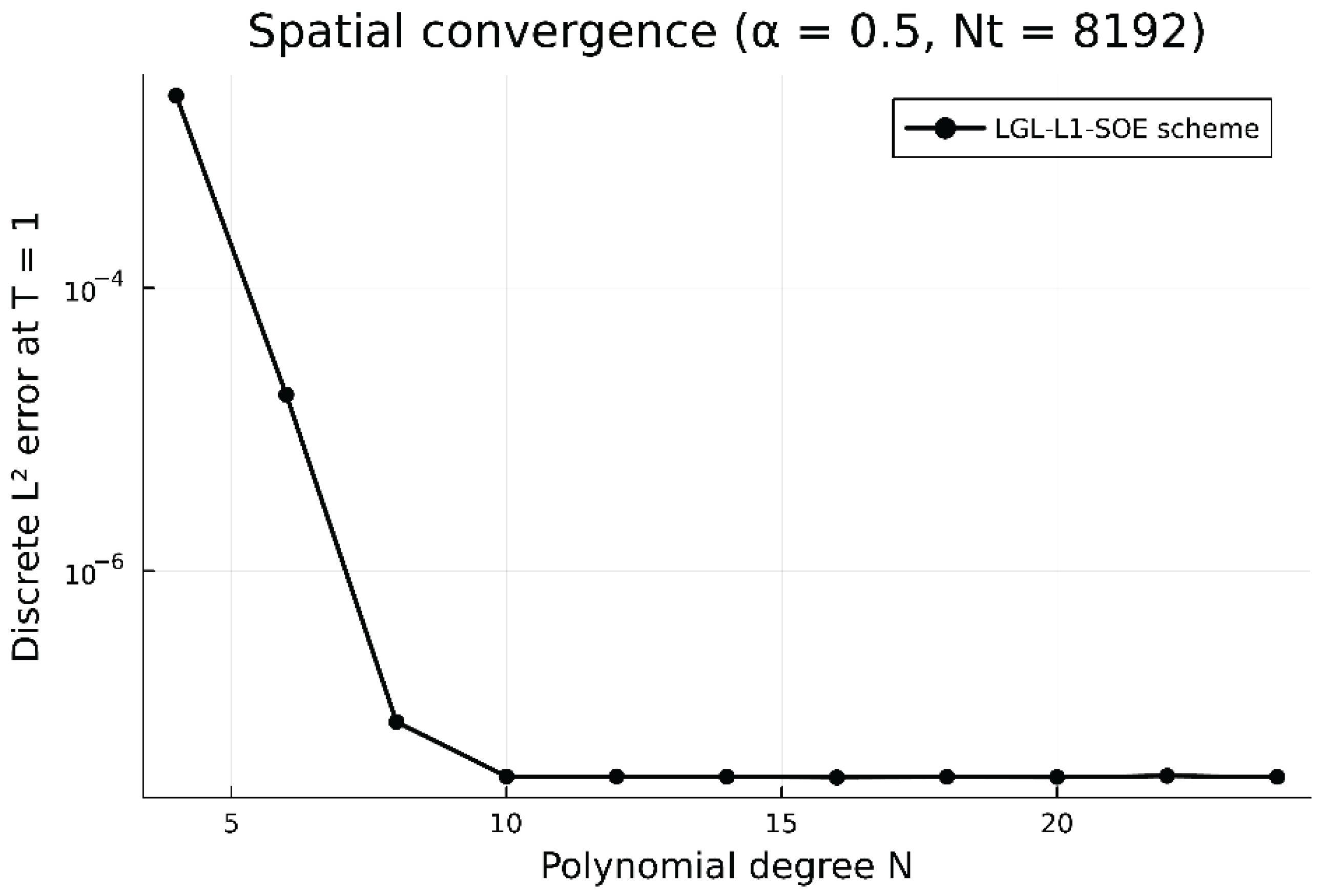
Figure 2.
Discrete energy (normalised by its initial value) for without (dotted) and with (solid, , including the discrete potential) the cubic term.
Figure 2.
Discrete energy (normalised by its initial value) for without (dotted) and with (solid, , including the discrete potential) the cubic term.
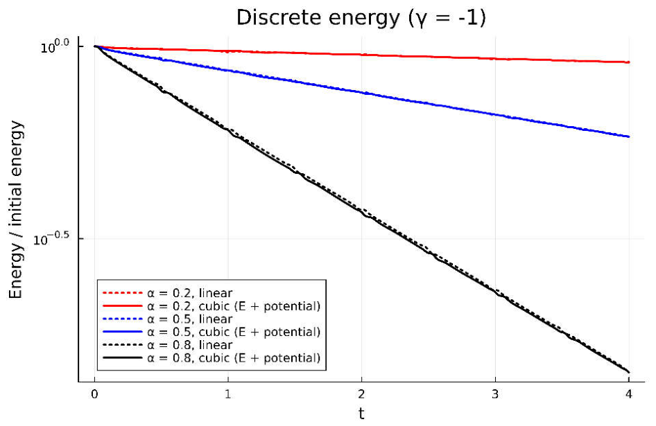
Figure 3.
Wavefield at s for and (right-going pulse); dashed: elastic reference.
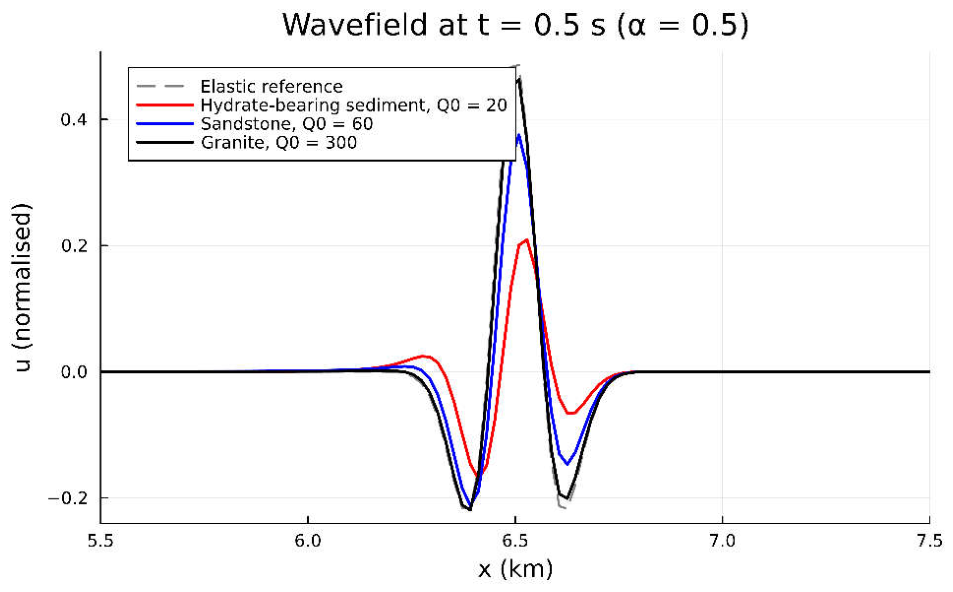
Figure 4.
Peak amplitude normalised by the elastic peak versus propagation distance (solid) and plane-wave prediction at (dashed).
Figure 4.
Peak amplitude normalised by the elastic peak versus propagation distance (solid) and plane-wave prediction at (dashed).
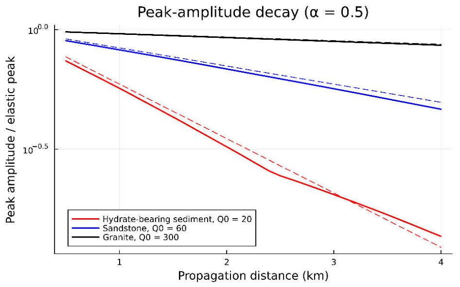
Figure 5.
Space–time wavefield for , .
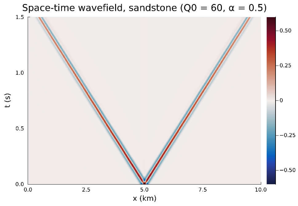
Figure 6.
Quality factor measured from simulated seismograms (markers) and from the dispersion relation (lines) for at 10 Hz.
Figure 6.
Quality factor measured from simulated seismograms (markers) and from the dispersion relation (lines) for at 10 Hz.
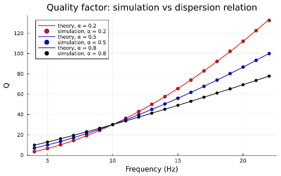
Figure 7.
Seismograms at km for at 10 Hz and ; dashed: exact elastic solution.
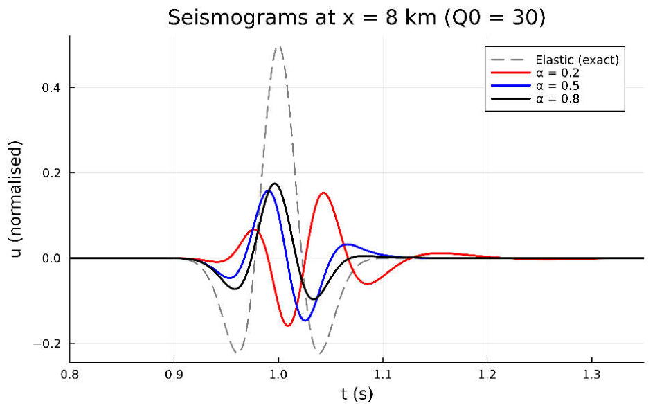
Figure 8.
Seismograms at km for , and nonlinearity strength .
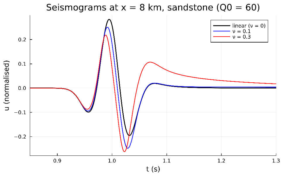
Figure 9.
Elastic Ricker test: relative receiver error versus the number of unknowns (left) and versus CPU time (right) for LGL collocation and second-order finite differences (FD) with the same time integrator.
Figure 9.
Elastic Ricker test: relative receiver error versus the number of unknowns (left) and versus CPU time (right) for LGL collocation and second-order finite differences (FD) with the same time integrator.
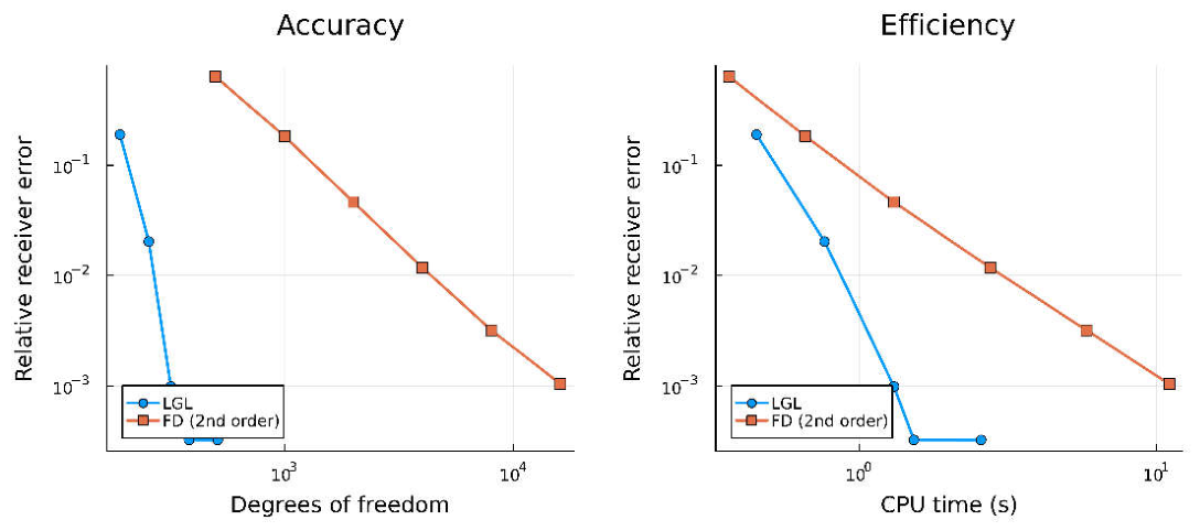
Figure 10.
Caputo’s constitutive model with at 10 Hz: quality factor measured from simulated seismograms (markers) and from (21) (lines), left; seismograms at km compared with the damping model (1) with and the exact elastic solution, right.
Figure 10.
Caputo’s constitutive model with at 10 Hz: quality factor measured from simulated seismograms (markers) and from (21) (lines), left; seismograms at km compared with the damping model (1) with and the exact elastic solution, right.
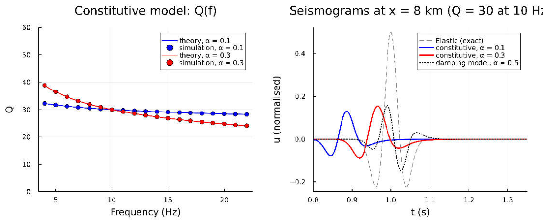

Table 1.
Formalised results (file SnArticleProj.lean in the Supplementary Materials). L1, L1 approximation of the Caputo derivative.
Table 1.
Formalised results (file SnArticleProj.lean in the Supplementary Materials). L1, L1 approximation of the Caputo derivative.
| Lean declaration | Statement | Manuscript |
| energy_identity | Lemma 2 | |
| l1w_nonneg, l1w_sum | Section 3.2 | |
| memL1_bound | Lemma 3 | |
| discrete_growth | discrete Grönwall-type lemma | Theorem 1 |
| energy_estimate(_exp) | energy bound with residual | Theorems 1, 2 |
| l1_scheme_stability | Theorem 1 for the L1 scheme | Theorem 1 |
| l1_scheme_error_bound | error-energy bound | Theorem 2 |
Table 2.
Temporal convergence, , , , L1 formula with sum-of-exponentials (SOE) memory, .
| ) | Rate | ) | Rate | ) | Rate | |
| 256 | 9.38e−6 | – | 2.71e−6 | – | 2.42e−5 | – |
| 512 | 2.23e−6 | 2.07 | 1.87e−7 | 3.86 | 1.15e−5 | 1.07 |
| 1024 | 5.23e−7 | 2.09 | 3.52e−7 | −0.91 | 5.10e−6 | 1.17 |
| 2048 | 1.20e−7 | 2.12 | 1.96e−7 | 0.85 | 2.18e−6 | 1.23 |
| 4096 | 2.67e−8 | 2.17 | 8.72e−8 | 1.17 | 9.11e−7 | 1.26 |
| 8192 | 5.93e−9 | 2.17 | 3.50e−8 | 1.32 | 3.76e−7 | 1.28 |
| 16,384 | 1.63e−9 | 1.86 | 1.31e−8 | 1.42 | 1.54e−7 | 1.29 |
Table 3.
Self-convergence differences and observed rates for the unforced problem with .
| ) | Rate | ) | Rate | ) | Rate | |
| 512 | 7.73e−7 | 2.15 | 7.04e−7 | 0.41 | 5.46e−6 | 1.16 |
| 1024 | 1.69e−7 | 2.20 | 3.42e−7 | 1.04 | 2.35e−6 | 1.22 |
| 2048 | 3.47e−8 | 2.28 | 1.44e−7 | 1.25 | 9.84e−7 | 1.25 |
| 4096 | 6.53e−9 | 2.41 | 5.66e−8 | 1.35 | 4.08e−7 | 1.27 |
| 8192 | 1.21e−9 | 2.43 | 2.12e−8 | 1.42 | 1.67e−7 | 1.29 |
Table 4.
CPU time of the memory term (seconds, single core), , , . The total times include the construction of the SOE approximation, which dominates for small .
Table 4.
CPU time of the memory term (seconds, single core), , , . The total times include the construction of the SOE approximation, which dominates for small .
| Direct L1 | L1–SOE | Speed-up | Total, direct | Total, SOE | Rel. difference | ||
| 1024 | 122 | 0.005 | 0.005 | 0.9 | 0.011 | 0.041 | 3.0e−11 |
| 2048 | 124 | 0.021 | 0.010 | 2.1 | 0.034 | 0.030 | 3.0e−11 |
| 4096 | 126 | 0.084 | 0.021 | 4.0 | 0.110 | 0.056 | 3.0e−11 |
| 8192 | 127 | 0.349 | 0.041 | 8.4 | 0.404 | 0.100 | 3.2e−11 |
| 16,384 | 129 | 1.633 | 0.085 | 19.1 | 1.749 | 0.199 | 4.0e−11 |
| 32,768 | 131 | 10.362 | 0.172 | 60.2 | 10.653 | 0.384 | 1.5e−11 |
Table 5.
Parameters of the seismic simulations.
| Parameter | Value | Parameter | Value |
| 10 km | 768 | ||
| 3000 m/s | 6000 | ||
| 10 Hz | |||
| 1.5 s | Calibration | Equation (6) |
Table 6.
Relative error of receiver traces for the elastic case with respect to the exact solution.
| Relative error | ||
| 128 | 3000 | 7.7e−1 |
| 256 | 3000 | 2.9e−2 |
| 384 | 3000 | 2.1e−2 |
| 512 | 3000 | 2.1e−2 |
| 768 | 3000 | 2.1e−2 |
| 512 | 1500 | 8.2e−2 |
| 512 | 6000 | 5.2e−3 |
| 768 | 6000 | 5.2e−3 |
Table 7.
Relative receiver error and CPU time (single core) for the elastic Ricker test, .
| Error | Time (s) | Error | Time (s) | ||
| 192 | 1.9e−1 | 0.45 | 1000 | 1.8e−1 | 0.66 |
| 256 | 2.0e−2 | 0.77 | 2000 | 4.6e−2 | 1.31 |
| 320 | 9.9e−4 | 1.31 | 4000 | 1.2e−2 | 2.76 |
| 384 | 3.2e−4 | 1.53 | 8000 | 3.2e−3 | 5.82 |
| 512 | 3.2e−4 | 2.57 | 16,000 | 1.0e−3 | 11.05 |
Disclaimer/Publisher’s Note: The statements, opinions and data contained in all publications are solely those of the individual author(s) and contributor(s) and not of MDPI and/or the editor(s). MDPI and/or the editor(s) disclaim responsibility for any injury to people or property resulting from any ideas, methods, instructions or products referred to in the content. |
© 2026 by the authors. Licensee MDPI, Basel, Switzerland. This article is an open access article distributed under the terms and conditions of the Creative Commons Attribution (CC BY) license.
Copyright: This open access article is published under a Creative Commons CC BY 4.0 license, which permit the free download, distribution, and reuse, provided that the author and preprint are cited in any reuse.