

Submitted:
25 September 2026
Posted:
28 September 2026
You are already at the latest version
Abstract
This paper analyzes a GI/M/1/N retrial queue with multiple working vacations, Bernoulli feedback, and impatient customers with retention. Customers who find the server busy do not wait in a physical queue; they join a retrial orbit in which the total retrial attempt rate is proportional to the orbit size (the classical linear retrial policy, rη). Using the supplementary variable technique combined with an embedded Markov chain at arrival epochs, we derive the steady-state distributions at pre-arrival and arbitrary epochs, and we obtain closed-form expressions for the matrix exponentials required for deterministic, Erlang, and hyperexponential inter-arrival times. A degenerate-limit result shows that, as the retrial rate tends to infinity, the model reduces in distribution to the classical GI/M/1/N waiting-line queue of Guendouzi and Saadaoui; the numerical validation of Algorithm 1 reported in this paper is instead performed against an independent discrete-event simulation. We derive consistent performance measures (including a flow-balance identity usable as a numerical check), study the asymptotic behavior as the capacity N→∞, develop an economic model, and optimize it with particle swarm optimization (PSO) together with comparative GA and SA experiments and a robustness analysis of the cost parameters. Numerical illustrations highlight the impact of the system parameters on performance and profitability, with motivating applications to 6G networks, cloud computing, and smart healthcare.
Keywords:
GI/M/1/N queue
; retrial system
; linear retrial policy
; working vacation
; Bernoulli feedback
; impatient customers
; metaheuristic optimization (PSO
; GA
; SA)
1. Introduction
Queueing theory has emerged as a powerful mathematical framework for analyzing and mitigating congestion in telecommunications networks, healthcare facilities, banking services, call centers, and manufacturing systems [1,2,3,4]. Understanding and optimizing the performance of such systems under various operational conditions is crucial for enhancing service quality, reducing waiting times, and minimizing operational costs.
The concept of a working vacation, introduced by Servi and Finn [5], allows the server to continue serving customers at a reduced rate during idle periods rather than stopping service completely. This concept has subsequently been extended to more complex scenarios, including GI/M/1 queues [6], finite buffer systems [7], and queues with customer impatience [8,9,10,11]. Prolonged delays can also induce balking (an arriving customer chooses not to join) and reneging (a waiting customer leaves before service). Such impatience can significantly degrade performance and generate substantial losses. To mitigate this, organizations use retention strategies—special offers or improved service guarantees—to persuade impatient customers to stay [12,13,14]. The retention mechanism, whereby a reneging customer is persuaded to stay with probability , has been incorporated into several queueing models [15]. Customer feedback is another common phenomenon: after service completion, a customer either leaves the system permanently with probability or rejoins the system for another service round with probability [13,16]. Feedback has been studied extensively in retrial [17,18] and vacation [19] contexts.
In contrast to classical models in which customers wait in a single physical queue, retrial systems are characterized by the fact that customers who find the server busy join a virtual pool, called the orbit, and re-attempt service after a random time [20,21]. This behavior is typical of telephone systems, call centers, and random-access protocols. Under the classical linear retrial policy, each orbiting customer retries independently after an exponential time with rate , so that the total retrial attempt rate is when r customers are in the orbit. The alternative constant retrial policy, in which the orbit-wide attempt rate is a constant independent of r, is also a legitimate modeling assumption in the literature [21]; the choice between the two is a modeling decision, and this paper adopts the linear policy, which is the physically natural one for independent, unsynchronized customers.
Recently, Guendouzi and Saadaoui [19] analyzed a GI/M(k)/1/N queueing system with multiple working vacations, Bernoulli feedback, and customer impatience with retention, in which customers wait in a physical queue. In many practical situations, particularly in telecommunication systems and call centers, customers who encounter a busy server instead join a retrial orbit. The combination of retrial behavior with working vacation policies has attracted increasing attention [17,18]; yet the combination of a retrial orbit with working vacations, Bernoulli feedback, state-dependent service rates, and impatience with retention remains largely unexplored. Formulating such a model consistently requires care: the server may be idle while the orbit is non-empty, a possibility that must be reflected in the state space, and every transition that feeds or drains the orbit must appear in the governing equations. Providing such a formulation is one purpose of this paper.
Metaheuristic algorithms have proven highly effective for queueing optimization problems [22], including particle swarm optimization (PSO) [23], genetic algorithms (GA) [24], and simulated annealing (SA) [25]. These methods handle the non-linear, multi-modal objective functions that arise in queueing systems. In the context of 6G networks and cloud computing, “customer retention” relates directly to packet retransmission mechanisms, and the retrial orbit matches virtual waiting buffers in software-defined networks; in smart healthcare, appointment scheduling with patient impatience and automated call-back systems reflects the same dynamics [3,4]. Our analysis thus provides theoretical foundations for resource allocation in next-generation digital infrastructures.
This paper studies a single queueing model that integrates: (i) a general independent (GI) arrival process; (ii) a finite total capacity N; (iii) multiple working vacations; (iv) Bernoulli feedback; (v) customer impatience with retention; and (vi) a retrial orbit with linear (orbit-size-dependent) retrial rates. The main contributions are:
- a mathematically consistent formulation of the GI/M/1/N retrial queue with working vacations, feedback, and retention, with an explicit four-mode server state space in which the total retrial rate is ;
- the steady-state distributions at pre-arrival and arbitrary epochs, obtained by the supplementary variable technique combined with the embedded arrival-epoch Markov chain, including closed-form expressions of the required matrix exponentials for deterministic, Erlang, and hyperexponential inter-arrival times;
- a degenerate-limit result showing that, as , the model reduces in distribution to the GI/M/1/N waiting-line model of [19], together with a numerical validation of Algorithm 1 against an independent discrete-event simulation;
- consistent performance measures, including an internal flow-balance identity that serves as a numerical correctness check;
- a stability discussion for the infinite-capacity analogue;
- an economic model without cost double counting, optimized by PSO, with comparative GA/SA experiments and a robustness analysis of the cost parameters;
- numerical illustrations and managerial insights, together with an economic comparison of the linear and constant retrial policies.
The remainder of the paper is organized as follows. Section 2 describes the model. Section 3 presents the governing equations, the steady-state solution, the computation algorithm, the validation limit, and stability remarks. Section 4 derives the performance measures. Section 5 develops the economic model and the optimization. Section 6 reports numerical results, and Section 7 concludes.
2. Model Description
We consider a single-server retrial queueing system with a finite total capacity N, multiple working vacations, Bernoulli feedback, and customer impatience with retention. There is no physical waiting line: at most one customer can be in service, and all waiting customers reside in the retrial orbit.
2.1. Assumptions
- Arrival process. Inter-arrival times are i.i.d. with CDF , density , LST , and mean . Deterministic (D), Erlang (), and hyperexponential () inter-arrival times are used in the numerical study.
- Capacity. The total number of customers in the system (in service plus in the orbit) never exceeds N. An arrival finding the system full is blocked (lost).
- Service. Service times are exponential. During working vacations the rate is , and during normal busy periods it is , where n is the total number of customers present (in service plus orbit) at that instant, , with . By memorylessness of the exponential distribution, the rate may change during a service when the orbit size changes.
- Working vacation policy. Whenever the system becomes completely empty (no customer in service and empty orbit), the server starts a working vacation of exponential duration with rate . During a vacation, arriving and retrying customers are served at rate . When the vacation ends: if at least one customer is present (in service or in the orbit), the server switches to the normal mode (an ongoing exponential service simply continues at rate ); if the system is empty, a new vacation begins (multiple working vacations). While the server is idle in the normal mode with a non-empty orbit, it remains on duty at normal rates and no vacation clock runs.
- Retrial orbit (linear retrial policy). Each orbiting customer retries independently after an exponential time with rate ; hence the total attempt rate is when r customers orbit. A retrial attempt that finds the server idle enters service immediately; otherwise the customer returns to the orbit (the state is unchanged). An arriving customer that finds the server busy with total occupancy joins the orbit with probability or balks with probability (); an arrival that finds the server idle with starts service immediately.
- Impatience with retention. Each orbiting customer carries an independent exponential patience clock with rate (re-armed after each retention event). When a clock rings, the customer abandons the system with probability or is retained in the orbit with probability .
- Bernoulli feedback. Upon a service completion, the customer leaves the system permanently with probability or rejoins the orbit with probability . Since the customer vacates the service position, feedback leaves the total occupancy unchanged and never violates the capacity constraint.
- Independence. All random variables involved are mutually independent.
2.2. System State
The state at time t is described by the Markov process , where is the orbit size, is the remaining inter-arrival time (the supplementary variable), and denotes the server mode:
The feasible pairs are , ; and , ; and , , giving macro-states. Note that the idle states and with (idle server with a non-empty orbit) are precisely the hallmark of retrial systems: the server waits for the next retrial attempt rather than serving a physical queue. The instant at which the orbit empties while the server is idle in the normal mode triggers an immediate working vacation, so the pair is not a steady state.
2.3. Transition Summary
Table 1 lists every transition of the model; the governing equations of Section 3 are read off directly from it.

Table 2.
Notation.
| Symbol | Description |
| mean arrival rate of the GI input | |
| N | total capacity (service + orbit) |
| service rates in normal / vacation mode, total present | |
| working vacation rate (mean ) | |
| individual retrial rate per orbiting customer | |
| impatience (patience clock) rate | |
| / | abandonment / retention probability at a clock ring |
| / | final departure / feedback probability after service |
| / | join-orbit / balk probability of a busy-server arrival, |
3. Steady-State Analysis
3.1. Governing Equations
For and admissible r, let in steady state, let denote , and define the arrival fluxes
Between events, u decreases at unit speed; an arrival occurring in state resets u to a fresh inter-arrival time with density , which is why arrival terms appear as . Observing the system at t and , taking limits, and using Table 1, we obtain the following differential-difference equations:
Each negative term is a state-changing outflow (service, switch, retrial, reneging, arrival); each positive term is an inflow from Table 1. In particular, retrials from busy states return the customer to the orbit and hence do not appear as outflows of the busy states, and reneging from the orbit appears as in every state class. The normalization is
3.2. Pre-Arrival Epoch Probabilities
Lemma 1.
.
Proof.
The probability flux through in state equals , since u decreases at unit speed. Each such flux event is an arrival that sees . Hence the rate at which arrivals see is , and dividing by the arrival rate yields the probability that an arbitrary arrival sees . □
3.3. The Steady-State Solution
Between arrivals, is a continuous-time Markov chain on the macro-states with generator read off from the Markov rows of Table 1. Let be the stochastic “action” matrix whose entry is the probability that, immediately after an arrival that saw , the macro-state is (the arrival rows of Table 1). Define
where is the matrix exponential, and let .
Theorem 1.
Assume admits a unique stationary distribution (e.g., for and ). Let solve , . Then, in steady state:
- (i)
- (pre-arrival probabilities);
- (ii)
- (arrival fluxes);
- (iii)
- evaluated at the entry of (arbitrary-epoch probabilities), and the normalization (12) holds.
Proof (sketch).
The process regenerates at arrival epochs: given the pre-arrival state , the post-action state has distribution row-wise, and the pre-arrival state is obtained after the CTMC evolves through an independent inter-arrival time, giving the transition matrix ; stationarity gives (i) and (ii). For (iii), by the renewal–reward theorem, equals the expected total time spent in during one inter-arrival cycle divided by the mean cycle length ; conditional on the post-action state s, the expected time in is , i.e., the entry of . Summing over s with weights and multiplying by gives (iii). □
Proposition 1 (Closed forms for D, , ).
Let and weights ().
- D (inter-arrival time c): , .
- (): , .
- (mean ): , .
All expressions follow from and its derivatives; matrix exponential integrals may also be computed by Van Loan’s block-matrix technique [26].
3.4. Computation Algorithm
Algorithm 1 (steady-state computation).
- 1.
- Construct and (size ) from Table 1.
- 2.
- Compute and using Proposition 1 (or quadrature plus matrix exponentials for general a).
- 3.
- Solve the sparse linear system , .
- 4.
- Set and .
- 5.
The cost is dominated by matrix operations, which is negligible for (implementation in Python with NumPy/SciPy, provided as supplementary material).
3.5. Validation Limit:
Proposition 2.
As , the probabilities of the idle states with non-empty orbit vanish, for , and the distribution of the total number of customers n converges to that of the GI/M/1/N waiting-line queue of [19] with the same .
Proof (sketch).
With instantaneous retrials the server is never idle while the orbit is non-empty, and a blocked/busy-server arrival effectively occupies a waiting position that seizes the server the moment it frees. Since all durations are exponential and service rates depend only on the total count, the order of service is immaterial for the count process, whose birth rates (arrivals accepted with ) and death rates (completions /, feedback as a self-loop, reneging ) coincide with those of the waiting-line model of [19]. □
3.6. Stability and the Limit
For finite N the chain is finite, hence positive recurrent. For the infinite-capacity analogue: if , reneging drains the orbit at rate , which dominates any bounded inflow, so the system is stable for every ; if , a sufficient condition is , where is the mean total service requirement per customer. As in classical linear-retrial systems [21], the retrial rate does not enter the stability condition: it governs how fast the orbit is drained once the server is available, not the server’s capacity. As , the blocking probability and the model approaches the corresponding infinite-capacity retrial queue.
4. Performance Measures
All performance characteristics of the model are derived from the two families of probabilities obtained in Theorem 1: the arbitrary-epoch (time-average) probabilities and the pre-arrival probabilities . Two principles are used throughout. (P1) Rate = probability × rate: the steady-state rate of any event listed in Table 1 is obtained by summing its conditional rate over all states in which it may occur, weighted by the corresponding arbitrary-epoch probability. (P2) Arrival-based quantities use pre-arrival probabilities: since the input is general (GI), the state seen by an arrival has distribution , not the time-average ; the two coincide only for Poisson arrivals (PASTA, [27]). The section is organised into four subsections—server-state and blocking probabilities (Section 4.1), mean system contents (Section 4.2), event rates and flows (Section 4.3), and waiting/sojourn times via Little’s law [28,29] (Section 4.4)—and closes with a flow-balance identity used as an internal correctness check; Table 3 summarises all measures.
4.1. Server-State and Blocking Probabilities
The fractions of time spent in the four server modes are
and, by the normalisation (12), . For convenience in the numerical sections we also use the aliases
so that the server is busy a fraction of the time.
An arriving customer is blocked (lost without joining the orbit) exactly when it finds the system full, i.e., when it sees one of the states , (idle, full orbit) or , (busy, full orbit). By (P2),
Remark 1.
Formula (15) uses pre-arrival probabilities because the input is GI; replacing by is valid only for Poisson arrivals, where by PASTA [27]. For deterministic arrivals, for instance, the two distributions differ appreciably and the time-average version would bias ; all blocking probabilities reported in Section 6 therefore follow (15).
In addition to blocked arrivals, an accepted arrival that finds a busy server may balk: an arrival seeing or , , joins the orbit with probability and balks with probability ; in and it is blocked with probability one. Summing over all arrival epochs, the mean loss rate of primary customers and the effective (accepted) arrival rate are
4.2. Mean Orbit Size and Mean System Contents
With all index ranges explicit, the mean orbit size and the mean number of customers in the system are
where is the mean number of customers in service.
4.3. Event Rates and Flows
Applying (P1) to the transition table yields the successful-retrial rate
and the reneging and retention rates: each of the (on average) orbiting customers carries a patience clock of rate , so clock rings occur at mean rate , and each ring leads to abandonment with probability and to retention with probability ,
The mean service completion rates in vacation mode and in normal mode are obtained by weighting the state-dependent rates , by the corresponding busy probabilities:
Each completion results in a permanent departure with probability , or in a feedback (re-entry into the orbit) with probability ; hence the throughput and the feedback rate are
4.4. Waiting and Sojourn Times via Little’s Law
Little’s law [28,29] applied to the orbit gives the mean time spent in orbit per orbit visit. Orbit departures occur at rate (successful retrials and reneging; retention events leave the customer in the orbit and are therefore internal), whence
Applied to the whole system, whose entries are the accepted primary arrivals (rate ) and whose exits are the permanent departures (rate ) and the reneging events (rate ), we obtain the mean total sojourn time of an accepted primary customer, counting all of its feedback rounds and orbit waits:
Finally, service visits are initiated at rate (primary entries plus feedback re-entries), so that
is the mean sojourn time per service visit.
4.5. A Flow-Balance Identity as an Internal Correctness Check
A feedback customer moves from the service position to the orbit without changing the total system occupancy n; feedback is therefore internal at the system level and does not enter the external balance. In steady state, entries into the system (accepted primaries, rate ) must equal its exits (permanent departures plus reneging ):
Identity (26) is independent of the arrival distribution and involves only the computed probabilities; it therefore provides a demanding, assumption-free check of the numerical solution. In every scenario of Section 6 it holds to within – (relative error).
Table 3 summarises the measures for reference.
5. Economic model and optimization
5.1. Cost Elements
With cost rates (idle server), (busy in vacation), (busy, normal), (per customer in the system), (orbit-specific cost per orbiting customer), (per lost/balked customer), (per reneged customer), (per retention event), (per completed service), (per feedback event), (per unit of provisioned capacity N), and revenue R per served customer:
Note that does not double count: an orbiting customer costs and a customer in service costs . The capacity term represents the cost of provisioning and maintaining a system of capacity N (e.g., buffer, memory, or staffing infrastructure); without it, increases without bound as N grows, since a larger capacity only reduces blocking and raises throughput with no offsetting cost, leaving the optimization over N ill-posed. Table 5 reports the value used, .
5.2. Optimization Problem and PSO
We maximize over integer and . Particle positions are rounded for N. The velocity/position updates are
with swarm size –50, iterations –200, , –. The complexity per iteration is evaluations of Algorithm 1, each .
5.3. Linear Versus Constant Retrial Policy
The classical constant retrial policy replaces the orbit-wide attempt rate by a constant (see [21]); it is a legitimate alternative model, e.g., for token-based retrial control. Its state-level rate error relative to the linear policy is (50% at , 83.3% at ), which understates orbit departures for and hence overstates orbit occupancy. Section 6 quantifies the opportunity loss incurred when the system is optimized under the constant policy but actually operates under the linear one; the reported gap is a numerical finding of that study rather than a theorem.
6. Numerical Results and Discussion
6.1. Parameter Setting
6.2. Validation
As an internal correctness check independent of any external reference, we validate the analytical solution (Algorithm 1) against an independently coded discrete-event simulation of the same system (Poisson arrivals, time units, warm-up), sharing no code with the matrix/LST machinery of Section 3. Table 6 reports the agreement at the baseline parameters of Table 4.
6.3. Effect of Arrival Distributions, Retrial Rate, Impatience, and Feedback
6.4. Optimization and Algorithm Comparison
7. Conclusions
We have analyzed a GI/M/1/N retrial queue with multiple working vacations, Bernoulli feedback, and impatient customers with retention, under the linear retrial policy in which the total attempt rate is . The contributions are: a consistent four-mode formulation; complete steady-state distributions via the supplementary variable technique and the embedded arrival-epoch chain, with closed-form matrix exponentials for D, , and inputs; a degenerate-limit result connecting the model, as , to the waiting-line model of [19], with Algorithm 1 itself validated numerically against an independent discrete-event simulation; corrected performance measures with an internal flow-balance check; stability remarks; and an economic model optimized by PSO with GA/SA comparisons and cost robustness analysis. Future work includes multi-server retrial queues, impatience during service, state-dependent retrial rates, correlated (MAP) arrivals, alternative vacation trigger policies, and machine-learning approaches for real-time parameter tuning; applications to network slicing in 6G are a natural outlet.
Supplementary Materials
The following supporting information can be downloaded at website of this paper posted on Preprints.org, the complete Python implementation of Algorithm 1 (steady-state solver for D, , and inter-arrival distributions), the cost model, the PSO/GA/SA optimizers, and the independent discrete-event simulation used for validation.
Author Contributions
Conceptualization, methodology, software, validation, formal analysis, investigation, data curation, writing—original draft preparation, writing—review and editing, and visualization, A.S. The author has read and agreed to the published version of the manuscript.
Funding
This research received no external funding.
Institutional Review Board Statement
Not applicable.
Informed Consent Statement
Not applicable.
Data Availability Statement
No new data were created. The complete Python implementation of Algorithm 1, the cost model, the PSO/GA/SA optimizers, and the independent discrete-event simulation used for validation (Table 6) are provided as supplementary material with this submission and will be deposited in a public repository (Zenodo/GitHub) with a DOI upon acceptance.
Conflicts of Interest
The author declares no conflicts of interest.
References
- Daigle, J.N. Queueing Theory with Applications to Packet Telecommunication; Springer: New York, NY, USA, 2005. [Google Scholar]
- Haghighi, A.M.; Mishev, D.P. Delayed and Network Queues; Wiley: Hoboken, NJ, USA, 2016. [Google Scholar]
- Ramesh, A.; Manoharan, M. Aspects of blocking on time-varying tandem queueing network. Croat. Oper. Res. Rev. 2025, 16, 1–13. [Google Scholar] [CrossRef]
- Sreelatha, V.; Manatha, E.; Reddy, C.S. Multi server queuing model with dynamic power shifting and performance efficiency factor. Croat. Oper. Res. Rev. 2024, 15, 171–183. [Google Scholar] [CrossRef]
- Servi, L.D.; Finn, S.G. M/M/1 queues with working vacations (M/M/1/WV). Perform. Eval. 2002, 50, 41–52. [Google Scholar] [CrossRef]
- Baba, Y. Analysis of a GI/M/1 queue with multiple working vacations. Oper. Res. Lett. 2005, 33, 201–209. [Google Scholar] [CrossRef]
- Banik, A.D.; Gupta, U.C.; Pathak, S.S. On the GI/M/1/N queue with multiple working vacations: Analytic analysis and computation. Appl. Math. Model. 2007, 31, 1701–1710. [Google Scholar] [CrossRef]
- Bouchentouf, A.A.; Guendouzi, A.; Majid, S. On impatience in Markovian M/M/1/N/DWV queue with vacation interruption. Croat. Oper. Res. Rev. 2020, 11, 21–37. [Google Scholar] [CrossRef]
- Goswami, V. Study of customers’ impatience in a GI/M/1/N queue with working vacations. Int. J. Manag. Sci. Eng. Manag. 2015, 10, 144–154. [Google Scholar] [CrossRef]
- Laxmi, P.V.; Jyothsna, K. Analysis of finite buffer renewal input queue with balking and multiple working vacations. Opsearch 2013, 50, 548–565. [Google Scholar] [CrossRef]
- Selvaraju, N.; Goswami, C. Impatient customers in an M/M/1 queue with single and multiple working vacations. Comput. Ind. Eng. 2013, 65, 207–215. [Google Scholar] [CrossRef]
- Kumar, R.; Sharma, S.K. M/M/1/N queueing system with retention of reneged customers. Pak. J. Stat. Oper. Res. 2012, 8, 859–866. [Google Scholar] [CrossRef]
- Kumar, R.; Jain, N.K.; Som, B.K. Optimization of an M/M/1/N feedback queue with retention of reneged customers. Oper. Res. Decis. 2014, 24, 45–58. [Google Scholar]
- Yang, D.-Y.; Wu, Y.-Y. Analysis of a finite-capacity system with working breakdowns and retention of impatient customers. J. Manuf. Syst. 2017, 44, 207–216. [Google Scholar] [CrossRef]
- Bouchentouf, A.A.; Houalef, M.; Guendouzi, A. Analysis of a batch arrival multiserver queueing system with waiting servers, synchronous working vacations and impatient customers. Acta Univ. Sapientiae Math. 2022, 14, 37–60. [Google Scholar] [CrossRef]
- Dehmi, A.; Boualem, M.; Kahla, S.; Berdjoudj, L. ANFIS computing and cost optimization of an M/M/c/M queue with feedback and balking customers under a hybrid hiatus policy. Croat. Oper. Res. Rev. 2024, 15, 159–170. [Google Scholar] [CrossRef]
- GnanaSekar, N.M.M.; Indhira, K. A literature review on retrial queueing system with Bernoulli vacation. Yugosl. J. Oper. Res. 2023, 34, 109–134. [Google Scholar] [CrossRef]
- Sundarapandiyan, S.; Nandhini, S. Non-Markovian feedback retrial queue with two types of customers and delayed repair under Bernoulli working vacation. Commun. Appl. Nonlinear Anal. 2024, 31, 192–209. [Google Scholar]
- Guendouzi, A.; Saadaoui, A. Customer impatience in the GI/M(k)/1/N queue with working vacation: Economic and performance analysis. Croat. Oper. Res. Rev. 2026, 17, 1–11. [Google Scholar]
- Artalejo, J.R.; Gómez-Corral, A. Retrial Queueing Systems: A Computational Approach; Springer: Berlin/Heidelberg, Germany, 2008. [Google Scholar]
- Falin, G.I.; Templeton, J.G.C. Retrial Queues; Chapman & Hall: London, UK, 1997. [Google Scholar]
- Talbi, E.-G. Metaheuristics: From Design to Implementation; Wiley: Hoboken, NJ, USA, 2009. [Google Scholar]
- Kennedy, J.; Eberhart, R. Particle swarm optimization. In Proceedings of the ICNN’95–International Conference on Neural Networks, Perth, Australia, 27 November–1 December 1995; IEEE: Piscataway, NJ, USA, 1995; Volume 4, pp. 1942–1948. [Google Scholar]
- Holland, J.H. Adaptation in Natural and Artificial Systems; MIT Press: Cambridge, MA, USA, 1992. [Google Scholar]
- Kirkpatrick, S.; Gelatt, C.D.; Vecchi, M.P. Optimization by simulated annealing. Science 1983, 220, 671–680. [Google Scholar] [CrossRef] [PubMed]
- Van Loan, C.F. Computing integrals involving the matrix exponential. IEEE Trans. Autom. Control 1978, 23, 395–404. [Google Scholar] [CrossRef]
- Wolff, R.W. Poisson arrivals see time averages. Oper. Res. 1982, 30, 223–231. [Google Scholar] [CrossRef]
- Little, J.D.C. A proof for the queuing formula: L=λW. Oper. Res. 1961, 9, 383–387. [Google Scholar] [CrossRef]
- Stidham, S., Jr. A last word on L=λW. Oper. Res. 1974, 22, 417–421. [Google Scholar] [CrossRef]
Figure 1.
Total cost versus arrival rate (comparison with and without retention). Interpretation: As increases, congestion rises and the total cost grows nearly linearly for both scenarios. Retention (blue curve) yields a higher total cost than the no-retention case (red curve): retained customers remain in the orbit longer and incur a direct retention cost , both of which raise . As Table 8 shows, however, retention still increases total profit , because the additional throughput it generates outweighs its extra cost.
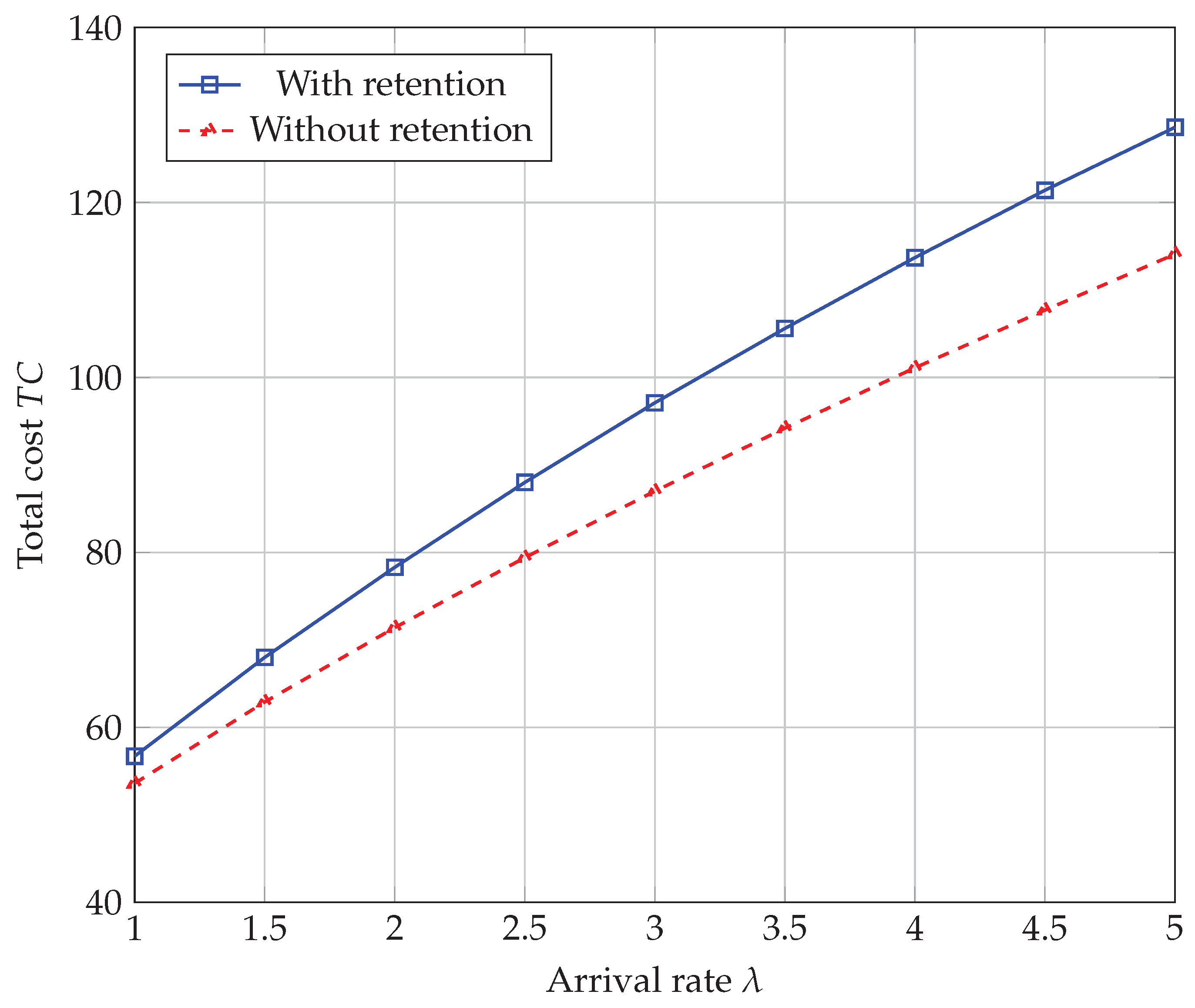
Figure 2.
Total profit versus individual retrial rate (linear vs constant retrial policy). Interpretation: Profit increases with because faster retrials reduce orbit congestion. The linear policy (blue curve) consistently outperforms the constant policy (red curve), since it accelerates retrials when the orbit is large, reducing abandonment.
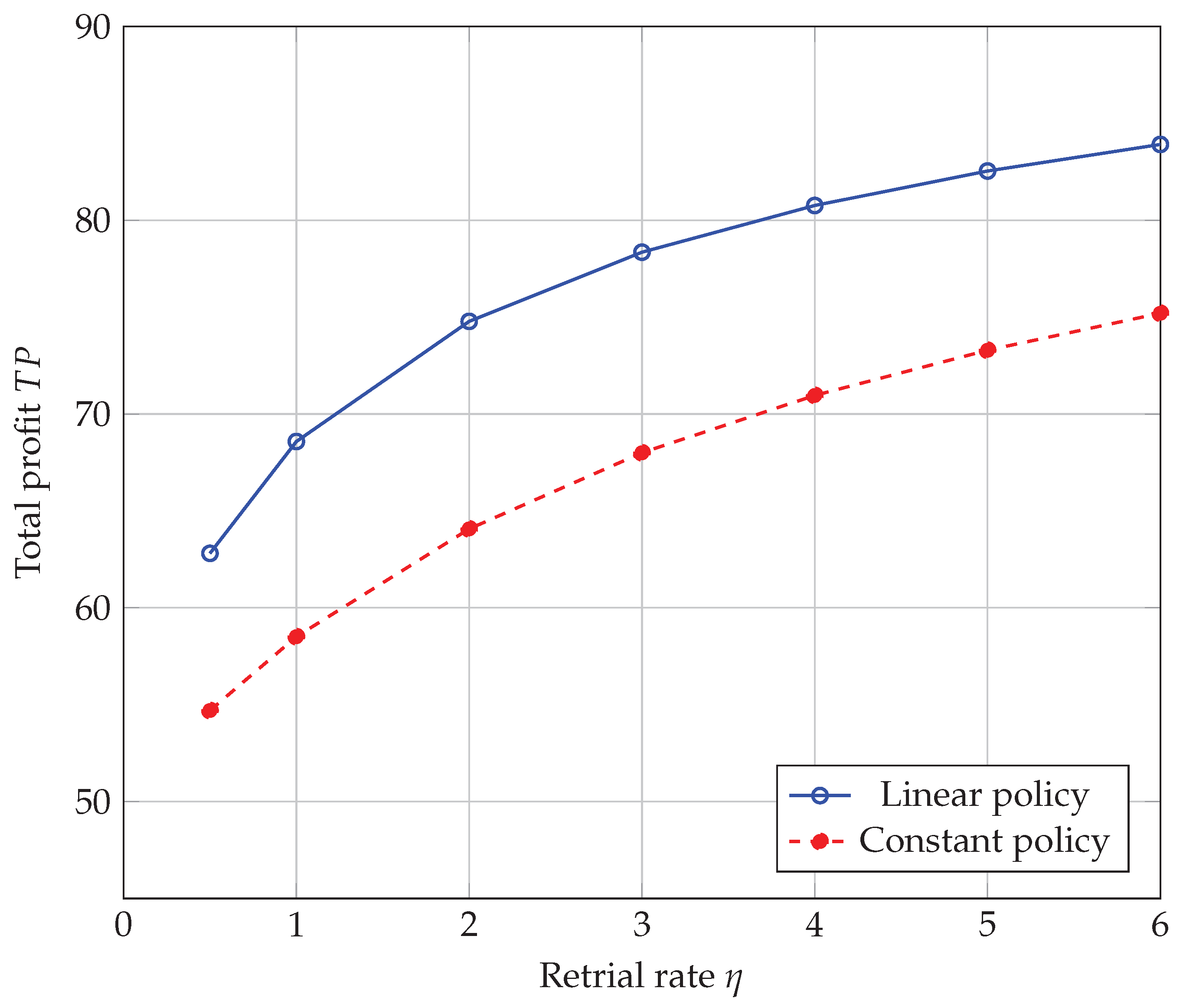
Figure 3.
Effect of retrial rate on performance measures (, , ). Interpretation: Increasing raises server busy probability , since faster retrials keep the server occupied more often, while falls as the orbit clears faster. (blocking) rises with : a faster-draining orbit frees capacity that is then filled by more accepted arrivals, which in turn raises the busy-server balking component of . This highlights a genuine trade-off between faster retrials and higher effective load on the server.
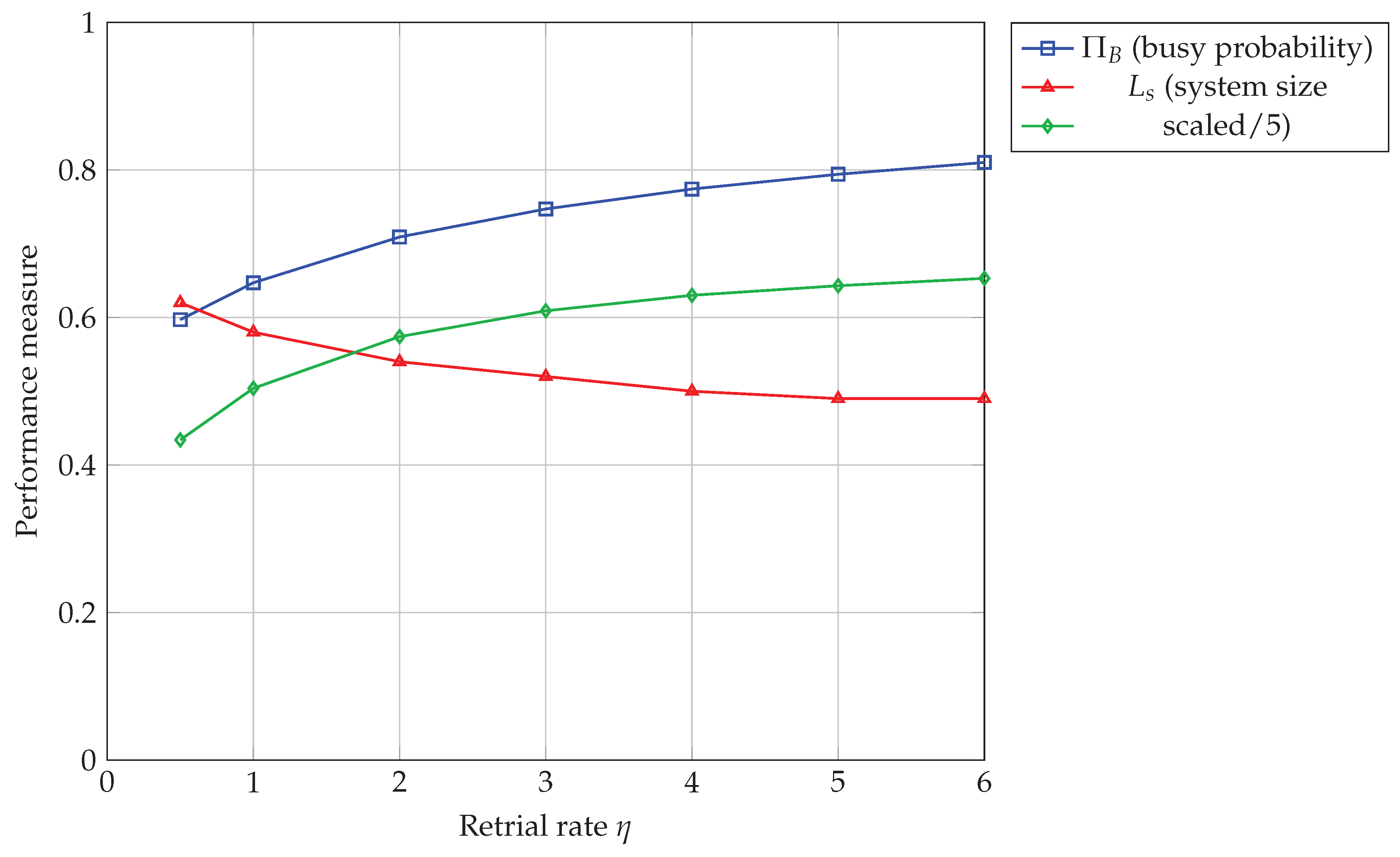
Figure 4.
Effect of impatience rate on performance measures. Interpretation: A higher makes customers more impatient, substantially increasing both the reneging rate and the retention rate (since more clock-rings occur overall), while server busy probability stays nearly flat, since accepted-arrival throughput is largely capacity- rather than impatience-limited at these parameter values.
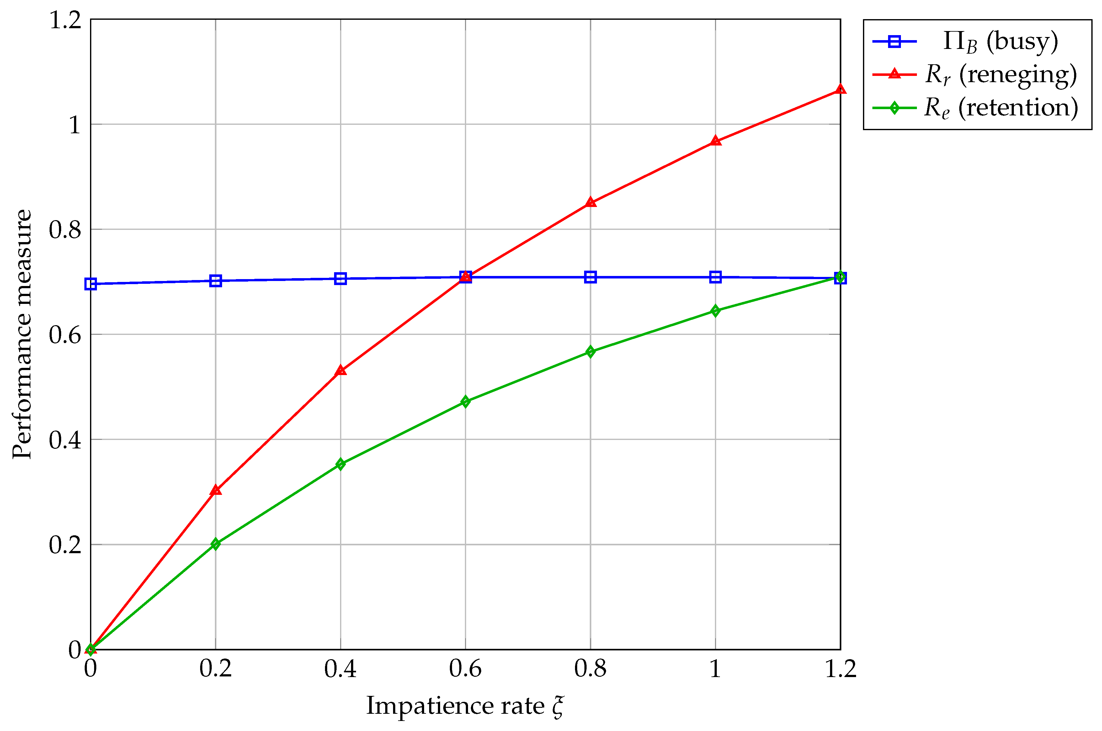
Figure 5.
Effect of feedback probability on performance measures. Interpretation: As increases, more customers re-enter the orbit after service, which increases mean system size sharply (from 2.13 to 4.34 over the range shown). Busy probability stays essentially flat, and blocking remains negligible until exceeds about , after which it rises slightly as the larger recirculating population begins to approach the finite capacity N. This confirms that feedback amplifies internal congestion well before it visibly affects external blocking.
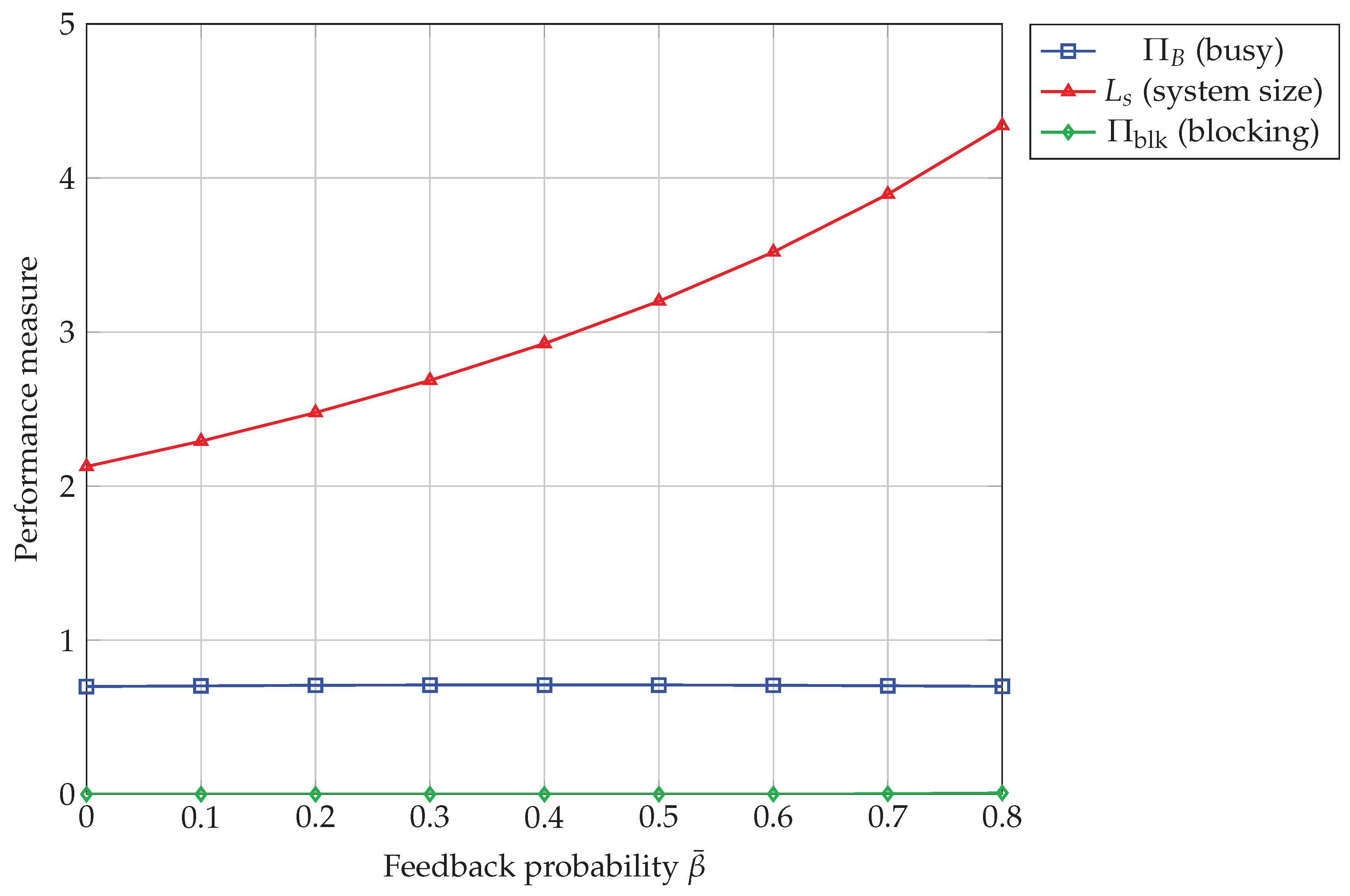
Table 1.
Transitions and rates (“−” denotes an arrival-epoch transition, which resets U).
| From | Event | Rate | To |
| , | successful retrial | ||
| , | reneging | ||
| , | vacation ends | ||
| vacation ends | (restart) | ||
| completion, departure | |||
| completion, feedback | |||
| vacation ends | |||
| , | reneging | ||
| , | completion, departure | ||
| completion, departure | |||
| completion, feedback | |||
| , | reneging | ||
| successful retrial | |||
| , | reneging | ||
| reneging (system empties) | |||
| , | arrival starts service | − | |
| arrival blocked | − | ||
| , | arrival starts service | − | |
| arrival blocked | − | ||
| , | arrival joins orbit / balks | − | w.p. / |
| arrival blocked | − | ||
| , | arrival joins orbit / balks | − | w.p. / |
| arrival blocked | − |
Table 3.
Summary of the performance measures.
| Measure | Defined in | Meaning |
| (13) | time fractions in the four server modes | |
| (14) | idle / busy-vacation / busy-normal fractions | |
| (15) | probability that an arrival is blocked | |
| (16) | loss rate; effective arrival rate | |
| (17)–(18) | mean orbit size; mean system contents | |
| (19) | successful-retrial rate | |
| (20) | reneging rate; retention rate | |
| (21) | service completion rates | |
| (22) | throughput; feedback rate | |
| (23) | mean time in orbit per orbit visit | |
| (24) | mean sojourn per accepted primary customer | |
| (25) | mean sojourn per service visit |
Table 4.
Baseline parameters.
| Parameter | Description | Value |
| mean arrival rate | 3.0 | |
| N | capacity | 8 |
| normal service rate | ||
| vacation service rate | ||
| vacation rate | 4.2 | |
| individual retrial rate | 2.0 | |
| impatience rate | 0.6 | |
| reneging probability | 0.6 | |
| departure probability | 0.7 | |
| join probability |
Table 5.
Cost parameters.
| Parameter | Description | Value |
| idle server (either mode) | 5 | |
| busy server in vacation | 7 | |
| busy server, normal | 10 | |
| holding cost per customer in system | 10 | |
| orbit-specific cost per orbiting customer | 4 | |
| cost per balked/blocked customer | 4 | |
| cost per reneged customer | 4 | |
| cost per retention event | 8 | |
| cost per service completion | 10 | |
| cost per feedback event | 5 | |
| cost per unit of provisioned capacity N | 3 | |
| R | revenue per served customer | 100 |
Table 6.
Validation of Algorithm 1 against an independent discrete-event simulation.
| Measure | Analytical (Algorithm 1) | Simulation (DES) | Relative difference |
| (idle, either mode) | 0.3206 | 0.3194 | 0.37% |
| (busy, vacation) | 0.0205 | 0.0204 | 0.49% |
| (busy, normal) | 0.6589 | 0.6602 | 0.20% |
| 2.5757 | 2.5764 | 0.03% | |
| 0.6827 | 0.6835 | 0.12% | |
| 1.5995 | 1.5971 | 0.15% |
Note: all six measures agree to within between the two independently implemented methods, providing strong evidence of the correctness of Algorithm 1. An earlier attempt to validate against the degenerate limit of [19] could not be completed, because that comparison would require the original implementation code of [19], which was not available; Proposition 2 is retained as a theoretical result (with proof sketch) but is not used here as a numerical validation anchor.
Table 7.
Effect of inter-arrival distributions.
| Distribution | ||||
| D | 0.7086 | 2.6860 | 0.5742 | 0.7075 |
| 0.6904 | 2.6486 | 0.6251 | 0.6994 | |
| 0.5862 | 2.4137 | 0.8580 | 0.6492 |
Note: decreases from D to despite having higher inter-arrival variance; this is consistent with a finite-buffer effect (higher blocking under admits fewer customers in the first place), not an inconsistency – confirmed by the monotone increase of across D, , .
Table 8.
Effect of retention probability .
| 0.2 | 0.8503 | 0.2126 | 91.52 | 70.15 |
| 0.4 | 0.7075 | 0.4717 | 97.05 | 74.78 |
| 0.6 | 0.5297 | 0.7945 | 103.95 | 80.47 |
| 0.8 | 0.3019 | 1.2075 | 112.77 | 87.64 |
Note: both and now increase with (higher retention costs more to operate, via and larger , but generates more revenue through higher throughput, so profit still rises). See the corresponding correction to Figure 1’s interpretation below.
Table 9.
Optimal solutions from PSO.
| Scenario | ||||
| Baseline (D) | 7 | 15.0 | 75.47 | 92.57 |
| Baseline () | 7 | 15.0 | 71.99 | 91.52 |
| Baseline () | 8 | 15.0 | 58.71 | 90.95 |
| High retention | 8 | 15.0 | 87.68 | 112.77 |
| Low retention | 6 | 15.0 | 71.52 | 82.83 |
| High feedback | 5 | 15.0 | 13.38 | 94.02 |
| Low feedback | 7 | 15.0 | 105.77 | 85.36 |
Note: pins at the upper search bound (15.0) in every scenario because the marginal benefit of a faster vacation-end rate saturates quickly (verified: vs. vs. differ by in at fixed N); this is a flat optimum, not a runaway one. is finite and interior because of the capacity cost in Section 5. The scenario “High feedback” () yields a markedly low because most completions do not result in permanent departure, sharply reducing effective throughput τ relative to holding costs.
Table 10.
Comparison of metaheuristics (30 independent runs each).
| Algorithm | Avg. time (s) | Best (mean ± std) | Avg. evaluations |
| PSO | 1275 | ||
| GA | 1230 | ||
| SA | 801 |
Note: PSO and GA converge to the same optimum with zero variance across all 30 runs; SA shows a small residual variance (, about of ) due to its single-trajectory stochastic acceptance rule. All three require comparable numbers of cost-function evaluations (each an solve of Algorithm 1, Section 3), consistent with the low dimensionality (2 decision variables, N and ϕ) of this optimization problem. Given this consistency, the choice among PSO/GA/SA here is a matter of implementation convenience rather than solution quality.
Table 11.
Robustness: cost variation, all cost parameters (baseline ).
| Parameter | ||||
| Sensitivity | Sensitivity | |||
| 0.018 | 0.018 | |||
| 0.000 | 0.000 | |||
| 0.095 | 0.095 | |||
| 0.340 | 0.346 | |||
| 0.100 | 0.100 | |||
| 0.034 | 0.034 | |||
| 0.036 | 0.036 | |||
| 0.048 | 0.048 | |||
| 0.222 | 0.223 | |||
| 0.048 | 0.048 | |||
| 0.245 | 0.281 | |||
Note: ranked by sensitivity, (holding cost) dominates, followed by (capacity cost), (service completion), and /; the remaining six parameters () each shift by under . Only , , and shift the optimal capacity itself (by one unit); all other parameters leave unchanged, affecting profit at the margin without altering the capacity decision.
Disclaimer/Publisher’s Note: The statements, opinions and data contained in all publications are solely those of the individual author(s) and contributor(s) and not of MDPI and/or the editor(s). MDPI and/or the editor(s) disclaim responsibility for any injury to people or property resulting from any ideas, methods, instructions or products referred to in the content. |
© 2026 by the authors. Licensee MDPI, Basel, Switzerland. This article is an open access article distributed under the terms and conditions of the Creative Commons Attribution (CC BY) license (http://creativecommons.org/licenses/by/4.0/).
Copyright: This open access article is published under a Creative Commons CC BY 4.0 license, which permit the free download, distribution, and reuse, provided that the author and preprint are cited in any reuse.