

Submitted:
24 September 2026
Posted:
28 September 2026
You are already at the latest version
Abstract
The paper proposes, implements, and tests a neural-network method based on orthogonal Laguerre polynomials for the numerical solution of the Cauchy problem for a singular nonlinear Lane--Emden equation with a variable-order fractional derivative. Such equations rarely admit analytical solutions, while classical finite-difference schemes struggle with the singularity near zero and the nonlocal character of the fractional derivative. The approximate solution is expanded in modified Laguerre polynomials shifted to the initial point, so the Cauchy initial conditions are satisfied exactly. The network has one trainable linear layer; nonlinearity is provided by the polynomial basis. The weights are found by minimizing a loss function containing the equation residual at collocation points, a weight factor improving accuracy near the singularity, and regularization limiting weight growth. Training uses Adam with an adaptive learning-rate scheduler and early stopping. Implementation is in Python with PyTorch. A vectorized tensor version accelerates computations by about thirty times compared with the loop version. On test problems with known solutions, the maximum absolute error reaches about five ten-thousandths; for a numerical reference, about five thousandths; in a stress test, about three hundredths. It is promising for singular variable-order fractional differential equations and can be parallelized on central and graphics processors.
Keywords:
Laguerre polynomials
; Gerasimov–Caputo variable-order fractional derivative
; Lane–Emden equation
; neural network
; hyperparameters
; loss function
; parallelization algorithms
1. Introduction
Modeling physical processes using differential equations often encounters limitations of the classical mathematical apparatus. In recent decades, there has been increased interest in using fractional calculus to describe systems with memory and self-similarity effects [1,2]. Unlike classical integer-order derivatives, fractional operators allow one to take into account hereditary properties and nonlocal interactions, which makes them a powerful tool for modeling a wide range of phenomena—from viscoelasticity to anomalous diffusion to spread of viruses [3,4,5,6,7]. A special place among them is occupied by variable-order operators, where the exponent of the fractional derivative is itself a function of the spatial or temporal coordinate. Such operators provide a more flexible description of systems whose rheological or diffusive properties change depending on the state or position in space [8,9,10]. One of the actively developing directions is the application of fractional calculus to problems of mathematical physics and astrophysics.
One of the important models of mathematical physics is the Lane–Emden equation [11,12,13,14], which describes the equilibrium of spherical gas clouds in stellar astrophysics. The Lane–Emden equation arises in the study of polytropic stars, the density distribution in isothermal gas spheres, and in the theory of gravitational equilibrium [15]. The introduction of a fractional derivative into this equation allows one to take into account nonlocal properties of gravitational interaction and complex thermodynamic processes, which makes the model more adequate for describing real astrophysical objects. In recent years, a number of numerical and approximate methods have been proposed for solving fractional Lane–Emden equations, including variational-iteration methods [16], spectral methods based on Legendre polynomials [17], collocation methods with wavelets [18], and other approaches [19,20]. However, most of these works consider either an integer order of the derivative or a constant fractional order, which limits their applicability to problems with variable memory.
The analytical solution of the Cauchy problem for the fractional singular nonlinear Lane–Emden differential equation exists only in particular cases (for example, for an integer exponent), which necessitates the development of efficient numerical methods [21]. Traditional approaches, such as finite-difference schemes, encounter difficulties due to the singularity of the solution near zero and the nonlocal nature of the fractional derivative. This requires the construction of special grids and leads to an increase in computational costs. In the case of a variable order of the fractional derivative, the situation becomes even more complicated, since the kernel of the fractional operator depends on the coordinate, and classical difference schemes require adaptation to each value of the exponent [22,23,24,25,26]. The problem of increasing computational costs in the numerical solution of fractional differential equations of both constant and variable order can be partially solved by parallelization, implementing both CPU versions of such algorithms and hybrid CPU-GPU analogues [27]. Accelerating computations is important when solving coefficient inverse problems for equations with fractional derivatives [28]. However, if such a numerical method has an unavoidable sequential part, the parallelization efficiency may be low.
In parallel with the development of fractional calculus, there is a rapid development of machine-learning methods. Neural-network approaches to solving differential equations (Physics-Informed Neural Networks, PINNs) have shown their effectiveness for a wide class of problems [29,30,31]. They allow one to obtain an approximate solution in analytical form without requiring grid construction and easily adapt to various types of equations and boundary conditions [32]. PINNs are successfully applied in deformable solid mechanics, heat-transfer problems, aerodynamics, and other fields [33,34]. Among the most recent developments in this direction, we note the VooPINN architecture [35]—a physics-informed neural network with a variable-order operator designed for forward and inverse problems of time-fractional partial differential equations. VooPINN demonstrates that variable-order fractional operators can be embedded directly into a neural-network framework, but it relies on a deep multilayer architecture and does not address singular ordinary differential equations with a variable-order fractional derivative, which is the subject of the present work. However, classical neural-network architectures with multilayer perceptrons are not always optimal for problems with singularities or a specific domain of definition. In addition, training deep networks requires significant computational resources and can be unstable in the presence of singularities in the solution.
In this paper, we propose a combined approach that uses the advantages of both orthogonal polynomials and neural-network optimization methods. We develop a neural-network method (LaNN—Laguerre Neural Network), where orthogonal Laguerre polynomials act as activation functions [36,37,38,39], and the basis functions are shifted to the point , which ensures exact satisfaction of the initial conditions of the Cauchy problem at . This choice is not accidental: Laguerre polynomials are defined on a semi-infinite interval and form a complete orthogonal basis, which makes them an ideal tool for expanding the solution of the Cauchy problem [38]. Note that neural-network methods based on Laguerre polynomials have already been applied to solve ordinary differential equations [36], as well as equations of the Lane–Emden–Fowler type [40]. However, these works do not consider variable-order fractional derivatives and do not use basis shifting for exact satisfaction of the initial conditions at . Unlike classical physics-informed neural networks (PINNs), which require a deep architecture, the proposed method is a network with a single “weight” layer, which simplifies the training process and interpretation of the results. The single-layer structure and the absence of separate nonlinear activations are a consequence of the fact that the Laguerre basis already provides the necessary nonlinearity. Close in spirit approaches based on wavelet neural networks also demonstrate effectiveness for fractional singular models [41], but the use of Laguerre polynomials provides a more natural representation of the solution on a semi-infinite interval and automatic satisfaction of the initial conditions. It is also worth noting a recent work [42], in which a Laguerre neural network optimized by a genetic algorithm was applied to fractal-fractional Bagley–Torvik equations. That study confirms the efficiency of the Laguerre basis for nonlocal fractional models, but it does not consider variable-order fractional derivatives, singular Lane–Emden-type nonlinearities, or exact satisfaction of Cauchy initial conditions via a shifted basis—the features that distinguish the present LaNN method.
The aim of this work is to develop, programmatically implement, and test a neural-network method based on orthogonal Laguerre polynomials with basis shifting for the numerical solution of the Cauchy problem for a fractional Lane–Emden differential equation of variable order. According to the results obtained in [36], among single-layer polynomial networks, LaNN occupies an intermediate position: it is more accurate than a network based on Chebyshev polynomials and faster than a network based on Legendre polynomials. For the class of singular fractional problems under consideration, where a combination of acceptable accuracy and computational efficiency is important, such a compromise seems justified. In addition, unlike ChNN, the Laguerre basis is defined on a half-axis, which agrees better with the nonlocality of the fractional operator. The paper describes the architecture of the LaNN network, the training algorithm based on the Adam method, and the loss function taking into account the equation residual, and provides a software implementation in the Python programming language, including the possibility of parallelization. The influence of the variable order of the fractional derivative on the complexity of the neural network is analyzed.
The paper is organized as follows. In the first section, preliminary information about orthogonal Laguerre polynomials and variable-order fractional calculus is presented. In the second section, the statement of the Cauchy problem for the fractional Lane–Emden equation is formulated. In the third section, the architecture of the LaNN network with a shifted basis, the loss function, and the training algorithm are described. In the fourth section, the software implementation of the method is considered, including vectorized and loop variants of computations. In the fifth section, the results of computational experiments are presented, and the accuracy, stability, and computational efficiency of the proposed approach are analyzed. In the conclusion, the main results are summarized and directions for further work are discussed.
2. Preliminary Information
Let us introduce some preliminary information that we will rely on in this paper.
2.1. Orthogonal Laguerre Polynomials
Laguerre polynomials are classical orthogonal polynomials widely used in mathematics, physics, and engineering. They are solutions of the Laguerre differential equation and form a complete orthogonal system on a semi-infinite interval [37,38].
Definition 1. Laguerre polynomials, denoted as , are defined as solutions of the second-order linear ordinary differential equation (Laguerre equation) [38]:
where n is a nonnegative integer. They can be defined through the Rodrigues formula [38], which is useful for their generation:
and also represented as a closed sum [38]:
Main properties [38].
1. Orthogonality and completeness. A key property of Laguerre polynomials is their orthogonality on the interval with weight function [38]:
as well as completeness, which means that any function with finite norm can be represented as a convergent series in Laguerre polynomials. These properties make them very useful for expanding functions into series.
2. Recurrence relations. Laguerre polynomials satisfy several recurrence relations that simplify their computation [38]:
2.2. Elements of Fractional Calculus
Fractional calculus can be studied in more detail in the monographs [1,2]. We will focus on some definitions and properties of Riemann–Liouville and Gerasimov–Caputo variable-order fractional derivatives [19,20,21,22,23,24,25].
Definition 2. Let the function be integrable on the interval , and let the function be sign-positive. Then the Riemann–Liouville fractional integral of order is defined as follows:
where is the Euler gamma function.
Definition 3. Let m be an integer such that . Then the Riemann–Liouville fractional derivative of order is defined as follows:
where is the ordinary integer-order derivative of order m.
Definition 4. The Gerasimov–Caputo fractional derivative of order is defined as follows:
where is the ordinary integer-order derivative of order m.
Note an important property of the fractional derivative (2):
From property (3) it follows that for . Therefore, in various applications, the Gerasimov–Caputo fractional derivative is usually chosen, since classical initial conditions are specified for it, and its derivative of a constant gives zero.
Remark on the relation between the Riemann–Liouville and Gerasimov–Caputo derivatives. The well-known relation
is valid for a constant order . In the case of a variable order , it does not hold in general, since enters both the kernel and the gamma function, and the outer derivative also acts on . Therefore, in this paper we use definition (2) directly and rely on property (3), which remains valid for a variable order as well, since is constant with respect to the integration variable .
3. Problem Statement
We consider the Cauchy problem for the fractional Lane–Emden equation:
where , the Gerasimov–Caputo variable-order fractional derivative , has the form according to (2):
Note that in the case when , , we obtain the Cauchy problem for the classical Lane–Emden equation with exponential nonlinearity [3,4,8,9].
Remark on the lower limit of the fractional derivative. When stating the Cauchy problem for an equation with a fractional derivative , the lower limit of the fractional operator plays an important role. If the initial conditions are specified at a point , then the operator for uses the values of on the entire interval , including the segment , which is not described by the initial conditions. In this case, the Cauchy problem at for an operator with lower limit 0 is not well-posed without specifying the prehistory of the solution on .
In this paper, two scenarios are considered.
First scenario (original problem). In Section 6, for , we set . The initial conditions are specified at , and the lower limit of the fractional derivative coincides with the point where the initial conditions are specified. There is no prehistory, and the statement is well-posed.
Second scenario (test problem with a known exact solution). When verifying the method, the manufactured-solution technique is used: the equation is considered on the entire interval with a known exact solution that satisfies the operator . The initial conditions at are taken from this exact solution, so that the prehistory on is implicitly specified by itself. This is a standard technique for testing numerical methods, and no contradiction with the statement arises.
It should be emphasized that for the neural-network approximation , coincidence with on is not guaranteed: the basis functions are defined for all through the analytic continuation , but the equation on is not included in the loss function. Therefore, examples with in Section 6 should be interpreted precisely as manufactured-solution tests, where the prehistory is known from the exact solution, and not as a demonstration of a well-posed Cauchy problem with arbitrary . Practical problems with and unknown prehistory require a transition to the operator (7); the modification of the method in this direction was not carried out and is a subject of further work.
For practical problems in which the initial conditions are specified at a point and the prehistory on is unknown, one should use the fractional derivative with lower limit :
Such an operator takes into account only the part of the solution that is determined by the initial conditions at and leads to a well-posed Cauchy problem. The transition from to in the proposed LaNN method reduces to replacing with in the formulas for the fractional derivative of the basis functions. This can be a subject of a separate study; in this paper, the main emphasis is on the case (original problem) and on the verification of the method using the manufactured solution (test examples).
The classical Lane–Emden equation with exponential nonlinearity arises in the description of hydrostatic equilibrium of spherically symmetric polytropic stars, isothermal gas spheres, and gravitationally bound clouds. In this context, x is a dimensionless radial coordinate, and is a dimensionless Emden function, which can be interpreted as the logarithm of density, temperature, or as a dimensionless gravitational potential. The term reflects the spherical geometry of the Laplace operator: it appears in the transition from Cartesian coordinates to radially symmetric ones. The nonlinear term models an effective source/self-action that depends exponentially on the state of the medium. If y is interpreted as the logarithm of dimensionless density, then is proportional to density, and is a weaker nonlinear factor that may correspond, for example, to heat release, reaction, or nonlinear coupling with the gravitational field.
The Gerasimov–Caputo variable-order fractional derivative in the model equation (5) generalizes the second derivative and introduces the effect of spatial nonlocality into the model. Unlike the classical second derivative, which is determined only by the local behavior of the function, the fractional operator takes into account the prehistory or distribution of the solution on the entire interval . The variable order means that the degree of nonlocality changes with radius: in internal regions and on the periphery, the memory contribution may be different. This allows one to describe media whose rheological, thermal, or gravitational properties depend on the local state. The right-hand side plays the role of an effective external source or sink: it can be a mass distribution, energy release, or an external field. The initial conditions , specify the value of the function and its gradient at the starting radius.
4. LaNN Architecture and Its Description
The neural-network method allows one to obtain the solution of problem (5) in the form:
where are modified Laguerre polynomials with a shift to the point that satisfy the initial conditions (5):
are binomial coefficients, N is the order of the Laguerre polynomial, and are weight coefficients that are refined during training. The basis shift to the point ensures exact satisfaction of the initial conditions of the Cauchy problem for any , which is fundamentally important for singular problems where may be different from zero.
It should be emphasized that the basis shift to the point ensures exact satisfaction of the initial conditions but does not change the lower limit of the fractional operator. In this paper, the fractional derivative is taken with the operator with lower limit 0. This corresponds either to the case (original problem) or to the case when the solution on is known and taken into account in the right-hand side (test examples with manufactured solution). For practical problems with and unknown prehistory, one should use the operator ; the corresponding formulas are obtained by replacing with .
Training proceeds as follows. A training sample of fixed size M is chosen from . The points of this sample are called collocation points.
Remark 1. Collocation points can be chosen in different ways, for example, uniformly on the entire interval or subject to some distribution, for example, logarithmic or Chebyshev.
Then, at the chosen collocation points, the residual between the left-hand side of equation (5) with account for (8) and its right-hand side is calculated:
Here, the Gerasimov–Caputo fractional derivative of the shifted basis is calculated taking into account the binomial expansion:
Note that the linear terms give a zero contribution to the Gerasimov–Caputo fractional derivative of order , since for .
Then we form the loss function as the normalized weighted mean-square value of the residual at the collocation points (9) with the addition of -regularization of the weights of solution (8):
where is the regularization parameter, are the weights of the collocation points, and is the mean value.
Remark 2. It should be noted that the weight coefficients for the collocation points can be chosen to improve accuracy in the region of small values, where the solution has a singularity.
Remark 3. -regularization allows one to avoid overfitting and excessively large weight coefficients of solution (8). The neural network can adapt to noise or specific features of a particular set of collocation points, which leads to nonsmooth or nonphysical solutions. -regularization limits the growth of weight coefficients, promoting a smoother approximation. In addition, with a large number of parameters (high polynomial degree), the weight coefficients can become very large, causing numerical instability (Runge’s phenomenon). Regularization mitigates this effect. The loss function shows how strongly the equation is violated at the collocation points (10). The smaller the loss, the better the network “knows” the solution. To achieve this, it is necessary to reduce this loss by updating (choosing) the weight coefficients at each iteration.
Remark 4. The process of constructing the loss function (10) is called the forward pass. It forms a computational graph that stores the sequence of operations and is necessary for the subsequent calculation of derivatives (gradients).
The weights are updated in accordance with the Adam (Adaptive Moment Estimation) algorithm from the family of gradient descent methods.
The formulas for the weights at iteration k are as follows:
Remark 5. It should be noted that usually the gradients (11) are calculated using the backpropagation algorithm. The backward pass through the computational graph from the loss function node to the model weights is performed using the chain rule. Therefore, the process of constructing gradients is called the backward pass.
2. Biased estimates of the first and second moments:
the parameter values , are taken by default.
3. Bias correction:
4. Weight update:
where is the initial learning rate, is a small constant to avoid division by zero (usually ).
One training cycle (epoch) consists of one forward and one backward pass over all collocation points, as well as an optimizer step (Adam), i.e., updating the weights to reduce the loss function. For each training epoch, after updating the weights, it is necessary to zero the gradients to prevent their accumulation.
As a result, after a given number of training epochs, solution (8) is output with an optimal set of weight coefficients . The architecture of the network with a shifted basis is shown in Figure 1.
Here, the input x is transformed into the shifted variable . Then the basis functions are multiplied by the trainable weights . The term ensures exact satisfaction of the initial conditions. The results are summed and fed to the output .
5. Implementation of the LaNN Architecture
The LaNN neural-network architecture was implemented in the Python programming language [43] using the PyTorch library [44].
The main implementation stages are as follows:
1. Initialization of parameters—input of the derivative order , the polynomial degree N, the number of collocation points, training and regularization parameters, choice of the weight function, early-stopping settings, and the coordinate of the initial point . The early-stopping condition can be, for example, the absence of improvement by at least 0.1% from the best value over a number of epochs, after which training stops. This can save computational time. The regularization parameter is by default.
2. Construction of the neural-network model—the LaguerreNN class, which implements the approximation of the solution using shifted Laguerre polynomials and automatically takes into account the initial conditions (5) at the point . The LaguerreNN class implements the fractional derivative with the operator . The x0 parameter specifies the basis shift point and the point where the initial conditions are specified. For x0 = 0, the statement of the Cauchy problem is well-posed without additional assumptions. For x0 > 0, the method should be applied either in the manufactured-solution mode (when the prehistory is known from the exact solution) or after replacing the operator with .
3. Formation of the training set—a set of points on the interval. Three distributions are provided: uniform using torch.linspace; logarithmic using torch.logspace, which gives more points near zero, where the solution and its derivative change rapidly; and the Chebyshev distribution, which gives clustering of points near the boundaries of the interval. The number of points is specified by the user (by default 10,000).
4. Training of the model—minimization of the special loss function (10), including the residual (9), the weight function, and regularization. The weight function allows one to focus on regions with large errors (for example, near zero). The user can choose an arbitrary expression, for example . If the user does not choose weights, this is equivalent to the uniform case, where . Before use, the weights are normalized so that their mean value equals 1 (this does not affect the optimum but stabilizes the gradient scale).
5. Optimizer—Adam is used with a given initial learning rate. To automatically reduce the step on the loss-function plateau, the ReduceLROnPlateau scheduler is used with a reduction factor of 0.5 and a patience of 500 epochs. The scheduler controls the learning rate , which can decrease if the loss function stops decreasing over a given number of epochs, i.e., the learning rate is adaptive.
6. Evaluation of results—comparison with the exact solution on a test grid, output of a table and graphs. The maximum and mean absolute errors are calculated, and a comparison table at the nodes x is constructed. Visualization includes four graphs: comparison of the exact and approximate solutions; error on a logarithmic scale; loss function; and the function .
7. Computation modes. When solving the Cauchy problem (5) for fractional differential equations using the neural-network approach, the computational costs can be significant, especially when using a large number of collocation points (up to 200,000), high polynomial degrees (up to 30), and a large number of training epochs (up to 10,000). To accelerate computations in the developed method, parallelization algorithms implemented using the PyTorch library and the hardware capabilities of modern computing systems are used.
Two variants of the forward pass of the network are implemented:
- Loop (forward_loop): sequential summation over indices using Python loops. A slow mode, but more understandable.
- Vectorized (forward_vectorized): all operations are performed using PyTorch tensor operations on the CPU. At the algorithmic level, the key technique here is replacing loops over polynomial degrees (from 0 to degree) with tensor operations. In the forward_vectorized variant, all basis functions, their derivatives, and fractional derivatives are calculated using broadcasting and matrix multiplications. This allows efficient use of CPU SIMD instructions. As shown in Section 5, the vectorized version works on average 30 times faster than the loop version, and the use of vectorization does not require changing the network architecture and is completely equivalent in output values.
Some computational aspects: all tensors and the model are moved to the device specified in the device variable (CPU); for numerical stability, the gamma function is calculated using torch.lgamma and exponentiation to avoid overflow for large argument values; the polynomial degree is limited to 30 to prevent instability and overflow.
6. Simulation Results
For further calculations, a personal computer with the following characteristics was used: operating system Windows 11; processor 12th Gen Intel(R) Core(TM) i9-12900KF; logical cores: 24; physical cores: 16; current frequency: 3200 MHz; maximum frequency: 3200 MHz; current CPU load: 2.3%; RAM: 128 GB; graphics card NVIDIA GeForce RTX 4060 Ti. The calculations were performed without using CPU multithreading or CUDA cores.
Remark 6. It should be noted that the selection of hyperparameters (number of collocation points, number of epochs, and regularization coefficient) was carried out manually based on a series of preliminary experiments. The criteria were: training stability, absence of solution oscillations, absence of overfitting, accuracy on the test grid, and acceptable computation time. The absence of systematic automatic hyperparameter selection is a limitation of the work. A more rigorous approach, for example Bayesian optimization or grid search taking into account training time, can be implemented in the future.
Remark 7. (Remark on the statement of initial conditions.) In all examples of this section where the right-hand side (Examples 3 and 4), the initial conditions are specified at the point :
The computational domain begins at , which allows avoiding the singularity of the term at zero. The shift of the Laguerre basis is performed to the point , which automatically ensures satisfaction of the initial conditions. In test examples 1 and 2, the initial conditions are specified at the point and are taken from the exact solution; the prehistory on is known in this case, and the statement of the Cauchy problem is well-posed.
Remark 8. (On collocation points and the interval .) In all examples, the collocation points are chosen on the interval , where . The contribution of the segment to the fractional derivative is taken into account analytically through the global LaNN ansatz: the basis functions are defined for all , and their fractional derivative is calculated by the formula given in Section 3. The initial conditions at zero fix the linear terms. At the same time, the equation on the interval is not included in the loss function, and the behavior of the solution there is controlled only by the analytic continuation of the ansatz. This may introduce additional error that decreases with decreasing . The study of the sensitivity of the method to the choice of was not carried out in this paper and is a direction for further research.
6.1. Test Example 1
Thanks to the basis shift to the point , the initial conditions are satisfied exactly:
The solution of problem (12) is the function
The hyperparameters for LaNN training are given in Table 1.
The collocation points are chosen uniformly distributed on . Training was completed in 13.42 s, best Loss: . The LaNN training results are given in Table 2.
At the table nodes, the error varies from at to at ; at , the error is . The largest absolute errors are concentrated in the middle and right parts of the interval. Near zero, the absolute error is small due to the smallness of the solution itself, but the relative error there can be noticeable. This is expected for a singular fractional Lane–Emden equation with the point and variable order . The weight shifts the emphasis to the right part. Note that the initial conditions at are satisfied exactly due to the basis shift.
It can be seen (Table 3) that MAE and RMSE are close, which indicates the absence of large outliers. Figure 2 shows graphs of the exact (13) and neural-network solutions, the loss function, and the absolute error.
Note that Loss decreases from to . After about 8000 epochs, the improvement slows down, so early stopping is possible here to save time.
To verify the stability of the calculations with respect to the initialization of the LaNN weights for Example 1, a computational experiment with 10 independent training runs was conducted. The reproducibility parameters of the computational experiment are given in Table 4.
The experiment was conducted without early stopping, so and patience are not defined. The results of the experiment are given in Table 5.
The relative spread of accuracy metrics (ME, MAE, RMSE) does not exceed 9.2%, and that of training time is 2.5% (Table 6).
The largest spread is observed for the internal metric Best Loss (11.0%), which is expected, since it reflects the optimization trajectory rather than the quality of the final solution. All 10 runs produced a correct solution without oscillations or outliers (Figure 3).
It should also be noted that a comparison was made with a neural network based on the Legendre basis under identical conditions (settings). Five independent runs (seeds) were performed, and the averaged metrics were calculated and are presented in Table 7.
The Laguerre-basis neural network demonstrated superior performance here: it outperformed the others by approximately 2.2 times in terms of BestLoss, 2.9 times in RMSE, 3.0 times in ME, and 2.5 times in MAE; regarding ±Std, the Laguerre network was more stable, showing less variation between runs; and there was virtually no difference in training time.
This example demonstrates that LaNN can yield better results than other polynomial-based neural networks.
Remark 9. Equation (12) has a singularity in the term near the boundary point ; therefore, the numerical solution obtained on the basis of LaNN can differ strongly due to large values of the derivative, which leads to a large deviation from the true solution and complicates the physical interpretation of the process. Therefore, to improve accuracy, it is necessary to cluster points near the boundary point . This can be achieved by choosing the distribution of collocation points according to the Chebyshev law.
6.2. Test Example 2 (Stress Test)
Consider the Cauchy problem (12). Choose the interval ; here , so . Also choose the weight , which will shift the emphasis to the left part of the interval under consideration, i.e., clustering of points near the singularity will occur. The values of the remaining parameters for LaNN training are taken from Table 1, and the collocation points are still uniformly distributed. The training results are given in Table 8.
We see (Table 8) that near the singularity , a significant deviation from the exact solution (13) occurs, negative values appear in the numerical solution, and the absolute error accumulates (Figure 4). We observe signs of poor conditioning of the method.
If the collocation points are chosen according to the Chebyshev law, which produces clustering of points near the boundaries of the interval , we obtain a better result (Table 9).
From Table 9, we see that the error near the boundaries is significantly lower than the error in Table 8, and all values of the numerical solution are positive. Note that the maximum error in this example reaches (at ), which is higher than in Example 1 and is explained by the greater singularity of the problem on the interval .
The LaNN training times for the vectorized version (), built on tensor operations, and the loop version (), based on classical loops, are given in Table 10. The hyperparameter values were taken from Table 1. The collocation points were chosen uniformly and according to Chebyshev.
Here one can see that the vectorized version trains on average 30 times faster than the loop version (the ratio ranges from 27.4 to 30.6). We see that the vectorized implementation in PyTorch based on tensor operations can give a speedup of about 30 times for this example. One can try to further accelerate LaNN training by implementing a parallel algorithm for CPU or GPU, but this is a topic for future research.
6.3. Test Example 3
Consider problem (5) with , , . Parameters for LaNN training: ; number of epochs 8000; initial learning rate ; -regularization coefficient ; polynomial degree ; number of collocation points , uniformly distributed on ; weights for the residual: , , .
Since in this case we do not know the exact solution of problem (5) as in Example 1, we need to find a numerical solution. For this purpose, we use an implicit nonlocal finite-difference scheme of the first order of accuracy based on the Grünwald–Letnikov approximation with the Gerasimov–Caputo correction [45]. The calculations were performed on a uniform grid with step , . The nonlinear equation at each step was solved by Newton’s method with accuracy . The scheme has the first order of approximation in h. A rigorous study of the grid convergence of the reference solution was not carried out in this paper; indirect confirmation of its suitability is its agreement with the analytical solution in test examples 1 and 2, where the exact solution is known.
The calculated data are given in Table 11.
Table 11 shows how the choice of the weight function in the loss function affects the accuracy of the LaNN neural-network solution when solving the fractional Lane–Emden equation with and variable order . The numerical solution obtained by the Grünwald–Letnikov finite-difference scheme with the Gerasimov–Caputo correction is used as a reference. The table compares three weight variants: , , . The columns are the absolute errors for the corresponding weights.
At the left boundary point , all three LaNN variants give values practically coinciding with the reference . The errors are for , for , and for . This confirms that correct account of the initial conditions , does not introduce additional error at the boundary of the computational domain.
The reference solution decreases from at to at , changing sign in the middle part of the interval. All three neural-network solutions qualitatively reproduce this behavior without giving nonphysical oscillations or outliers. The differences between the variants with different are small compared to the amplitude of the solution.
The error is mainly of order –. The most noticeable deviations are concentrated in the region –, where the errors reach . Closer to the right boundary, the errors usually decrease to . This indicates acceptable accuracy of the method for this example, where the exact analytical solution is unknown and the reference is obtained numerically. Note that the errors given in Table 11 at individual nodes (up to ) do not contradict the integral metrics , , for the case : the integral metrics were calculated on a denser test grid of 2000 points, while the table contains only 10 characteristic nodes, and in the neighborhood of – the local error may exceed the mean.
The weight gives the most uniform error distribution. For , the error varies from at to at , without sharp local spikes. In terms of integral metrics, this variant has the smallest maximum error: with and . That is, the uniform weight gives a balanced approximation.
The weight shifts the emphasis to the right but does not give an explicit gain. For , the error in the left section – turns out to be the largest among the three variants: and . At the same time, the total loss function for this variant is the highest: , and . This means that concentration on the right part of the interval does not lead to an improvement in global accuracy for this example.
The weight improves training and accuracy near the left boundary. For , the smallest value of the loss function is achieved: , which indicates faster and more stable training. Near the initial point, the error is minimal ( at ), and at a number of right points, for example , , , the error is also smaller than for the other variants. At the same time, the maximum error only slightly exceeds the value for . Thus, the weight is a successful compromise: it strengthens the left part, where the solution and its derivative change faster, and at the same time does not worsen the overall accuracy.
The choice of the weight function controls not so much the overall accuracy as the distribution of the error. The mean metrics for all three cases are close: , . This means that LaNN is stable with respect to the choice of , but the local accuracy in different parts of the interval can be purposefully redistributed. If uniform accuracy is needed, is better; if behavior near the singularity is more important, is preferable.
Consider an example with a different function .
6.4. Test Example 4
Consider problem (5) with and the same initial conditions as in Example 3: , . Parameters for LaNN training: , , the remaining parameters are taken from Example 3.
In Table 12, it can be seen that for , the neural-network solution changes sign and becomes negative. It is important to emphasize that this is not an artifact of LaNN training: the reference numerical solution behaves similarly, and the error remains small (ME , MAE , RMSE ). Consequently, the negative values reflect a property of the mathematical model itself for the chosen variable order of the fractional derivative.
The physical admissibility of negative y depends on the interpretation of the function . Since the equation contains exponential nonlinearities and , it is most natural to interpret y not as density or temperature itself but as the logarithm of dimensionless density/temperature or as a dimensionless potential. In this case, a negative y does not mean negative density or temperature: the physical quantity remains strictly positive. For example, at we have , whence ; at , , . This means that density/temperature or potential become smaller than some reference value but do not lose physical meaning.
The metrics: ME: , MAE: , RMSE: indicate the absence of outliers in the values. The numerical algorithm worked in 0.08 s.
From Figure 5, we see that the LaNN neural network copes well with finding the solution of the problem: this is visible when comparing with the numerical solution. Also, from the loss function, it can be seen that the number of epochs can be reduced to 7000, which will accelerate training.
To confirm the efficiency of the neural-network algorithm, the inference time was measured—the direct run of an already trained model with fixed weight coefficients on a test sample of 2000 points. For this purpose, 10 runs were performed for the same trained model (Table 13). The goal is to evaluate the stability of the forward-pass time.
From Table 13, it can be seen that the inference time is approximately 1.5–1.9 milliseconds per run. The spread between runs is small, which indicates the stability of the computations. The fastest execution is 1.46 ms, and the slowest is 1.87 ms. These values show that the forward pass of the network takes fractions of a second, which is quite acceptable for many practical problems.
Next, the metrics were calculated (Table 14).
The mean inference time for 2000 points is 1.66 ms, and per point it is 0.83 microseconds (Table 14). This is a very high computation speed. The standard deviation of ms confirms that the execution time varies weakly, i.e., the algorithm works predictably. The minimum and maximum are also close to the mean, which indicates the absence of outliers.
7. Conclusions
In this work, the LaNN (Laguerre Neural Network) neural-network method for the numerical solution of the Cauchy problem for the fractional Lane–Emden equation of variable order has been developed, programmatically implemented, and tested. The method is based on representing the solution as an expansion in orthogonal Laguerre polynomials with a shift to the point , which ensures exact satisfaction of the initial conditions of the Cauchy problem at . The weight coefficients are tuned during training by minimizing a special loss function that includes the residual of the differential equation and -regularization. The conducted computational experiments have shown the following.
In test examples with a known analytical solution (Examples 1 and 2), the maximum absolute error was for the interval and for the substantially singular interval with the Chebyshev distribution. In examples with a numerical reference (Examples 3 and 4), the maximum absolute error did not exceed . These values confirm the efficiency of LaNN for the class of singular fractional differential equations. The basis shift allows exact satisfaction of the initial conditions for any ; in examples with , the initial conditions were specified at , and the shift to was applied in test examples with a manufactured solution.
The uniform and Chebyshev distributions give comparable results; however, the choice of distribution can be optimized depending on the behavior of the solution. In particular, for the strongly singular interval , the Chebyshev distribution made it possible to reduce the maximum error by more than a factor of 60 compared with the uniform distribution (from to ).
The introduction of weights into the loss function allows one to control local accuracy: weights growing toward the boundary increase accuracy near the singularity. In Example 3, the weight gave the smallest value of the loss function () and the minimum error near , while the weight gave the most uniform error distribution over the interval.
A change in the exponent substantially affects the complexity of training. For , the value of the loss function turned out to be more than an order of magnitude higher than for , which indicates the need to adapt the architecture (for example, increase the polynomial degree or the number of collocation points) to preserve accuracy.
The vectorized implementation in PyTorch provides an average speedup of 30 times compared with the loop implementation and acceptable computation time (units to tens of seconds) for practical problems. The possibility of parallelization on a GPU can give a further increase in the speed of the training algorithm.
It has been shown that after training, the LaNN neural network provides fast and stable inference. This is a key advantage over traditional numerical methods, which may require re-solving the system of equations when points or parameters change. The obtained time characteristics (about 1.66 ms for 2000 points, or 0.83 s per point) confirm that the method is suitable for practical use, especially in problems where multiple evaluations of the solution at different points with fixed model parameters are required. In combination with the possibility of parallelization on a GPU, this makes LaNN a promising tool for the numerical analysis of variable-order fractional differential equations, especially in cases where classical methods encounter difficulties due to singularity or nonlocality.
The proposed LaNN implementation uses the operator . This is natural for problems with and for verification by the manufactured-solution method. For practical problems with initial conditions at a point and unknown prehistory on , a transition to the operator is required. Modification of the method in this direction seems promising and will be considered in further work.
Compared with classical finite-difference schemes, the LaNN method does not require grid construction, provides an analytical representation of the solution, and has fast inference (about 1.5–1.9 ms for 2000 points). Compared with physics-informed neural networks (PINNs), LaNN uses a single weight layer and an orthogonal Laguerre basis, which simplifies training and interpretation. Compared with spectral methods based on Legendre or Chebyshev polynomials, LaNN is naturally defined on a half-axis and agrees better with the nonlocality of the fractional operator. In contrast to the recently proposed VooPINN [?], which handles variable-order operators within a deep PINN architecture, LaNN uses a single trainable layer with an orthogonal Laguerre basis, which simplifies training and interpretation. Compared with the GA-optimized Laguerre network for fractal-fractional Bagley–Torvik equations [?], the present method additionally employs a shifted basis for exact enforcement of the Cauchy initial conditions and is adapted to the singular Lane–Emden nonlinearity. At the same time, a direct quantitative comparison of LaNN with PINNs, spectral methods, and high-order finite-difference schemes was not carried out in this paper. This is a limitation and a direction for future research.
The limitations of the work include: (a) manual selection of hyperparameters; (b) absence of a systematic study of the grid convergence of the reference solution ; (c) absence of a quantitative comparison with other numerical and neural-network methods; (d) absence of an analysis of the sensitivity of the method to the choice of for ; (e) limitation of the domain of applicability to the cases and manufactured solution for .
Further research may be aimed at adapting the method to multidimensional problems, using other orthogonal bases (Hermite, Legendre), and integrating with active-learning methods for automatic selection of collocation points, as well as improving parallel training algorithms on CPU or GPU [26]. A separate direction is the transition to the operator for practical problems with and unknown prehistory.
Author Contributions
Conceptualization, D.T. and R.P.; methodology, D.T. and R.P.; software, D.T.; validation, D.T. and R.P.; formal analysis, D.T. and R.P.; investigation, D.T. and R.P.; resources, R.P.; data curation, D.T.; writing—original draft preparation, D.T.; writing—review and editing, R.P.; visualization, D.T.; supervision, R.P.; project administration, R.P.; funding acquisition, R.P. All authors have read and agreed to the published version of the manuscript.
Funding
This work was carried out within the framework of the state assignment of IKIR FEB RAS No. 124012300245-2.
Data Availability Statement
The data presented in this study are available on request from the corresponding author.
Conflicts of Interest
The author declares no conflicts of interest.
Abbreviations
The following abbreviations are used in this manuscript:
| LaNN | Laguerre Neural Network |
| PINN | Physics-Informed Neural Network |
| GC | Gerasimov–Caputo |
| RL | Riemann–Liouville |
| GL | Grünwald–Letnikov |
| ME | Maximum Error |
| MAE | Mean Absolute Error |
| RMSE | Root-Mean-Square Error |
| CPU | Central Processing Unit |
| GPU | Graphics Processing Unit |
References
- Kilbas, A.A.; Srivastava, H.M.; Trujillo, J.J. Theory and Applications of Fractional Differential Equations; Elsevier: Amsterdam, The Netherlands, 2006. [Google Scholar]
- Nakhushev, A.M. Fractional Calculus and Its Applications; Fizmatlit: Moscow, Russia, 2003. (In Russian) [Google Scholar]
- Podlubny, I. Fractional Differential Equations; Academic Press: San Diego, CA, USA, 1999. [Google Scholar]
- Mainardi, F. Fractional Calculus and Waves in Linear Viscoelasticity; Imperial College Press: London, UK, 2010. [Google Scholar]
- Evangelista, L.R.; Lenzi, E.K. Fractional Anomalous Diffusion. In An Introduction to Anomalous Diffusion and Relaxation; Springer, 2023; pp. 189–236. [Google Scholar]
- Ukaj, N.; Hellmich, C.; Scheiner, S. Aging Epidemiology: A Hereditary Mechanics–Inspired Approach to COVID-19 Fatality Rates. J. Eng. Mech. 2024, 150. [Google Scholar] [CrossRef]
- Tverdyi, D.A.; Parovik, R.I. Fractional Riccati equation to model the dynamics of COVID-19 coronavirus infection. J. Phys. Conf. Ser. 2021, 2094, 032042. [Google Scholar] [CrossRef]
- Sun, H.; Chang, A.; Zhang, Y.; Chen, W. A Review on Variable-Order Fractional Differential Equations: Mathematical Foundations, Physical Models, Numerical Methods and Applications. Fract. Calc. Appl. Anal. 2019, 22, 27–59. [Google Scholar] [CrossRef]
- Patnaik, S.; Hollkamp, J.P.; Semperlotti, F. Applications of variable-order fractional operators: A review. Proc. R. Soc. A 2020, 476, 20190498. [Google Scholar] [CrossRef] [PubMed]
- Tverdyi, D.A.; Makarov, E.O.; Parovik, R.I. Research of Stress-Strain State of Geo-Environment by Emanation Methods on the Example of α(t)-Model of Radon Transport Bull. KRASEC Phys. Math. Sci. 2023, 44, 86–104. [Google Scholar] [CrossRef]
- Lane, J.H. Art. IX.—On the Theoretical Temperature of the Sun; under the Hypothesis of a Gaseous Mass maintaining its Volume by its Internal Heat, and depending on the Laws of Gases as known to Terrestrial Experiment. Am. J. Sci. Arts 1870, 50, 57–74. [Google Scholar] [CrossRef]
- Emden, R. Gaskugeln: Anwendungen der mechanischen Wärmetheorie auf kosmologische und meteorologische Probleme; B.G. Teubner: Leipzig, Germany, 1907. [Google Scholar]
- Chandrasekhar, S. Introduction to the Study of Stellar Structure; Dover: NY, USA, 2012; 512p. [Google Scholar]
- Parand, K.; Dehghan, M.; Rezaei, A.R.; Ghaderi, S.M. An approximation algorithm for the solution of the nonlinear Lane–Emden type equations arising in astrophysics using Hermite functions collocation method. Comput. Phys. Commun. 2010, 181, 1096–1108. [Google Scholar] [CrossRef]
- Horedt, G.P. Polytropes: Applications in Astrophysics and Related Fields; Kluwer Academic Publishers: Dordrecht, The Netherlands, 2004. [Google Scholar]
- Kannaujiya, L.N.; Verma, A.K. A note on hybrid approach of variational iteration method for a type of fractional Lane–Emden equations. Sib. J. Comput. Math. 2026, 29, 253–264. [Google Scholar]
- Izadi, M.; Baleanu, D. An effective QLM-based Legendre matrix algorithm to solve the coupled system of fractional-order Lane–Emden equations. Appl. Numer. Math. 2023, 188, 1–15. [Google Scholar] [CrossRef]
- Singh, R.; Garg, H.; Guleria, V. Haar wavelet collocation approach for Lane–Emden equations arising in mathematical physics and astrophysics. Eur. Phys. J. Plus 2019, 134, 548. [Google Scholar] [CrossRef]
- Saadatmandi, A.; Ghasemi-Nasrabady, A.; Eftekari, A. Numerical study of singular fractional Lane–Emden type equations arising in astrophysics. J. Astrophys. Astron. 2019, 40, 27. [Google Scholar] [CrossRef]
- Delkhosh, M.; Parand, K. An efficient numerical method for solving nonlinear astrophysics equations of arbitrary order. Hacet. J. Math. Stat. 2019, 48, 1601–1619. [Google Scholar] [CrossRef]
- Nagy, A.M. Non-Standard finite difference schemes for solving variable-order fractional differential equations. Differ. Equ. Dyn. Syst. 2021, 29, 623–632. [Google Scholar] [CrossRef]
- Ortigueira, M.D.; Valério, D.; Machado, J.T. Variable order fractional systems. Commun. Nonlinear Sci. Numer. Simul. 2019, 71, 231–243. [Google Scholar] [CrossRef]
- Parovik, R.I. Mathematical Model of a Wide Class Memory Oscillators. Bull. South Ural State Univ. Ser. Math. Model. Program. Comput. Softw. 2018, 11, 108–122. [Google Scholar] [CrossRef]
- Novozhenova, O.G. Life And Science of Alexey Gerasimov, One of the Pioneers of Fractional Calculus in Soviet Union. FCAA 2017, 20, 790–809. [Google Scholar] [CrossRef]
- Caputo, M.; Fabrizio, M. On the notion of fractional derivative and applications to the hysteresis phenomena. Meccanica 2017, 52, 3043–3052. [Google Scholar] [CrossRef]
- Tverdyi, D.A.; Parovik, R.I. Study of the Efficiency of Parallel Computing for Constructing Bifurcation Diagrams of the Fractional Selkov Oscillator with Variable Coefficients and Memory. Computation 2026, 14, 32. [Google Scholar] [CrossRef]
- Tverdyi, D.A.; Parovik, R.I. Hybrid GPU–CPU Efficient Implementation of a Parallel Numerical Algorithm for Solving the Cauchy Problem for a Nonlinear Differential Riccati Equation of Fractional Variable Order. Mathematics 2023, 11, 3358. [Google Scholar] [CrossRef]
- Tverdyi, D.A. Restoration of the order of fractional derivative in the problem of mathematical modelling of radon accumulation in the excess volume of the storage chamber based on the data of Petropavlovsk-Kamchatsky geodynamic polygon NEWS of the Kabardino-Balkarian scientific center of RAS 2023, 116, 83–94.
- Raissi, M.; Perdikaris, P.; Karniadakis, G.E. Physics-informed neural networks: A deep learning framework for solving forward and inverse problems involving nonlinear partial differential equations. J. Comput. Phys. 2019, 378, 686–707. [Google Scholar] [CrossRef]
- Farea, A.; Yli-Harja, O.; Emmert-Streib, F. Understanding Physics-Informed Neural Networks: Techniques, Applications, Trends, and Challenges. AI 2024, 5, 1534–1557. [Google Scholar] [CrossRef]
- Toscano, J.D.; Oommen, V.; Varghese, A.J.; et al. From pinns to pikans: Recent advances in physics-informed machine learning. Learn. Comput. Sci. Eng. 2025, 1, 15. [Google Scholar] [CrossRef] [PubMed]
- Zhang, Z.; Dias, D.; Anitescu, C.; Pan, Q.; Rabczuk, T. Physics-informed neural network for elastic-plastic mesh-free modelling of tunnelling-induced deformation. Acta Geotech. 2026, 21, 349–370. [Google Scholar] [CrossRef]
- Thawon, I.; et al. Physics-informed neural networks: Current progress and challenges in computational solid and structural mechanics. CMES-Comput. Model. Eng. Sci. 2026, 146, 2. [Google Scholar] [CrossRef]
- Zhao, Z.; Wang, Y.; Zhang, W.; Ba, Z.; Sun, L. Physics-informed neural networks in heat transfer-dominated multiphysics systems: A comprehensive review. Eng. Appl. Artif. Intell. 2025, 157, 111098. [Google Scholar] [CrossRef]
- Liu, W.; Liu, Y. VooPINN: Physics-informed neural network with variable-order operator for forward and inverse problems of time fractional partial differential equations. Appl. Math. Comput. 2026, 524, 130044. [Google Scholar] [CrossRef]
- Parovik, R. Algorithms for Solving Ordinary Differential Equations Based on Orthogonal Polynomial Neural Networks. Algorithms 2026, 19, 82. [Google Scholar] [CrossRef]
- Laguerre, E. Sur l’intégrale ∫xe-xdx. Bull. Soc. Math. Fr. 1879, 7, 72–81. [Google Scholar]
- Szegő, G. Orthogonal Polynomials; Colloquium Publications; American Mathematical Society: Providence, RI, USA, 1939; Volume 23, pp. 401–432. [Google Scholar]
- Erdélyi, A.; Magnus, W.; Oberhettinger, F.; Tricomi, F.G. Higher Transcendental Functions; McGraw-Hill: New York, NY, USA, 1953; Volume 2. [Google Scholar]
- Nur Kurmanc, S.; Ozavsar, M. Single-layer Laguerre neural network model for solving Lane–Emden–Fowler type equations. Math. Commun. 2025, 30, 243–258. [Google Scholar] [CrossRef]
- Sabir, Z.; Raja, M.A.Z.; Baleanu, D. Fractional Mayer neuro-swarm heuristic solver for multi-fractional order doubly singular model based on Lane–Emden equation. Fractals 2021, 29, 2140017. [Google Scholar] [CrossRef]
- Hu, X.; Shang, L.; Zhang, Y.; Liu, Y. Numerical solution of fractal-fractional order Bagley–Torvik differential equations based on Ga-Laguerre neural network. Commun. Nonlinear Sci. Numer. Simul. 2026, 157, 109387. [Google Scholar] [CrossRef]
- Shaw, Z.A. Learn Python the Hard Way; Addison-Wesley Professional: Boston, MA, USA, 2024. [Google Scholar]
- Imambi, S.; Prakash, K.B.; Kanagachidambaresan, G.R. PyTorch. In Programming with TensorFlow: Solution for Edge Computing Applications; Springer: Cham, Switzerland, 2021; pp. 87–104. [Google Scholar]
- Tian, W.Y.; Zhou, H.; Deng, W. A class of second order difference approximations for solving space fractional diffusion equations. Math. Comput. 2015, 84, 1703–1727. [Google Scholar] [CrossRef]
Figure 1.
Architecture of the LaNN network with a shifted basis.
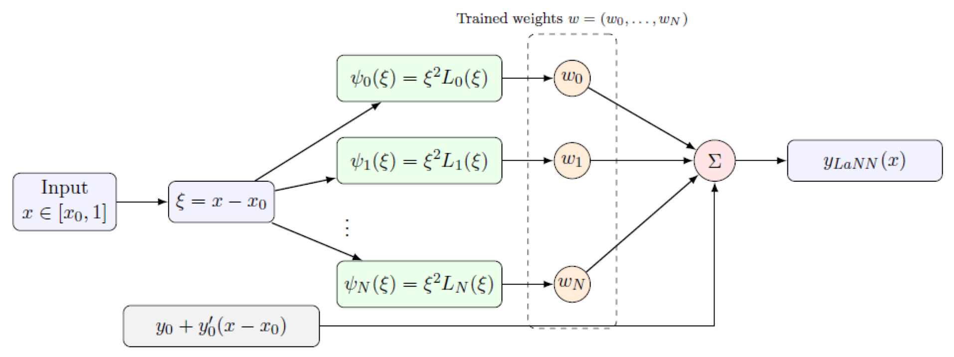
Figure 2.
Solution functions, loss, and error for Example 1 with a uniform distribution of collocation points.
Figure 2.
Solution functions, loss, and error for Example 1 with a uniform distribution of collocation points.
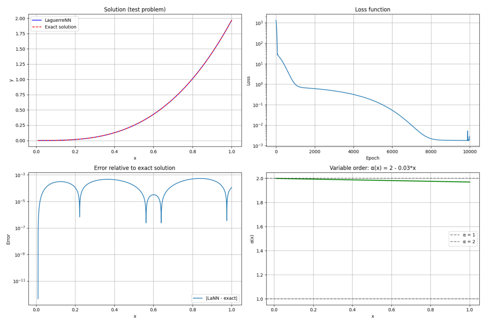
Figure 3.
Loss functions versus seeds.
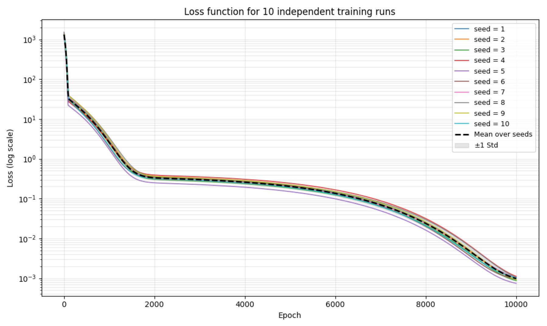
Figure 4.
Solution functions, loss, and error for Example 2 with a uniform distribution of collocation points and weight .
Figure 4.
Solution functions, loss, and error for Example 2 with a uniform distribution of collocation points and weight .
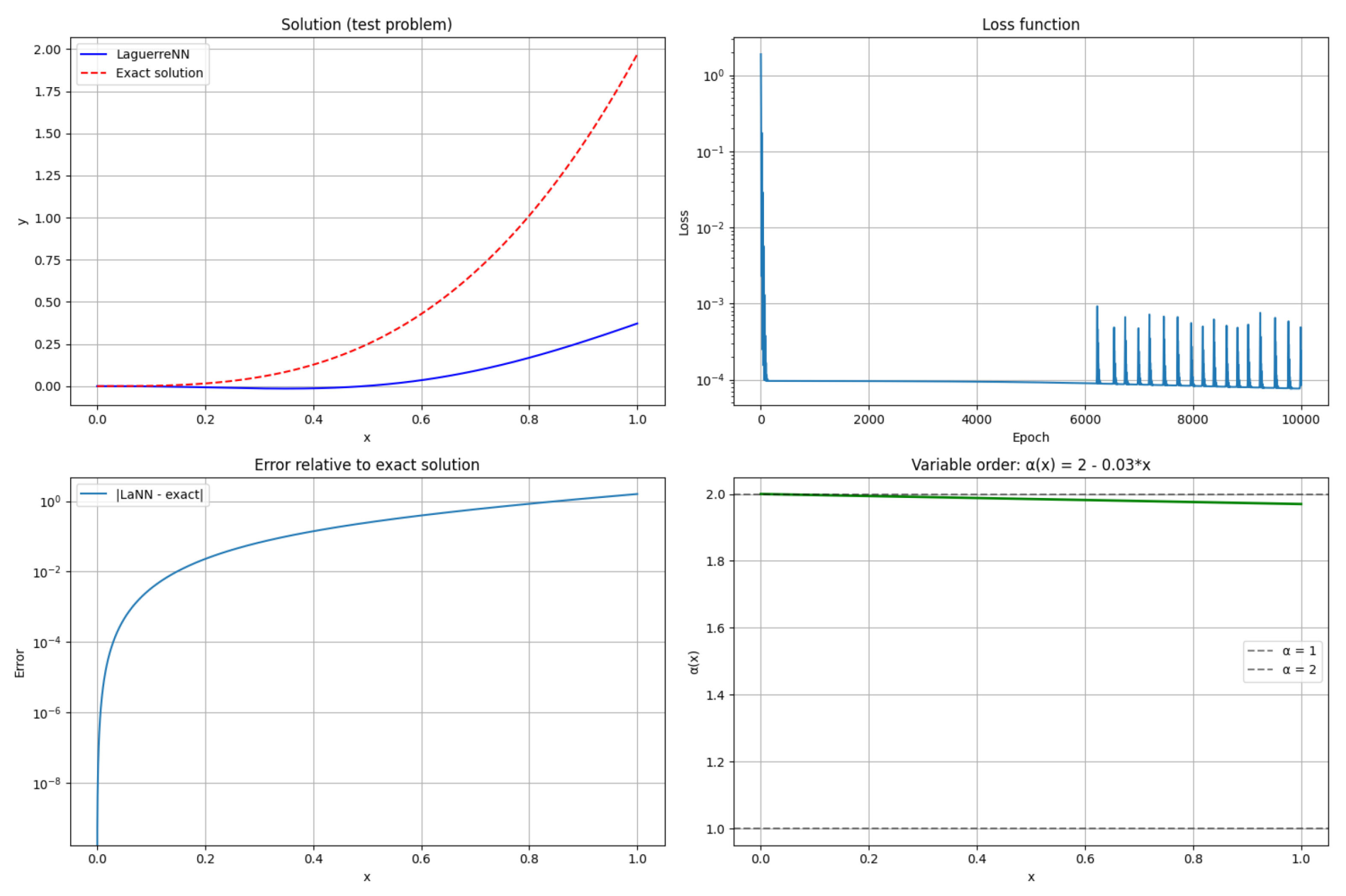
Figure 5.
Solution functions, loss, error, and fractional-derivative order for Example 4 with a uniform distribution of collocation points.
Figure 5.
Solution functions, loss, error, and fractional-derivative order for Example 4 with a uniform distribution of collocation points.
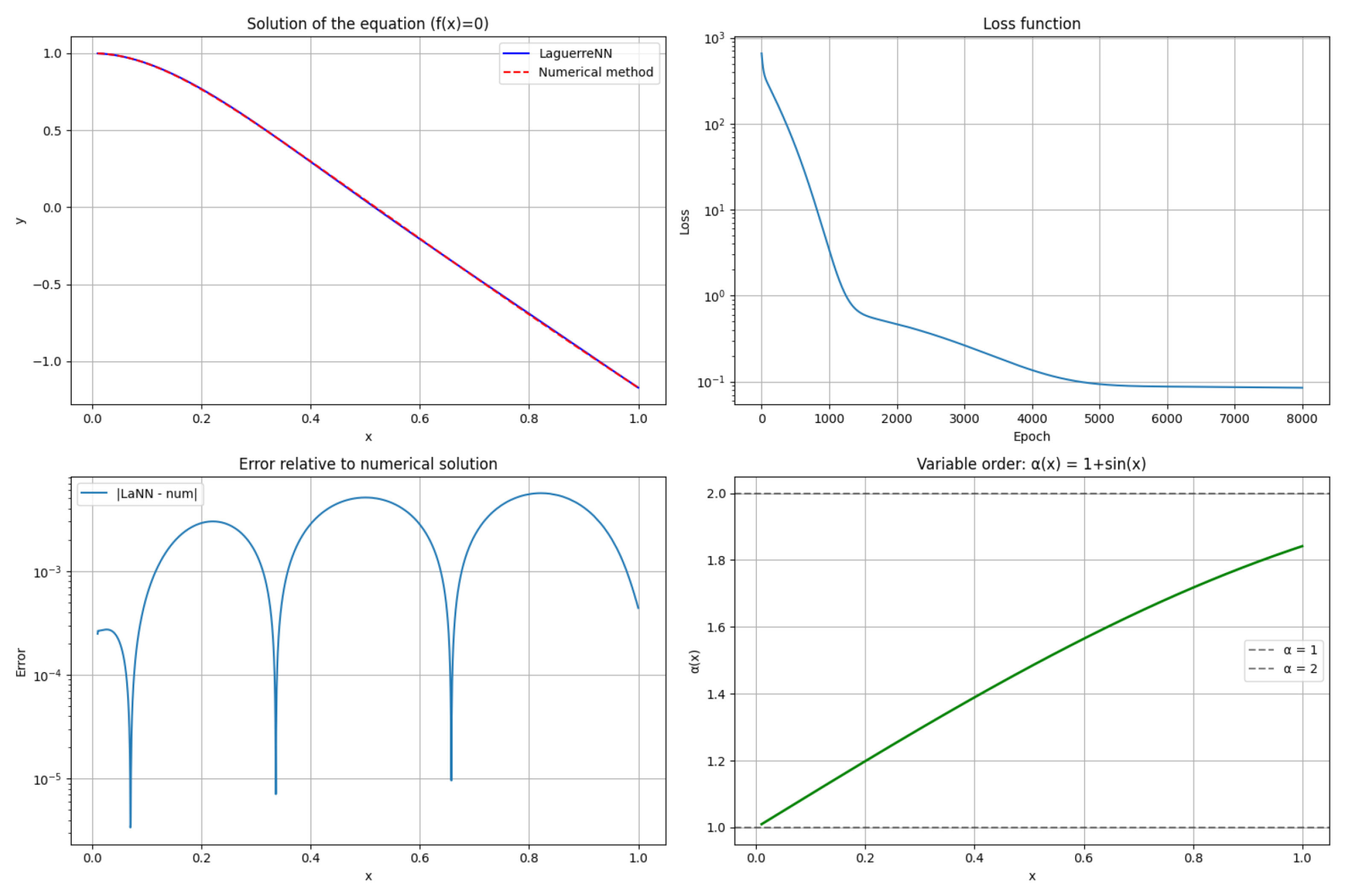

Table 1.
LaNN training hyperparameters.
| Hyperparameter | Value |
|---|---|
| Laguerre polynomial degree, N | 15 |
| Number of collocation points, M | 1000 |
| Number of epochs | 10,000 |
| Initial learning rate, | 0.005 |
| -regularization coefficient, | |
| Weight for the residual, | x |
Table 2.
Comparison of exact and neural-network solutions for Example 1.
| x | |||
|---|---|---|---|
| 0.0100 | |||
| 0.1200 | |||
| 0.2300 | |||
| 0.3400 | |||
| 0.4500 | |||
| 0.5600 | |||
| 0.6700 | |||
| 0.7800 | |||
| 0.8900 | |||
| 1.0000 |
Table 3.
Error metrics on 2000 test points uniformly distributed on the interval .
| Metric | Value |
|---|---|
| Maximum error (ME) | |
| Mean error (MAE) | |
| Root-mean-square error (RMSE) |
Table 4.
Reproducibility parameters of the computational experiment.
| Parameter | Value |
|---|---|
| Base random seed | 1 |
| Number of runs | 10 |
| Seeds | 1, 2, 3, 4, 5, 6, 7, 8, 9, 10 |
| Weight initialization | normal(0, 0.1) |
| Optimizer | Adam |
| learning rate | 0.005 |
| 1e-05 | |
| Scheduler | ReduceLROnPlateau |
| mode | min |
| patience | 500 |
| factor | 0.5 |
| min_lr | 1.0e-07 |
| threshold | 1.0e-04 |
| Early stopping | no |
| improvement type | relative |
| — | |
| patience | — |
| Device | cpu |
| torch.set_num_threads | 1 |
| PyTorch version | 2.7.1+cu118 |
| NumPy version | 2.1.3 |
| Python version | 3.13.1 |
Table 5.
Statistics over 10 independent training runs.
| Run | Seed | Best Loss | Epochs | Training time, s | ME | MAE | RMSE |
|---|---|---|---|---|---|---|---|
| 1 | 1 | 1.040e-03 | 10,000 | 13.08 | 6.136e-04 | 2.902e-04 | 3.411e-04 |
| 2 | 2 | 1.018e-03 | 10,000 | 13.12 | 6.205e-04 | 2.901e-04 | 3.419e-04 |
| 3 | 3 | 8.720e-04 | 10,000 | 13.11 | 5.662e-04 | 2.669e-04 | 3.140e-04 |
| 4 | 4 | 1.117e-03 | 10,000 | 13.32 | 6.679e-04 | 3.231e-04 | 3.773e-04 |
| 5 | 5 | 7.449e-04 | 10,000 | 14.04 | 4.994e-04 | 2.335e-04 | 2.747e-04 |
| 6 | 6 | 9.654e-04 | 10,000 | 13.71 | 5.698e-04 | 2.623e-04 | 3.088e-04 |
| 7 | 7 | 1.020e-03 | 10,000 | 13.70 | 6.068e-04 | 2.887e-04 | 3.388e-04 |
| 8 | 8 | 1.060e-03 | 10,000 | 13.67 | 6.517e-04 | 3.182e-04 | 3.703e-04 |
| 9 | 9 | 9.270e-04 | 10,000 | 13.69 | 5.836e-04 | 2.794e-04 | 3.274e-04 |
| 10 | 10 | 1.035e-03 | 10,000 | 13.77 | 6.167e-04 | 2.843e-04 | 3.352e-04 |
| Mean | — | 9.801e-04 | — | 1.352e+01 | 5.996e-04 | 2.837e-04 | 3.330e-04 |
| Std | — | 1.080e-04 | — | 3.366e-01 | 4.791e-05 | 2.610e-05 | 2.966e-05 |
Table 6.
Stability of metrics over 10 independent training runs.
| Metric | Mean | Std | Std/Mean, % |
|---|---|---|---|
| Best Loss | 9.801e-04 | 1.080e-04 | 11.02 |
| Training time, s | 13.5213 | 0.3366 | 2.49 |
| ME | 5.996e-04 | 4.791e-05 | 7.99 |
| MAE | 2.837e-04 | 2.610e-05 | 9.20 |
| RMSE | 3.330e-04 | 2.966e-05 | 8.91 |
Table 7.
Comparison of Laguerre and Legendre bases with identical settings (degree 15, 1000 collocation points, 10,000 epochs, lr=0.005, =1e-05, , seeds 1–5, 5 runs). All metrics are averaged over independent runs.
Table 7.
Comparison of Laguerre and Legendre bases with identical settings (degree 15, 1000 collocation points, 10,000 epochs, lr=0.005, =1e-05, , seeds 1–5, 5 runs). All metrics are averaged over independent runs.
| Basis | Best Loss | Std(Best Loss) | RMSE | ME | MAE | Train. time, s |
|---|---|---|---|---|---|---|
| Laguerre | 9.585e-04 | 1.488e-04 | 3.298e-04 | 5.935e-04 | 2.807e-04 | 13.382 |
| Legendre | 2.135e-03 | 4.289e-04 | 9.490e-04 | 1.808e-03 | 6.924e-04 | 13.561 |
Table 8.
Error analysis for Example 2 (uniform distribution).
| x | |||
|---|---|---|---|
| 1.0000e-10 | 2.000000e-30 | 2.000000e-30 | 0.000000e+00 |
| 0.1111 | 2.738912e-03 | -1.772174e-03 | 4.511085e-03 |
| 0.2222 | 2.187471e-02 | -8.485829e-03 | 3.036054e-02 |
| 0.3333 | 7.370371e-02 | -1.419560e-02 | 8.789931e-02 |
| 0.4444 | 1.744124e-01 | -8.611594e-03 | 1.830240e-01 |
| 0.5556 | 3.400778e-01 | 1.761026e-02 | 3.224675e-01 |
| 0.6667 | 5.866666e-01 | 7.007713e-02 | 5.165895e-01 |
| 0.7778 | 9.300366e-01 | 1.496592e-01 | 7.803774e-01 |
| 0.8889 | 1.385935e+00 | 2.527042e-01 | 1.133231e+00 |
| 1.0000 | 1.970000e+00 | 3.720084e-01 | 1.597992e+00 |
Table 9.
Error analysis for Example 2 (Chebyshev distribution).
| x | |||
|---|---|---|---|
| 1.0000e-10 | 2.000000e-30 | 2.000000e-30 | 0.000000e+00 |
| 0.1111 | 2.738912e-03 | 2.936242e-03 | 1.973307e-04 |
| 0.2222 | 2.187471e-02 | 2.180496e-02 | 6.975234e-05 |
| 0.3333 | 7.370371e-02 | 7.121572e-02 | 2.487995e-03 |
| 0.4444 | 1.744124e-01 | 1.680429e-01 | 6.369576e-03 |
| 0.5556 | 3.400778e-01 | 3.317674e-01 | 8.310407e-03 |
| 0.6667 | 5.866666e-01 | 5.823949e-01 | 4.271686e-03 |
| 0.7778 | 9.300366e-01 | 9.373112e-01 | 7.274628e-03 |
| 0.8889 | 1.385935e+00 | 1.408024e+00 | 2.208889e-02 |
| 1.0000 | 1.970000e+00 | 1.997429e+00 | 2.742910e-02 |
Table 10.
LaNN training times depending on various weights and collocation-point distributions.
| Collocation points | Uniform distribution | Chebyshev distribution | ||||
|---|---|---|---|---|---|---|
| , s | 12.94 | 13.06 | 13.22 | 12.92 | 13.05 | 14.24 |
| , s | 381.42 | 398.85 | 394.46 | 395.62 | 389.74 | 394.65 |
Table 11.
Error analysis for Example 3.
| x | |||||||
|---|---|---|---|---|---|---|---|
| 0.01 | |||||||
| 0.12 | |||||||
| 0.23 | |||||||
| 0.34 | |||||||
| 0.45 | |||||||
| 0.56 | |||||||
| 0.67 | |||||||
| 0.78 | |||||||
| 0.89 | |||||||
| 1.00 |
Table 12.
Error analysis for Example 4.
| x | Error | ||
|---|---|---|---|
| 0.010 | |||
| 0.120 | |||
| 0.230 | |||
| 0.340 | |||
| 0.450 | |||
| 0.560 | |||
| 0.670 | |||
| 0.780 | |||
| 0.890 | |||
| 1.000 |
Table 13.
Inference time measurements.
| Run number | Time, s |
|---|---|
| 1 | |
| 2 | |
| 3 | |
| 4 | |
| 5 | |
| 6 | |
| 7 | |
| 8 | |
| 9 | |
| 10 |
Table 14.
Measurement of neural-network inference time (10 runs).
| Parameter | Value |
|---|---|
| Test sample size | 2000 |
| Mean time of one inference, s | |
| Standard deviation, s | |
| Minimum / maximum, s | / |
| Mean time per point, s |
Disclaimer/Publisher’s Note: The statements, opinions and data contained in all publications are solely those of the individual author(s) and contributor(s) and not of MDPI and/or the editor(s). MDPI and/or the editor(s) disclaim responsibility for any injury to people or property resulting from any ideas, methods, instructions or products referred to in the content. |
© 2026 by the authors. Licensee MDPI, Basel, Switzerland. This article is an open access article distributed under the terms and conditions of the Creative Commons Attribution (CC BY) license (http://creativecommons.org/licenses/by/4.0/).
Copyright: This open access article is published under a Creative Commons CC BY 4.0 license, which permit the free download, distribution, and reuse, provided that the author and preprint are cited in any reuse.