

Submitted:
24 September 2026
Posted:
24 September 2026
You are already at the latest version
Abstract
Hyperspectral Image Classification is an importanttopic in remote sensing with numerous applications in precision agriculture, environmental monitoring, defence, and more. It helps classify material composition by mapping spectral signatures from each pixel. Despite its potential, it faces persistent challenges due to the scarcity of labelled data and high dimensionality. This makes it difficult to achieve robust performance that can generalize well. To address this problem, we propose SRSSF (Stability-Reliability Spectral-Spatial Fusion), a hybrid mixture-of-experts framework for hyperspectral image (HSI) classification. It fuses a compact, stability-selected spectral representation with full-spectrum spatial and joint spectral-spatial descriptors (extended morphological, attribute-like, and Gabor texture profiles), combined through validation-derived reliability weights rather than fixed or heuristic fusion rules. SRSSF is evaluated under a strict, footprint-level spatially disjoint protocol in which entire patch receptive fields are guaranteed non-overlapping across training, validation, and test partitions, not mere center pixels. It has an automated, geometry-only (label- and accuracy-independent) seed-acceptance procedure and requires a minimum dataset-specific test-set size for training. The framework is benchmarked against fourteen classical and CNN spectral/spatial baselines and a dedicated ablation suite, across four benchmark datasets (Indian Pines, Pavia University, Salinas, and the Kennedy Space Center (KSC)). Our framework achieves the best OA, AA, and κ on every dataset, with OA scores of 56.43,91.94,90.50, and 75.96 at Indian-Pines, Pavia University, Salinas, and KSC, respectively.
Keywords:
hyperspectral image classification
; spatial spectral fusion
; band selection
; machine learning
; remote sensing
1. Introduction
The classification of hyperspectral images [1] remains a challenge in remote sensing. It helps in disaster tracking and management, urban planning, mining, defence and surveillance, and more [2]. Each pixel is a vector of hundreds of values from emitted, transmitted, absorbed, or reflected electromagnetic waves off different surfaces or objects [3], which vary by material type and span different ranges: visible, near-infrared, shortwave-infrared, and thermal-infrared. It contains both spatial and spectral information that helps to classify objects and other information properly, impossible with an RGB image due to similar visual identity but different material composition. This large spatial variability of spectral signatures, paucity of data, atmospheric and sensor noise, redundant data, and high dimensionality make it difficult to extract and process meaningful information [4]. Different solutions exist that can be grouped into six different categories based on their functionality: band selection, dimensionality reduction, spectral-spatial feature extraction, pixel-wise classification, hybrid ensemble methods, and deep learning approaches. Pixel-wise classifiers like support vector machine (SVM) [5], K-nearest neighbor [6], etc., are the earliest naive classifiers used for a wide range of supervised classification tasks. However, they suffer from the curse of high dimensionality and computational cost. So, dimensionality reduction algorithms, e.g., principal component analysis (PCA) [7], linear discriminant analysis (LDA) [8], or independent component analysis (ICA) [9], and band selection algorithms like Mutual Information (MI) [10], Sequential Forward Floating Selection (SFFS) [5], L1-regularized embedded (LASSO) [11], and correlation pruning [12] are used along with pixel-wise classifiers to improve results. However, these results are unsatisfactory, as it completely ignores the spatial information - shape, structure, etc.- has high spectral variability and redundancy. Therefore, spectral-spatial classifiers such as extended morphological profile (EMP) and Support Vector Machine (SVM) [13], Gabor and SVM [14], extended attribute profile (EAP) and SVM [15], etc., have been developed to improve classification accuracy. However, these methods require large amounts of data and significant computational resources to achieve robust performance and scalability. More recently, hybrid approaches have emerged, which can be broadly divided into classical Machine learning (ML) ensembles, e.g., SVM + Random Forest (RF) [16], and machine learning + deep learning hybrids, e.g., EMP features fused with convolution neural network (CNN), EMP + CNN [17]. In parallel, purely deep learning pipelines such as 3D CNNs [18] and transformers [19] have been explored. Deep learning-based approaches are data-hungry with high computational cost; extensive GPU requirements, less interpretability, and reproducibility issues make them a poor choice. Our SRSSF framework belongs to the class of classical machine learning hybrid ensembles, distinct from ML+DL hybrids and pure deep learning pipelines. By combining stability-selected spectral experts with spatial and joint experts under reliability weighting, SRSSF achieves interpretable and reproducible gains without relying on deep neural architectures. Our main contributions:
- We propose SRSSF, a reliability-weighted mixture-of-experts combining a stability-selected spectral expert with full-spectrum spatial and joint experts, plus a compact-input ablation (SRSSF-SelectedInput) to isolate band-restriction effects.
- We design a shared validation-only band selection that fixes a single spectral budget per dataset/seed, applied consistently across models and ablations, avoiding test-set influence.
- We introduce a strict footprint-disjoint protocol for patch-based HSI classification, enforcing zero overlap between train/val/test receptive fields and using automated geometry-based seed acceptance.
- We pair benchmarks with interpretability analysis, including SHAP feature attribution, band-stability visualization, and expert-reliability reporting to reveal which bands and experts drive decisions.
2. Related Work
Pixel-wise classifier. Pixel-wise classifiers assign labels independently per pixel, ignoring spatial context. They are computationally light but often inaccurate. SVM [5] is widely used due to low data requirements and resistance to overfitting. It maps overlapping data into higher dimensions for separability and scales from binary to multi-class. However, in high-dimensional spectral spaces, sparsity and redundancy cause overfitting, poor weighting of bands, and heavy parameter search costs. KNN [6] classifies by local neighborhoods without distributional assumptions, performing well with small, irregular datasets, but suffers in high dimensions where distances lose meaning and generalization is weak. RF [20] ensembles decision trees over random feature subsets, reducing noise sensitivity, yet struggles in heterogeneous regions with overlapping spectra.
Dimensionality reduction and band selection. Pixel-wise classifiers suffer from high-dimensionality and redundant bands, so dimensionality reduction (PCA, LDA, ICA, KPCA [7,8,9,21]) and band selection (MI, correlation pruning [12], SFFS, LASSO) are widely used. PCA is unsupervised, reduces redundancy/noise, but is weak in discrimination. LDA is supervised, maximizes class separability, yet struggles with non-linear boundaries. ICA extracts independent components for spectral unmixing but is noise-sensitive and computationally heavy. KPCA extends PCA to non-linear manifolds but depends critically on kernel choice and is expensive. MI [10] captures non-linear dependencies for feature selection but requires reliable probability estimates. SFFS [5] dynamically adds/removes features, flexible but prone to overfitting and costly. LASSO [11] embeds selection during training, yielding sparse solutions well-suited to high-dimensional HSI, though sensitive to regularization and may discard correlated useful bands.
Spectral-spatial classifier. Spectral classifiers (e.g., SVM with PCA [7]) reduce dimensionality and denoise but ignore spatial context, limiting accuracy. EMP+SVM [13] adds morphological filters for spatial coherence, simple and interpretable but sensitive to structuring elements, heavy for large images, and prone to overfitting. EAP+SVM [15] generalizes EMP with attribute filters (area, deviation, moment), offering more flexibility and typically higher accuracy. Gabor+SVM [14] incorporates texture and orientation cues, effective for urban/man-made structures, but requires careful parameter tuning and is less suited to natural scenes with irregular textures.
Hybrid approaches. Spectral–spatial methods improved accuracy but lacked robustness and scalability. Hybrid approaches emerged to stabilize performance (ensembles), reduce redundancy (band selection), balance dimensionality (PCA/LDA), and exploit new paradigms (ML, DL, self-supervised, RL). Spectral–spatial gave context; hybrids added integration and resilience. Traditional ML hybrids (e.g., SVM+RF [16]) are more resilient to overfitting, while ML+DL hybrids (e.g., EMP+CNN [17]) learn local features and their interactions better. These improve accuracy under limited labels, scale well, but risk redundancy, complex pipelines, and tuning challenges.
Deep Learning. Deep learning supersedes hybrids in accuracy under abundance of labelled data, but hybrids remain relevant for interpretability and robustness under limited data. It is end-to-end learning; it requires no handcrafted features and achieves state-of-the-art accuracy on benchmark datasets. CNN [18] and transformer-based [19] architectures are typically used.
We acknowledge both hybrid categories and higher variants of deep learning pipelines, but our work focuses on classical ML ensembles. We do not compare against ML+DL hybrids or higher variants of deep learning baselines (2D/3D CNNs), as our emphasis is on reproducible, interpretable traditional methods. Higher variants of DL (2D/3D CNNs) depend on spatial overlap, making them incompatible with our footprint-disjoint evaluation.
3. Methodology
This section describes the spatially disjoint evaluation protocol used to prevent patch-level leakage, the classical and deep-learning baselines, the proposed Stability-Reliability Spectral-Spatial Fusion (SRSSF) architecture (Figure 1), the shared band-count selection procedure, the full algorithmic pipeline, and the interpretability methodology used throughout this study.
3.1. Spatially Disjoint, Leakage-Free Split Protocol
A major concern in HSI is that neighboring pixels are highly correlated and share similar spectra. When patch-based descriptors are used, these pixels overlap, leading to biased accuracy since the model has effectively seen similar data. To prevent such leakage, we adopt a strict footprint-disjoint sampling strategy at the level of patch footprints, rather than relying only on center pixels.
3.1.1. Footprint Locking
For a candidate center pixel and patch size p, definition of its footprint as the square neighborhood: Eq.(1)
Boolean masks, and , of size track pixels already locked by train or validation footprint, respectively. A center is footprint-free with respect to a mask M if contains no True entries.
Training and validation centers must be footprint-free relative to and , ensuring no overlap between patches within or across these sets. This stricter no-overlap rule minimizes spatial redundancy in development data used for stability scoring, expert models, and fusion weights. Only test patches may overlap (Section 3.1.3), since they are excluded from fitting, band selection, and fusion-weight estimation; overlap confined to the test set does not constitute leakage.
3.1.2. Per-Class Training and Validation Selection
For each class and random seed S, class- and seed-specific random states are used to shuffle the coordinates of all labelled pixels of class k. Fixed fractions of and , per dataset, are used to compute a target number of training centers and validation centers (Table 1):
where is the set of labelled pixels of class k; validation centers are reserved first. Training centers are fetched from the remaining candidates, under the strict constraint that each of their footprints is simultaneously free of and . Once accepted, a center’s footprint is locked into its corresponding mask. This guarantees that no training footprint intersects any validation footprint.
3.1.3. Strict Test Selection
A labelled pixel is assigned to the test set only if its entire footprint is free of both and :
It is strictly stronger than selecting center pixels after excluding train and val center pixels, which would have allowed a test patch to share up to pixels with a training or validation patch. Test patches are allowed to overlap one another, since test samples never participate in parameter fitting, band selection, or fusion-weight estimation; overlap confined to the test partition does not constitute leakage.
3.1.4. Adaptive Density Relaxation
In datasets with small or spatially fragmented classes (notably KSC [22]), strict exclusion of training and validation data may leave little or no test data. To address this, target counts for training and validation are scaled by a factor , halved iteratively (up to six attempts) until a non-empty test region is obtained. If no valid outcome is found, a relaxed fallback (center-pixel exclusion only) is applied, and the split is explicitly flagged as non-strict. Such relaxed splits are excluded from the accepted-seed pool described in Section 3.2.
3.1.5. Leakage Verification
For every candidate split, three binary footprint masks are rasterized from the accepted train, validation, and test centers, and pairwise pixel-wise intersections are computed: Eq.(4).
A split is considered leakage-free if and only if . This check is performed independently of, and after, the split construction, so that any residual overlap is measured directly on the realized footprints rather than assumed from the sampling procedure.
3.2. Seed Filtering for Statistically Reliable Evaluation
3.2.1. Seed Selection
Because footprint locking is greedy and order-dependent, the number of centers per partition varies across random seeds. To ensure leakage-free and statistically meaningful results, we select exactly acceptable seeds per dataset from candidates . A seed is accepted only if:
- 1.
- the split is strict (non-empty test set without density relaxation);
- 2.
- all three pairwise footprint overlaps are zero;
- 3.
- the number of test centers meets the dataset-specific minimum (Table 2).
Acceptance depends solely on split geometry and ground-truth labels; no classifiers are fit, and no test predictions are used, preventing bias. The R accepted seeds are reused consistently across all experiments (main comparison, per-class analysis, few-shot, ablation, and efficiency benchmarking).
3.3. Data, Feature, and Band-Count Sharing/Caching Protocol
To ensure fair comparisons, we separate cached data (for reuse only) from shared splits/features (for methodological fairness). Normalized cubes, labels, and global EMP/EAP/Gabor [13,14,15] maps are cached once per dataset. Within each evaluation condition (dataset, seed, experiment type), identical splits, labels, raw spectra, and shared band-count are passed to all methods. Baseline transforms (PCA, ICA, SpaBS, MVPCA [5,7,9,23,24]) and SRSSF band indices are recomputed independently, while few-shot experiments construct distinct splits per shot count.
3.4. Spatial and Spectral Feature Extraction
Three complementary spatial feature stacks are computed for each accepted split, once per dataset from the grayscale image and cached for reuse across all train, validation, and test centers.
Extended Morphological Profile (EMP). Disk-shaped structure elements with radii are applied with grayscale morphological opening and closing, yielding a six-channel morphological stack; mean filters with window sizes are applied as a fallback when no morphology library is available.
Extended Attribute Profile (EAP) surrogate. Grayscale images are binarized with four intensity thresholds , and a mean filter smooths each binary mask and its complement, producing an eight-channel attribute-like stack.
Gabor filter bank. Three spatial frequencies and four orientations are used to construct a bank of Gabor kernels, via FFT-based convolution, yielding a twelve-channel texture stack.
Spectral vectors are extracted directly as for a coordinate set , and the corresponding rows of the cached EMP, EAP, and Gabor stacks are gathered at the same coordinates.
3.5. Classical and Deep-Learning Baselines
We evaluate 15 configurations: 13 classical baselines (7 spectral-only, 5 spatial-spectral, and 1 deep-learning) together with the two proposed SRSSF variants. All models are fit and evaluated identically on each accepted split, all fit identically on each accepted split.
Spectral-only: Raw+SVM [5] uses standardized spectra with an RBF-SVM (, ). PCA+SVM [7] and FastPCA+RF [25,26] project onto 30 principal components (standard vs. randomized SVD), followed by SVM or RF (200 trees, depth 25). ICA+SVM [9] applies FastICA with whitening, falling back to PCA if unstable. KPCA+SVM [21] uses Nyström RBF with 300 landmarks plus PCA before SVM. SpaBS+SVM [5,23] selects 30 bands by variance, while MVPCA+SVM [5,24] ranks bands by loadings of 10 FastPCA components.
Spatial-spectral: EMP+SVM [13], EAP+SVM [15], and Gabor+SVM [14] concatenate spectra with spatial features. EMP+RF [13,26] applies RF (200 trees, depth 25) to EMP-augmented inputs. SVM+RF [16] is a soft-voting ensemble of RBF-SVM and RF on raw spectra.
Deep learning: Spectral1DCNN is a lightweight 1D CNN [27] trained on standardized spectra (B bands as a length-B sequence). It has three convolutional blocks (kernels ; channels ; BN, ReLU, pooling) and a two-layer head with dropout (). Training uses Adam ( lr, wd) for 60 epochs, batch size 64. If PyTorch is unavailable, Raw+SVM is substituted and logged.
3.6. Proposed SRSSF Architecture
The proposed Stability-Reliability Spectral-Spatial Fusion (SRSSF) model is a mixture-of-experts architecture that combines full-spectrum spatial and joint representations with a compact, stability-selected spectral representation, fused via reliability weights derived from evaluation on the validation set.
3.6.1. Stability-Selected Band Subset
Given training spectra and labels , band relevance is estimated via class-stratified bootstrap resamples (sampling fraction per class). For each bootstrap t, a one-way ANOVA F-score is computed per band b using f_classif.
The mean and standard deviation of across bootstraps define a stability-adjusted score with stability penalty . (Eq.(6))
with stability penalty . Bands are ranked in descending order of and greedily accepted into a subset of size k subject to a redundancy constraint: a candidate band is admitted only if
where is the Pearson correlation coefficient; If Eq.(7) is satisfied by fewer than k bands, the redundancy filter is not used in ranking to guarantee exactly k selected bands.
3.6.2. Expert Feature Blocks
Let denote the spectrum restricted to the stability-selected band subset . The spectral–spatial input is defined as for SRSSF(Ours) and for SRSSF-SelectedInput. The seven expert feature blocks are
Here, ∥ denotes column-wise concatenation and is randomized-SVD PCA with at most 30 components, fit using the training partition and applied unchanged at inference. Thus, SRSSF(Ours) uses selected bands only for the spectral expert while retaining the full spectrum in all spatial and joint experts. In SRSSF-SelectedInput, is replaced by , so every expert operates on the same compact selected-band representation.
3.6.3. Expert Classifiers and Reliability-Weighted Fusion
Each expert block trains an independent classifier: an RBF-SVM () for spectral, emp, eap, gabor, and joint; a random forest (200 trees, depth 25) for rf and fastpca_rf. Each classifier produces class-probability estimates on the held-out validation partition, and per-expert validation accuracy is computed. Reliability weights are obtained via a softmax over validation accuracy with temperature :
At inference, per-expert class-probability vectors are combined as
and the predicted label is . After the validation-based fusion weights are fixed, all expert classifiers (and, where applicable, the PCA projection) are refit on the union of validation and training data, restricted during initial fit. So the final deployed model benefits from the additional validation samples without altering the reliability weights, computed from the held-out validation predictions.
3.7. Shared Band-Count Selection
Once k stability bands are selected per seed and dataset from the train and validation partition only, we use it across all methods and ablation configurations for both variants of SRSSF. For each candidate , the hybrid architecture (SRSSF(Ours), select_input_mode=False) is fit on the train partition and evaluated on the validation partition, yielding validation OA. The smallest k within a tie tolerance of percentage points of the best observed validation OA is selected:
Compact spectral representations are favored over larger ones if it is meaningful. This guarantees that the test partition is never touched, except at final testing. All band-count sweeps and the resulting per dataset/seed are logged for reproducibility.
3.8. Ablation Configurations
To isolate the contribution of stability-based band selection and reliability-weighted fusion, six configurations are compared under identical splits and shared : (i) RawSVM, an RBF-SVM on the full raw spectrum; (ii) SRSSF_SpectralOnly_WithSelection, an RBF-SVM trained only on the stability-selected bands ; (iii) SRSSF_FusionNoBandSelection, the full hybrid fusion architecture with the spectral expert forced to use all B bands instead of ; (iv) SRSSF_UniformFusion, the hybrid fusion architecture with reliability weights replaced by a uniform average ; (v) SRSSF(Ours); and (vi) SRSSF-SelectedInput.
3.9. Interpretability and Explainability
Beyond aggregate accuracy metrics, we report three complementary interpretability analyses, each computed per dataset, seed, and experiment type, and subsequently aggregated across the R accepted seeds.
3.9.1. Shapley-Value Feature Attribution (SHAP)
For every classical baseline and for the 1D-CNN, feature-level attributions are computed using Shapley additive explanations (SHAP). For a trained probability model , the SHAP value of feature j for instance is defined as the Shapley value of j in the cooperative game whose value function is the model’s expected output over feature subsets:
where is the full feature index set and is the model output when only the features in S are set to their values from and all others are marginalized using a background sample. In practice, is estimated with a model-agnostic Explainer using a background set of 20 training instances and an explanation set of up to 50 test instances per (dataset, seed, experiment, method) combination. Per-feature importance is summarized as the mean absolute SHAP value over the explanation set,
and the top-20 features ranked by are reported, along with aggregate summaries averaged over all R accepted seeds and, separately, over all evaluated methods. SHAP attribution is not computed for the 1D-CNN’s internal convolutional activations, since perturbation-based explainers are not directly applicable to raw sequence inputs; this limitation is explicitly noted in the explainability artifacts.
3.9.2. Band-Stability Diagnostics
For each SRSSF instance, the per-band mean , standard deviation , stability score (Eq. (6)), and binary selection indicator are saved and visualized as stability curves with selected bands highlighted. Aggregation across R seeds averages , and selection frequency , yielding a seed-robust view of consistently discriminative spectral regions.
3.9.3. Expert Reliability Diagnostics
For each SRSSF instance, the global expert reliability weight (Eq. (9)) and corresponding per-class weight (identical across classes under the current scheme) are saved and visualized as bar charts over the seven experts (Eq. (8)). Aggregating across R seeds highlights which experts (spectral, EMP, EAP, Gabor, joint, RF, FastPCA-RF) are consistently most reliable, complementing the model-agnostic SHAP attributions.
4. Experiments
4.1. Datasets
This study employs four benchmark hyperspectral datasets: Indian Pines, Pavia University, Salinas, and Kennedy Space Center(KSC) - [22]. Indian Pines: 220 bands (200 retained), 16 crop/vegetation classes, 145×145 pixels. Pavia University: 115 bands (103 retained, 0.43–0.86µm), 9 urban classes, 610×340 pixels. Salinas: 224 bands (204 retained), 16 agricultural classes (broccoli, celery, grapes, lettuce, vineyards, fallow, stubble, soils), 512×217 pixels. KSC: 224 bands (176 retained), 13 vegetation/water classes, 512×614 pixels.
Each dataset contains spatial pixels and B spectral bands, along with ground-truth label map . C is the number of land-cover classes, where class 0 denotes unlabelled background. Each cube is min-max normalized to using the global minimum and maximum of the full cube, before any experiment:
, prevents division by zero. Details of the fixed square patch size p used for spatial feature extraction and footprint locking for each dataset d are shown in Table 3.
4.2. Evaluation Metrics
Performance is evaluated on the held-out test centers using overall accuracy (OA), average accuracy (AA), Cohen’s kappa coefficient () Eq.(16), and per-class accuracy, precision, recall, and F1-score. Let denote the test confusion matrix, where is the number of pixels of true class i classified as class j. OA and AA are defined as
Cohen’s Eq.(16) is computed from the same confusion matrix to account for chance agreement. Precision, recall, and F1-score are reported separately for each class in the per-class analysis. F1 mean score is calculated as:
Structural Breakdown, : The diagonal elements (correctly classified land-cover pixels for class : The row sum for class i, representing total ground truth pixels (User’s / Producer’s base reference). : The column sum for class i, representing all pixels assigned to that class by the model.
All results are reported as mean ± standard deviation over the ten accepted seeds; the realized number of successful runs is also reported for each dataset–method pair.
4.3. Implementation Details
All experiments are completed on a 64-core CPU with 432 GB RAM. The global NumPy seed is fixed to 42, while each stochastic split, bootstrap resampling, classifier initialization, and CNN run is controlled by its accepted seed for exact reproducibility. Threading-sensitive libraries (OpenMP, OpenBLAS, MKL, NumExpr) are pinned to a single thread to ensure deterministic behavior. Explainability artifacts, per-band stability scores and indicators, per-expert reliability weights, and SHAP-based feature-importance summaries (Section 3.9), are saved per dataset, experiment type, and seed, then aggregated across R accepted seeds. Split-quality diagnostics, strictness flags, footprint-overlap counts (Eq. (4)), and realized train/validation/test center counts are persisted for every seed to fully audit the leakage-free protocol (Section 3.1) and caching/sharing behavior (Section 3.3).
5. Results
The proposed SRSSF framework is evaluated on four benchmark hyperspectral datasets under strict footprint-disjoint splits, with comparisons to classical ML and 1D CNN baselines. Results are reported as mean ± std over accepted, leakage-free seeds per dataset (Section 3.2). Section(Section 5.1) gives quantitative table outputs; Section(Section 5.2) summarizes the qualitative visual results.
5.1. Quantitative Results
5.1.1. Main Comparison
Table 4 reports OA, AA, and for all fifteen methods on all four datasets. SRSSF(Ours) attains the best OA, AA and on every dataset (OA: / / / on Indian Pines/Pavia University/Salinas/KSC respectively [22]), with the largest AA margin over the best baseline on KSC ( vs. , EMP+SVM [13]) and Indian Pines ( vs. , Gabor+SVM [14]), indicating gains concentrated on under-represented classes. KPCA+SVM [21] collapses on KSC ( OA), reflecting Nyström instability on sparse label geometry. 1D-CNN [27] is weakest everywhere (e.g., OA on KSC), consistent with limited data under strict disjoint splits. PCA+SVM [7]/ICA+SVM [9] are near-identical (ICA falls back to PCA on convergence failure). SRSSF-SelectedInput trails SRSSF(Ours) on every dataset (e.g., OA on Indian Pines) yet still beats all thirteen non-SRSSF baselines on Pavia University and KSC in OA.
5.1.2. Few-Shot Sensitivity
Table(Table 5) reports OA at 5–25 samples/class. SRSSF(Ours) leads at nearly every budget on all datasets (SRSSF-SelectedInput is not considered for comparison against SRSSF(Ours)), with the largest relative margin at the lowest budget on Pavia University ( vs. for FastPCA+RF [25,26], at 5 shots/class), confirming that stability-selected spectral features and reliability fusion are most valuable when labels are scarce. Ensemble/variance baselines (SVM+RF [16], SpaBS+SVM [5,23]) close or reverse the gap only at the largest budget on Indian Pines (/ vs. at 25 shots/class) and KSC ( vs. ), while KPCA+SVM [21] and 1D-CNN [27] are unstable at low shots on KSC (e.g., KPCA+SVM: OA at 5 shots/class). AA and Kappa showed consistent trends with OA across all datasets, so we report OA only in few-shot tables.
5.1.3. Computational Efficiency
Efficiency analysis in Table 6 shows that while classical methods are fastest and most memory-efficient, they sacrifice accuracy. Deep learning and the proposed SRSSF framework incur higher training cost, but inference remains sub-second. The Selected-Input variant further reduces memory and inference time, making SRSSF practical for real-world hyperspectral applications.
5.2. Qualitative Results
Split maps The split maps in Figure 2 confirm leakage-free partitions across all four datasets: green train centers, blue validation centers, and red test centers, with gray marking footprint-locked exclusion zones. Among them, KSC exhibits the sparsest and most fragmented labelled regions, reflecting the reduced training and validation counts imposed by the strict footprint-disjoint protocol. (Section(Section 3.1)).
Classification maps (Figure 3) The classification panel presents the false-color composite, grayscale image, ground truth, and per-method prediction maps for Indian Pines (seed=0). While qualitative maps under strict footprint-disjoint splitting appear fragmented, they illustrate the relative coherence of SRSSF compared to classical baselines. The figure is included for transparency, showing that visual artifacts stem from label scarcity and spatial disjointness rather than methodological flaws. It is in Table 4.
Per-class F1 heatmap (Figure 4) The heatmap consolidates per-class F1 across all fifteen methods and four datasets. SRSSF attains the highest mean per-class F1 overall (, vs. for the best classical baseline, EMP+SVM) and ranks among the top three methods on of classes, though it is not uniformly best at the individual-class level — several spatial baselines remain competitive on specific classes. On Indian Pines, rare classes with only a handful of labelled pixels (Alfalfa, Grass-pasture-mowed, Oats) yield near-zero F1 across all methods, confirming a label-scarcity ceiling rather than a method-specific weakness. On KSC, Oak/Broadleaf and Hardwood remain the hardest classes for SRSSF (F1 ), pointing to spectral confusion among visually similar wetland vegetation types as the dominant remaining error source.
Band-stability curves (Figure 5) Selected bands concentrate within compact, dataset-specific spectral regions rather than spreading uniformly, with the stable sub-bands’ location and spread varying across datasets. This indicates that the stability criterion adapts to each scene’s discriminative spectral structure rather than applying a fixed selection pattern.
Expert-reliability weights (Figure 6) Across datasets, SRSSF emphasizes different experts depending on scene characteristics. In KSC, FastPCA-RF dominates, indicating that spectral dimensionality reduction captures most discriminative variance. In Indian Pines, the RF expert leads, reflecting the importance of spatial–spectral fusion in heterogeneous agricultural fields, with FastPCA-RF secondary. In Pavia University, EMP receives the highest weight, consistent with the relevance of morphological profiles for urban structures, with Joint features close behind. In Salinas, FastPCA_RF receives the largest weight, while other experts contribute diffusely, indicating that spectral compression is most reliable but spatial cues provide complementary support. These results confirm that SRSSF adaptively prioritizes the most informative experts according to dataset properties.
SHAP attributions (Figure 7) The SHAP heatmap shows that classical spectral baselines and SRSSF’s spectral expert emphasize overlapping but non-identical band regions, confirming that stability selection retains genuinely discriminative spectral cues rather than an arbitrary subset of baseline features.
Taken together, section(Section 5.2) forms a coherent narrative: SRSSF gains accuracy by enforcing leakage-free partitions, emphasizing compact stable spectral regions, and adaptively weighting spatial–spectral experts. Residual errors stem from label scarcity and spectral confusion, highlighting both the strengths and remaining challenges of the framework.
6. Ablation Study
Table(Table 7) isolates band selection and reliability fusion using six configurations, on identical splits and shared .
Three findings emerge. Spectral-Only+Selection, discarding all spatial context, is the weakest SRSSF-family configuration everywhere (e.g., OA vs. SRSSF(Ours) on Indian Pines), showing spatial context, not spectral compaction, drives most of SRSSF’s accuracy. Fusion-No-Band-Selection performs statistically comparably to, and marginally above, SRSSF(Ours) on all four datasets. This indicates that band selection’s main benefit is dimensionality reduction of the spectral expert at negligible accuracy cost, more consequential for the compact SRSSF-SelectedInput variant. Replacing validation-derived reliability weights with uniform averaging costs – OA points on every dataset, a modest but consistent margin confirming reliability weighting reliably improves over naive averaging.
7. Discussion
Implications. Implications. SRSSF yields the best OA/AA/, with the largest gains under label scarcity and spectral confusion, driven primarily by reliability-weighted fusion. Band selection contributes negligible additional accuracy on its own (SRSSF_FusionNoBandSelection matches or marginally exceeds SRSSF(Ours) in the ablation). Still, it delivers the framework’s efficiency and compactness gains at essentially no accuracy cost.
Comparison. Classical spatial descriptors (EMP [13]/EAP [15]/Gabor [14]) improve over raw spectra but less than SRSSF’s learned fusion, underscoring that expert combination matters. Unlike prior work, we enforce footprint-disjoint splits and report variance across seeds for stricter evaluation.
Limitations. Gains incur up to fit-time and memory (excluding 1D-CNN). Extreme scarcity (<10 pixels) remains unsolved; global weighting may under-serve classes; cross-scene generalization untested.
Efficiency. SVM [5] baselines are fastest but saturate early; ensembles add moderate cost with modest gains. 1D-CNN [27] and SRSSF are heavier, but inference is sub-second. SelectedInput reduces memory and inference cost while retaining accuracy, quantifying the accuracy–efficiency balance.
Future work. Per-class/pixel weighting, semi-supervised augmentation, cross-scene transfer, and pruning expert subsets.
8. Conclusion
We introduced SRSSF, a reliability-weighted mixture-of-experts combining stability-selected spectral and full-spectrum spatial/joint experts, evaluated under strict footprint-disjoint splits. Across four benchmarks and 15 methods, SRSSF achieved best OA/AA/, with largest gains on scarce/confusable scenes at bounded training-time and memory cost. Ablations show fusion drives accuracy, while reliability weighting and band selection improve efficiency and consistency. Remaining errors stem from scarcity and spectral similarity, motivating per-class weighting, semi-supervised augmentation, and cross-scene transfer.
Practicality. Despite higher fit-time and memory, SRSSF maintains sub-second inference. The SelectedInput variant further reduces overhead while retaining accuracy, demonstrating state-of-the-art performance with acceptable efficiency trade-offs.
9. Acknowledgment
The authors acknowledge Kaggle contributors Douglas Martins and Sreevalli Manda for all datasets, and Microsoft (Azure) for cloud credits for this work.
References
- Goetz, A.F.; Vane, G.; Solomon, J.E.; Rock, B.N. Imaging spectrometry for earth remote sensing. science 1985, 228, 1147–1153. [Google Scholar] [CrossRef]
- Cheng, M.F.; Mukundan, A.; Karmakar, R.; Valappil, M.A.E.; Jouhar, J.; Wang, H.C. Modern trends and recent applications of hyperspectral imaging: A review. Technologies 2025, 13, 170. [Google Scholar] [CrossRef]
- Kerekes, J.P.; Landgrebe, D.A. An analytical model of earth-observational remote sensing systems. IEEE Trans. Syst. Man. Cybern. 1991, 21, 125–133. [Google Scholar] [CrossRef]
- Bioucas-Dias, J.M.; Plaza, A.; Camps-Valls, G.; Scheunders, P.; Nasrabadi, N.; Chanussot, J. Hyperspectral remote sensing data analysis and future challenges. IEEE Geosci. Remote Sens. Mag. 2013, 1, 6–36. [Google Scholar] [CrossRef]
- Melgani, F.; Bruzzone, L. Classification of hyperspectral remote sensing images with support vector machines. IEEE Trans. Geosci. Remote Sens. 2004, 42, 1778–1790. [Google Scholar] [CrossRef]
- Guo, Y.; Cao, H.; Han, S.; Sun, Y.; Bai, Y. Spectral–spatial hyperspectralimage classification with k-nearest neighbor and guided filter. IEEE Access 2018, 6, 18582–18591. [Google Scholar] [CrossRef]
- Su, J.; Yi, D.; Liu, C.; Guo, L.; Chen, W.H. Dimension reduction aided hyperspectral image classification with a small-sized training dataset: experimental comparisons. Sensors 2017, 17, 2726. [Google Scholar] [CrossRef]
- Shambulinga, M.; Sadashivappa, G. Supervised hyperspectral image classification using SVM and linear discriminant analysis. Int. J. Adv. Comput. Sci. Appl. 2020, 11. [Google Scholar] [CrossRef]
- Agrawal, N.; Govil, H.; Mukherjee, S. Evaluation of dimensionality reduction of hyperspectral images for spatial-spectral classification framework. In Proceedings of the 2022 IEEE 4th International Conference on Cybernetics, Cognition and Machine Learning Applications (ICCCMLA); IEEE, 2022; pp. 1–7. [Google Scholar]
- Guo, B.; Gunn, S.R.; Damper, R.I.; Nelson, J.D. Band selection for hyperspectral image classification using mutual information. IEEE Geosci. Remote Sens. Lett. 2006, 3, 522–526. [Google Scholar] [CrossRef]
- Cui, Z.; Cai, Z. Feature Extraction of Hyperspectral Images Based on Subspace Band Selection and Transform-Domain Recursive Filtering. Trait. Du. Signal 2022, 39, 845. [Google Scholar] [CrossRef]
- Sarmah, S.; Kalita, S.K. A correlation based band selection approach for hyperspectral image classification. In Proceedings of the 2016 IEEE 6th International Conference on Advanced Computing (IACC); IEEE, 2016; pp. 271–274. [Google Scholar]
- Fauvel, M.; Benediktsson, J.A.; Chanussot, J.; Sveinsson, J.R. Spectral and spatial classification of hyperspectral data using SVMs and morphological profiles. IEEE Trans. Geosci. Remote Sens. 2008, 46, 3804–3814. [Google Scholar] [CrossRef]
- Li, H.C.; Zhou, H.L.; Pan, L.; Du, Q. Gabor feature-based composite kernel method for hyperspectral image classification. Electron. Lett. 2018, 54, 628–630. [Google Scholar] [CrossRef]
- Dalla Mura, M.; Villa, A.; Benediktsson, J.A.; Chanussot, J.; Bruzzone, L. Classification of hyperspectral images by using extended morphological attribute profiles and independent component analysis. IEEE Geosci. Remote Sens. Lett. 2010, 8, 542–546. [Google Scholar] [CrossRef]
- Du, P.; Xia, J.; Chanussot, J.; He, X. Hyperspectral remote sensing image classification based on the integration of support vector machine and random forest. In Proceedings of the 2012 IEEE International Geoscience and Remote Sensing Symposium; IEEE, 2012; pp. 174–177. [Google Scholar]
- Roy, S.K.; Mondal, R.; Paoletti, M.E.; Haut, J.M.; Plaza, A. Morphological convolutional neural networks for hyperspectral image classification. IEEE J. Sel. Top. Appl. Earth Obs. Remote Sens. 2021, 14, 8689–8702. [Google Scholar] [CrossRef]
- Li, Y.; Zhang, H.; Shen, Q. Spectral–spatial classification of hyperspectral imagery with 3D convolutional neural network. Remote Sens. 2017, 9, 67. [Google Scholar] [CrossRef]
- Hong, D.; Han, Z.; Yao, J.; Gao, L.; Zhang, B.; Plaza, A.; Chanussot, J. SpectralFormer: Rethinking hyperspectral image classification with transformers. IEEE Trans. Geosci. Remote Sens. 2021, 60, 1–15. [Google Scholar] [CrossRef]
- Pal, M. Random forests for land cover classification. In Proceedings of the IGARSS 2003. 2003 IEEE International Geoscience and Remote Sensing Symposium. Proceedings (IEEE Cat. No. 03CH37477).; IEEE, 2003; Vol. 6, pp. 3510–3512. [Google Scholar]
- Fauvel, M.; Chanussot, J.; Benediktsson, J.A. Kernel principal component analysis for the classification of hyperspectral remote sensing data over urban areas. EURASIP J. Adv. Signal Process. 2009, 2009, 783194. [Google Scholar] [CrossRef]
- Wang, M. Hyperspectral dataset, 2026. Dataset. [CrossRef]
- Li, S.; Qi, H. Sparse representation based band selection for hyperspectral images. In Proceedings of the 2011 18th IEEE international conference on image processing; IEEE, 2011; pp. 2693–2696. [Google Scholar]
- Chang, C.I.; Du, Q.; Sun, T.L.; Althouse, M.L. A joint band prioritization and band-decorrelation approach to band selection for hyperspectral image classification. IEEE Trans. Geosci. Remote Sens. 1999, 37, 2631–2641. [Google Scholar] [CrossRef]
- Li, J.Y.; Shui, P.L.; Guo, Z.X.; Xu, S.W. Fast principal component analysis-based detection of small targets in sea clutter. IET Radar Sonar Navig. 2022, 16, 1282–1291. [Google Scholar] [CrossRef]
- Amini, S.; Homayouni, S.; Safari, A.; Darvishsefat, A.A. Object-based classification of hyperspectral data using Random Forest algorithm. Geo-Spat. Inf. Sci. 2018, 21, 127–138. [Google Scholar] [CrossRef]
- Hu, W.; Huang, Y.; Wei, L.; Zhang, F.; Li, H. Deep convolutional neural networks for hyperspectral image classification. J. Sens. 2015, 2015, 258619. [Google Scholar] [CrossRef]
Figure 1.
SRSSF framework architecture: reliability-weighted mixture of spectral, spatial, and joint experts. Stability-selected spectral bands improve efficiency, while reliability weighting drives consistent fusion across experts.
Figure 1.
SRSSF framework architecture: reliability-weighted mixture of spectral, spatial, and joint experts. Stability-selected spectral bands improve efficiency, while reliability weighting drives consistent fusion across experts.
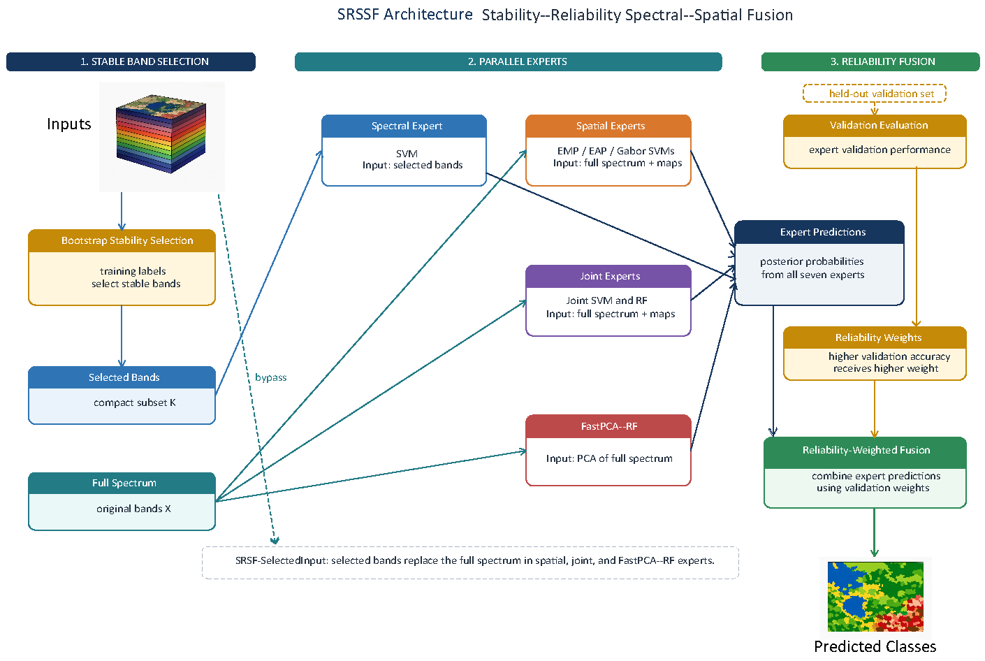
Figure 2.
Dataset split maps illustrating footprint-disjoint partitions into training, validation, and test sets. These visualizations confirm strict spatial exclusion and reproducibility of the evaluation protocol.
Figure 2.
Dataset split maps illustrating footprint-disjoint partitions into training, validation, and test sets. These visualizations confirm strict spatial exclusion and reproducibility of the evaluation protocol.
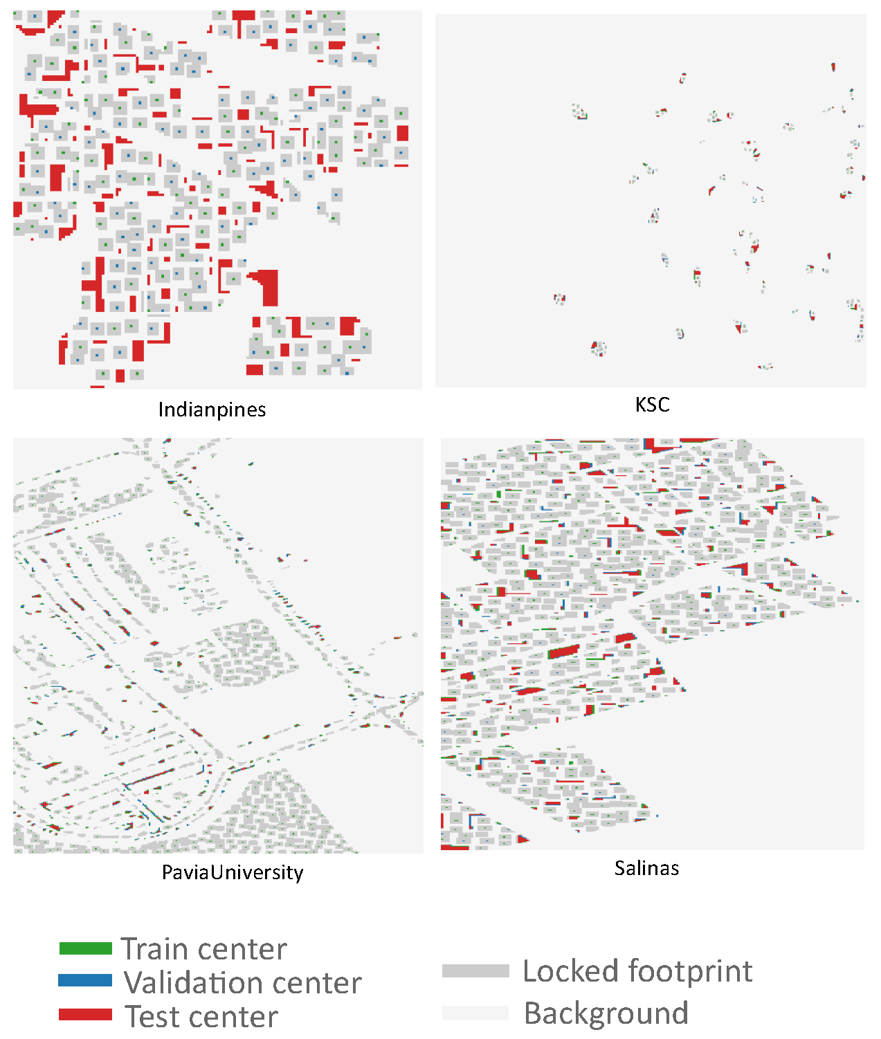
Figure 3.
Classification panels for Indian Pines under footprint-disjoint splits. Due to strict exclusion of neighboring pixels, maps appear fragmented and are not representative of visual quality. These panels are shown for completeness; quantitative metrics (OA/AA/Kappa) provide the valid basis for comparison.
Figure 3.
Classification panels for Indian Pines under footprint-disjoint splits. Due to strict exclusion of neighboring pixels, maps appear fragmented and are not representative of visual quality. These panels are shown for completeness; quantitative metrics (OA/AA/Kappa) provide the valid basis for comparison.
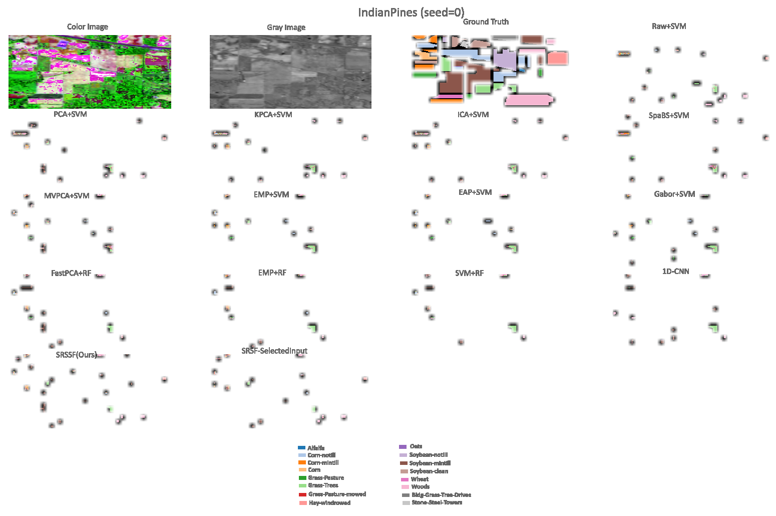
Figure 4.
Per-class accuracy heatmap highlighting strengths and residual confusions across vegetation types.
Figure 4.
Per-class accuracy heatmap highlighting strengths and residual confusions across vegetation types.
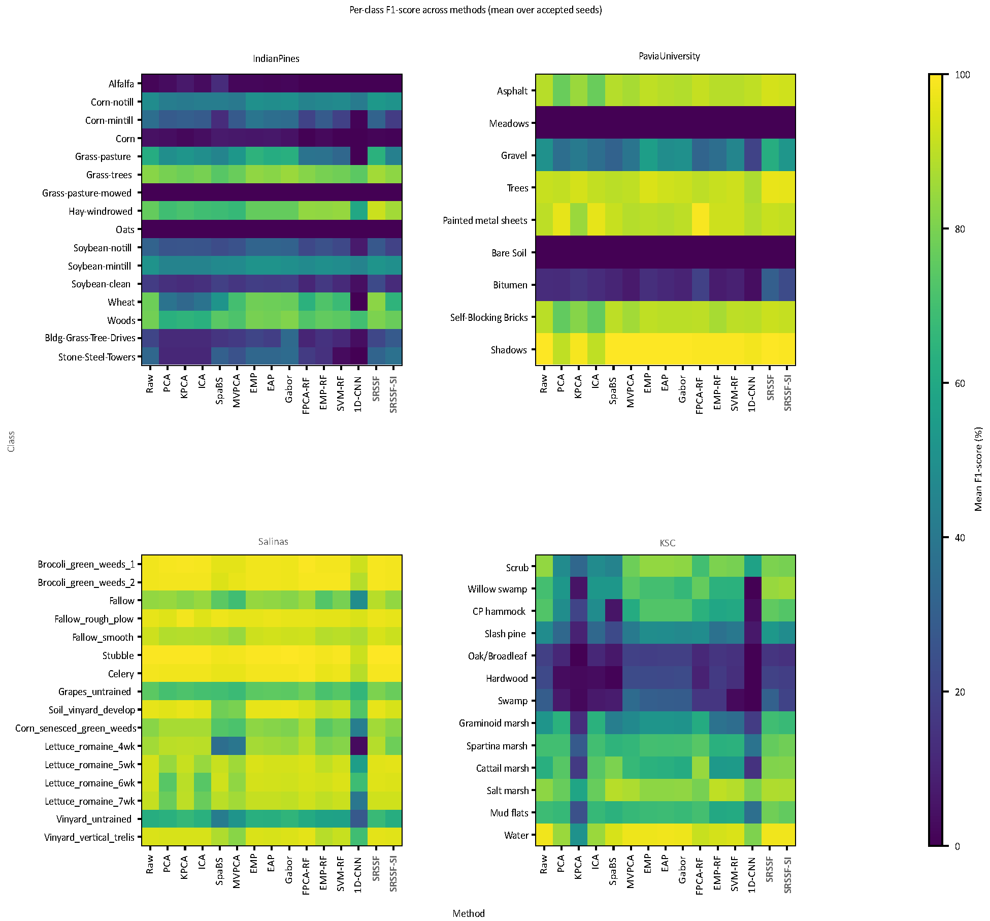
Figure 5.
Band stability analysis showing consistency of spectral importance across seeds and datasets.
Figure 5.
Band stability analysis showing consistency of spectral importance across seeds and datasets.
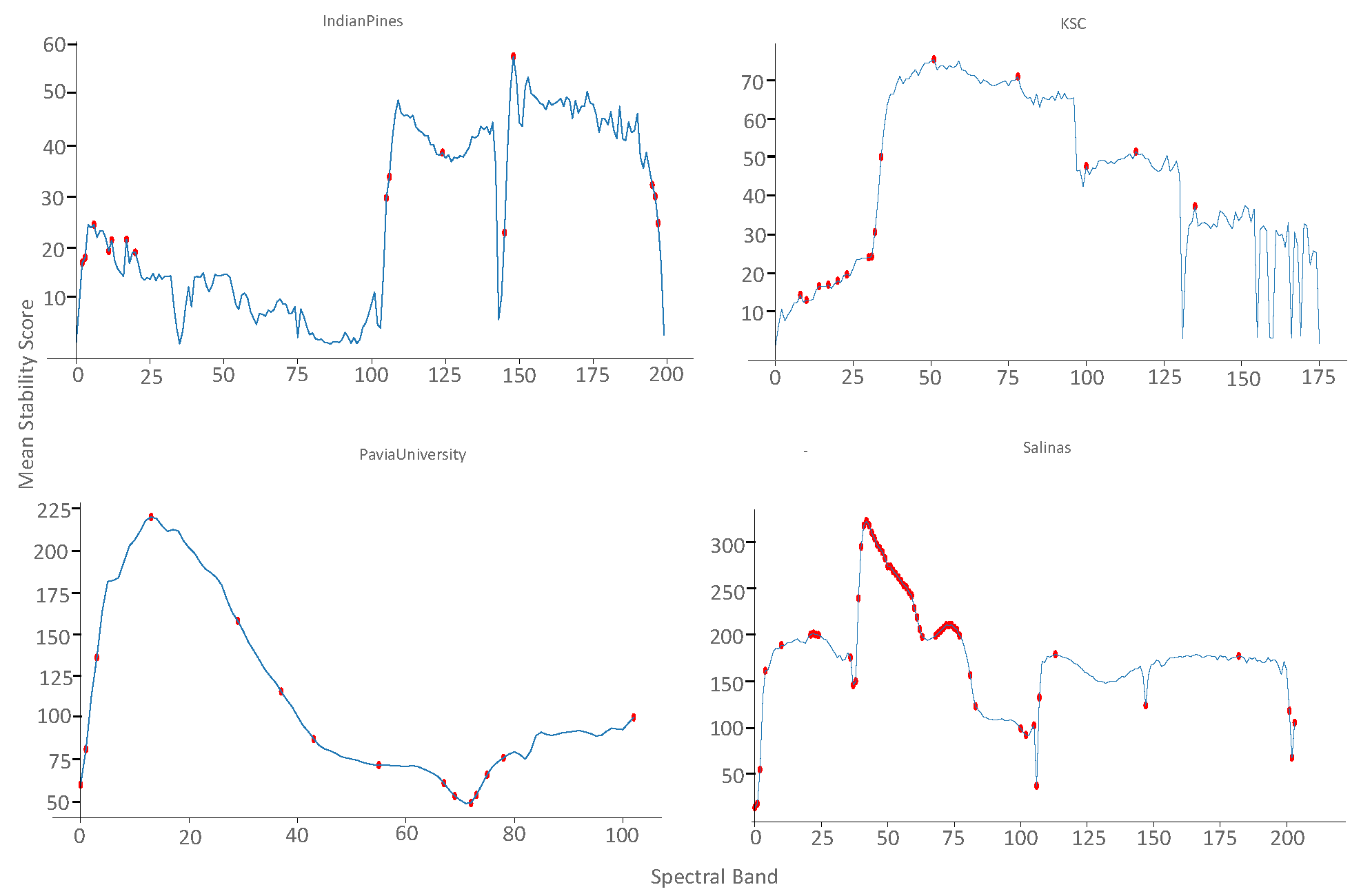
Figure 6.
Expert weight distribution comparing reliability-weighted fusion against domain knowledge.
Figure 6.
Expert weight distribution comparing reliability-weighted fusion against domain knowledge.
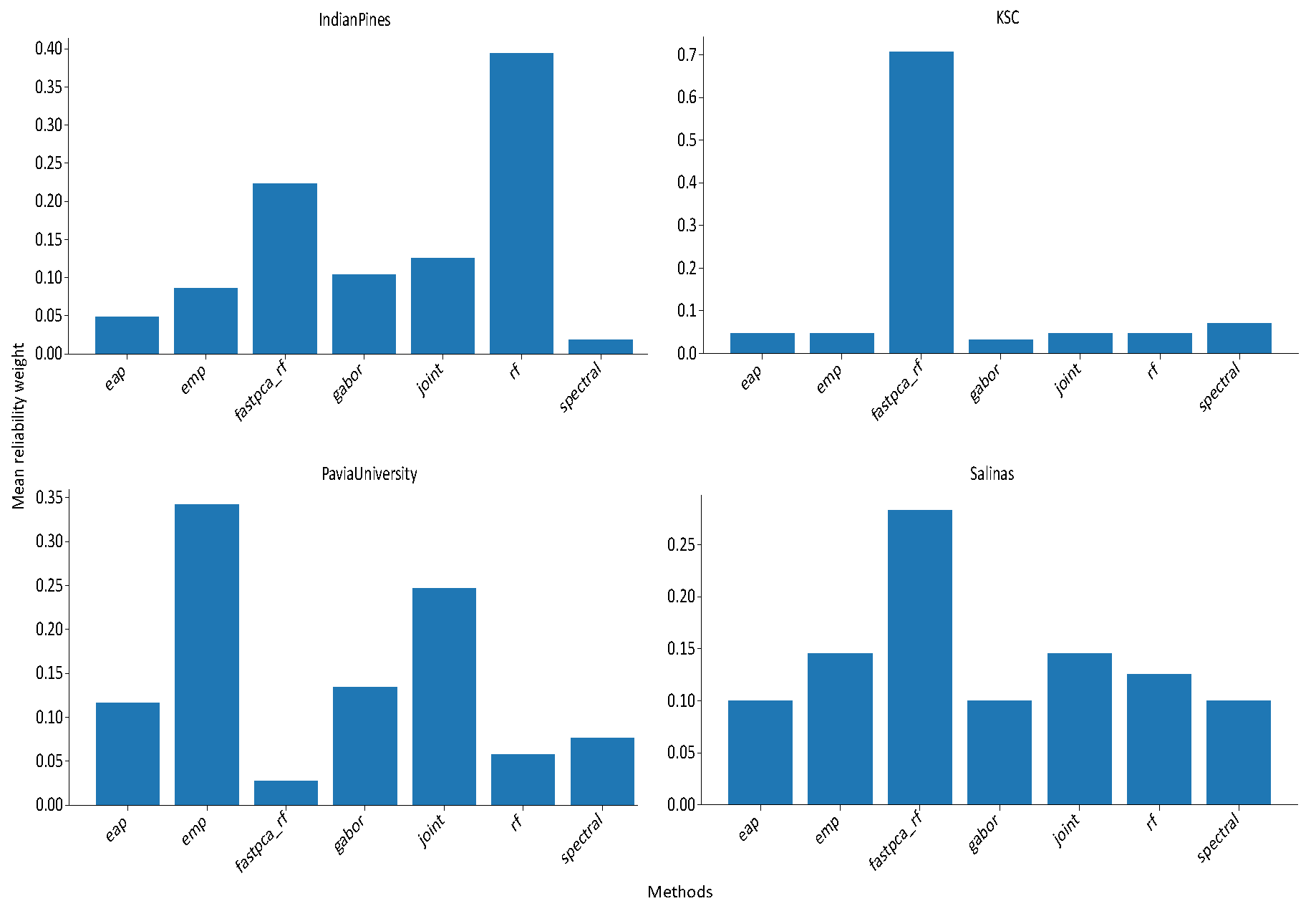
Figure 7.
SHAP heatmap illustrating per-class spectral contributions under reliability-weighted fusion.
Figure 7.
SHAP heatmap illustrating per-class spectral contributions under reliability-weighted fusion.
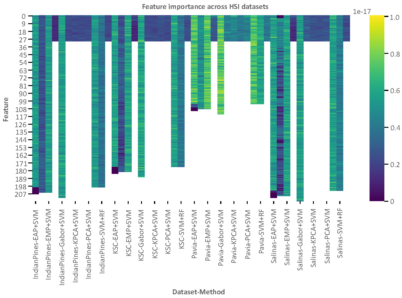

Table 1.
Per-class training/validation sampling fractions used before footprint locking. Effective counts after locking are reported per accepted seed (Section 3.2).
Table 1.
Per-class training/validation sampling fractions used before footprint locking. Effective counts after locking are reported per accepted seed (Section 3.2).
| Dataset | ||
| Indian Pines | 0.01 | 0.01 |
| Pavia University | 0.01 | 0.01 |
| Salinas | 0.01 | 0.01 |
| KSC | 0.01 | 0.01 |
Table 2.
Minimum required strict test-center count per dataset, used as an acceptance criterion for seed filtering.
Table 2.
Minimum required strict test-center count per dataset, used as an acceptance criterion for seed filtering.
| Dataset | |
| Indian Pines | 200 |
| Pavia University | 1500 |
| Salinas | 2000 |
| KSC | 100 |
Table 3.
Spatial patch size used for both spatial feature extraction and footprint-locking during data split.
Table 3.
Spatial patch size used for both spatial feature extraction and footprint-locking during data split.
| Dataset | Patch size p |
| Indian Pines | |
| Pavia University | |
| Salinas | |
| Kennedy Space Center (KSC) |
Table 4.
Main comparison: OA / AA / (%, mean ± std over 10 accepted seeds), all 15 methods. Best per dataset/metric in green, second best in bold.
Table 4.
Main comparison: OA / AA / (%, mean ± std over 10 accepted seeds), all 15 methods. Best per dataset/metric in green, second best in bold.
| Indian Pines | Pavia University | Salinas | KSC | |||||||||
| Method | OA | AA | OA | AA | OA | AA | OA | AA | ||||
| Raw+SVM | 52.88±3.81 | 42.62±3.79 | 46.44±4.30 | 86.13±2.20 | 63.26±4.74 | 81.36±2.61 | 88.04±1.75 | 90.19±1.83 | 87.02±1.93 | 68.32±3.06 | 61.74±2.43 | 65.05±3.37 |
| PCA+SVM | 44.58±3.45 | 34.22±2.57 | 36.53±3.88 | 78.26±1.73 | 56.19±2.98 | 71.06±2.27 | 86.02±1.80 | 86.48±2.24 | 84.79±2.04 | 60.28±3.91 | 49.72±3.52 | 55.84±4.34 |
| KPCA+SVM | 44.66±3.81 | 34.41±2.26 | 36.67±4.23 | 83.97±1.80 | 60.98±3.05 | 78.36±2.37 | 87.93±1.74 | 89.53±1.76 | 86.89±1.94 | 30.15±1.97 | 24.23±1.21 | 22.19±1.84 |
| ICA+SVM | 44.58±3.45 | 34.22±2.57 | 36.53±3.88 | 78.26±1.74 | 56.19±2.98 | 71.06±2.28 | 86.02±1.81 | 86.48±2.24 | 84.80±2.04 | 60.28±3.91 | 49.72±3.52 | 55.84±4.34 |
| SpaBS+SVM | 45.34±3.60 | 37.74±5.23 | 37.80±3.58 | 84.39±1.87 | 58.85±4.24 | 79.06±2.29 | 80.40±1.46 | 82.90±1.12 | 78.70±1.60 | 56.32±3.43 | 46.59±2.33 | 51.45±3.73 |
| MVPCA+SVM | 45.78±3.37 | 37.45±4.24 | 38.62±3.78 | 82.94±2.64 | 58.84±3.51 | 77.27±3.20 | 79.14±1.71 | 80.79±1.77 | 77.34±1.93 | 66.21±3.47 | 60.65±3.67 | 62.75±3.79 |
| EMP+SVM | 53.97 ±3.89 | 43.32±3.93 | 47.66 ±4.44 | 88.52±1.04 | 64.43 ±4.63 | 84.41±1.26 | 88.27±1.85 | 90.43±1.91 | 87.28±2.03 | 68.31±3.09 | 61.91±2.59 | 65.05±3.40 |
| EAP+SVM | 52.94±3.58 | 42.64±3.52 | 46.52±4.02 | 86.92±1.61 | 62.98±5.43 | 82.32±1.93 | 88.21±1.58 | 90.32±1.72 | 87.21±1.75 | 68.32±3.06 | 61.74±2.43 | 65.05±3.37 |
| Gabor+SVM | 53.84±3.97 | 43.33±4.03 | 47.51±4.47 | 86.17±1.85 | 62.39±5.00 | 81.39±2.26 | 87.98±1.54 | 90.08±1.73 | 86.97±1.68 | 67.49±3.58 | 61.32±2.80 | 64.16±3.91 |
| FastPCA+RF | 48.18±3.98 | 38.68±3.75 | 40.47±4.41 | 85.70±1.62 | 58.60±4.11 | 80.69±1.94 | 89.30 ±1.70 | 91.05 ±1.69 | 88.38 ±1.88 | 69.86±2.27 | 59.66±1.92 | 66.61±2.51 |
| EMP+RF | 50.06±4.39 | 40.44±4.46 | 42.96±4.64 | 84.54±2.42 | 60.04±4.41 | 79.27±2.88 | 84.55±2.52 | 86.86±2.69 | 83.23±2.78 | 62.27±2.61 | 54.35±2.47 | 58.29±2.81 |
| SVM+RF | 49.21±4.43 | 39.51±3.82 | 41.54±4.63 | 86.76±1.69 | 60.80±4.48 | 82.09±1.97 | 86.16±2.36 | 88.18±2.37 | 84.96±2.60 | 62.71±2.97 | 53.88±2.55 | 58.74±3.21 |
| 1D-CNN | 42.17±4.80 | 29.39±2.79 | 33.15±4.59 | 83.61±6.36 | 56.59±6.84 | 78.27±7.74 | 69.10±4.18 | 67.29±5.04 | 66.31±4.67 | 40.34±3.01 | 32.69±2.52 | 33.66±3.39 |
| SRSSF-SelectedInput | 52.23±5.32 | 43.77 ±2.38 | 45.03±5.75 | 90.82 ±1.13 | 63.73±4.91 | 87.37 ±1.51 | 88.26±2.15 | 90.04±2.14 | 87.25±2.37 | 75.06 ±3.41 | 65.55 ±3.00 | 72.42 ±3.72 |
| SRSSF(Ours) | 56.43±3.21 | 48.85±3.24 | 49.97±3.45 | 91.94±1.16 | 66.20±4.86 | 88.91±1.52 | 90.50±1.62 | 92.18±1.47 | 89.68±1.78 | 75.96±2.99 | 66.70±3.23 | 73.39±3.28 |
Table 5.
Few-shot OA (%, mean over 10 accepted seeds) vs. samples/class, all 15 methods. Best per dataset/budget in green.
Table 5.
Few-shot OA (%, mean over 10 accepted seeds) vs. samples/class, all 15 methods. Best per dataset/budget in green.
| Indian Pines | Pavia University | Salinas | KSC | |||||||||||||||||
| Method | 5 | 10 | 15 | 20 | 25 | 5 | 10 | 15 | 20 | 25 | 5 | 10 | 15 | 20 | 25 | 5 | 10 | 15 | 20 | 25 |
| Raw+SVM | 42.9 | 49.8 | 52.8 | 57.2 | 61.9 | 60.3 | 62.1 | 63.5 | 72.4 | 78.1 | 76.3 | 75.1 | 71.0 | 70.0 | 68.3 | 83.1 | 95.1 | 95.4 | 95.1 | 96.5 |
| PCA+SVM | 36.6 | 44.4 | 43.6 | 51.5 | 59.5 | 51.3 | 56.7 | 62.4 | 67.6 | 71.1 | 75.6 | 77.2 | 76.1 | 72.2 | 68.8 | 82.1 | 95.9 | 94.1 | 95.9 | 97.6 |
| KPCA+SVM | 37.3 | 45.0 | 44.4 | 52.7 | 60.1 | 59.2 | 61.5 | 68.7 | 73.4 | 77.6 | 76.0 | 78.2 | 74.8 | 73.0 | 70.4 | 39.8 | 78.9 | 72.4 | 78.9 | 89.8 |
| ICA+SVM | 36.6 | 44.4 | 43.6 | 51.5 | 59.5 | 51.3 | 56.7 | 62.4 | 67.6 | 71.1 | 75.6 | 77.2 | 76.1 | 72.2 | 68.8 | 82.1 | 95.9 | 94.1 | 95.9 | 97.6 |
| SpaBS+SVM | 34.7 | 47.6 | 52.3 | 62.2 | 69.4 | 59.0 | 56.5 | 60.2 | 66.5 | 73.6 | 72.7 | 72.9 | 70.3 | 70.5 | 66.3 | 68.4 | 91.5 | 92.6 | 91.5 | 95.6 |
| MVPCA+SVM | 35.2 | 40.2 | 42.9 | 50.7 | 56.0 | 57.9 | 60.0 | 64.4 | 69.5 | 72.9 | 69.0 | 70.8 | 67.0 | 65.7 | 63.5 | 80.1 | 94.1 | 95.0 | 94.1 | 96.8 |
| EMP+SVM | 43.4 | 50.3 | 53.9 | 57.9 | 63.0 | 61.4 | 64.4 | 67.0 | 75.6 | 81.3 | 76.4 | 75.3 | 71.3 | 70.1 | 68.0 | 83.3 | 94.6 | 95.5 | 94.6 | 96.3 |
| EAP+SVM | 42.9 | 49.8 | 52.7 | 57.2 | 61.5 | 60.8 | 62.8 | 64.2 | 73.2 | 78.5 | 76.2 | 75.2 | 70.9 | 69.6 | 68.1 | 83.1 | 95.1 | 95.4 | 95.1 | 96.5 |
| Gabor+SVM | 44.4 | 50.3 | 53.3 | 57.4 | 61.5 | 60.9 | 62.8 | 65.5 | 71.7 | 78.1 | 76.0 | 75.7 | 71.6 | 70.4 | 68.8 | 83.2 | 94.9 | 95.1 | 94.9 | 96.5 |
| FastPCA+RF | 40.4 | 50.0 | 48.8 | 58.3 | 66.4 | 61.8 | 64.6 | 67.9 | 74.0 | 76.5 | 78.7 | 79.5 | 76.4 | 74.0 | 70.8 | 86.0 | 95.7 | 94.2 | 95.7 | 97.6 |
| EMP+RF | 42.7 | 52.4 | 55.6 | 59.7 | 69.4 | 58.1 | 57.1 | 56.6 | 61.5 | 65.9 | 74.5 | 73.4 | 68.9 | 67.7 | 64.6 | 79.8 | 95.5 | 96.1 | 95.5 | 96.1 |
| SVM+RF | 42.7 | 53.7 | 57.3 | 61.5 | 71.0 | 57.8 | 58.4 | 58.9 | 66.2 | 72.2 | 75.3 | 73.6 | 68.9 | 68.3 | 65.2 | 81.3 | 96.3 | 96.7 | 96.3 | 99.1 |
| 1D-CNN | 34.0 | 49.3 | 51.9 | 61.4 | 67.7 | 50.3 | 54.0 | 55.3 | 63.3 | 61.4 | 61.0 | 60.0 | 60.8 | 59.6 | 52.0 | 66.6 | 90.6 | 67.1 | 90.6 | 86.2 |
| SRSSF-SelectedInput | 49.2 | 54.7 | 58.0 | 59.9 | 67.8 | 67.5 | 72.9 | 77.1 | 80.4 | 82.4 | 79.8 | 78.3 | 74.5 | 74.2 | 72.7 | 87.7 | 96.0 | 97.7 | 96.0 | 97.8 |
| SRSSF(Ours) | 50.6 | 56.3 | 58.9 | 63.4 | 66.3 | 68.2 | 73.7 | 78.3 | 80.8 | 83.7 | 79.7 | 79.5 | 77.1 | 75.7 | 75.5 | 88.3 | 96.4 | 97.9 | 96.4 | 97.9 |
Table 6.
Efficiency (mean over 10 seeds, averaged across datasets, Best in green.)
| Method | Fit (s) | Infer (s) | Mem. (MB) |
| Raw+SVM | 0.11 | <0.001 | 4.5 |
| PCA+SVM | 0.14 | <0.001 | 1.1 |
| KPCA+SVM | 0.14 | <0.001 | 1.1 |
| ICA+SVM | 0.15 | <0.001 | 1.1 |
| SpaBS+SVM | 0.05 | <0.001 | 0.9 |
| MVPCA+SVM | 0.08 | <0.001 | 1.1 |
| EMP+SVM | 0.13 | <0.001 | 3.7 |
| EAP+SVM | 0.14 | <0.001 | 3.9 |
| Gabor+SVM | 0.13 | <0.001 | 4.0 |
| FastPCA+RF | 1.28 | <0.001 | 0.9 |
| EMP+RF | 1.40 | <0.001 | 1.9 |
| SVM+RF | 1.70 | <0.001 | 3.7 |
| 1D-CNN | 6.9 | <0.001 | 3.9 |
| SRSSF-SelectedInput | 5.9 | 0.6 | 5.1 |
| SRSSF (Ours) | 6.4 | 0.9 | 15.0 |
Table 7.
Ablation OA (%, mean ± std over 10 seeds, Best in green).
| Configuration | Indian Pines | Pavia University | Salinas | KSC |
| RawSVM | 52.88±3.81 | 86.13±2.20 | 88.04±1.75 | 68.32±3.06 |
| Spectral-Only+Sel. | 43.62±4.79 | 82.57±1.78 | 84.41±3.14 | 66.63±3.47 |
| Fusion, No Band Sel. | 56.89±3.18 | 91.97±1.16 | 90.55±1.60 | 75.98±3.13 |
| Uniform Fusion | 56.09±4.07 | 91.68±1.02 | 90.26±1.63 | 75.50±3.65 |
| SRSSF-SelectedInput | 52.23±5.32 | 90.82±1.13 | 88.26±2.15 | 75.06±3.41 |
| SRSSF(Ours) | 56.43±3.21 | 91.94±1.16 | 90.50±1.62 | 75.96±2.99 |
Disclaimer/Publisher’s Note: The statements, opinions and data contained in all publications are solely those of the individual author(s) and contributor(s) and not of MDPI and/or the editor(s). MDPI and/or the editor(s) disclaim responsibility for any injury to people or property resulting from any ideas, methods, instructions or products referred to in the content. |
© 2026 by the authors. Licensee MDPI, Basel, Switzerland. This article is an open access article distributed under the terms and conditions of the Creative Commons Attribution (CC BY) license (http://creativecommons.org/licenses/by/4.0/).
Copyright: This open access article is published under a Creative Commons CC BY 4.0 license, which permit the free download, distribution, and reuse, provided that the author and preprint are cited in any reuse.