

Submitted:
17 September 2026
Posted:
24 September 2026
You are already at the latest version
Abstract
Periodic condition assessment of Natura 2000 (N2K)—the EU's network of protected areas under the Habitats Directive—is legally mandated but cannot be sustained at the required spatial scale through field survey alone. We introduce a multi-country Leave-One-Park-Out (LOPO) evaluation framework for binary per-habitat segmentation of N2K grasslands from Sentinel-2 multitemporal imagery, implemented using a parameter-efficient adaptation of the Prithvi-EO-2.0 geospatial foundation model. The framework spans four protected areas across Spain, Portugal, and France and three European biogeographic regions. Low-Rank Adaptation (LoRA) adapters (r=16, 6.3 M trainable parameters) fine-tune the frozen ViT-L backbone alongside a UPerNet decoder, ingesting three stochastically sampled monthly composites per training iteration. LOPO evaluation on three habitat configurations—semi-natural calcareous and Nardus grasslands (6210+6230), lowland and mountain hay meadows (6510+6520), and thermo-Mediterranean grasslands (6220)—assesses cross-park generalisation across ecologically distinct parks, with mean LOPO mIoU of 45.8% for 6210+6230 and 52.2% for 6510+6520 following a controlled data-expansion experiment that increases habitat-positive supervision by a factor of 25.3. A same-architecture within-park baseline inflates mean mIoU by 14.0 pp, directly quantifying the optimistic bias of conventional single-site evaluation.
Keywords:
remote sensing
; habitat mapping
; Natura 2000
; foundation model
; Prithvi-EO-2.0
; Sentinel 2
; transfer learning
; multitemporal imagery
; conservation monitoring
1. Introduction
The Natura 2000 (N2K) network is the world’s largest coordinated system of protected areas, covering more than 18% of European land surface and encompassing over 230 officially classified natural habitat types [1]. Under the EU Habitats Directive (92/43/EEC), member states are legally required to carry out periodic condition assessments for each protected site, a task that still relies almost entirely on in-situ field survey. At the spatial scale demanded by conservation policy this is increasingly impractical: mapping habitats at the required resolution using field work alone demands survey effort and budgets that most agencies cannot sustain, so that official habitat maps are systematically outdated and the ecological trends they are intended to capture go undetected. The monitoring gap is most acute for fine-grained semi-natural grassland mosaics—calcareous and thermo-Mediterranean grasslands, hay meadows, and the herbaceous swards of Mediterranean dehesa landscapes—whose dynamic seasonal phenology is impractical to survey in the field at the scale at which it occurs.
Earth observation offers a scalable alternative. The Sentinel-2 constellation acquires free, open-access multispectral imagery at 10 m spatial resolution with an approximately five-day revisit interval [2], and its high acquisition frequency turns the archive into a temporal record in which each location is observed as a time series rather than a single snapshot. This temporal dimension is decisive for habitat discrimination: many N2K grassland types are spectrally indistinguishable on any single date and become separable only through their seasonal trajectory [3]. Therophytic annual grasslands of southern Europe, for instance, reach peak NDVI in spring and approach bare-soil values in summer and winter [4], so that a classifier must observe both the spring growth peak and the dormant season to separate habitat from background reliably. As detailed in Section 2, this temporal specificity is shared across the habitat types targeted here, and no single acquisition date captures the full ecological signal.
Despite the maturity of dense satellite time series and deep learning, habitat mapping at the directive level remains an open problem for two reasons. First, conventional supervised approaches—gradient-boosted trees or convolutional networks trained from random initialisation—require large labelled datasets that are costly to produce and are typically confined to a single area and a restricted set of classes [5,6,7]. Second, and more fundamentally, models trained and validated within the same site do not establish cross-site generalisation: a classifier that performs well at one park may merely have memorised local spectral idiosyncrasies rather than learned transferable ecological representations. Addressing this second point requires both an evaluation protocol that holds out entire sites and a model whose representations are not learned from the target site alone.
Geospatial Foundation Models (GFMs) trained on large-scale satellite archives offer such representations. By learning general descriptions of Earth-surface dynamics from millions of unlabelled time series, GFMs such as Prithvi-EO-2.0 [8] encode a broad prior over how landscapes vary spectrally and temporally; Prithvi-EO-2.0 was pretrained on 4.2 million global samples from the Harmonized Landsat and Sentinel-2 (HLS) archive at 30 m resolution using a masked-autoencoder framework with explicit spatiotemporal attention. Despite the rapid proliferation of GFMs [9,10,11,12,13], no validated adaptation with rigorous cross-site generalisation testing for fine-grained N2K habitat classification has been reported. Binary per-habitat segmentation—one model per N2K type predicting presence or absence—is the natural unit of analysis for directive-level monitoring: it decouples fine-grained between-class discrimination from the cross-site generalisation question and allows each habitat model to be updated independently as new field data become available.
This paper addresses that gap with three contributions. First, a multi-country Leave-One-Park-Out (LOPO) protocol for binary per-habitat N2K segmentation that holds out entire protected areas at evaluation time and directly quantifies the optimistic bias of conventional within-park validation. Second, controlled data-expansion experiments that identify absolute supervision volume and ecological proximity of the auxiliary pool as candidate determinants of cross-park detection performance within the architectures evaluated here. Third, a parameter-efficient adaptation of Prithvi-EO-2.0 (LoRA , UPerNet decoder) as the backbone evaluated under this protocol, with architecture baselines contextualising the performance of the Prithvi-based adaptation relative to generic ImageNet pretraining and random initialisation. The corresponding architecture, protocol, and quantitative results are presented in Section 4 and Section 5.
The remainder of this paper is organised as follows. Section 2 reviews related work. Section 3 describes the study areas, Sentinel-2 data, and habitat labels. Section 4 presents the proposed architecture, LOPO protocol, and training configuration. Section 5 reports LOPO results per habitat type. Section 6 discusses cross-park generalisation findings. Section 7 concludes.
2. Background and Related Work
2.1. Target Grassland Habitats and Their Phenology
The habitats evaluated in this paper represent three ecologically distinct grassland types, all Habitats of Community Interest (HCIs) listed under Annex I of the Habitats Directive (92/43/EEC) [14,15,16]. Semi-natural dry grasslands and scrubland facies on calcareous substrates (HCI 6210) support exceptionally rich plant communities in the Atlantic and Alpine biogeographic regions [15,17]. Nardus-dominated grasslands on siliceous soils (HCI 6230) constitute another species-rich grassland type within these regions [16,18]. Both habitats are particularly vulnerable to land-use change and vegetation succession [17,19]. Grazing abandonment may lead to shrub encroachment and changes in habitat composition and spatial distribution [18,19].
Lowland and mountain hay meadows (HCI 6510 and HCI 6520) follow a distinct seasonal cycle [3,20]. Vegetation growth peaks in spring, whereas senescence begins shortly after mowing [21,22]. Seasonal changes in vegetation growth and senescence create a characteristic temporal profile in satellite image time series [3,20]. In addition, their fragmented occurrence and often limited extent increase the difficulty of accurate habitat delineation [17]. Changes in mowing regimes and fertilisation practices may further alter their ecological characteristics and spatial extent [21,23].
Thermo-Mediterranean grasslands (HCI 6220) are common in the dehesa landscapes of southwestern Iberia [24,25]. Vegetation productivity peaks in spring and declines during the summer dormant period [4,24]. This contrast in principle makes HCI 6220 detectable by a multitemporal classifier, but wide floristic and structural variation among grazing and management regimes reduces the distinctiveness of its spectral signature and demands training data that span this variation [4,7]. Differences in phenology, vegetation composition, management history, and spatial configuration create substantial ecological variability among protected areas [7,17]. Ecological variability at this scale provides a useful basis for assessing the ability of geospatial foundation models to generalise under different ecological conditions [8,26,27].
Grasslands are the exclusive focus of this evaluation because they combine the highest EU-wide conservation urgency among Annex I habitat types with the greatest spectral ambiguity: unlike structurally distinct classes such as closed-canopy forest or open water, which are separable from a single acquisition date, the grassland types evaluated here are phenologically driven and require dense multitemporal observation to discriminate reliably—making them both the most consequential and the most technically demanding test of the proposed framework.
2.2. Remote Sensing for N2K Habitat Monitoring
The application of satellite imagery to N2K condition assessment has a substantial history [6]. Early efforts relied on multispectral classification with random forests, support vector machines, and gradient-boosted trees applied to single-date Sentinel-2 or Landsat acquisitions [5]. These approaches achieve satisfactory accuracy on structurally distinct classes such as closed-canopy forest and open water but consistently fail to resolve the fine-grained grassland and heath subtypes defined by the Habitats Directive, which are spectrally indistinguishable at any single acquisition date and require explicit temporal context to differentiate [3,5].
Recent work has begun applying convolutional and transformer deep-learning architectures to N2K classification at the directive level. Díaz-Ireland et al. (2024) [7] evaluated several CNN and transformer architectures for protected grassland classification in the Castilla y León region (Spain) using Sentinel-2 imagery, and is the direct predecessor to the present work. All architectures in that study were trained from scratch or with ImageNet pretraining on a single geographic region and were not evaluated for cross-site generalisation; this paper extends the line of work by introducing a foundation-model backbone and a strict leave-one-park-out evaluation across multiple countries.
2.3. Geospatial Foundation Models
GFMs pretrained on global satellite archives represent a qualitative advance over task-specific architectures. Prithvi-EO-2.0 [8] encodes spatiotemporal context through sinusoidal year, day-of-year, and location embeddings and outperforms six competing GFMs on the GEO-Bench benchmark. TerraMind [12], developed by IBM and ESA’s -lab, extends the paradigm to any-to-any generative multimodal reasoning across Sentinel-2, SAR, and DEM inputs. Additional GFMs targeting different representation strategies include TESSERA [9], AlphaEarth [10], and Earth Embeddings [11]. None of these models has been evaluated under a cross-site, leave-one-region-out protocol for fine-grained Habitats Directive classification: reported benchmarks assess either global, coarse land-cover tasks (GEO-Bench) or within-region accuracy, neither of which quantifies the site-memorisation risk this paper’s LOPO protocol is designed to expose (Section 6).
The ecological applicability of GFMs was assessed by Mahlasi et al. [13], who fine-tuned Prithvi-EO-2.0 and TerraMind on forest functional trait estimation, LULC mapping, and peatland detection, with both GFMs consistently outperforming a ResNet-101 baseline. That evaluation, like the GEO-Bench results above, is within-region: it establishes that GFM fine-tuning outperforms non-pretrained baselines on ecological tasks, but does not test whether the resulting model generalises to protected areas outside the training distribution—the specific question this paper’s LOPO protocol answers for N2K grassland habitats.
2.4. Parameter-Efficient Fine-Tuning
Adapting a frozen foundation-model backbone such as Prithvi-EO-2.0 to a downstream segmentation task, without retraining its hundreds of millions of pretrained weights, is the role of parameter-efficient fine-tuning (PEFT). Low-Rank Adaptation (LoRA) [28] injects rank-decomposed weight residuals into transformer attention layers, enabling adaptation of large pretrained models with a fraction of the original parameter count. In the context of GFMs for ecological mapping, PEFT is the natural choice: full fine-tuning of a 300M-parameter backbone on a domain-specific dataset risks catastrophic forgetting of the global EO representations that provide cross-site generalisation, and PEFT side-steps that risk by construction.
3. Study Area and Data
3.1. Study Areas
The study encompasses N2K protected areas across Spain, Portugal, and France, spanning three of the nine European biogeographic regions defined under the Habitats Directive—Atlantic, Alpine, and Mediterranean (Table 1). Four primary parks provide training and validation data: Ordesa y Monte Perdido and Sierra de Aracena (Spain), Peneda-Gerês (Portugal), and Causses du Quercy (France). For the data expansion experiments, three large-area tile regions covering central and southern Catalonia, contributing 5,449 training tiles, are incorporated as additional training data for hay meadow habitats (HCI 6510+6520; multi-fold experiment of Section 5.2). For the analogous expansion experiment on calcareous grasslands (HCI 6210+6230; Section 5.3), two large-area Catalonian tile regions and six Aragon tile regions are used as auxiliary training-only data, contributing a further 2,628 and 4,340 training tiles respectively (the full per-park composition is detailed in Section 3.4).
The four primary parks collectively span 369,621 ha (Table 1): Gerês sits in the Atlantic region, Ordesa in the Alpine region (which contains the Pyrenees under the EEA classification), and Aracena and the southern portion of Quercy in the Mediterranean region. Shannon diversity indices range from at Gerês (10 habitat types, dominated by a single woodland class) to at Quercy (23 habitat types, dominated by calcareous grasslands), reflecting the broad ecological range of the training portfolio. The geographic distribution of the four parks across the three biogeographic regions is shown in Figure 1; their habitat-tile coverage is shown separately in Figure 3.
3.2. Sentinel-2 Time Series
Sentinel-2 Level-2A surface reflectance imagery was acquired for all study areas. Six spectral bands were selected to match the HLS bands used during Prithvi-EO-2.0 pretraining: B02 (blue, 490 nm), B03 (green, 560 nm), B04 (red, 665 nm), B8A (narrow NIR, 865 nm), B11 (SWIR1, 1610 nm), and B12 (SWIR2, 2190 nm), all resampled to 10 m spatial resolution [2].
The temporal series encompasses three acquisition years (2018, 2024, and 2025), yielding 36 monthly best-available-pixel (BAP) composites per site stored as a 4D Zarr datacube of shape . Each composite selects cloud-free, low-aerosol observations within a 30-day window centred on the target month. The three acquisition years span the heterogeneous label years of the four primary parks (Table 1: Ordesa 2018, Aracena 2024; Gerês and Quercy both have label year 2017), so a single uniform 36-month datacube schema can be applied to every park while preserving each park’s paired acquisition year as the supervisory window: for Ordesa and Aracena, the paired acquisition year matches the inventory year directly; for Gerês and Quercy, the 2017 inventories are paired with the nearest available 2018 Sentinel-2 archive. At training time, however, only the 12-month slice corresponding to the relevant park’s paired acquisition year is exposed to the sampler (Section 4.4); the remaining 24 months are retained in the archive for the change-detection and temporal-robustness analyses that extend this dataset beyond the present paper. In particular, the 2025 slice carries no habitat labels for the four primary parks and is therefore never used in their training or validation folds; it serves only as a production-inference year for those parks. (The Andalucía and Catalunya auxiliary regions used in the data-expansion experiments of Section 5 carry their own 2024/2025 habitat inventories and are used as training-only data—see Table 3.) Subsequent years (2026 onward) can be processed identically as they become available for the primary parks, since production inference requires no labels. The label years actually used for training and validation span 2017–2024 across the four primary parks (Table 1), not a single contiguous window; the 2025 production-inference pass (Section 5.7) demonstrates operational applicability rather than temporal generalisation, since no 2025 ground truth exists to validate against, and robustness to inter-annual variability beyond the years used is not directly tested (Section 6.4).
3.3. Habitat Labels
Ground-truth habitat polygons were obtained from the official N2K inventory databases of each country: Spain (MITERD, https://www.miteco.gob.es, accessed on 30 May 2026), Portugal (ICNF, https://www.icnf.pt, accessed on 30 May 2026), and France (MNHN/INPN, https://inpn.mnhn.fr, accessed on 30 May 2026). Polygons are delineated according to Annex I of the Habitats Directive (92/43/EEC).
For each target habitat type a binary label map is derived: pixels belonging to that habitat are assigned class 1 and all other labelled pixels are assigned class 0. The data pipeline currently supports six such binary configurations; this paper evaluates the three for which at least two parks hold documented occurrences, so that a Leave-One-Park-Out protocol is feasible (Table 2). The remaining three configurations (HCI 6140, 6170, 6310) have label sets prepared but are present in only a single park each, placing them outside the cross-park scope of this paper (Section 6.4).
3.4. Dataset Composition and LOPO Splits
Each park’s raster extent was subdivided into 224×224 pixel tiles (2.24 km × 2.24 km) with a stride of 112 pixels (50% overlap) to prevent edge-zone information loss. Tiles with more than 1% no-data pixels were excluded. The end-to-end data pipeline is illustrated in Figure 2: starting from the 4D Zarr datacube assembled per park, the pipeline selects the six HLS-compatible Sentinel-2 bands, rasterises the Natura 2000 habitat polygons into binary per-habitat label maps, extracts the overlapping 224×224 px tiles described above, stochastically samples three timesteps per training tile (Section 4.4), and assembles the resulting tensors into training batches. The resulting tile coverage over a representative study area is shown in Figure 3.
Figure 2.
End-to-end data pipeline. Starting from the 4D Zarr datacube (), the pipeline selects the six HLS-compatible bands, extracts overlapping 224×224 px tiles at 112 px stride, samples three timesteps per tile, and assembles batches for training.
Figure 2.
End-to-end data pipeline. Starting from the 4D Zarr datacube (), the pipeline selects the six HLS-compatible bands, extracts overlapping 224×224 px tiles at 112 px stride, samples three timesteps per tile, and assembles batches for training.
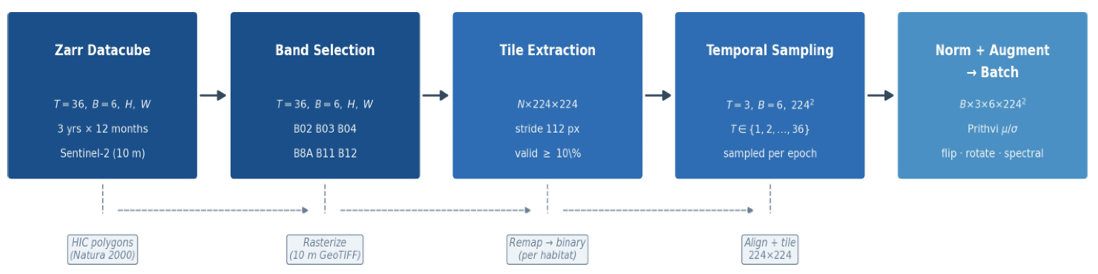
Figure 3.
Tile sampling across the study parks and auxiliary training regions. Each panel shows the 224×224 px tiles (2240 m × 2240 m at 10 m resolution) extracted with 112 px stride (50% overlap) overlaid on Esri WorldImagery. Habitat classes are colour-coded (see legend); these are the relevant habitat grasslands in the study area evaluated under the LOPO protocol (Table 2). The Aragón–Catalunya region (northeast Spain) is shown with a single merged study-region boundary; the individual park panels are shown without boundary overlays. Tiles with more than 1% no-data pixels per band were excluded (see Section 3.4).
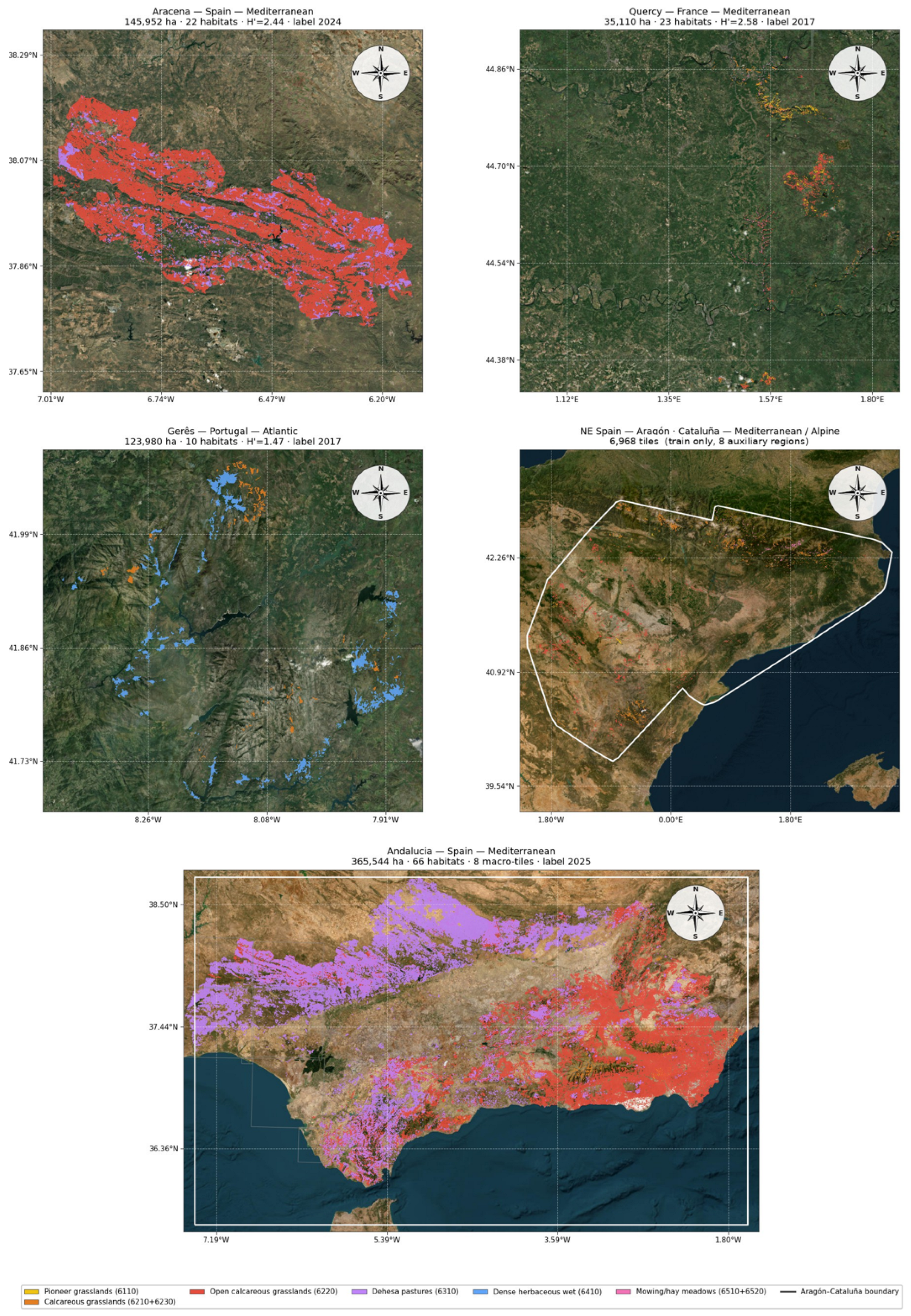
Table 3 reports the tile counts, positive pixel fractions, and absolute positive-pixel counts for each park–habitat combination, together with per-configuration totals. The absolute counts are computed directly from the rasterised binary label maps (excluding ignore pixels outside the park boundary), and are the metric the loss actually sees during training. Class imbalance varies widely: 6220 at Aracena is habitat-dominated (73.0%), whereas base 6510+6520 at Ordesa is almost entirely background (0.3%). More importantly, the absolute positive supervision varies by more than two orders of magnitude across configurations—from 52 K positive pixels for the base 6510+6520 configuration to over 10 M for 6220—which appears to be a major determinant of which habitats are detected in the experiments of Section 5 (see also Section 6.4). Imbalance is addressed through a weighted random tile sampler (max oversample ratio ) and an imbalance-aware composite loss, described in Section 4.5, but neither mechanism manufactures positive supervision where the underlying labelled set provides almost none.

Table 3.
Dataset composition per habitat type and park. Pos. pixels = absolute habitat-positive pixel count in the binary label map (the supervision the loss sees). Catalunya, Aragon, and Andalucía rows are auxiliary training-only regions with no held-out LOPO fold; their use in each expansion experiment is detailed in Section 5. Valid-pixel totals do not scale linearly with nominal tile area (Tiles × ) for two reasons: tiles exceeding the 1% per-band NoData threshold (Section 3.4) are excluded entirely, and pixels outside the irregular park boundary within an otherwise-valid tile are masked as ignore pixels and excluded from both the denominator and the positive-pixel counts above.
| Habitat | Park | Tiles | Pos. pixel % | Pos. pixels |
|---|---|---|---|---|
| 6210+6230 | Gerês | 660 | 1.4 | 91,524 |
| Ordesa | 354 | 24.8 | 865,123 | |
| Quercy | 423 | 7.2 | 178,882 | |
| Catalunya (train only, 2 regions) | 2,628 | 11.3 | 2,173,432 | |
| Aragon (train only, 6 regions) | 4,340 | 12.9 | 2,970,374 | |
| Total (+Cat +Aragon) | 8,405 | 11.5 | 6,279,335 | |
| 6510+6520 | Ordesa | 354 | 0.3 | 9,544 |
| Quercy | 423 | 1.7 | 42,440 | |
| Subtotal (base) | 777 | 0.9 | 51,984 | |
| Catalunya (train only) | 5,449 | 4.4 | 1,265,037 | |
| Total (+Cat.) | 6,226 | 3.4 | 1,317,021 | |
| 6220 | Aracena | 1,612 | 73.0 | 10,344,480 |
| Quercy | 423 | 6.7 | 166,326 | |
| Subtotal (base) | 2,035 | 63.1 | 10,510,806 | |
| Andalucía (train only, 2 regions) | 2,888 | 30.0 | 8,619,726 | |
| Total (+Andalucía) | 4,923 | 44.0 | 19,130,532 |
4. Methods
4.1. Architecture Overview
The proposed architecture is a parameter-efficient segmentation framework built around the frozen Prithvi-EO-2.0 backbone. Four trainable components are added: LoRA adapters injected into the backbone attention and feed-forward layers, a UPerNet decoder [29] that fuses multi-scale backbone feature maps and reconstructs the full-resolution segmentation map, a seasonal encoder that concatenates an explicit day-of-year embedding at the decoder input (retained for fidelity to the trained checkpoints but shown in Section 4.3 to be largely redundant with the backbone’s own temporal representation), and a FiLM park-conditioning module (Section 4.2). Table S1 and Figure 4 summarise the architecture. As shown in the figure, the model processes each input left to right: three stochastically sampled Sentinel-2 timesteps enter a Conv3D input embedding; the frozen Prithvi-EO-2.0 backbone with LoRA adapters extracts multi-scale features; a Feature Pyramid Network (FPN) neck fuses these features across scales; the UPerNet decoder combines the fused features with the seasonal encoder and FiLM park-conditioning signals; and a final convolution head produces the binary habitat mask.
4.2. Backbone and Parameter-Efficient Adaptation
The backbone is Prithvi-EO-2.0 [8], a Vision Transformer Large (ViT-L) pretrained on global samples from NASA’s Harmonized Landsat and Sentinel-2 (HLS) archive using a masked autoencoder objective with explicit spatiotemporal attention. Backbone weights are kept strictly frozen throughout fine-tuning; task-specific learning is confined to the LoRA adapters and trainable decoder-side components.
Pretraining used HLS imagery at 30 m resolution; our Sentinel-2 inputs are represented on a 10 m analysis grid. As described in Section 3.2, B8A, B11, and B12 are resampled to 10 m, while B02, B03, and B04 are natively available at 10 m. No resolution-adaptation step is applied to compensate for the mismatch with pretraining: the patch size and positional-embedding grid are unchanged, and the resulting six-band 10 m inputs are passed directly to Prithvi without downsampling to the 30 m HLS pretraining resolution, so each patch covers a smaller physical footprint at inference than during pretraining. The only interpolation in the pipeline is on the output side, where the decoder’s logits are bilinearly upsampled to the full tile resolution; whether an input-side adaptation (resampling, patch-size change, or positional-embedding interpolation) would improve on this is discussed as an open question in Section 7.
LoRA modules [28] are injected into the combined query-key-value projection, the attention output projection, and both feed-forward layers of every transformer block (target modules qkv, proj, fc1, fc2), introducing rank-decomposed residual corrections , where , , and rank . LoRA parameters are trained at a learning rate one order of magnitude lower than the decoder ( vs. ). Figure 5 illustrates the low-rank decomposition mechanism and the four injection points.
The UPerNet decoder [29] receives multi-scale feature maps from the backbone via a Feature Pyramid Network (FPN) with 256 channels, fuses them through Pyramid Pooling Module (PPM) context aggregation, and reconstructs the full-resolution segmentation map via successive upsampling.
A FiLM park conditioning module injects a learned site-level embedding into the decoder feature maps via affine scale-and-shift transformations. Each park is assigned an embedding of dimension 32, which modulates a 64-channel decoder layer. The FiLM module adds only ∼4 K trainable parameters and is included in every LOPO model because it forms part of the production deployment architecture: a similar, more advanced architecture is used for deployment, where the inference park is generally observed during training and per-park conditioning is operationally useful, so this module is retained here for fidelity to that design rather than introduced specifically for the LOPO evaluation. The confound this introduces under strict LOPO evaluation—the held-out park’s embedding receives no gradient updates—and its empirically small effect on the reported mIoU are analysed quantitatively in Section 6.4.
4.3. Seasonal Encoder
Phenology enters model training purely as an input signal, not as a loss-level temporal constraint or an auxiliary learning objective, and enters twice: implicitly, through the raw multitemporal image stack that the backbone resolves via spatiotemporal attention (Section 4.2), and explicitly, through the sinusoidal day-of-year embedding described below, concatenated as an additional decoder input channel. The per-habitat phenological differences this conditioning targets are characterised in Section 2.1.
The seasonal encoder is designed to supply explicit phenological conditioning at the decoder without modifying any pretrained parameters. For each of the input timesteps, its day-of-year (DoY) value is projected into a sinusoidal embedding with frequency components, yielding a 16-dimensional vector per timestep:
The three per-timestep embeddings are concatenated into a 48-dimensional vector and spatially broadcast to match the decoder feature map dimensions. At the injection node, this broadcast tensor is concatenated channel-wise with the 32-channel decoder feature map carried over from the previous UPerNet stage, yielding the 80 input channels of the fusion layer; its 64-channel output is the layer subsequently modulated by the FiLM park module before the final segmentation head.
The injection point is the decoder, not the backbone. Prithvi-EO-2.0 ingests the ordered multitemporal stack and resolves phenology internally through spatiotemporal attention, supplemented by its own sinusoidal year and day-of-year scheme at the backbone input [8]; injecting a competing external encoding at the same level would only duplicate this representation. The UPerNet decoder, by contrast, carries no temporal awareness of its own, so the decoder is the only level at which an external phenological prior could plausibly contribute. Whether it contributes under the evaluation settings used in this paper is examined directly by the post-hoc knockout test of Section 6.4, not by the pilot below, which motivated the design choice under a different task and protocol.
The multiclass pilot of Table S3 found a substantial gain ( pp) from decoder-side injection over no seasonal conditioning, which is why this injection point was selected for the architecture used throughout the paper. That result does not, however, establish that the encoder contributes under the binary LOPO protocol actually used for the reported results: Prithvi-EO-2.0 already encodes phenology internally through spatiotemporal attention, so the decoder-side DoY concatenation may re-supply information the backbone embedding already carries in this different setting. A post-hoc knockout/permutation test across the three 6210+6230 +Cat +Aragón evaluation settings—the Gerês and Quercy LOPO folds and the Ordesa expanded-training reference—supports this redundancy reading, although a full trained-from-scratch ablation has not yet been run; we retain the encoder in the architecture description for fidelity to the trained checkpoints but no longer treat it as a validated contributing component under this protocol.
4.4. Stochastic Temporal Sampling
Prithvi-EO-2.0 accepts a fixed input of timesteps. At each training iteration, three months are drawn uniformly at random () from all 12 months of the park’s paired acquisition year. This stochastic sampling provides three complementary benefits: (i) implicit phenological augmentation—the model sees many different seasonal triplets across epochs rather than a single fixed triplet; (ii) robustness at inference—models trained on random subsets generalise to variable temporal coverage, which is the realistic deployment condition across heterogeneous European sites; and (iii) robustness of the phenological signal itself—because Prithvi resolves phenology internally from whichever timesteps are drawn (Section 4.3), seasonal awareness is preserved under any temporal configuration without reliance on an external encoder.
4.5. Loss Function and Class-Balanced Sampling
The training objective combines weighted cross-entropy and the Lovász-Softmax loss [30] in a 70:30 ratio:
Cross-entropy class weights are set proportional to the inverse square root of per-class pixel frequency. The Lovász-Softmax term directly surrogate-optimises the mean IoU criterion, improving boundary delineation. A weighted random tile sampler (max oversample ratio ) further mitigates the long-tail distribution of habitat-positive tiles.
4.6. LOPO Validation Protocol
For each habitat type h, let be the set of parks where h is documented. The LOPO protocol defines N folds; in fold i, park is held out as the validation set and all tiles from form the training set. Performance is reported as mean mIoU across all folds (Table 4), with full per-fold metrics including habitat-class precision, recall, and F1 in the same table. The full fold set evaluated in this paper comprises: two base folds for 6510+6520 (Ordesa, Quercy), three base folds for 6210+6230 (Gerês, Ordesa, Quercy), and two base folds for 6220 (Aracena, Quercy), plus two Catalunya expansion folds for 6510+6520, two +Cat +Aragón LOPO expansion folds for 6210+6230 (Gerês, Quercy), and two Andalucía expansion folds for 6220 (Aracena, Quercy). All folds are compared under uniform optimisation effort: no per-fold hyperparameter tuning is applied. The expanded-training Ordesa reference reported in Section 5.3 is analysed separately from the LOPO folds and is not included in LOPO summary statistics.
4.7. Training Configuration
Models were trained for up to a 50-epoch budget per evaluation run on a single NVIDIA L4 GPU (24 GB VRAM). The AdamW optimiser was used with differential learning rates: for the UPerNet decoder and for the LoRA modules. Full hyperparameters are summarised in Table S4. Training dynamics are shown in Figure 6. Reported per-fold metrics (Section 5) use the best validation checkpoint observed within the training budget rather than necessarily the final epoch’s weights; Section 6.4 discusses folds where this distinction is material, including several base folds trained under an earlier pipeline configuration with early stopping enabled.
5. Results
The relative ranking across folds, habitats, and expansion variants—rather than any individual absolute value—is the principal finding of this evaluation; Section 6 discusses the cross-fold patterns.
5.1. LOPO Results per Habitat Type
Table 4 reports the LOPO mIoU for every fold. All three habitat types have been fully evaluated across their available parks. Because the segmentation task is strictly binary (target habitat vs. non-habitat background), the reported mIoU is the mean of the two class-level IoUs. The background-class IoU (recoverable from the table as ) reaches in ten of the fifteen result rows reported here, comprising thirteen full-sweep LOPO results, the additional Ordesa-only +Cat controlled LOPO arm of Section 5.3, and the expanded-training Ordesa reference—those where the habitat class is rare in the validation set—and in this regime it inflates the binary mean above what habitat-class detection alone would warrant. The five result rows that depart from this pattern do so in two directions: in 6220 Aracena (both base and +Andalucía), where the habitat occupies 73% of validation pixels, (base) and (+Andalucía), and the binary mIoU understates habitat detection (habitat-class F1 = 0.602 and 0.821 respectively, the two highest reported here); in 6210+6230 Ordesa (baseline ; +Cat-only ) and 6210+6230 (+Cat +Aragon) Quercy (), the binary mean is depressed by imperfect background discrimination rather than by positive-class dominance. In all five regimes, the habitat-class IoU, Precision, Recall, and F1 in Table 4 are the primary summary statistics.
Table 4.
Consolidated LOPO results and expanded-training reference. Train Pos. = habitat-positive pixels in the training pool for each configuration. Prec, Rec, F1 are habitat-class only. F1 95% CI: tile-level bootstrap (, percentile method). mIoU = mean of habitat-class and background-class IoU. Metrics are reported from the best validation checkpoint within a maximum 50-epoch training budget; some earlier runs used patience-10 early stopping, as detailed in Section 6.4 and Table S4. The 6210+6230 (+Cat only) row is restricted to the Ordesa fold, isolating Catalunya’s marginal contribution before Aragón tiles are added (Section 5.3); its F1 interval ([0.195, 0.280]) overlaps the 6210+6230 (base) Ordesa interval ([0.272, 0.355]) at the boundary, consistent with a small regression rather than a robust improvement. The 6210+6230 (+Cat +Aragon) Ordesa result is reported as an expanded-training reference rather than a LOPO fold. The final configuration uses an enlarged training pool and evaluates performance on 26 Ordesa tiles retained exclusively for evaluation. This result is therefore excluded from LOPO means and cross-park generalisation claims.
| Habitat | Val Park | Train Pos. | Prec | Rec | F1 | F1 95% CI | mIoU |
|---|---|---|---|---|---|---|---|
| 6210+6230 (base) | Gerês | 1,044,005 | 0.025 | 0.115 | 0.041 | [0.027, 0.055] | 0.474 |
| Ordesa | 270,406 | 0.347 | 0.290 | 0.316 | [0.272, 0.355] | 0.426 | |
| Quercy | 956,647 | 0.127 | 0.141 | 0.134 | [0.087, 0.190] | 0.473 | |
| Mean | — | 0.166 | 0.182 | 0.164 | — | 0.458 | |
| 6210+6230 (+Cat only) | Ordesa | 2,443,838 | 0.374 | 0.173 | 0.237 | [0.195, 0.280] | 0.422 |
| 6210+6230 (+Cat +Aragon) | Gerês | 6,187,811 | 0.037 | 0.142 | 0.058 | [0.035, 0.085] | 0.484 |
| Quercy | 6,100,453 | 0.109 | 0.246 | 0.152 | [0.114, 0.190] | 0.446 | |
| 6210+6230 (expanded ref.) | Ordesa | 5,414,212 | 0.465 | 0.588 | 0.519 | [0.396, 0.607] | 0.602 |
| 6510+6520 (base) | Ordesa | 42,440 | 0.009 | 0.302 | 0.017 | [0.010, 0.027] | 0.459 |
| Quercy | 9,544 | 0.022 | 0.068 | 0.034 | [0.022, 0.046] | 0.475 | |
| Mean | — | 0.016 | 0.185 | 0.026 | — | 0.467 | |
| 6510+6520 (+Cat.) | Ordesa | 1,307,477 | 0.232 | 0.147 | 0.180 | [0.048, 0.281] | 0.548 |
| Quercy | 1,274,581 | 0.053 | 0.040 | 0.046 | [0.017, 0.076] | 0.497 | |
| Mean | — | 0.143 | 0.094 | 0.113 | — | 0.522 | |
| 6220 (base) | Aracena | 166,326 | 0.740 | 0.507 | 0.602 | [0.590, 0.614] | 0.326 |
| Quercy | 10,344,480 | 0.096 | 0.112 | 0.103 | [0.076, 0.130] | 0.462 | |
| Mean | — | 0.418 | 0.310 | 0.353 | — | 0.394 | |
| 6220 (+Andalucía) | Aracena | 8,786,052 | 0.784 | 0.862 | 0.821 | [0.813, 0.828] | 0.479 |
| Quercy | 18,964,206 | 0.138 | 0.213 | 0.167 | [0.013, 0.232] | 0.474 | |
| Mean | — | 0.461 | 0.538 | 0.494 | — | 0.477 |
For the best-characterised habitat type 6210+6230, the three-fold LOPO mean of 45.8% mIoU (mean pixel accuracy 83.1%; mean habitat-class F1 0.164 across the three folds) demonstrates cross-park transfer across ecologically distinct contexts—Atlantic oak-grassland mosaics in Gerês, Alpine Pyrenean meadows in Ordesa, and Mediterranean (sub-Mediterranean, ecologically) calcareous plateaus in Quercy—although habitat-class detection varies substantially across folds (F1 0.041, 0.316, and 0.134 respectively). The Ordesa fold yields the lowest binary mIoU (42.6%) but, in fact, the highest habitat-class F1 of the three folds (0.316; Table 4); this inversion is the same class-imbalance artifact analysed for 6220 Aracena in Section 5.8—Ordesa’s high habitat-pixel fraction (24.8%, Table 3) deflates the background-class IoU (computed ), so the binary mean understates detection quality there.
The Train Pos. column in Table 4 also organises the per-fold habitat-class F1 values into a clear pattern. Sorting the thirteen full-sweep LOPO folds by training-positive-pixel count, the two folds with fewer than 50,000 training-positive pixels (6510+6520 base Quercy 9.5 K, 6510+6520 base Ordesa 42.4 K) yield habitat-class F, and all folds with more than 250,000 training-positive pixels yield F, with one informative outlier: 6220 Aracena reaches F1 = 0.602 from only 166,326 training-positive pixels (Quercy alone), but does so on a validation set in which 73% of labelled pixels are positive (Table 3), so the high F1 reflects detection of an abundant target rather than efficient use of training supervision. Excluding that single fold, the pattern is a threshold effect rather than a monotonic trend: F1 stays at or below 0.034 below the 50 K threshold and reaches at least 0.041 above the 250 K threshold, though ordering within each band is not itself rank-preserving (e.g. Ordesa’s 42.4 K positive pixels yields lower F1 than Quercy’s 9.5 K in the base 6510+6520 pair). Extreme scarcity of positive-pixel supervision is associated with near-floor detection, and additional supervision can lift performance above that floor, though the 6210+6230 +Cat-only result (Table 4, Section 5.3) shows that more positive pixels alone is not sufficient: whether the lift materialises also depends on the ecological proximity of the auxiliary pool to the held-out park. This is the same observation as the 6510+6520 Catalunya expansion result of Section 5.2 (a increase in training-positive supervision lifts F1 by an order of magnitude), generalised across habitats, and is the empirical basis for the data-scarcity interpretation of the not-yet-detected base 6510+6520 folds in Section 6.4.
5.2. Data Expansion for Hay Meadows (6510+6520)—Catalunya
Adding three Catalunya tile regions (5,449 training tiles in total; Table 3) raises the mean LOPO mIoU from 46.7% to 52.2% (+5.6 pp, +11.9% relative), as shown in Table 5. The Catalunya tile regions contribute 1,265,037 positive 6510+6520 pixels on top of the 51,984 positive pixels available across Ordesa and Quercy combined, increasing the absolute habitat-positive supervision by a factor of 25.3. The gain is consistent with moving from a near-zero-supervision regime to one where positive-class signal is comparable to the better-detected habitats in Table 3, rather than a fortuitous result of geographic diversification alone.
The F1 lift is precision-driven rather than recall-driven: on Ordesa, habitat-class precision rises from 0.009 to 0.232 (∼26×) while recall drops from 0.302 to 0.147 (Table 4); on Quercy, precision rises from 0.022 to 0.053 (2.4×) while recall halves. The +Catalunya model is consequently a more conservative detector; the net F1 still rises sharply on Ordesa (10.6×) because baseline precision was floor-low.
5.3. Data Expansion for Calcareous Grasslands (6210+6230)—Catalunya + Aragón
To examine whether the supervision effect of Section 5.2 extends to a different habitat, we conducted a parallel two-arm data-expansion experiment for semi-natural calcareous grasslands (6210+6230), holding the architecture and training procedure fixed. Both arms add an auxiliary training pool to the paper baseline (Gerês + Quercy):
- +Cat: adds two Catalonian tile regions that pass a foreground-fraction threshold of 5% and a valid-pixel threshold of 5%. Training-pool foreground fraction rises from 3.00% (paper baseline) to 8.61%.
- +Cat +Aragón: the same two Catalonian regions plus six Aragón tile regions selected under the same two thresholds. Training-pool foreground fraction reaches 10.54%.
The +Cat arm is evaluated on the Ordesa LOPO fold (Table 4): it is essentially indistinguishable from the baseline on mIoU (0.422 vs. 0.426) and underperforms it on habitat-class F1 (0.237 vs. 0.316), a small regression in detection quality despite a ∼9× increase in absolute training-positive supervision (270 K → 2.44 M positive pixels).
To examine the effect of substantially expanding regional supervision for 6210+6230, we additionally report an expanded-training Ordesa reference for the +Cat +Aragón arm. Under the final training/evaluation split, the model reaches mIoU = 0.602 and habitat-class F1 = 0.519 on the 26 Ordesa tiles retained for evaluation (Table 4). Because this configuration uses a different train/evaluation composition from the strict LOPO experiment, it is reported as an operational reference rather than included in the LOPO summary statistics. The expanded-training reference reaches precision = 0.465 and recall = 0.588, compared descriptively with precision = 0.347 and recall = 0.290 in the baseline LOPO fold. Because the evaluation composition differs, these numerical differences are not interpreted as a controlled effect.
The metric decomposition contrasts with 6510+6520. Adding Catalunya alone shifts the model towards higher precision (0.347 → 0.374) at the cost of recall (0.290 → 0.173); the Aragón-expanded reference shows precision = 0.465 and recall = 0.588, whereas the baseline LOPO fold reports precision = 0.347 and recall = 0.290—descriptively opposite in pattern to the precision-driven 6510+6520 Catalunya expansion (26× precision rise, recall halving). We tentatively attribute this to ecological proximity: the Catalunya regions are lowland Catalonian sites, biogeographically closer to the 6510+6520 hay-meadow target than to the Pyrenean 6210+6230 grasslands of Ordesa, while the Aragón regions span the same Pyrenean transition as Ordesa. The Ordesa reference corresponds to approximately a 2.2-fold difference in habitat-class F1 relative to the +Cat-only arm (0.237 to 0.519); because the two arms are not evaluated under an identical protocol (Section 6.4), this is not a like-for-like LOPO effect size, and should be read as an indication that a larger, ecologically proximate regional training pool can reach higher operational performance, not as evidence that ecological proximity improves LOPO cross-park generalisation.
Sweeping the +Cat +Aragón arm across the two LOPO folds for 6210+6230 (Table 4): Gerês F1 0.041 → 0.058, Quercy F1 0.134 → 0.152, both with bootstrap CIs that overlap their baselines. Neither LOPO fold shows a robust improvement from the Aragón expansion; the substantial result observed for Ordesa is confined to the expanded-training reference described above and is not evidence of cross-park generalisation.
5.4. Data Expansion for Thermo-Mediterranean Grasslands (6220)—Andalucía
Two Andalucía tile regions, biogeographically continuous with Aracena, produce the largest single-fold improvement in the paper on the Aracena-held-out fold: mIoU 0.326 → 0.479 (+47%); F1 0.602 → 0.821 (+36%). The lift is jointly precision-and-recall-driven (precision +0.044, recall +0.355); when the auxiliary pool is ecologically continuous with the held-out park, both metric pathways move together. The identical Andalucía pool added instead to the Quercy-held-out fold—to which it is not biogeographically proximate—behaves oppositely: although it raises the training pool to 18.96 M positive pixels, the largest in this study, it lifts the Quercy fold only marginally (F1 0.103 → 0.167, mIoU 0.462 → 0.474). The same auxiliary data therefore drives a large gain where it is ecologically proximate and a marginal one where it is distant—the clearest single-source evidence in this study consistent with ecological proximity modulating the gain, alongside supervision volume.
5.5. Synthesis: Supervision Volume and Ecological Proximity as Candidate Factors
The LOPO experiments—the Catalunya expansion for 6510+6520 (Section 5.2), the two 6210+6230 LOPO folds under +Cat +Aragón (Section 5.3), and the Andalucía expansion for 6220 (Section 5.4)—provide the primary evidence for this synthesis; the 6210+6230 Ordesa expanded-training reference is reported only as complementary operational evidence and is not used to establish cross-park generalisation.
Across these experiments, greater positive-pixel supervision is associated with improved habitat detection, while the response to auxiliary data varies with the ecological relationship between the source and held-out park. Distant supervision is associated primarily with precision gains in some folds, whereas ecologically closer supervision is associated with stronger recall or combined precision-recall improvement. These observations motivate supervision volume and ecological proximity as candidate factors for broader validation.
5.6. Architecture Baselines Across Evaluation Settings
To help assess the contribution of Prithvi-EO-2.0 pretraining relative to the rest of the architecture and training pipeline, we trained two additional architecture baselines on each of the three 6210+6230 +Cat +Aragón evaluation settings (the Gerês and Quercy LOPO folds, and the Ordesa expanded-training reference of Section 5.3) under the same protocol used for our model: a randomly initialised U-Net (segmentation-models-pytorchsmp.Unet with a ResNet-50 encoder, no ImageNet weights and no Prithvi backbone) and a SwinV2-tiny transformer baseline (timm tu-swinv2_cr_tiny_ns_224, ImageNet pretrained, with three timesteps and per-timestep day-of-year sinusoidal encoding stacked into a 27-channel input). The segmentation-models-pytorch encoder wrapper instantiates only the first three of the architecture’s four stages (depths , embedding dimensions ) to match the four-level feature pyramid expected by the U-Net decoder, omitting the standard architecture’s fourth stage (depth 2, embedding dimension 768); this yields 12.2 M encoder parameters rather than the ∼28 M of the full four-stage configuration, and combined with the U-Net decoder (2.6 M) and binary segmentation head (under 0.001 M) gives the reported 14.8 M total, confirmed directly against the trained checkpoint’s state dictionary. The random-init U-Net provides a no-pretraining reference, while the ImageNet-pretrained SwinV2 provides a generic-pretraining reference. All other elements of the protocol—tile size 224, stride 112, batch size 16, 50 epochs, training pool composition—are held fixed across the three architectures for the Gerês and Quercy LOPO folds. The three architectures differ in the backbone (frozen Prithvi-EO-2.0 ViT-L with LoRA vs. fully-trainable SwinV2-tiny vs. fully-trainable random-init ResNet-50), the decoder (UPerNet for our model vs. the same segmentation-models-pytorch U-Net decoder for both baselines), and the trainable parameter count (86.2 M vs. 14.8 M vs. 32.6 M; Table S2). For Ordesa, our model’s row uses the expanded-training reference evaluation set (Section 5.3); the SwinV2 and U-Net Ordesa rows report their own full validation-tile evaluation, so the Ordesa comparison across architectures is not on an identical evaluation split and should be read with that caveat. Table 6 reports the three architectures setting by setting.
Across the two directly comparable LOPO folds, Prithvi and SwinV2 achieve nearly identical mean mIoU (0.465 and 0.467, respectively), while Prithvi yields a higher mean habitat-class F1 (0.105 vs. 0.082). Both pretrained architectures substantially outperform the randomly initialised U-Net in mean mIoU (0.324), although the habitat-class F1 ranking is less clear-cut (SwinV2 falls below the random-init U-Net on Gerês, 0.020 vs. 0.051, per Table 6). The comparison therefore does not establish a consistent overall advantage of Prithvi over the ImageNet-pretrained SwinV2 across the matched LOPO folds. It instead shows comparable cross-park mIoU performance between the two pretrained transformer-based approaches, with Prithvi retaining a modest advantage in habitat-class F1. The architectures differ in backbone (frozen Prithvi-EO-2.0 ViT-L with LoRA vs. fully-trainable SwinV2-tiny vs. fully-trainable random-init ResNet-50), decoder (UPerNet for our model vs. the same segmentation-models-pytorch U-Net decoder for both baselines), trainable parameter count (86.2 M vs. 14.8 M vs. 32.6 M; Table S2), and fine-tuning strategy (LoRA vs. full fine-tuning for both baselines), so this comparison does not isolate the effect of pretraining domain from these other differences. Notably, SwinV2-tiny attains its mIoU with far fewer parameters (14.8 M vs. the 390 M backbone our model adapts), which further cautions against attributing performance differences to parameter count alone. A deployment configuration in which a single frozen backbone is shared across many lightweight per-habitat adapters is a natural extension of this design, but is not evaluated here and is left to future extended work. One caveat on the F1 comparison: the SwinV2 baseline is fully fine-tuned end-to-end while our model is updated only via LoRA on qkv, proj, fc1, and fc2; a full fine-tuning configuration is plausibly higher but was not feasible within our deployment GPU memory budget (Section 4.2) and is reported as future work. The Ordesa row in Table 6 is reported for reference only: our model’s Ordesa result uses the expanded-training reference evaluation set (Section 5.3), while the SwinV2 and U-Net Ordesa results use their own full validation sets, so the numerical differences there are not interpreted as an architecture effect.
5.7. Representative Predictions and Production Models
Tile predictions for the strongest 6210+6230 detector—the +Cat +Aragón Ordesa expanded-training reference (mIoU 0.602, F1 0.519)—are shown in Figure 7. A representative +Cat +Aragón LOPO validation trajectory (Gerês held out) is shown in Figure 8.
Following model selection, the corresponding per-habitat production checkpoints were run over the 2025 BAP composites for all four primary parks. Because no 2025 ground-truth habitat inventory is available, these rasters are operational outputs and are not included in the quantitative evaluation.
5.8. Ecological Distance and Generalisation Limits
The 6220 Aracena fold (binary mIoU 0.326, habitat-class F1 0.602) is the clearest example of the class-distribution artifact analysed in Section 5.1: with 73% of validation pixels habitat-positive, binary mIoU understates detection quality and habitat-class F1 is the meaningful signal. The data-expansion results for this fold are reported in Section 5.4.
6. Discussion
6.1. LOPO as a Scientific Standard for Habitat Generalisation
The LOPO protocol employed here is qualitatively more demanding than the within-park train/val splits used in the majority of prior habitat mapping literature [5,7]. A model validated within its training park may achieve inflated accuracy through park-specific memorisation, through spatial leakage between overlapping training and validation tiles under a random split, or both. We can quantify the combined size of this effect directly with a same-architecture, same-data within-park pilot trained on the union of the three 6210+6230 parks (Gerês, Ordesa, Quercy) under an 80/20 random tile split per park rather than under LOPO. The within-park pilot reaches per-park mIoU of 0.633 (Gerês), 0.653 (Ordesa), and 0.509 (Quercy), mean 0.598 across the three parks, against LOPO per-park mIoU of 0.474, 0.426, and 0.473 respectively (mean 0.458, Table 4). The within-park-vs-LOPO gap is therefore 14.0 pp on average, peaking at 22.7 pp on Ordesa and shrinking to 3.6 pp on Quercy—the combined optimistic bias of random-tile within-park validation under the overlapping tiling scheme (Section 6.4), not attributable to park memorisation alone. The Ordesa gap is consistent with this park’s dominant 6210+6230 fraction (24.8% positive pixels, Table 3), which makes within-park accuracy easy to inflate by memorisation; the small Quercy gap, conversely, suggests this park’s 6210+6230 representation transfers relatively well in both directions. None of these contrasts are visible under within-park evaluation alone, which is precisely why the LOPO results constitute the principal evidence of this paper. The fact that our model still achieves 46–52% mIoU under LOPO for the two habitat configurations showing measurable cross-park transfer (6210+6230, and 6510+6520 with Catalunya expansion) across three countries and three biogeographic regions is consistent with the LOPO-adapted model transferring beyond the training distribution; Section 5.6 contextualises this transfer against ImageNet-pretrained and randomly initialised architecture baselines; the matched LOPO folds show similar mean mIoU for Prithvi and SwinV2, so the contribution of in-domain pretraining cannot be isolated from the other architectural differences. The base 6510+6520 configuration is evaluated under the same multi-country protocol but shows only near-floor habitat-class detection (Section 6.4).
6.2. Data Expansion as a Practical Strategy for Rare Habitats
The 11.9% relative gain from Catalunya expansion for 6510+6520 provides evidence that, for data-scarce habitats where few parks hold documented occurrences, expanding the training pool with geographically distributed tiles can materially improve performance. Even the more distant transfer (Catalunya to Quercy, +4.7%) is positive; future work could formalise such pre-screening using ecological-similarity measures such as a Jaccard-based habitat-composition score, incorporating any candidate source that meets a similarity threshold before verifying on the held-out park.
The 6210+6230 expansion experiment of Section 5.3 qualifies this principle differently. The Catalunya-only LOPO arm did not improve over the Gerês+Quercy baseline on the Ordesa fold, and adding six ecologically proximate Aragón tile regions did not produce a robust LOPO gain on either evaluated held-out fold (Gerês, Quercy; Table 4): both show only marginal F1 gains with bootstrap CIs that overlap their baselines (for Quercy specifically, a second candidate contributor to this persistent weakness—possible under-coverage of the reference habitat inventory itself—is discussed in Section 6.4). A substantially larger result was observed for the Aragón-expanded Ordesa reference (Section 5.3), but this is an expanded-training operational outcome evaluated on a different composition than the LOPO folds, not a LOPO cross-park generalisation result, and is not used here to support a claim that ecological proximity improves LOPO generalisation. The same intervention (more positive supervision from a geographically distinct source) therefore produced a positive LOPO effect on both 6510+6520 folds, although the gain on Quercy remained marginal, whereas for 6210+6230 the LOPO gain was marginal on both evaluated folds. The practical implication is to pre-screen by ecological similarity and to verify on a held-out park before adopting an expansion: a single-arm augmentation that does not lift the LOPO metrics should trigger a search for closer auxiliary data rather than be read as evidence that the architecture has reached its detection ceiling.
An independent line of evidence is consistent with positive-supervision quantity being an important factor in habitat detection performance. Working across forty-one Annex I habitat types, Agrillo et al. [31] obtained their highest classification accuracies for the habitats best represented in their training data—among them 6210, 6220, and 6230, the same calcareous and thermo-Mediterranean grasslands that are the most reliably detected configurations here. That a separate study, on a different processing pipeline and a far larger habitat set, recovers the same training-data-to-accuracy relationship provides external support for this interpretation, rather than an artefact of our four-park sample. Agrillo et al. likewise attribute part of the disagreement between predictions and reference maps to limitations of the inventories themselves rather than to model error, consistent with the label-quality caveat discussed below.
6.3. Ecological and Conservation Implications
Although the contribution of this study is methodological, the habitats it targets are of direct conservation concern. Semi-natural dry and Nardus grasslands (6210+6230), lowland and mountain hay meadows (6510+6520), and thermo-Mediterranean grasslands (6220) are among the most species-rich yet most threatened ecosystems in the Natura 2000 network [17,32], and their extent and condition have declined across Europe under agricultural intensification, land abandonment, afforestation, and the loss of traditional management [19,33]. The most recent EU-wide assessment reports that roughly 84% of Annex I grassland and pastoral habitats remain in unfavourable conservation status and that nearly half continue to deteriorate despite existing measures [34]. Detecting these habitats reliably at scale is therefore not an incidental capability but the conservation problem the method is intended to serve.
The Habitats Directive obliges member states to assess habitat extent and condition on a six-year cycle (Articles 11 and 17), yet field-based inventory cannot be repeated at the spatial and temporal resolution this requires [14]. A detector capable of robust cross-park transfer could reduce dependence on repeated local annotation campaigns, and supply the broad-scale, high-transferability component of the habitat-extent Essential Biodiversity Variable that underpins satellite-based biodiversity monitoring [35,36,37]. Framed this way, the cross-park result is not only an evaluation outcome but a concrete step toward the operational, continental-scale monitoring that European conservation policy increasingly requires. The first operational stage—all-park production models per habitat emitting 2025 inference rasters—has already been carried out. Deployment is batch and offline rather than a real-time API or standalone platform: fine-tuned checkpoints are run periodically over new Sentinel-2 archive windows, and the resulting prediction rasters (Cloud-Optimized GeoTIFFs) are ingested into the existing N2K geospatial monitoring pipeline. The next steps are encapsulating this into a routine Sentinel-2 batch service and integrating the probability rasters into a tiered uncertainty workflow in which high-confidence pixels could be prioritised for inventory update subject to expert or agency review, mid-confidence pixels are queued for expert review, and low-confidence pixels trigger targeted field surveys.
6.4. Limitations and Future Work
The following limitations bound the current evaluation and motivate concrete extensions. The substantial fold-to-fold variability observed within the same habitat configuration likely reflects a combination of genuine ecological differences, variation in available positive supervision, and heterogeneity in the underlying national habitat inventories. With only two to three held-out parks per habitat configuration, these contributions cannot yet be disentangled statistically.
Supervision Scarcity for Base 6510+6520: Partially Mitigated by Data Expansion.
Base 6510+6520 covers only 0.3% of positive pixels at Ordesa and 1.7% at Quercy, placing it in a near-floor habitat-class detection regime without data expansion (habitat-class F; Table 4). The Catalunya-expansion experiment (Section 5.2) demonstrates a partial solution: a increase in training-positive pixels lifts F1 by an order of magnitude on the Ordesa fold, consistent with positive-supervision scarcity being a major bottleneck, though Quercy remains low (F1 0.046) even with Catalunya added, confirming the expansion strategy does not transfer uniformly across folds. Extended experiments with broader polygon coverage across additional parks are ongoing and will be reported in a companion paper.
Architecture Baselines Are Reported Only on the Best-Characterised Habitat.
Section 5.6 pairs our model with two architecture baselines—a randomly initialised ResNet-50 U-Net and a SwinV2-tiny transformer with ImageNet pretraining—under the same training protocol on the three 6210+6230 +Cat +Aragón evaluation settings (the Gerês and Quercy LOPO folds and the Ordesa expanded-training reference). Across the two directly comparable LOPO folds (Gerês and Quercy), Prithvi and SwinV2 achieve nearly identical mean mIoU (0.465 and 0.467, respectively), while Prithvi yields higher mean habitat-class F1 (0.105 vs. 0.082). The Ordesa rows use different evaluation sets and are therefore reported only as additional references rather than included in the architecture means. As discussed in Section 5.6, the comparison does not isolate pretraining domain from the other architectural differences between the models. A natural follow-up is to extend both baselines to the remaining habitats and to add one tabular and one frozen-encoder reference.
Sensitivity to the 50-Epoch Training Budget Varies by Fold.
Whether a fold trains the full 50-epoch budget depends on which training batch it belongs to, not on habitat type. The later-vintage 6210+6230 +Cat +Aragón and 6220 +Andalucía expansion campaigns (including the main 6210+6230 +Cat +Aragón Ordesa expanded-training run) disabled early stopping and ran the full 50 epochs, so for these folds the reported best-checkpoint metric and the final-epoch state are close. Within this batch, the 6220 +Andalucía Aracena fold is a partial exception on convergence, not on epoch count: validation mIoU peaks early (epoch 5, mIoU 0.479, matching the value reported in Table 4) and then remains substantially lower for the rest of training (as low as 0.144, ending at 0.284 at epoch 50), so its reported metric is a best-checkpoint value rather than a converged epoch-50 state. The earlier-vintage base-fold runs behave differently again: patience-10 early stopping on validation mIoU was active, and most of the folds checked stopped well short of 50 epochs—6210+6230 Gerês (24 epochs, peaking at epoch 14, val mIoU 0.474, matching Table 4), Ordesa (20 epochs) and Quercy (22 epochs); 6220 Aracena (14 epochs) and Quercy (17 epochs); 6510+6520 Quercy, both base (44 epochs) and +Catalunya (15–32 epochs across two runs). One base fold, 6510+6520 Ordesa, ran the full 50 epochs without triggering the patience criterion. Whether extended training, stronger regularisation, or a different checkpoint-selection criterion would change any of these trajectories is not established here.
The Within-Park Baseline’S Random 80/20 Tile Split Does Not Control for Tile Overlap.
The 14.0 pp within-park-vs-LOPO gap reported in Section 6 uses tiles extracted with 50% overlap (Section 3.4); an 80/20 random split does not guarantee that a validation tile’s neighbourhood is absent from the training set; adjacent, overlapping tiles can appear on both sides of the split. The reported gap therefore reflects the combined optimistic bias of random-tile within-park validation under this overlapping tiling scheme, not park memorisation in isolation; disentangling the two would require a spatially blocked within-park split, which has not been run.
Bootstrap Confidence Intervals Do Not Model Spatial Autocorrelation.
All F1 95% confidence intervals reported in Table 4 and Table 6 are computed by tile-level bootstrap resampling. Because validation tiles are extracted with 50% overlap, adjacent tiles are not statistically independent and the reported intervals may therefore underestimate sampling uncertainty. A spatial block bootstrap was not performed in the present study and remains a limitation.
Qualitative Failure Modes Differ Between the Two Weak Configurations Examined.
The prediction gallery of Figure 7 shows the strongest 6210+6230 detector (the +Cat +Aragón Ordesa expanded-training reference, F1 0.519); it does not illustrate the error patterns of the low-F1 folds reported throughout Table 4. Figure S1 shows real error maps (TP/TN/FP/FN) for four tiles drawn from two weak folds: base 6210+6230 Gerês (F1 0.041) and base 6510+6520 Ordesa (F1 0.017), selected as the highest-error tiles with non-trivial positive ground truth in each fold. The two folds fail differently. The Gerês tiles are overwhelmingly false-positive: the model predicts habitat across most of the tile despite ground truth confined to small, scattered patches, consistent with the very low precision reported for this fold (Table 4). The Ordesa 6510+6520 tiles show a mix of false positives and false negatives, with false positives concentrated in elongated, branching regions distinct in shape from the small, compact ground-truth patches; whether this reflects confusion with a specific linear landscape feature cannot be determined from the label/prediction masks alone and is not asserted here. Neither pattern is clearly boundary-confined in the way boundary-error hypotheses would predict; a larger, systematic sample across more folds would be needed to characterise these patterns generally, which is left to future work.
Seasonal-Encoder Knockout Across the 6210+6230 Evaluation Settings Supports the Redundancy Reading, Short of a Trained-From-Scratch Ablation.
The claim that Prithvi-EO-2.0 renders the seasonal encoder redundant previously rested only on the multiclass within-park pilot of Table S3 (Section 4.3). A post-hoc knockout/permutation test on the three trained 6210+6230 +Cat +Aragón checkpoints—the Gerês and Quercy LOPO folds and the Ordesa expanded-training reference—provides an additional robustness check: zeroing the encoder’s sinusoidal day-of-year channels before decoder fusion, and separately shuffling the day-of-year value fed to it across the batch, produce only negligible changes in habitat-class F1 across all three checkpoints (maximum absolute change = 0.001; e.g. Ordesa 0.582 baseline vs. 0.581 zeroed vs. 0.582 shuffled; this knockout suite’s own baseline recomputation, run independently of the main evaluation pipeline over the full validation set on a single stochastic month-triplet draw, lands within Table 4’s bootstrap CI of for this fold, though above its point estimate of 0.519, consistent with the point estimate now reflecting the n=26 evaluation subset used for the expanded-training reference (Table 4) rather than a reconstruction discrepancy). That the model is equally insensitive to the encoder’s absence and to actively wrong input is a stronger signal than either alone: the network appears not to be using this channel’s content at all, not merely tolerating its removal. This is inference-time evidence on already-trained checkpoints, not a trained-from-scratch ablation—a model trained from initialisation without the seasonal encoder could in principle learn differently—so it complements rather than replaces the full-validation ablation still proposed as follow-up work.
FiLM Park-Conditioning Knockout/Permutation Test Across the 6210+6230 Evaluation Settings.
The quantitative impact of FiLM park-conditioning (Section 4.2) on the reported evaluation performance was not previously assessed empirically. A post-hoc knockout/permutation test on the same three trained 6210+6230 +Cat +Aragón checkpoints—the Gerês and Quercy LOPO folds and the Ordesa expanded-training reference—evaluates each park’s validation tiles under three conditions at the FiLM injection point only: baseline (the park’s own, never-gradient-updated embedding, as reported; confirmed from the real training manifest, none of the three parks contributes training tiles under its own embedding index in these runs), FiLM disabled (), and FiLM permuted (the park’s embedding replaced by a training park’s real, gradient-trained embedding). Disabling FiLM changes habitat-class F1 by at most 0.006 on any checkpoint (e.g. Ordesa 0.582 → 0.587), indicating the module is not necessary to reach the reported performance level. Permuting to a wrong park’s embedding, however, collapses recall on two of three checkpoints—Ordesa F1 0.582 → 0.149 (recall 0.613 → 0.084) and Quercy F1 0.154 → 0.001 (recall 0.265 → 0.0006)—while precision rises in both cases (0.554 → 0.680 on Ordesa, 0.109 → 0.156 on Quercy), consistent with the learned FiLM parameters influencing the model’s operating point in a park-dependent manner, rather than acting as an inert module. This contrasts with the seasonal encoder, which is insensitive to both removal and permutation: FiLM is largely unnecessary when disabled but can strongly perturb predictions when supplied with incorrect park conditioning. Gerês does not show this collapse (F1 0.056 → 0.051), plausibly a floor effect given its already-low baseline recall (0.143), leaving little detected signal for a wrong-park calibration to suppress further. This is inference-time evidence on already-trained checkpoints, not the train-and-test-disabled ablation that would isolate FiLM’s contribution to a model learning from scratch; that experiment requires retraining every affected fold and remains future work.
Patchification and Boundary Refinement Not Evaluated.
Finer input patchification and a dedicated boundary-refinement head were not evaluated in this study; both are candidate architectural ablations for future work.
Multi-Temporal Deterministic Inference and Mean/Max Fusion Not Evaluated.
Training and evaluation use a single stochastically sampled three-month triplet per tile (Section 4.4). Whether a deterministic multi-pass inference scheme—enumerating phenologically-spread triplets (e.g. one spring, one summer, one autumn composite) and aggregating the resulting logits by mean or max fusion—improves reported metrics has not been tested. This is an inference-time change only, requiring no retraining, and is left to future work.
Generalisability Beyond Grassland Habitat Types.
The framework contains no explicit grassland-specific architectural constraint and can in principle be applied to other Annex I habitat types. Its performance on forests, wetlands, and other ecosystems would nevertheless require separate empirical validation.
Extending Coverage to Further Habitat Configurations.
The data pipeline already supports three additional binary configurations on the same schema—6140 (Siliceous Pyrenean grasslands), 6170 (Alpine calcareous grasslands), and 6310 (Mediterranean dehesa)—each currently documented in only a single park (6140 and 6170 in Ordesa, 6310 in Aracena), so the multi-park Leave-One-Park-Out protocol applied here does not yet extend to them. Bringing them into the evaluation is gated only by polygon coverage, not by any architectural or pipeline change: a single additional park per habitat is sufficient to unlock a LOPO fold, and Zorita (Extremadura), a candidate validation-only park, would directly enable the dehesa (6310) configuration. Detection of this habitat group is the subject of a forthcoming companion study by the authors under a dedicated protocol; the present paper restricts its scope to the three configurations for which a multi-park LOPO evaluation is already feasible.
Reference Label Quality and Planned Field Validation.
The N2K polygon inventories used as ground truth originate from separate national agencies (Section 3) and inherit the temporal and methodological variability of the originating field surveys: inventory years range from 2017 to 2024 across parks (Table 1), and survey, mapping, and delineation procedures may differ among the national inventories. One possible contributor to the observed between-park variability is this heterogeneity of the underlying Natura 2000 habitat inventories: the reference datasets are not fully standardised across parks, and this heterogeneity may contribute to differences in apparent model performance independently of the underlying cross-park transfer capability. The present dataset does not allow this effect to be disentangled from genuine ecological differences, supervision volume, or model limitations. Reported mIoU values should therefore be interpreted with caution, since an unknown fraction of label–prediction disagreement may reflect reference-label uncertainty rather than model error. We suspect this effect may be particularly relevant at Quercy (Causses du Quercy), which shows persistently low habitat-class F1 and only marginal responses to several expansion experiments (e.g. 6210+6230 habitat-class F1 0.134, Table 4; only marginal response to both the Aragón and Andalucía expansion experiments, Section 5.3 and Section 5.4): if the underlying N2K inventory for this park under-represents habitat that is actually present on the ground, some of the model’s nominal false positives there would in fact be correct detections scored as errors, depressing precision and F1 independently of the ecological-distance and supervision-volume explanations offered elsewhere in this paper. We state this as a hypothesis to be confirmed rather than as fact—the present dataset offers no way to distinguish incomplete reference labelling from a genuine detection failure at this park—and it is one of the questions the field A/B assessment below is designed to resolve. A field A/B assessment—stratified across the four parks and anchored to new field observations—is planned to quantify this effect directly. Further harmonisation and standardisation of habitat reference inventories across sites is therefore an important direction for subsequent work: a larger multi-park evaluation using more fully standardised reference inventories would help separate inventory-related variability from genuine ecological transfer effects.
Inter-Annual Robustness Beyond the Training Years.
Training and validation pair each park’s habitat inventory with its corresponding supervisory acquisition year: the inventory and acquisition years coincide for Ordesa and Aracena, while the 2017 Gerês and Quercy inventories are paired with the nearest available 2018 Sentinel-2 archive (Section 3.2). These paired years are not a single contiguous window across parks (2017–2024, Table 1), and the model has not been directly tested for robustness to inter-annual variability outside those years. The 2025 all-park production pass (Section 5.7) demonstrates operational applicability—the pipeline runs end-to-end on a new, unlabelled year—but not temporal generalisation, since no 2025 ground truth exists to validate against; a systematic comparison against subsequent label-year updates, as they become available, is left to future work.
7. Conclusions
This paper presented a Leave-One-Park-Out (LOPO) evaluation for binary N2K habitat segmentation, evaluated across four protected parks spanning Spain, Portugal, and France and three European biogeographic regions (Atlantic, Alpine, Mediterranean). The evaluation uses a parameter-efficient adaptation of the Prithvi-EO-2.0 geospatial foundation model that combines a frozen ViT-L backbone with LoRA adapters (, 6.3 M params) and a UPerNet decoder, ingesting three stochastically sampled timesteps (6 HLS-compatible Sentinel-2 bands) drawn from the twelve monthly best-available-pixel composites of the park’s paired supervisory acquisition year.
For semi-natural and Nardus grasslands (6210+6230), our model achieves a mean habitat-class F1 of 0.164 across three parks (mean pixel accuracy 83.1%, mean LOPO mIoU 45.8%). For hay meadows (6510+6520), a controlled data-expansion experiment—holding the architecture and training procedure fixed and raising absolute habitat-positive supervision by a factor of 25.3 via three Catalunya tile regions (5,449 training tiles, Table 3)—lifts habitat-class F1 by an order of magnitude on the Ordesa fold (0.017 → 0.180) and mean LOPO mIoU from 46.7% to 52.2% (+11.9% relative). This supports positive-supervision scarcity as a major constraint at the present training duration, rather than a generic geographic-diversification effect. For 6210+6230, the strict LOPO experiments show substantial variation across held-out parks: adding six ecologically proximate Aragón tile regions to the training pool produced only marginal, non-robust F1 gains on the Gerês and Quercy held-out folds (Section 5.3). An additional expanded-training Ordesa reference, evaluated on 26 tiles retained exclusively for evaluation, reaches mIoU = 0.602 and habitat-class F1 = 0.519, with precision = 0.465 and recall = 0.588; this operational result is reported separately from the LOPO summary statistics and is not treated as evidence of cross-park generalisation. Gerês and Quercy remain the relevant +Cat +Aragón cross-park LOPO evaluations for 6210+6230.
The LOPO protocol is the primary methodological contribution. A same-architecture within-park 80/20 pilot on the same three 6210+6230 parks reaches mean per-park mIoU 0.598 against the LOPO mean of 0.458—a 14.0 pp gap (peaking at 22.7 pp on Ordesa)—directly quantifying how within-park evaluation overstates cross-site performance. Ecological distance constrains transfer further: the 6220 Aracena held-out fold yields binary mIoU 0.326 (habitat-class F1 0.602) under a single ecologically distant training park (Quercy) (Section 5.8). Two architecture baselines (Section 5.6: a randomly initialised ResNet-50 U-Net and an ImageNet-pretrained SwinV2-tiny) provide additional context for the Prithvi-based model. Across the two directly comparable LOPO folds (Gerês and Quercy), Prithvi and SwinV2 achieve nearly identical mean mIoU (0.465 vs. 0.467), while Prithvi yields higher mean habitat-class F1 (0.105 vs. 0.082); both substantially outperform the randomly initialised U-Net in mean mIoU (0.324). Because the architectures differ in backbone, decoder, parameter count, and fine-tuning strategy, these comparisons do not isolate the effect of pretraining domain. The result also speaks to the cross-resolution transferability of HLS-pretrained Prithvi: spatiotemporal priors learned at the 30 m HLS resolution transfer to 10 m Sentinel-2 inputs without architectural modification. Whether tailored adaptation (positional-embedding interpolation, finer patch size) further improves performance is an open question. Part of the observed between-park variability may reflect heterogeneity in national habitat inventories, which differ in survey year and mapping procedure; greater cross-site standardisation of these reference data is therefore a priority for future work.
The base 6510+6520 configuration shows only near-floor habitat-class detection in this paper (F; 52 K positive pixels across two parks), but the Catalunya-expansion experiment demonstrates that additional supervision can substantially mitigate this limitation: a ×25.3 increase in positive pixels lifts F1 by an order of magnitude on the Ordesa fold (0.017 → 0.180), consistent with positive-supervision scarcity being a major bottleneck, though Quercy remains low (0.034 → 0.046) under the same expansion strategy. Extended experiments with broader polygon coverage across additional parks are ongoing and will be reported in a companion paper.
Supplementary Materials
The following supporting information can be downloaded at the website of this paper posted on Preprints.org.
Author Contributions
Conceptualization, G.I.; methodology, G.I.; software, G.I.; validation, G.I.; formal analysis, G.I. and D.G.; investigation, G.I. and J.M.; data curation, G.I. and J.M.; writing—original draft preparation, G.I., J.M., D.G. and J.V.; writing—review and editing, G.I., J.M., D.G., A.L.S. and J.V.; visualization, G.I. and J.M.; supervision, D.G. and J.V.; project administration, J.V.; funding acquisition, J.V. All authors have read and agreed to the published version of the manuscript.
Funding
This research was co-funded by the OpenPAS project (S2/2.7/E0194), funded under the Interreg Sudoe programme and co-financed by the European Union, which supported the participating academic authors.
Institutional Review Board Statement
Not applicable.
Informed Consent Statement
Not applicable.
Data Availability Statement
The Sentinel-2 imagery used in this study is derived from the Copernicus Data Space Ecosystem (free and open access, https://dataspace.copernicus.eu). N2K habitat polygon data are available from the national inventory agencies of Spain (MITERD, https://www.miteco.gob.es, accessed on 30 May 2026), Portugal (ICNF, https://www.icnf.pt, accessed on 30 May 2026), and France (MNHN/INPN, https://inpn.mnhn.fr, accessed on 30 May 2026). The derived BAP composites, processed habitat labels, training code, trained model weights, and per-park 2025 prediction rasters are not publicly released. Restricted access may be granted on a case-by-case basis to non-commercial researchers, subject to the data-sharing terms of the OpenPAS project; requests should be directed to the corresponding author.
Acknowledgments
The authors thank NASA and IBM Research for making Prithvi-EO-2.0 publicly available, and the European Space Agency for the Sentinel-2 Copernicus programme. The authors also thank Darwins Geospatial S.L. for providing computational resources and staff time for the industry-based authors.
Conflicts of Interest
The authors declare no conflicts of interest. The funders had no role in the design of the study; in the collection, analyses, or interpretation of data; in the writing of the manuscript; or in the decision to publish the results.
Abbreviations
| BAP | Best Available Pixel |
| CNN | Convolutional Neural Network |
| DoY | Day of Year |
| FiLM | Feature-wise Linear Modulation |
| FPN | Feature Pyramid Network |
| GFM | Geospatial Foundation Model |
| GSD | Ground Sample Distance |
| HCI | Habitat of Community Interest |
| HLS | Harmonized Landsat and Sentinel-2 |
| LOPO | Leave-One-Park-Out |
| LoRA | Low-Rank Adaptation |
| mIoU | mean Intersection over Union |
| NDVI | Normalised Difference Vegetation Index |
| PEFT | Parameter-Efficient Fine-Tuning |
| PPM | Pyramid Pooling Module |
| ViT | Vision Transformer |
References
- European Commission. Natura 2000: Protecting Europe’s Biodiversity; Publications Office of the European Union: Luxembourg, 2020. [Google Scholar]
- Drusch, M.; Del Bello, U.; Carlier, S.; Colin, O.; Fernandez, V.; Gascon, F.; Hoersch, B.; Isola, C.; Laberinti, P.; Martimort, P.; et al. Sentinel-2: ESA’s Optical High-Resolution Mission for GMES Operational Services. Remote Sens. Environ. 2012, 120, 25–36. [Google Scholar] [CrossRef]
- Stendardi, L.; Karlsen, S.R.; Niedrist, G.; Gerdol, R.; Zebisch, M.; Rossi, M.; Notarnicola, C. Exploiting Time Series of Sentinel-1 and Sentinel-2 Imagery to Detect Meadow Phenology in Mountain Regions. Remote Sens. 2019, 11, 542. [Google Scholar] [CrossRef]
- Adar, S.; Paz-Kagan, T.; Argaman, E.; Dubinin, M.; Sternberg, M. Identifying Climatic Drivers of Forage Quantity and Quality in Mediterranean Rangelands Using Remote Sensing. Sci. Total Environ. 2024, 957, 177797. [Google Scholar] [CrossRef] [PubMed]
- Phiri, D.; Simwanda, M.; Salekin, S.; Nyirenda, V.R.; Murayama, Y.; Ranagalage, M. Sentinel-2 Data for Land Use and Land Cover Mapping: A Review. Remote Sens. 2020, 12, 2291. [Google Scholar] [CrossRef]
- Van den Borre, J.; Paelinckx, D.; Mücher, C.A.; Kosmidou, V.; Haest, B.; Delalieux, S.; Schmidt, A.M. Integrating Remote Sensing in Natura 2000 Habitat Monitoring: Prospects on the Way Forward. J. Nat. Conserv. 2011, 19, 116–125. [Google Scholar] [CrossRef]
- Díaz-Ireland, G.; Gülçin, D.; López-Sánchez, A.; Pla, E.; Burton, J.; Velázquez, J. Classification of Protected Grassland Habitats Using Deep Learning Architectures on Sentinel-2 Satellite Imagery Data. Int. J. Appl. Earth Obs. Geoinf. 2024, 134, 104221. [Google Scholar] [CrossRef]
- Szwarcman, D.; Roy, S.; Fraccaro, P.; Gíslason, P.Ö.; Blumenstiel, B.; et al. Prithvi-EO-2.0: A Versatile Multitemporal Foundation Model for Earth Observation Applications. IEEE Trans. Geosci. Remote Sens. 2026, 64, 1–20. [Google Scholar] [CrossRef]
- Feng, Z.; Huang, J.; Xiong, Z.; Hu, D. TESSERA: Temporal Embeddings of Surface Spectra for Earth Representation and Analysis. arXiv 2025, arXiv:2506.20380. [Google Scholar] [CrossRef]
- Brown, C.F.; Brainerd, A.; Jain, K.; Kamath, C.; Schwindt, S.; Vogt, R. AlphaEarth Foundations: An Embedding Field Model for Accurate and Efficient Global Mapping from Sparse Label Data. arXiv 2025, arXiv:2507.22291. [Google Scholar] [CrossRef]
- Gong, W.; Hong, D.; Chanussot, J. Earth Embeddings Reveal Diverse Urban Signals from Space. arXiv 2026, arXiv:2604.03456. [Google Scholar] [CrossRef]
- Jakubik, J.; Oliveira, D.A.B.; Muszynski, M.; Fraccaro, P.; Ghosal, D.; Szoke, L.; Hamann, H.; Zadrozny, B.; Gomes, C.P.; Schindler, K.; et al. TerraMind: Large-Scale Generative Multimodality for Earth Observation. In Proceedings of the IEEE/CVF International Conference on Computer Vision (ICCV), 2025. [Google Scholar] [CrossRef]
- Mahlasi, C.; Mateus, A.; Rußwurm, M. Ecological Mapping with Geospatial Foundation Models. arXiv 2026, arXiv:2602.10720. [Google Scholar] [CrossRef]
- Council of the European Communities. Council Directive 92/43/EEC of 21 May 1992 on the Conservation of Natural Habitats and of Wild Fauna and Flora. Off. J. Eur. Communities 1992, L206, 7–50. [Google Scholar]
- Calaciura, B.; Spinelli, O. Management of Natura 2000 Habitats. 6210 Semi-natural Dry Grasslands and Scrubland Facies on Calcareous Substrates (Festuco-Brometalia); European Commission: Brussels, Belgium, 2008. [Google Scholar]
- Galvánek, D.; Janák, M. Management of Natura 2000 Habitats 6230 Species-rich Nardus Grasslands; European Commission: Brussels, Belgium, 2008. [Google Scholar]
- WallisDeVries, M.F.; Poschlod, P.; Willems, J.H. Challenges for the Conservation of Calcareous Grasslands in Northwestern Europe: Integrating the Requirements of Flora and Fauna. Biol. Conserv. 2002, 104, 265–273. [Google Scholar] [CrossRef]
- Kurtogullari, Y.; Rieder, N.S.; Arlettaz, R.; Humbert, J.-Y. Conservation and Restoration of Nardus Grasslands in the Swiss Northern Alps. Appl. Veg. Sci. 2020, 23, 26–38. [Google Scholar] [CrossRef]
- Poschlod, P.; WallisDeVries, M.F. The Historical and Socioeconomic Perspective of Calcareous Grasslands—Lessons from the Distant and Recent Past. Biol. Conserv. 2002, 104, 361–376. [Google Scholar] [CrossRef]
- Halabuk, A.; Mojses, M.; Halabuk, M.; David, S. Towards Detection of Cutting in Hay Meadows by Using of NDVI and EVI Time Series. Remote Sens. 2015, 7, 6107–6132. [Google Scholar] [CrossRef]
- Schwieder, M.; Wesemeyer, M.; Frantz, D.; Pfoch, K.; Erasmi, S.; Pickert, J.; Nendel, C.; Hostert, P. Mapping Grassland Mowing Events Across Germany Based on Combined Sentinel-2 and Landsat 8 Time Series. Remote Sens. Environ. 2022, 269, 112795. [Google Scholar] [CrossRef]
- De Vroey, M.; de Vendictis, L.; Zavagli, M.; Bontemps, S.; Heymans, D.; Radoux, J.; Koetz, B.; Defourny, P. Mowing Detection Using Sentinel-1 and Sentinel-2 Time Series for Large Scale Grassland Monitoring. Remote Sens. Environ. 2022, 280, 113145. [Google Scholar] [CrossRef]
- Scotton, M.; Sicher, L.; Kasal, A. Semi-natural Grasslands of the Non Valley (Eastern Italian Alps): Agronomic and Environmental Value of Traditional and New Alpine Hay-meadow Types. Agric. Ecosyst. Environ. 2014, 197, 243–254. [Google Scholar] [CrossRef]
- Moreno, G.; Pulido, F.J. The Functioning, Management and Persistence of Dehesas. In Agroforestry in Europe: Current Status and Future Prospects; Rigueiro-Rodríguez, A., McAdam, J., Mosquera-Losada, M.R., Eds.; Springer: Dordrecht, The Netherlands, 2009; pp. 127–160. [Google Scholar]
- den Herder, M.; Moreno, G.; Mosquera-Losada, R.M.; Palma, J.H.N.; Sidiropoulou, A.; Santiago Freijanes, J.J.; Crous-Duran, J.; Paulo, J.A.; Tomé, M.; Pantera, A.; et al. Current Extent and Stratification of Agroforestry in the European Union. Agric. Ecosyst. Environ. 2017, 241, 121–132. [Google Scholar] [CrossRef]
- Gong, Z.; Wei, Z.; Wang, D.; Hu, X.; Ma, X.; Chen, H.; Jia, Y.; Deng, Y.; Ji, Z.; Zhu, X.; et al. CrossEarth: Geospatial Vision Foundation Model for Domain Generalizable Remote Sensing Semantic Segmentation. arXiv 2024, arXiv:2410.22629. [Google Scholar]
- Lacoste, A.; Lehmann, N.; Rodriguez, P.; Sherwin, E.; Kerner, H.; Lütjens, B.; Irvin, J.; Dao, D.; Alemohammad, H.; Drouin, A.; et al. GEO-Bench: Toward Foundation Models for Earth Monitoring. In Advances in Neural Information Processing Systems (NeurIPS); New Orleans, LA, USA, 10–16 December 2023. [Google Scholar]
- Hu, E.J.; Shen, Y.; Wallis, P.; Allen-Zhu, Z.; Li, Y.; Wang, S.; Wang, L.; Chen, W. LoRA: Low-Rank Adaptation of Large Language Models. In Proceedings of the International Conference on Learning Representations (ICLR), 2022. [Google Scholar] [CrossRef]
- Xiao, T.; Liu, Y.; Zhou, B.; Jiang, Y.; Sun, J. Unified Perceptual Parsing for Scene Understanding. In Proceedings of the European Conference on Computer Vision (ECCV), Munich, Germany, 8–14 September 2018; pp. 418–434. [Google Scholar] [CrossRef]
- Berman, M.; Triki, A.R.; Blaschko, M.B. The Lovász-Softmax Loss: A Tractable Surrogate for the Optimization of the Intersection-over-Union Measure in Neural Networks. In Proceedings of the IEEE/CVF Conference on Computer Vision and Pattern Recognition (CVPR), Salt Lake City, UT, USA, 18–22 June 2018; pp. 4413–4421. [Google Scholar] [CrossRef]
- Agrillo, E.; Alessi, N.; Angelini, P.; Buffi, F.; Carli, E.; Casella, L.; Cutini, M.; Filipponi, F.; Fratarcangeli, C.; Massimi, M.; et al. Enhancing Natura 2000 Habitat Monitoring: A Framework for Biodiversity Conservation Assessment. Ecol. Indic. 2025, 181, 114403. [Google Scholar] [CrossRef]
- Dengler, J.; Janišová, M.; Török, P.; Wellstein, C. Biodiversity of Palaearctic Grasslands: A Synthesis. Agric. Ecosyst. Environ. 2014, 182, 1–14. [Google Scholar] [CrossRef]
- Stoate, C.; Báldi, A.; Beja, P.; Boatman, N.D.; Herzon, I.; van Doorn, A.; de Snoo, G.R.; Rakosy, L.; Ramwell, C. Ecological Impacts of Early 21st Century Agricultural Change in Europe—A Review. J. Environ. Manag. 2009, 91, 22–46. [Google Scholar] [CrossRef] [PubMed]
- European Environment Agency. State of Nature in the EU: Results from Reporting under the Nature Directives 2013–2018; EEA Report No. 10/2020; Publications Office of the European Union: Luxembourg, 2020. [Google Scholar]
- Pereira, H.M.; Ferrier, S.; Walters, M.; Geller, G.N.; Jongman, R.H.G.; Scholes, R.J.; Bruford, M.W.; Brummitt, N.; Butchart, S.H.M.; Cardoso, A.C.; et al. Essential Biodiversity Variables. Science 2013, 339, 277–278. [Google Scholar] [CrossRef] [PubMed]
- Skidmore, A.K.; Pettorelli, N.; Coops, N.C.; Geller, G.N.; Hansen, M.; Lucas, R.; Mücher, C.A.; O’Connor, B.; Paganini, M.; Pereira, H.M.; et al. Environmental Science: Agree on Biodiversity Metrics to Track from Space. Nature 2015, 523, 403–405. [Google Scholar] [CrossRef] [PubMed]
- Pettorelli, N.; Wegmann, M.; Skidmore, A.; Mücher, S.; Dawson, T.P.; Fernandez, M.; Lucas, R.; Schaepman, M.E.; Wang, T.; O’Connor, B. Framing the Concept of Satellite Remote Sensing Essential Biodiversity Variables: Challenges and Future Directions. Remote Sens. Ecol. Conserv. 2016, 2, 122–131. [Google Scholar] [CrossRef]
Figure 1.
Study-area locator map: the four primary N2K parks across Spain, Portugal, and France, coloured by biogeographic region (Table 1). Park extents are shown schematically (convex hull of the habitat-polygon inventory) rather than to survey precision, since the purpose of this figure is geographic context rather than boundary delineation.
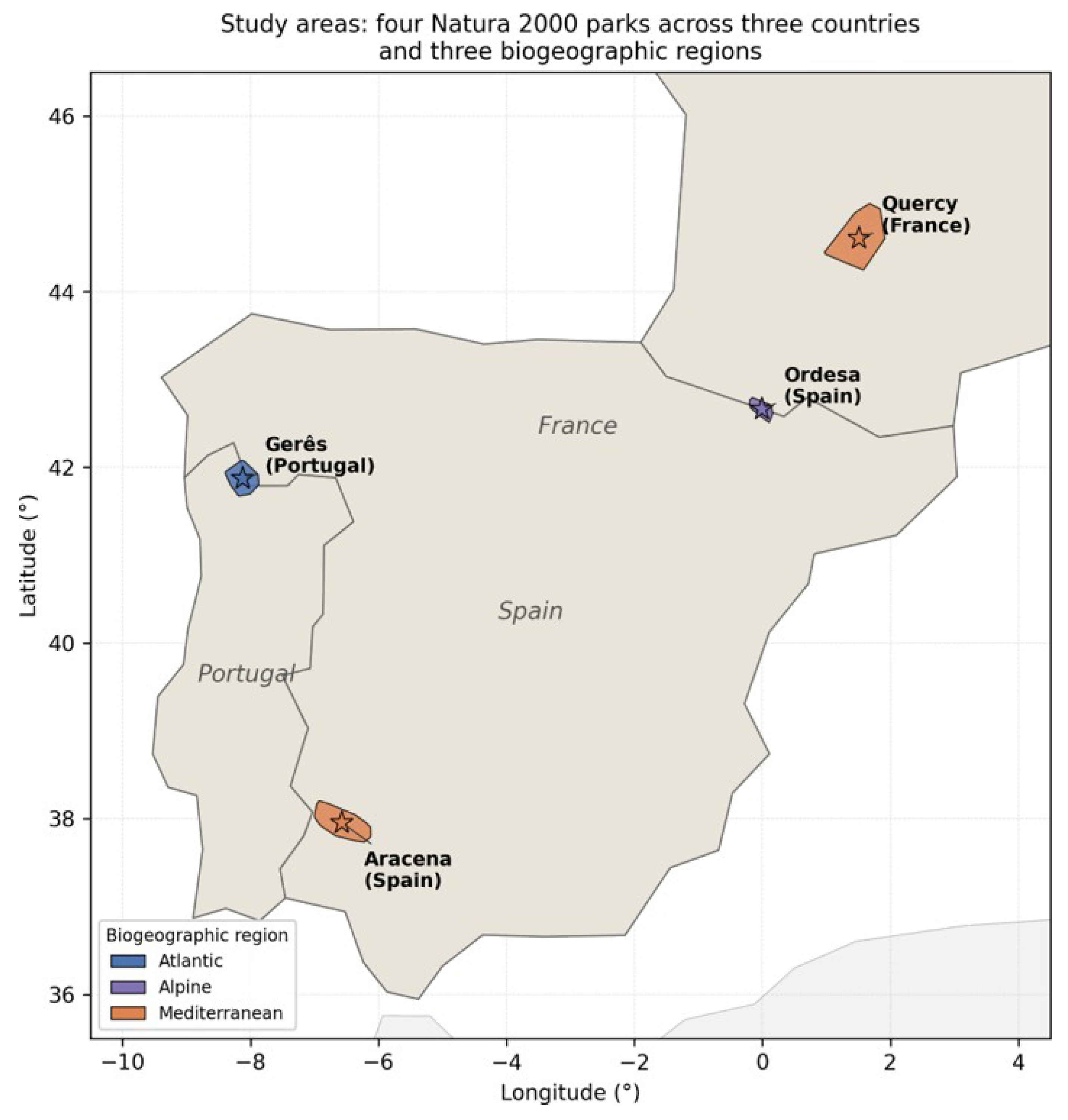
Figure 4.
Proposed architecture, shown in five stages: (a) three stochastically sampled Sentinel-2 timesteps (, bands) processed through a Conv3D input embedding; (b) the frozen Prithvi-EO-2.0 ViT-L backbone with LoRA adapters (, 6.3M trainable); (c) a Feature Pyramid Network (FPN) neck fusing multi-scale backbone features; (d) the UPerNet decoder with sinusoidal seasonal encoder and FiLM park-conditioning; (e) a final convolution head producing the binary habitat mask. Total parameters: 390.1M; trainable: 86.2M (22.1%). See Section 4 for full detail.
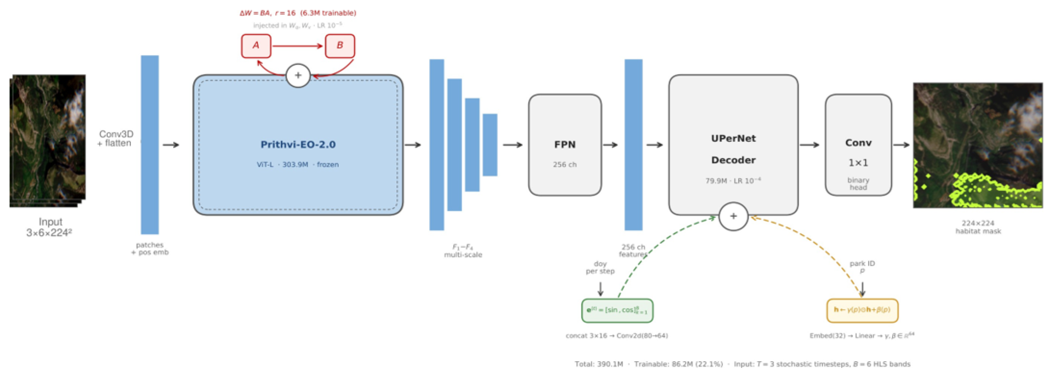
Figure 5.
LoRA injection into the frozen Prithvi-EO-2.0 backbone. LoRA modules () are applied to the combined qkv projection, the attention output projection (proj), and both feed-forward layers (fc1, fc2) of each transformer block, yielding 6.3 M trainable parameters ( of the 303.9 M backbone).
Figure 5.
LoRA injection into the frozen Prithvi-EO-2.0 backbone. LoRA modules () are applied to the combined qkv projection, the attention output projection (proj), and both feed-forward layers (fc1, fc2) of each transformer block, yielding 6.3 M trainable parameters ( of the 303.9 M backbone).
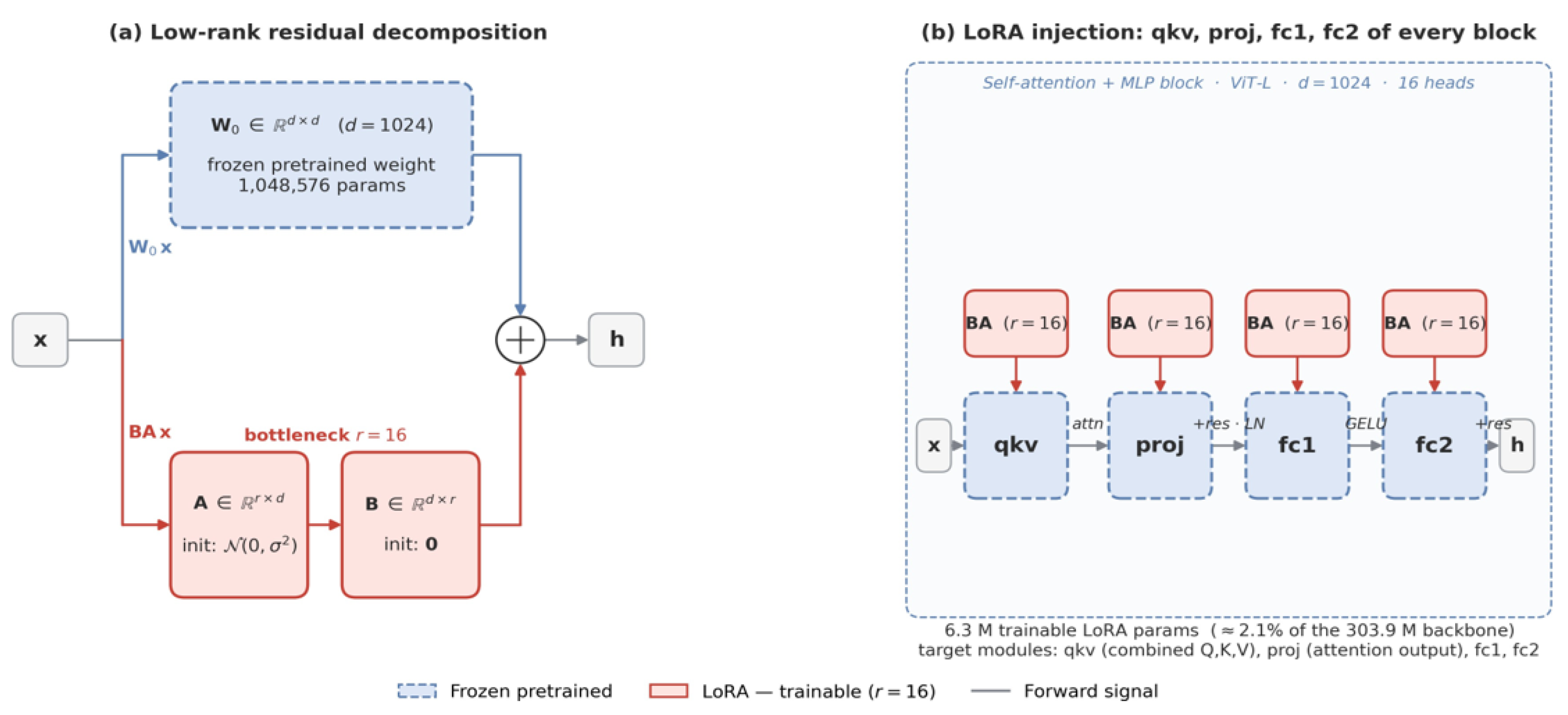
Figure 6.
Training strategy, illustrated on the 6210+6230 +Cat +Aragón Gerês fold. (a) Learning-rate schedule: 5-epoch linear warmup followed by cosine decay, with differential rates for the UPerNet decoder () and the LoRA modules (), common to every fold. (b) Composite loss trajectory (training and validation) for this fold: with label smoothing ; early stopping is disabled for this expansion-campaign fold (Table S4), so training runs the full 50 epochs and the best checkpoint (val mIoU 0.484, epoch 29, matching Table 4) is marked. (c) Per-habitat-class tile-sampler balancing weights (, binary positive rate shown); class imbalance spans two orders of magnitude (0.9%–63.1% positive pixels), motivating the weighted random sampler.
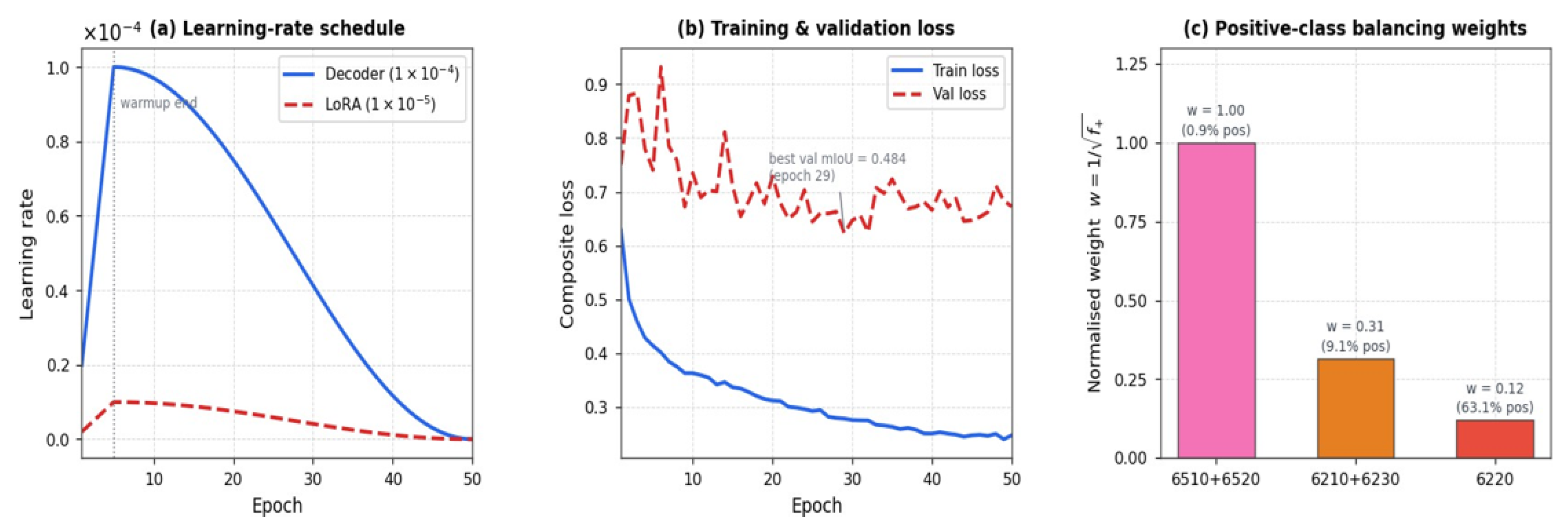
Figure 7.
Prediction gallery for the 6210+6230 +Cat +Aragón Ordesa expanded-training reference (mIoU 0.602, F1 0.519). Each row shows one of the 26 evaluation tiles used for this result, from five spatially distinct sub-regions of the park, labelled by tile centroid latitude/longitude; columns show the RGB Sentinel-2 composite (left), ground-truth mask (centre), and model prediction (right). Grey = non-habitat, yellow = calcareous grasslands (6210+6230), blue = no-data/ignore pixels.
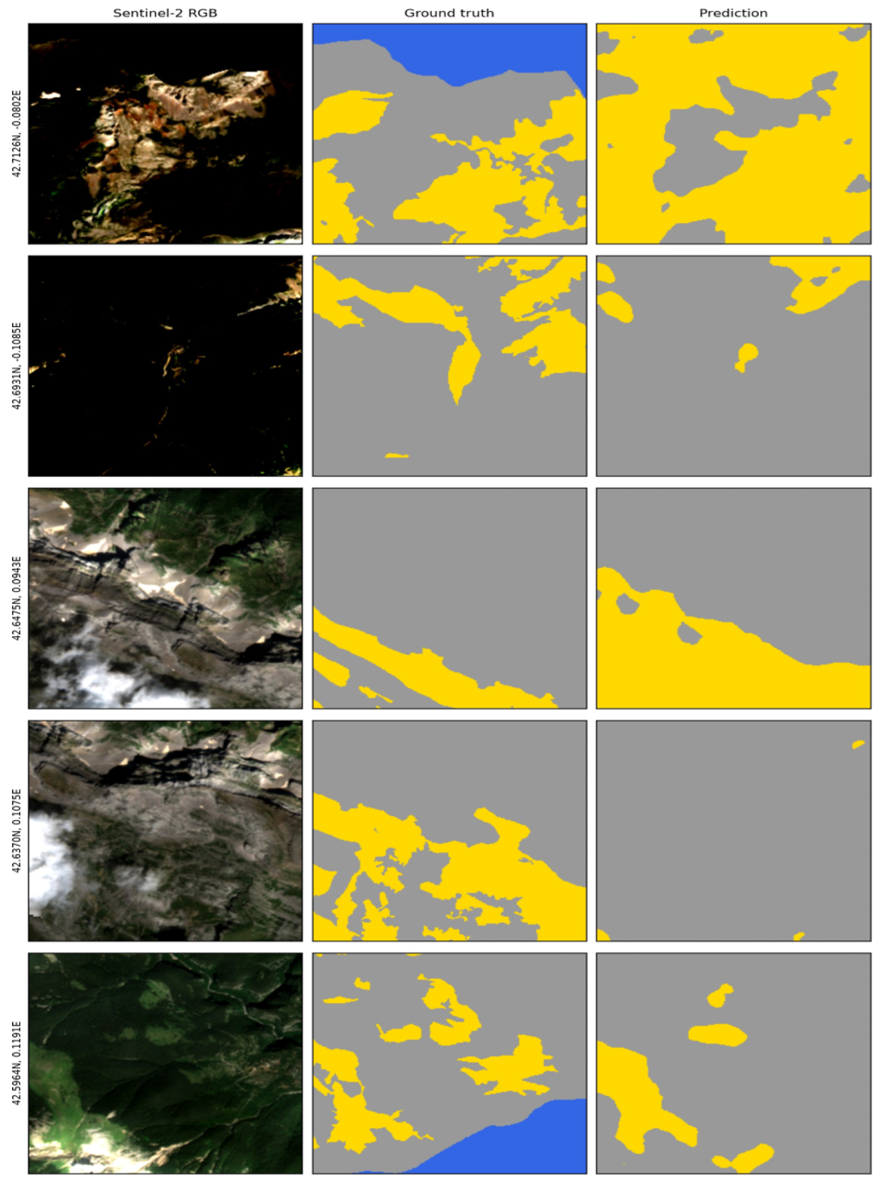
Figure 8.
6210+6230, val park: Gerês, +Cat +Aragón (LOPO fold)—real per-epoch validation curves for this fold’s actual training run (mIoU 0.484, F1 0.058, matching Table 4). Accuracy, mIoU, macro-F1, and Mean Dice are shown (macro-F1 and Mean Dice coincide exactly by construction for a binary task and overlap in the plot). Early stopping is disabled for this expansion-campaign fold (Table S4), so training runs the full 50-epoch budget; the best checkpoint (val mIoU 0.484, epoch 29, matching Table 4) is marked by the dashed line. Several earlier-vintage base-fold runs used patience-10 early stopping and stopped well short of 50 epochs instead (Section 6.4); the composite training loss for this same fold is shown separately in Figure 6.
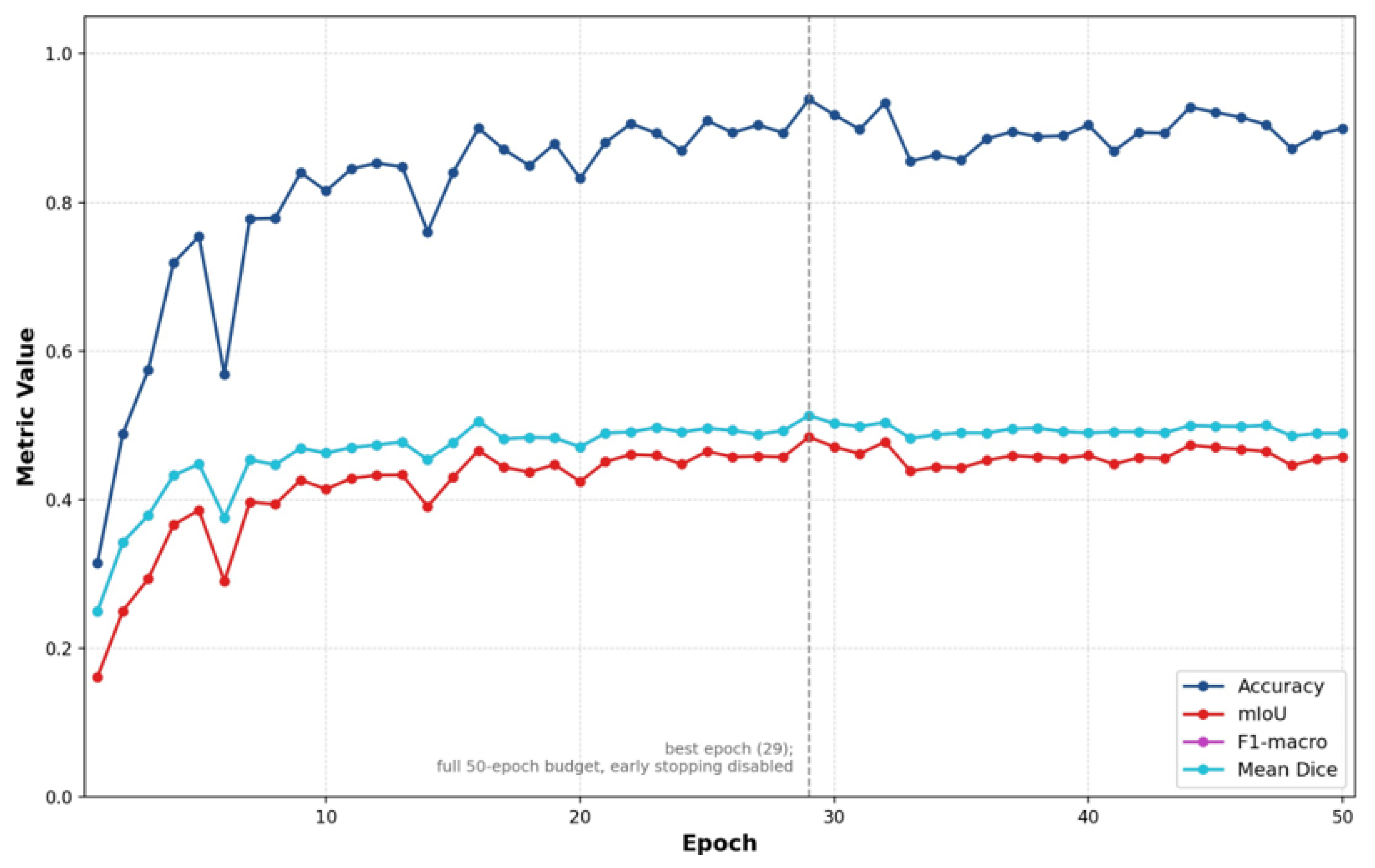
Table 1.
Primary N2K study areas. Shannon computed from the dominant habitat class raster. Label year is the year of the official N2K habitat inventory used as ground truth, not the Sentinel-2 acquisition year (the Sentinel-2 BAP archive uniformly covers 2018, 2024, and 2025 for all parks; see Section 3.2). Dominant-class polygon-area shares (different metric from the rasterised binary fractions in Table 3): Galicio-Portuguese oak woods 9230 at Gerês (43.5%), calcareous grasslands 6210 at Quercy (31.4%).
| Park | Country | Biogeographic region | Area (ha) | Types | Label year | |
|---|---|---|---|---|---|---|
| Ordesa | Spain | Alpine | 64,579 | 33 | 2.34 | 2018 |
| Aracena | Spain | Mediterranean | 145,952 | 22 | 2.44 | 2024 |
| Gerês | Portugal | Atlantic | 123,980 | 10 | 1.47 | 2017 |
| Quercy | France | Mediterranean | 35,110 | 23 | 2.58 | 2017 |
Table 2.
Relevant habitat grasslands evaluated in this paper and their occurrence across the primary study parks. All three are assessed under the Leave-One-Park-Out protocol, each being documented in at least two parks. Three further configurations (HCI 6140, 6170, 6310) are supported by the same data pipeline but are documented in only a single park each, so a LOPO protocol is not yet feasible for them; they fall outside the present scope (Section 6.4).
| Code | Habitat | Parks |
|---|---|---|
| 6210+6230 | Semi-natural dry + Nardus grasslands | Gerês, Ordesa, Quercy |
| 6510+6520 | Lowland + mountain hay meadows | Ordesa, Quercy, +Catalunya |
| 6220 | Thermo-Mediterranean grasslands | Aracena, Quercy |
Table 5.
Impact of Catalunya data expansion on 6510+6520 LOPO performance. Both binary mIoU and habitat-class F1 are reported per fold and as a per-fold mean. The F1 ratios reflect the order-of-magnitude lift (Ordesa F1 0.017 → 0.180) that is the underlying detection improvement; the smaller mIoU lift on the same fold is the background-class IoU artifact analysed in Section 5.1.
| Ordesa | Quercy | Mean | ||||
|---|---|---|---|---|---|---|
| Configuration | mIoU | mIoU | mIoU | |||
| Baseline (2 parks) | 0.459 | 0.017 | 0.475 | 0.034 | 0.467 | 0.026 |
| +Catalunya (3 tile regions) | 0.548 | 0.180 | 0.497 | 0.046 | 0.522 | 0.113 |
| (abs.) | +0.089 | +0.163 | +0.022 | +0.012 | +0.056 | +0.087 |
| (rel.) | +19.4% | ×10.6 | +4.7% | ×1.4 | +11.9% | ×4.4 |
Table 6.
Architecture comparison for the 6210+6230 +Cat +Aragón evaluation settings. Gerês and Quercy are directly comparable LOPO folds and are used to compute the architecture means. The Ordesa Prithvi result corresponds to the expanded-training reference of Section 5.3 (26 evaluation tiles), whereas the SwinV2 and U-Net Ordesa results use their respective full validation sets; Ordesa is therefore reported for reference only and excluded from the architecture means, and its cross-architecture differences should not be interpreted as a matched-split effect. Baselines differ from our model in backbone, decoder, pretraining, parameter count, and fine-tuning strategy (Table S2, Section 5.6). F1 95% CI: tile-level bootstrap (, percentile method).
| Val Park | Model | mIoU | F1 95% CI | Prec | Rec | |
|---|---|---|---|---|---|---|
| Gerês | Prithvi (ours) | 0.484 | 0.058 | [0.035, 0.085] | 0.037 | 0.142 |
| SwinV2-Tiny (3-stage, ImageNet) | 0.469 | 0.020 | [0.011, 0.031] | 0.012 | 0.057 | |
| U-Net (ResNet-50, random) | 0.425 | 0.051 | [0.037, 0.067] | 0.028 | 0.353 | |
| Ordesa | Prithvi (ours) | 0.602 | 0.519 | [0.396, 0.607] | 0.465 | 0.588 |
| SwinV2-Tiny (3-stage, ImageNet) | 0.532 | 0.540 | [0.508, 0.570] | 0.483 | 0.612 | |
| U-Net (ResNet-50, random) | 0.430 | 0.503 | [0.469, 0.534] | 0.371 | 0.783 | |
| Quercy | Prithvi (ours) | 0.446 | 0.152 | [0.114, 0.190] | 0.109 | 0.246 |
| SwinV2-Tiny (3-stage, ImageNet) | 0.464 | 0.144 | [0.098, 0.193] | 0.118 | 0.184 | |
| U-Net (ResNet-50, random) | 0.223 | 0.123 | [0.104, 0.144] | 0.068 | 0.616 | |
| Mean | Prithvi (ours) | 0.465 | 0.105 | — | 0.073 | 0.194 |
| SwinV2-Tiny (3-stage, ImageNet) | 0.467 | 0.082 | — | 0.065 | 0.121 | |
| U-Net (ResNet-50, random) | 0.324 | 0.087 | — | 0.048 | 0.485 |
Disclaimer/Publisher’s Note: The statements, opinions and data contained in all publications are solely those of the individual author(s) and contributor(s) and not of MDPI and/or the editor(s). MDPI and/or the editor(s) disclaim responsibility for any injury to people or property resulting from any ideas, methods, instructions or products referred to in the content. |
© 2026 by the authors. Licensee MDPI, Basel, Switzerland. This article is an open access article distributed under the terms and conditions of the Creative Commons Attribution (CC BY) license (http://creativecommons.org/licenses/by/4.0/).
Copyright: This open access article is published under a Creative Commons CC BY 4.0 license, which permit the free download, distribution, and reuse, provided that the author and preprint are cited in any reuse.