

Submitted:
29 September 2026
Posted:
30 September 2026
You are already at the latest version
Abstract
Hyperbolic geometry explains many structural features of real-world networks, yet existing hyperbolic generative network models with community organization such as the nonuniform popularity-similarity optimization (nPSO) are restricted to unipartite graphs. Here we introduce a bipartite extension of the nPSO model called nBPSO, motivated by the prevalence of community organization in real-world bipartite networks and the emerging evidence of hyperbolic hierarchical connectivity in trained sparse neural networks. nBPSO provides explicit control over link density, degree distribution, average clustering, and community organization. We engineer the model to generate consecutive and concatenated bipartite layers, enabling initialization of dynamic sparse training multilayer perceptron neural networks with tunable hyperbolic organization for each layer. We find that task-agnostic (unaligned with the task) hyperbolic random network initialization degrades the performance of sparse neural networks compared with uniform random initialization. This degradation arises because the hyperbolic random initialization imposes an arbitrary hierarchical prior into the sparse topology. Dynamic sparse training may then need to optimize the weights and reorganize this arbitrary task-agnostic hierarchy into a task-driven one. By contrast, a uniform random initialization imposes at start less structural bias and may therefore be easier to reconfigure during training toward the hierarchical topology suited to the task. This work motivates the need for data-informed hyperbolic initialization methods which generate sparse topologies with a hierarchical prior closer to the task, facilitating the further learning of a task-oriented hierarchical organization during dynamic sparse training. In addition, nBPSO represents the first hyperbolic bipartite network generative model that allows the mesoscale community structure to be explicitly controlled through model parameters, making it a useful tool for broader complex systems applications where community organization is central to accurate and interpretable modeling.
Keywords:
sparse neural networks
; sparse training
; sparse initialization
; network geometry
; geometry-informed learning
; network science
; complex systems
I. Introduction
Hyperbolic space has been shown to effectively explain underlying structural features of complex, real-world networks [1,2,3,4,5,6,7]. In this context, the popularity-similarity optimization (PSO) [8] model simulates how random geometric graphs grow within a hyperbolic space. The PSO model generates realistic networks with high clustering, small-worldness, scale-freeness, and rich-clubness. In the PSO model, radial coordinates represent the popularity of a node on the hyperbolic disk (the higher the node degree, the closer to the center of the disk), while the angular coordinates represent node similarity (nodes sharing a similar connectivity pattern are angularly closer). The nonuniform popularity-similarity optimization (nPSO) [9] model extends the PSO model by introducing heterogeneous angular node arrangement, providing the ability to explicitly create and set the number and size of communities within the network.
Because of its ability to generate realistic topologies with a known ground-truth geometry and community organization, the nPSO model has been frequently used to benchmark community detection [10,11], greedy routing [12], and link-prediction [13,14,15] algorithms. It has also been used to evaluate methods that separate mesoscale patterns in data [16], as well as those assessing geometrical congruence [12], a measure that quantifies the extent to which the topology of a network follows an underlying geometry. Furthermore, it has been employed to validate latent-geometrical approximators, such as those used for network dismantling [17] and network embedding [18] and other embedding methods [19]. However, the nPSO generates unipartite networks, whereas bipartite systems have two node types with links only between the types [20]. Among the first studies on bipartite geometric graphs we recall the AB random geometric graph (AB RGG) model [21], which uses Euclidean space where two independent Poisson processes generate points for each set and connections are established when the distance between points from opposite sets falls below a threshold. Separately, the S1 [22] and H2 ADDIN ZOTERO_TEMP [3] models demonstrated that unipartite networks can be effectively modeled in a latent geometry, where the angular coordinate encodes similarity. This model was subsequently extended to the bipartite case, first as the S1 × S1 model (using Euclidean space) to study metabolic networks [23], and later in an equivalent hyperbolic formulation as the H2 × H2 framework to analyze the latent geometry of bipartite systems [24]. This notation emphasizes the two node types sharing a common latent space. Related work developed an asymmetric PSO method to embed directed networks (modeled as bipartite structures) into hyperbolic space [25], and other work coupled node networks to node–feature bipartite graphs, with implications for graph neural networks [26]. More recently, the Sd/Hd+1 model extended the original model to embed bipartite networks into multidimensional hyperbolic spaces [27]. Also the PSO framework was recently extended to the bipartite case [28]. However, all these hyperbolic bipartite models focus on generating artificial networks without tunable topological properties that can explicitly control the community organization. To address this gap, here we introduce a bipartite extension of the nPSO model called nonuniform bipartite PSO (nBPSO), which provides explicit control over link density, degree distribution, average clustering, and community organization. With respect to the previous nPSO study, we now provide an empirical analysis of the clustering modeling limits, and we achieve a practical runtime speedup for the edge-case setting of temperature T = 1. Additionally, we introduce a spread factor to control community compactness, and a rewiring mechanism that allows us to modify the hierarchical organization on each bipartite layer.
It has been shown that real bipartite networks also live in a latent geometrical space [23,24], and such bipartite networks may also exhibit a hyperbolic structure. Bipartite representations are useful for user-item recommendation systems [29], metabolic networks [30], ecological plant-pollinator mutualisms [31], and collaboration networks [32]. Therefore, introducing the nBPSO can be practically useful to model the community organization in real-world bipartite networks, but also to model the emerging evidence of hyperbolic bipartite hierarchical connectivity in trained sparse multilayer perceptron (MLP) neural networks [33]. This second motivation is the focus of the present study, and it arises from the growing intersection between hyperbolic network geometry and artificial intelligence, an area that has recently attracted substantial attention. It has been shown that hyperbolic hierarchy, the hierarchical organization revealed when a network is embedded in a hyperbolic space, emerges in dynamic sparse training of neural networks [33]. Specifically, MLP neural networks, whose bipartite layers are sparsely initialized uniformly at random, naturally evolve during training to learn a final sparse topology that displays task-oriented hyperbolic hierarchical organization [33]. Crucially, because the architectures of many feed-forward deep neural networks are fundamentally bipartite (e.g., between consecutive layers), a bipartite adaptation of the nPSO model is uniquely suited for initializing the next generation of these hyperbolic neural networks. Therefore, in this study we engineer the nBPSO to generate consecutive and concatenated bipartite layers, enabling initialization of dynamic sparse training MLP neural networks with tunable hyperbolic organization for each layer. Then, we show that the nBPSO can be used as a model to analyze the impact of hyperbolic network geometry, hierarchy, and communities in dynamic sparse training of neural networks.
Finally, we clarify that this study is the first to discuss the impact of hyperbolic sparse network topology on neural network training, meaning that the sparse network topology is generated in a latent hyperbolic space. This should not be confused with previous literature that primarily focused on investigating fully connected hyperbolic neural networks [34,35], where the data [36] and graph [37,38] embeddings, as well as the mathematical operations [39] on the link weights, are performed natively within the hyperbolic space, as this geometry enables these models to inherently capture the hierarchical and complex relational structures of higher-dimensional data.
II. Nonuniform Bipartite PSO (nBPSO)
The nonuniform bipartite popularity-similarity optimization (nBPSO) model is a generative network model that extends the nPSO model to construct realistic bipartite networks in hyperbolic space. It optimizes the trade-off between node popularity, represented by the radial coordinate, and node similarity, represented by the angular distance. It employs a nonuniform angular distribution to explicitly generate distinct community structures while resembling the density, scale-freeness, clustering, and small-world properties of real networks. To achieve a bipartite topology, the model grows two disjoint sets of nodes, set A and set B, interleaving their generation and restricting edge formation strictly between the two sets.
- A
- Model Parameters
The nBPSO model is defined by the following input parameters:
NA and NB: The total number of nodes in set A and set B, respectively, yielding a total network size of N = NA + NB.
mAB or d (network density): The parameter mAB controls the number of edges formed when a new node is introduced; this value is approximately equal to half the average node degree. As an extension to the original models, we allow d as a direct input parameter, to explicitly set the network density. When density is provided, the model automatically approximates the necessary mAB :
Supplementary Figure S1 shows that the target density is largely achieved as expected. However, at higher densities the realized density is slightly lower than the target. This occurs because early-generated nodes cannot yet reach the target mAB when the network is still small, and this mismatch becomes more pronounced as density increases.
T: The network temperature, strictly bounded to T ∈ [0,1], which is inversely related to the level of clustering. While the original PSO and nPSO models theoretically permit T > 1, clustering decreases almost linearly for T ∈ [0,1] and becomes practically unrelated to geometry (uniformly random) for T ≥ 1, making the bounded range sufficient. Indeed, we see in Supplementary Figure S2(a), in the original nPSO model, that when T = 1, the connection probabilities are all very small and practically the same. Hence, a small improvement we make from the original model is that we bypass all hyperbolic distance calculations when T = 1 and enforce uniform at random sampling of connections for a new node (see Figure 1(a.1)). As detailed in Appendix A, this reduces computational complexity from O(N2 + ElogN) to O(E) when T = 1, while the resulting model remains equivalent. Supplementary Figure S2(b) shows that this speedup becomes apparent for network sizes of N = 50,000 and above. When T = 0 (Figure 1(b.1)), a new node strictly connects to only the geometrically closest nodes (rigid connection scheme); when 0 < T < 1, a new node connects progressively more randomly with respect to the underlying geometry (soft connection scheme); when T = 1, it connects uniformly at random regardless of the geometry.
γ: The target exponent of the power-law degree distribution (γ ≥ 2) which conditions the popularity fading parameter, During the network growth process, β governs how quickly nodes move from the center to the periphery, according to the radial coordinate formula (Eq. (2) and Eq. (3) provided in section II.B.c). β = 1 (γ = 2, Figure 1(b.1)) corresponds to no radial popularity fading; this means that the older nodes with higher degree lie at the center of the embedding and since the network has a higher node degree heterogeneity then it has also a stronger hierarchical arrangement. Higher γ means the degree distribution is less power-law, thus the network is less hierarchical. Indeed, progressively smaller β relates to higher γ that in turn means the degree distribution becomes increasingly homogeneous and the hierarchical organization of the network fades away, causing older nodes (which have higher degree) to drift outward more strongly, taking radial coordinates closer to the circumference (for instance, see , which corresponds to γ = 3, Figure 1(c)).
The nBPSO introduces an innovation that is an optional rewiring (random, regular, or tight) step. Both random and regular preserve the degree of nodes in set A while destroying the original power law degree distribution of set B. Random (Figure 1(b.2), left) rewiring reassigns all edges uniformly at random for set B, yielding a binomial-like distribution centered at the average degree. Regular (Figure 1(b.2), right) rewiring forces every node in set B to have the same degree, resulting in a regular graph with constant degree across all set B nodes. These rewiring mechanisms are particularly useful for testing different hierarchical arrangements (topological dependence) on the two layers of a neural network. In addition to random and regular rewiring, we introduce a tight rewiring method. Tight rewiring preserves the exact degree of every node in both sets and operates by swapping only inter-community edges (edges connecting nodes from different communities) to turn them into intra-community edges. It does so by exchanging the opposite-set endpoints of two inter-community edges. This process reduces community mixing. Community mixing quantifies the extent to which edges connect nodes from different communities rather than within the same community. Unlike random or regular rewiring, tight rewiring retains the original power-law degree distribution of both sets because it preserves individual node degrees. We see that tight rewiring successfully reduces community mixing in Figure 2.
: The parameter ζ scales the hyperbolic space, where K is the curvature of the hyperbolic plane. As in the nPSO model, we always set K = −1 (negative curvature), because modifying ζ merely rescales the radial coordinates without affecting the topological properties of the network [8].
We can model communities using a generalized mixture of any type of distributions, as shown in the original nPSO study [9]. However, without loss of generality, in this study we focus on the most widely used Gaussian mixture distribution, parameterized by:
- -
- C: The number of components, each one representative of a community. For C ≥ 1, angular coordinates are sampled from a mixture containing C components. We use C = 0 as a special convention denoting uniform angular sampling with no prescribed community structure (equivalent to the PSO model).
- -
- μ1…C ∈ [0, 2π): The means of the components, representing community centers in the angular space
- -
- σ1…C > 0: The standard deviations, determining community angular spread; a lower deviation results in isolated communities, while a higher deviation leads to overlapping boundaries.
- -
- ρ1…C > 0: The mixing proportions, defining the relative sizes of the communities.
As in the nPSO model, we fix these variables by default to a straightforward setting that generates equally sized and reasonably isolated communities. We introduce the ability to explicitly set what we term the spread factor s > 0 (s = 6 was used in the nPSO model) to control community compactness: higher s yields tighter, more isolated communities. Specifically, we enforce:
, for i = 1 … C: Arranging the means equidistantly over the angular space.
: Setting the standard deviation to a fraction 1/s of the distance between two adjacent means.
: Fixing equal mixing proportions.
We show in Supplementary Figure S3 the effect of the spread factor on the community mixing. We see that in the no-rewiring case, increasing the spread factor reduces community mixing.
- B Generative Algorithm
The nBPSO network is generated in the hyperbolic disk as follows:
- Angular coordinate initialization
Initially, the network is empty. Before the growth process begins, all N nodes are assigned an angular coordinate θ ∈ [0, 2π). To confer an explicit community structure, these angles are sampled nonuniformly from the fixed Gaussian mixture distribution defined by C. Nodes are assigned to the community whose mean μC minimizes the angular distance to their sampled θ.
- b. Interleaved node appearance
The network grows over global time steps t = 1,2,…,N = NA + NB. To balance the bipartite structure, nodes from set A and set B are introduced in an interleaved sequence. Specifically, for every single node introduced to set A, a sequence of nodes is introduced to set B. When n is not an integer, the model interleaves nodes by adding ⌊n⌋ or ⌈n⌉ B-nodes per A-node, ensuring that the total numbers match NA and NB.
In addition to the global sequence time t, we define independent set-specific logical times tA and tB, which count the appearance order of nodes within each set. These set-specific times are used for radial evolution so that popularity fading reflects the actual number of nodes added to the corresponding set. This is particularly important when (NA ≠ NB): using the global time would cause the radial coordinates of nodes in the smaller set to evolve according to growth occurring partly in the opposite set, rather than according to the number of new nodes introduced within their own set. Using tA and tB therefore preserves the intended popularity-fading dynamics independently within each node set.
- c. Radial coordinate assignment and popularity fading
When a new node i appears at global time t, it is placed at the edge of the disk with an initial radial coordinate based on its set-specific logical time:
where tset,i is the logical time of node i within its own set. Using a set-specific time preserves the original interpretation of radial coordinates as relative node popularity, applied independently to the two bipartite node sets. Using global time instead would cause arrivals in the opposite set to artificially advance the radial evolution of a set even though no new node had appeared within that set.
Simultaneously, all previously existing nodes j in the same set experience popularity fading, drifting outward from the center. Their radial coordinates are updated according to:
where β regulates the fading speed.
- d. Bipartite edge formation
When a new node i belonging to set B appears, it attempts to connect to mAB previously existing nodes in set A. Conversely, when a set A node appears, it connects to previously existing nodes in set B. For 0 < T < 1, the connection weight used for sampling an edge between node i and an existing candidate node j in the opposite set is:
For 0 < β < 1, Ri is the current radius of the hyperbolic disk governing the target set, defined as:
For β = 1, Eq. (5) is evaluated using the limiting form since .
Here, dij is the hyperbolic distance between the two nodes, calculated as:
where ∆θij = π − |π − |θi − θj|| is the angular distance between them.
dij = arccosh(cosh ricoshrj − sinh ri sinhrj cos∆θij)
If T = 0, the new node connects deterministically to the mAB hyperbolically closest nodes in the opposite set. For 0 < T < 1, the connections are sampled probabilistically based on p(i,j). As explained previously, when T = 1, the connections are chosen uniformly at random.
III. nBPSO Model Properties
- A
- Community Mixing
Figure 2 compares community mixing across rewiring methods. The original non-rewired network already exhibits strong community structure due to the nonuniform angular sampling. random and regular rewiring both increase community mixing; edges become more evenly spread across communities because they ignore community labels during edge reassignment. tight rewiring, however, explicitly swaps inter-community edges to create intra-community ones, thereby reducing community mixing and producing stronger, more isolated communities than the original network.
- B Scale-Freeness
The rewiring mechanism enables custom degree distribution profiles across node sets. This is important because real-world bipartite networks frequently exhibit asymmetric degree distributions; for example, one node set follows a power law distribution while the other set is more homogeneous [40]. In addition, hyperbolic hierarchy associated to scale-free connectivity has been shown to be functionally important in sparse neural networks (of which the layers are bipartite networks). Specifically, Cannistraci-Hebb Training (CHT) - by Zhang et al. (2024) [33,41] – is a dynamic sparse training method that rewires connectivity during learning by removing a certain fraction of links with lower absolute weights and replacing them with epitopological learning implemented via CH link prediction [42]. CHT was shown to produce sparse trained neural networks that are scale-free and develop a form of meta-depth (hierarchy of nodes with different degree inside each layer).
We quantitatively assess the scale-free nature of the node degree distributions of different networks using the tail-index estimator proposed by Voitalov et al. [43], ξmin (the minimum ξ estimator), which accounts for finite-size sampling noise (Supplementary Figure S4). A network is considered: not power-law if ξmin ≤ 0; hardly power-law if 0 < ξmin ≤ 0.25 and power-law if ξmin > 0.25. For set A (which is never rewired), the power-law behavior depends on network size and density. For smaller networks, the distribution is typically in the weak regime, whereas larger networks exhibit a stronger power law. However, as density increases, the power-law becomes progressively weaker. This occurs because higher density makes it harder for any single node to have a much higher degree than others; the degree distribution becomes more homogeneous and less power-law. A higher temperature also yields a weaker power-law distribution, as the connections become more random and deviate more from the underlying (hyperbolic and hierarchical) geometry. For set B, without rewiring, its degree distribution follows the same power-law pattern as set A. Tight rewiring does not change the degree distribution as the degree sequence is perfectly preserved. Under random or regular rewiring, the power-law distribution is effectively destroyed; random rewiring yields a binomial distribution, while regular rewiring forces every node in set B to have exactly the same degree.
- C Clustering
Another key innovation of our nBPSO model with respect to the previous unipartite model nPSO is the ability to explicitly set a target clustering, given the constraints set by the original nPSO model. If one chooses a target clustering instead of a temperature T, the model will use an automated bisection search to find the temperature that yields a clustering as close as possible to the desired target, which may be limited by the growth mechanism of the nPSO model. The bisection search begins by defining an initial search interval, bounded between maximum clustering (T = 0) and minimum clustering (T = 1). In each iteration, the midpoint temperature of the current interval is calculated (T = 0.5 for the first iteration), and a network is generated at this exact temperature, and its bipartite clustering coefficient is computed. The search bounds are then updated based on how this measured clustering compares to the target. Because of the inverse relationship between temperature and clustering, if the measured clustering is higher than the target, the algorithm infers that a higher temperature is needed, and the lower bound is shifted up to the current midpoint. Conversely, if the measured clustering is lower than the target, a lower temperature is required, and the upper bound is shifted down to the midpoint. This iterative halving of the search space continues until the optimal temperature is found. An early stopping mechanism is implemented, terminating the search if the measured clustering matches the target when both are rounded to two decimal places. If a match is not achieved, the process halts after a maximum number of iterations (set by default to 20), returning the temperature that best approximates the target clustering.
We use the Robins–Alexander clustering coefficient [44] for bipartite networks, defined as:
where C4 is the total number of four-cycles in the network and L3 is the total number of three paths in the network. A four-cycle (square) is a closed loop of four distinct nodes alternating between sets A and B, uA − uB − vA − vB − uA, with alternating node sets. A path of length three is an open chain of three edges connecting four distinct nodes, also alternating sets, uA − uB − vA − vB. The factor 4 in the numerator compensates for the fact that each four-cycle contains exactly four distinct 3-paths (one for each edge that can be removed), whereas the cycle itself is counted only once in C4. The factor 4 ensures that 4∙C4 counts the number of 3-paths that are closed into 4-cycles. Dividing by L3 thus yields the fraction of all 3-paths that are closed, analogous to the standard clustering coefficient for unipartite graphs.
We find in Figure 3 that the achievable bounds of the Robins–Alexander clustering coefficient, with no rewiring, range from 0.02 to 0.61. These bounds are inherent constraints imposed by the original nPSO model mechanism. Supplementary Figure S5 shows the clustering coefficient bounds for all rewiring cases.
Additional analysis on the characteristic path length (CPL) and assortativity is discussed in Appendix B and in Supplementary Figure S6 and Figure S7, respectively.
IV. Hyperbolic Network for Sparse Neural Network Initialization
- A
- Layered nBPSO
The nBPSO model described thus far generates a single bipartite structure between two node sets (e.g., input layer–hidden layer or between two hidden layers). To initialize an MLP with multiple nBPSO generated sparse network layers (Figure 1 (d)), for instance, an input layer (A), three hidden layers (B, C, and D), we need a layered nBPSO that simultaneously builds all consecutive bipartite networks, XAB, XBC, and XCD, in a coherent manner. This enables us to initialize an inherently hyperbolic sparse neural network.
- Growth procedure
The layered extension follows the same growth process as the nBPSO, but with multiple layers interleaved. All nodes from all layers share the same hyperbolic disk (Eq. (2)), draw angular coordinates from the same distribution (Gaussian mixture for communities, uniform for no communities), and follow the same radial fading rule (Eq. (3)). The birth order interleaves layers in a consecutive fashion (one from A, then B, then C, then D, repeating). This allows a new node to connect to previously existing nodes in both the preceding and following layers. For each adjacent pair of layers, the connection weight used for sampling is given by Eq. (4).
- 2.
- Rewiring per layer pair
The optional rewiring step is applied independently to each bipartite adjacency matrix (XAB, XBC, and XCD). We can choose which set the rewiring modifies. For example, if we choose the right-hand node set to be modified (B in A–B, C in B–C, D in C–D), it is the in-degrees of layers B, C, and D that are rewired and for which the power-law node degree distribution is modified (can be transformed into a binomial distribution or regular distribution, see section III.B), while the out-degrees (to the next layer) remain power-law, because those out-degree distributions originate from separate matrices where the layer appears on the left (A in A-B, B in B–C, C in C–D) and are never rewired.
- A.
- nBPSO as a model for sparse neural network initialization
In this study, we investigate and design the nBPSO model because we need a modeling tool that allows us to address a key open question in dynamic sparse training (DST) of neural networks such as MLPs: “Is a task-agnostic (arbitrary) hyperbolic hierarchical random network initialization able to trigger performance gains larger than a uniform random network initialization? Or should the hyperbolic hierarchical random network organization emerge as a task-driven hierarchy learned during training by epitopological learning (the process of learning a topology by topologically predicting the network's connections over the course of training) [33]?” The layered nBPSO allows us to answer this question by initializing sparse neural networks with controlled hyperbolic hierarchical architectures and evaluating their respective performance.
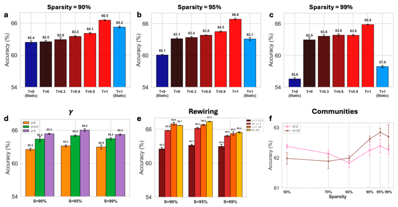
Figure 4 shows results on the CIFAR-10 image recognition task using networks trained with the current state-of-the-art DST method, Cannistraci-Hebb training soft rule (CHTs). In Figure 4(a, b, c), a strictly hyperbolic hierarchical initialization (temperature T = 0, meaning the network strictly follows the hyperbolic geometry) performs worse than one where connections are set uniformly at random (T = 1, Erdős–Rényi-like). This trend holds for both CHTs and “Static” (without topology evolution), different sparsity levels, and with or without communities (Supplementary Figure S8), where performance improves as temperature increases (i.e., as coupling between topology and hyperbolic geometry decreases).
In other words, imposing an arbitrary task-agnostic hyperbolic hierarchical topology at initialization reduces the network's ability to learn a task-driven hyperbolic hierarchical geometry. Because the training process may be constrained by an initial hyperbolic organization whose hierarchy is not aligned with the task, and the model may fail to benefit from this hyperbolic hierarchical structure. Full experimental setup is detailed in Appendix C.
We further examined the impact of the power-law exponent γ, which controls the level of hierarchy (Figure 4(d)). A higher γ, implying a weaker power-law and thus less hierarchy, improves performance. The improvement is notably larger for CHTs than for Static (Supplementary Figure S9).
We next analyzed the effect of breaking the power-law degree distribution, and thus the hierarchy, of layers via random rewiring (Figure 4(e)). When random rewiring is applied, the network becomes effectively Erdős–Rényi-like (ER). Random rewiring is applied to the left-hand side layer (named “ER − γ = 2”), right-hand side layer (“γ = 2 − ER”), or both (ER − ER). For CHTs, rewiring the left-hand side, right-hand side, or both layers causes a substantial jump in performance, with rewiring both layers typically achieving the best results. Again, we show our results hold for different settings (Supplementary Figure S10).
Overall, the fact that a less pronounced arbitrary hierarchy at initialization (either by increasing γ or by rewiring the sets) improves performance in CHTs aligns with our previous observations: a data-agnostic hyperbolic network hierarchy at initialization is especially detrimental to CHTs because it hinders the model’s learning of a task-driven hierarchy.
Finally, we find that at lower levels of sparsity (50% to 70%), having fewer communities in the network improves the performance of CHTs (Figure 4(f)). However, at sparse and ultra-sparse levels (80% to 99%) in the network, a larger number of communities (10 rather than 2) starts to improve the performance of the model.
Our nBPSO therefore serves as a powerful reference model for investigating the impact of hyperbolic network geometry initialization on dynamic sparse training of neural networks such as MLP via epitopological learning.
V. Conclusions
In this work, we introduced nBPSO, a bipartite extension of the nPSO model that generates realistic hyperbolic networks with tailored community organization between two disjoint node sets. We enhanced the model with explicit control over density and clustering, including a bisection search to achieve a target clustering coefficient, and we demonstrated a practical runtime speedup for the edge-case temperature T = 1 by bypassing hyperbolic distance calculations. We also introduced a spread factor to tune community compactness and, importantly, a rewiring mechanism that can modify the degree distribution on one layer; either strengthening the scale-free structure or deliberately destroying it.
By extending this model to consecutive layers, we initialized multi-layer perceptrons (MLP) where we can explicitly control the density, degree distribution, average clustering, and community organization with tunable hierarchy, and community structures. Operating as a reference generative model, this layered nBPSO allowed us to systematically evaluate the role of hierarchy generated by hyperbolic geometry in sparse neural networks. Crucially, we demonstrated that imposing an arbitrary task-agnostic hyperbolic and hierarchical sparse network at initialization harms performance especially in the case of dynamic sparse training via CHTs. This is because this arbitrary hyperbolic hierarchy induces a structural bias that hinders the model’s learning of a task-driven hierarchy. Therefore, in our second study [45], we investigate how to leverage data-informed hyperbolic initializations to improve sparse neural network performance.
Supplementary Materials
The following supporting information can be downloaded at the website of this paper posted on Preprints.org.
Author Contributions
ZL and CVC conceived the initial nBPSO model and ZL implemented the first code. JC improved and optimized the code. TA and CVC expanded the nBPSO model and TA implemented the changes in the code. TA and CVC planned the article, and TA and WG ran the experiments and TA made the figures. TA wrote the draft of the article. CVC and JC corrected and improved it to arrive at the final draft. CVC supervised the study.
Data Availability Statement
The code will be available upon acceptance of the paper, where all the data generated for this article can be reproduced. Both MATLAB and Python versions will be available for the original unipartite PSO and nPSO models as well as the proposed nBPSO and layered nBPSO. We used the original CHTs code (github.com/biomedical-cybernetics/Cannistraci-Hebb-training) for sparse neural network training.
Acknowledgments
This work was supported by: The National Natural Science Foundation of China grant number W2531064 to C.V.C. The Zhou Yahui Chair Professorship award of Tsinghua University to C.V.C. The National High-Level Talent Program of the Ministry of Science and Technology of China grant number 20241710001 to C.V.C.
Appendix A. Computational Complexity
The nBPSO generates nodes sequentially, interleaving sets A and B. At each iteration i (total N = NA + NB nodes), the new node connects to mAB existing nodes in the opposite set. The computational complexity closely follows that of the original nPSO:
When mAB≈N (degenerate case): the new node connects to all previous opposite-set nodes. At iteration i there are at most i − 1 such nodes, requiring O(i) operations. Summing over i = 1 to N:
When mAB≪N (realistic case), a new node will connect to mAB number of existing opposite-set nodes:
- -
- When T = 0 (deterministic): For each iteration i, compute hyperbolic distances to all existing opposite nodes (O(i) operations). Then find the mAB smallest distances. Using a min-heap, building the heap costs O(i), and retrieving the mAB smallest distances costs O(mAB log i). Total per iteration: O(i + mABlogi). Summing:
where E≈mABN is the total number of edges.
- -
- 0 < T < 1 (probabilistic): Using non-uniform sampling, for each iteration i, compute hyperbolic distances to all existing opposite nodes (O(i) operations). Then perform a weighted sampling without replacement for mAB links (costing O(mAB log i)). Total per iteration is O(i + mABlogi) and summing gives us the final computational complexity of O(N2 + ElogN), as in Eq. (9).
- -
- T = 1 (fully random): no distances or probabilities are computed; we simply pick mAB random opposite nodes. This costs O(mAB) per iteration, giving:
Regarding the rewiring step, if no degree information is precomputed, both rewiring methods first require computing the degree of set A nodes, which in the worst case is O(N2), or O(E) in a sparse graph. After obtaining degrees, random rewiring reassigns each edge by choosing random opposite-set nodes, costing O(E). Regular rewiring additionally computes a degree budget for set B nodes and then reassigns each edge once, also costing O(E).
For tight rewiring, we first identify all inter-community edges in O(E). The algorithm then greedily swaps pairs of such edges to convert them into intra-community connections, while preserving the degree of every node. After each swap, the set of current inter-edges is updated in O(1) using a dynamic set structure. A heuristic limit of 2 × ∣inter_edges∣ is placed on the number of successful swaps. In the worst case, scanning for swappable pairs may lead to O(E2) operations.
In summary, the nBPSO inherits the asymptotic computational complexity of the original nPSO in most cases. At T = 1, we even bypass distance and sampling-weight calculations entirely, yielding O(E) operations instead of the original’s O(N2 + ElogN).
In addition, the bipartite case considers, at each iteration, only opposite-set nodes rather than all previous nodes. The fraction of opposite-set nodes varies with the relative sizes of the two sets, but it is always a constant factor (≤ 1). This reduces the constant factor without changing the asymptotic complexity. Consequently, the bipartite extension incurs no additional asymptotic overhead and offers a practical runtime speedup.
Appendix B. Topological Measures
Below we report additional topological properties of the networks generated by the nBPSO model under different parameter settings.
- Characteristic path length (CPL)
The characteristic path length (CPL) is the average of the shortest path lengths between all pairs of vertices in the network [46]. For bipartite graphs, paths alternate between the two sets.
In Supplementary Figure S6, we see that tight rewiring generally has a small effect on CPL. The same is true for random rewiring because the resulting binomial degree distribution is still associated with short CPL, like an Erdős–Rényi random graph. Finally, regular rewiring increases CPL, most visibly in small sparse networks. The power-law distribution gives shorter CPL due to hubs [30]; converting set B to a constant degree profile removes those hubs, which increases the CPL.
In general, as density increases, CPL decreases because additional edges create more bridges across the network. Higher temperature, which makes the network less clustered, also leads to a slightly higher CPL.
- 2.
- Assortativity
Cross-set assortativity measures the Pearson correlation coefficient between the degrees of nodes connected by an edge, where the two endpoints belong to different sets (A and B). It quantifies the tendency of high-degree nodes in one set to connect to high-degree (assortative) or low-degree (disassortative) nodes in the opposite set [47].
As seen in Supplementary Figure S7, in the standard (no rewiring) case, networks are weakly disassortative (slightly negative coefficient). This is expected for scale-free bipartite networks, where hubs in one set tend to connect to many low-degree nodes in the opposite set. This is an important property of scale-free networks: the presence of hierarchy is incompatible with an assortative structure.
As temperature T increases (more random connections), the assortativity moves closer to neutral (near zero). Rewiring (tight, random or regular) also makes the network closer to neutral assortativity, as expected, since the rewiring process does not preserve or target any specific degree correlation.
Appendix C. Cannistraci-Hebb Training
Cannistraci-Hebb Training soft rule [33,41] (CHTs) is the state-of-the-art dynamic sparse training (DST) method that learns both the weights and the network topology during training. It implements epitopological learning (“new topology learning”), where connections are removed and regrown based on local topological rules rather than weight magnitudes alone. The “soft” variant uses multinomial sampling to avoid epitopological local minima, a situation where the links that are removed and regrown overlap significantly. CHTs has been shown to produce ultra-sparse networks that often outperform fully connected models not only in image recognition tasks but also in language modeling tasks.
We use the CIFAR-10 [48] dataset, an image recognition task that consists of 60,000 32×32 color images distributed across 10 classes.
At each training epoch, CHTs includes the following steps:
- Forward/backward pass: standard gradient descent update for the current sparse topology.
- b. Link removal: removes a fraction of connections using multinomial sampling based on weight magnitude.
- c. Network percolation: removes inactive neurons (no incoming or outgoing edges) and orphaned links.
- d. Link regrowth: regrows the same number of removed connections using multinomial sampling based on the CH2-L3 [49] link-prediction rule.
All experiments use a 4-layer MLP with input size 3072, three hidden layers of the same size, and 10 output units. The last layer (hidden to output) is kept dense. Weights are initialized using the Sparse Weight Initialization (SWI) method, which initializes weights while preserving variance across sparse layers. The model is trained using Stochastic Gradient Descent (SGD) with a momentum of 0.9 and a weight decay of 5 × 10⁻⁴. We utilize a batch size of 32 and apply a linear learning rate decay schedule. Experiments were conducted with an initial learning rate of 0.025 over 100 epochs, decaying to a final learning rate of 2.5 × 10⁻⁴. We employ the Weight Magnitude criterion (also using multinomial sampling as a ‘soft’ version) for the link removal step, with a removal fraction set to 30% of the existing connections at each update step, and a sampling temperature for the soft regrowth of Δ=0.5. The topology update interval is set to 1, meaning we evolve the connections after every training epoch. The regrowth rule used is CH2-L3. Note that CHTs consistently prunes between 33% and 39% of neurons in all configurations during its training process.
References
- Aste, T.; Di Matteo, T.; Hyde, S. T. Complex networks on hyperbolic surfaces. Physica A Stat. Mech. Its Appl. 2005, 346, 20. [Google Scholar] [CrossRef]
- Krioukov, D.; Papadopoulos, F.; Vahdat, A.; Boguñá, M. Curvature and temperature of complex networks. Phys. Rev. E 2009, 80, 035101. [Google Scholar] [CrossRef]
- Krioukov, D.; Papadopoulos, F.; Kitsak, M.; Vahdat, A.; Boguñá, M. Hyperbolic geometry of complex networks. Phys. Rev. E 2010, 82, 036106. [Google Scholar] [CrossRef]
- Kleineberg, K.-K.; Boguñá, M.; Ángeles Serrano, M.; Papadopoulos, F. Hidden geometric correlations in real multiplex networks. Nat. Phys. 2016, 12, 1076. [Google Scholar] [CrossRef]
- Bianconi, G.; Rahmede, C. Emergent Hyperbolic Network Geometry. Sci. Rep. 2017, 7, 41974. [Google Scholar] [CrossRef]
- Muscoloni; Thomas, J. M.; Ciucci, S.; Bianconi, G.; Cannistraci, C. V. Machine learning meets complex networks via coalescent embedding in the hyperbolic space. Nat. Commun. 2017, 8, 1615. [Google Scholar] [CrossRef]
- Boguñá, M.; Bonamassa, I.; De Domenico, M.; Havlin, S.; Krioukov, D.; Serrano, M. Á. Network geometry. Nat. Rev. Phys. 2021, 3, 114. [Google Scholar] [CrossRef]
- Papadopoulos, F.; Kitsak, M.; Serrano, M. Á.; Boguñá, M.; Krioukov, D. Popularity versus similarity in growing networks. Nature 2012, 489, 537. [Google Scholar] [CrossRef]
- Muscoloni; Cannistraci, C. V. A nonuniform popularity-similarity optimization (nPSO) model to efficiently generate realistic complex networks with communities. New J. Phys. 2018, 20, 052002. [Google Scholar] [CrossRef]
- Alessandro, M.; Carlo Vittorio, C. Leveraging the nonuniform PSO network model as a benchmark for performance evaluation in community detection and link prediction. New J. Phys. 2018, 20, 063022. [Google Scholar] [CrossRef]
- Park, M.; Tabatabaee, Y.; Ramavarapu, V.; Liu, B.; Pailodi, V. K.; Ramachandran, R.; Korobskiy, D.; Ayres, F.; Chacko, G.; Warnow, T. Well-connectedness and community detection. PLoS Complex Syst. 2024, 1, e0000009. [Google Scholar] [CrossRef]
- Cannistraci, V.; Muscoloni, A. Geometrical congruence, greedy navigability and myopic transfer in complex networks and brain connectomes. Nat. Commun. 2022, 13, 7308. [Google Scholar] [CrossRef]
- Cao, Z.; Zhang, Y.; Guan, J.; Zhou, S. Link Prediction based on Quantum-Inspired Ant Colony Optimization. Sci. Rep. 2018, 8, 13389. [Google Scholar] [CrossRef]
- Samei, Z.; Jalili, M. Application of hyperbolic geometry in link prediction of multiplex networks. Sci. Rep. 2019, 9, 12604. [Google Scholar] [CrossRef]
- Kerrache, S.; Alharbi, R.; Benhidour, H. A Scalable Similarity-Popularity Link Prediction Method. Sci. Rep. 2020, 10, 6394. [Google Scholar] [CrossRef]
- Acevedo; Wu, Y.; Traversa, F. L.; Cannistraci, C. V. Geometric separability of mesoscale patterns in embedding representation and visualization of multidimensional data and complex networks. PLoS Complex Syst. 2024, 1, e0000012. [Google Scholar] [CrossRef]
- Adler, T.; Grassia, M.; Liao, Z.; Mangioni, G.; Cannistraci, C. V. Latent Geometry-Driven Network Automata for Complex Network Dismantling. The Fourteenth International Conference on Learning Representations, 2026. [Google Scholar]
- Balogh, S. G.; Sulyok, B.; Vicsek, T.; Palla, G. CLOVE, a Travelling Salesman’s approach to hyperbolic embeddings of complex networks with communities. Commun. Phys. 2025, 8, 397. [Google Scholar] [CrossRef]
- García-Pérez, G.; Allard, A.; Serrano, M. Á.; Boguñá, M. Mercator: uncovering faithful hyperbolic embeddings of complex networks. New J. Phys. 2019, 21, 123033. [Google Scholar] [CrossRef]
- Guillaume, J.-L.; Latapy, M. Bipartite structure of all complex networks. Inf. Process. Lett. 2004, 90, 215. [Google Scholar] [CrossRef]
- Iyer, S. K.; Yogeshwaran, D. Percolation and Connectivity in AB Random Geometric Graphs. Adv. Appl. Probab. 2012, 44, 21. [Google Scholar] [CrossRef]
- Serrano, M. Á.; Krioukov, D.; Boguná, M. Self-similarity of complex networks and hidden metric spaces. Phys. Rev. Lett. 2008, 100, 078701. [Google Scholar] [CrossRef]
- Serrano, M. Á.; Boguñá, M.; Sagués, F. Uncovering the hidden geometry behind metabolic networks. Mol. Biosyst. (MBS) 2012, 8, 843. [Google Scholar] [CrossRef]
- Kitsak, M.; Papadopoulos, F.; Krioukov, D. Latent geometry of bipartite networks. Phys. Rev. E 2017, 95, 032309. [Google Scholar] [CrossRef]
- Wu, Z.; Di, Z.; Fan, Y. An Asymmetric Popularity-Similarity Optimization Method for Embedding Directed Networks into Hyperbolic Space. Complexity 2020, 2020, 8372928. [Google Scholar] [CrossRef]
- Aliakbarisani, R.; Serrano, M. Á.; Boguñá, M. Feature-enriched hyperbolic network geometry. Phys. Rev. Res. 2025, 7, 033036. [Google Scholar] [CrossRef]
- Jankowski, R.; Aliakbarisani, R.; Serrano, M. Á.; Boguñá, M. Mapping bipartite networks into multidimensional hyperbolic spaces. Commun. Phys. 2026, 9, 35. [Google Scholar] [CrossRef]
- Filho, V.; O’Neale, D. R. J. Latent Space Generative Model for Bipartite Networks. In Proceedings of NetSci-X 2020: Sixth International Winter School and Conference on Network Science; Masuda, N., Goh, K.-I., Jia, T., Yamanoi, J., Sayama, H., Eds.; Springer International Publishing: Cham, 2020; pp. 3–16. [Google Scholar]
- Linden, G.; Smith, B.; York, J. Amazon.com recommendations: item-to-item collaborative filtering. IEEE Internet Comput. 2003, 7, 76. [Google Scholar] [CrossRef]
- Albert, R.; Barabási, A.-L. Statistical mechanics of complex networks. Rev. Mod. Phys. 2002, 74, 47. [Google Scholar] [CrossRef]
- Bascompte, J.; Jordano, P.; Melián, C. J.; Olesen, J. M. The nested assembly of plant-animal mutualistic networks. Proc. Natl. Acad. Sci. U S A 2003, 100, 9383. [Google Scholar] [CrossRef]
- Newman, M. E.; Strogatz, S. H.; Watts, D. J. Random graphs with arbitrary degree distributions and their applications. Phys. Rev. E 2001, 64, 026118. [Google Scholar] [CrossRef]
- Zhang, Y.; Zhao, J.; Wu, W.; Muscoloni, A.; Cannistraci, C. V. Epitopological Learning and Cannistraci-Hebb Network Shape Intelligence Brain-Inspired Theory for Ultra-Sparse Advantage in Deep Learning. The Twelfth International Conference on Learning Representations, 2024. [Google Scholar]
- Peng, W.; Varanka, T.; Mostafa, A.; Shi, H.; Zhao, G. Hyperbolic Deep Neural Networks: A Survey. IEEE Trans. Pattern Anal. Mach. Intell. 2022, 44, 10023. [Google Scholar] [CrossRef]
- Zhao, J.; Zhang, Y.; Li, X.; Liu, H.; Cannistraci, C. V. Sparse Spectral Training and Inference on Euclidean and Hyperbolic Neural Networks. Forty-Second International Conference on Machine Learning, 2025. [Google Scholar]
- Ganea; Becigneul, G.; Hofmann, T. Hyperbolic Neural Networks, in Advances in Neural Information Processing Systems, edited by S; Bengio, Wallach, H., Larochelle, H., Grauman, K., Cesa-Bianchi, N., Garnett, R., Eds.; Curran Associates, Inc., 2018; Vol. 31. [Google Scholar]
- Chami, Z. Ying; Ré, C.; Leskovec, J. Hyperbolic Graph Convolutional Neural Networks, in Advances in Neural Information Processing Systems; Wallach, H., Larochelle, H., Beygelzimer, A., d’Alché-Buc, F., Fox, E., Garnett, R., Eds.; Curran Associates, Inc., 2019; Vol. 32. [Google Scholar]
- Liu, Q.; Nickel, M.; Kiela, D. Hyperbolic Graph Neural Networks, in Advances in Neural Information Processing Systems; Wallach, H., Larochelle, H., Beygelzimer, A., d’Alché-Buc, F., Fox, E., Garnett, R., Eds.; Curran Associates, Inc., 2019; Vol. 32. [Google Scholar]
- Chen, W.; Han, X.; Lin, Y.; Zhao, H.; Liu, Z.; Li, P.; Sun, M.; Zhou, J. Fully Hyperbolic Neural Networks. Proc. 60th Annu. Meet. Assoc. Comput. Linguist. 2022, Volume 1, 5672–5686. [Google Scholar] [CrossRef]
- Guillaume, J.-L.; Latapy, M. Bipartite Graphs as Models of Complex Networks, in Combinatorial and Algorithmic Aspects of Networking; López-Ortiz, A., Hamel, A. M., Eds.; Springer Berlin Heidelberg, Berlin, Heidelberg, 2005; pp. 127–139. [Google Scholar]
- Zhang, Y.; Cerretti, D.; Zhao, J.; Wu, W.; Liao, Z.; Michieli, U.; Cannistraci, C. V. Brain Network Science Modelling of Sparse Neural Networks Enables Transformers and LLMs to Perform as Fully Connected. The Thirty-Ninth Annual Conference on Neural Information Processing Systems, 2025. [Google Scholar]
- Zhao, J.; Muscoloni, A.; Michieli, U.; Zhang, Y.; Cannistraci, C. V. Adaptive Cannistraci-Hebb Network Automata Modelling of Complex Networks for Path-Based Link Prediction. The Thirty-Ninth Annual Conference on Neural Information Processing Systems, 2025. [Google Scholar]
- Voitalov; van der Hoorn, P.; van der Hofstad, R.; Krioukov, D. Scale-free networks well done. Phys. Rev. Res. 2019, 1, 033034. [Google Scholar] [CrossRef]
- Robins, G.; Alexander, M. Small Worlds Among Interlocking Directors: Network Structure and Distance in Bipartite Graphs. Comput. Math. Organ. Theory 2004, 10, 69. [Google Scholar] [CrossRef]
- Adler, T.; Cerretti, D.; Cannistraci, C. V. Geometric Supercharger: Data-Informed Hyperbolic Initialization of MLP-based Sparse Neural Networks, Preprints; 2026. [Google Scholar]
- Watts, J.; Strogatz, S. H. Collective dynamics of ‘small-world’ networks. Nature 1998, 393, 440. [Google Scholar] [CrossRef]
- Newman, M. E. J. Mixing patterns in networks. Phys. Rev. E 2003, 67, 026126. [Google Scholar] [CrossRef]
- Krizhevsky; Hinton, G. Learning multiple layers of features from tiny images; 2009. [Google Scholar]
- Muscoloni; Abdelhamid, I.; Cannistraci, C. V. Local-community network automata modelling based on length-three-paths for prediction of complex network structures in protein interactomes, food webs and more. bioRxiv 2018. [Google Scholar] [CrossRef]
Figure 1.
(a) nBPSO network visualized on the hyperbolic disk with T = 1, γ = 2 (a.1), the corresponding degree distribution for set A (red) and set B (blue) (a.2) and the corresponding bipartite network representation as a layer (a.3). (b) nBPSO network visualized on the hyperbolic disk with T = 0, γ = 2, (b.1), the corresponding degree distribution for different rewiring modes (no rewiring, random rewiring, and regular rewiring) (b.2) and the corresponding bipartite network representation as layers (b.3). (c) nBPSO networks visualized on the hyperbolic disk with T = 0, γ = 3. (d) Three-layered nBPSO network visualized as a feed-forward neural network. Node sizes are proportional to the degree of the node. Fixed parameters are NA = 17, NB = 17,mAB = 5,C = 4,s = 6.
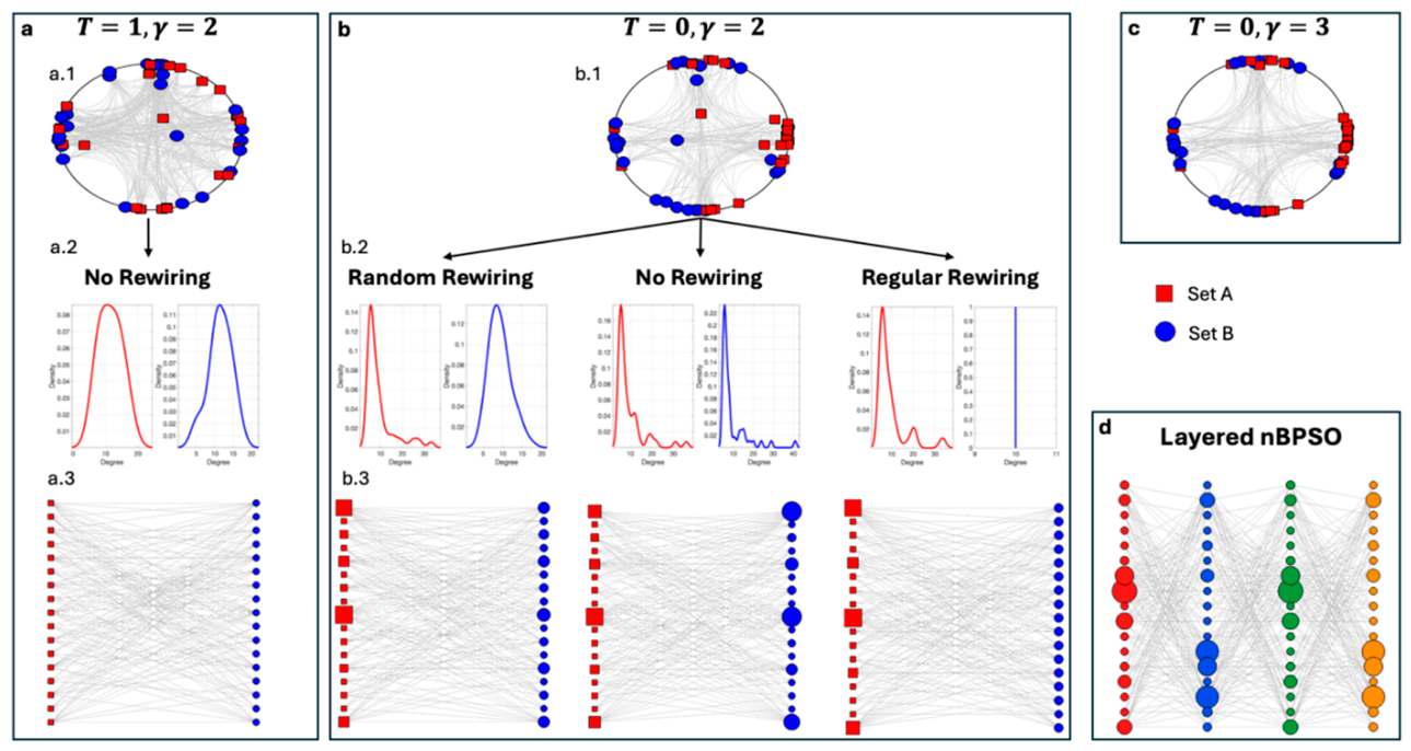
Figure 2.
Community mixing between ground truth communities of nBPSO networks. Fixed parameters are . N is the total number of nodes. T represents the temperature. C is the number of components of the mixture distribution (represents number of communities). Rewiring options are no rewiring, tight, random, or regular. For each parameter combination, 10 networks were generated and the mean value is reported in the heatmap.
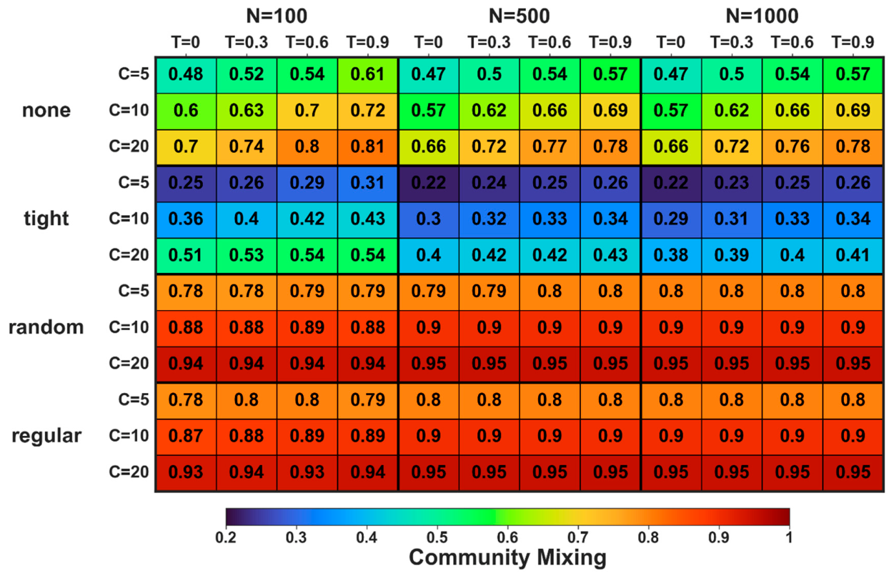
Figure 3.
Robins-Alexander bipartite clustering coefficient [44] of nBPSO networks by temperature (a) and target clustering (b). Fixed parameters are . N is the total number of nodes. T represents the temperature. CC is the target Robins-Alexander bipartite clustering coefficient. C is the number of components of the mixture distribution (represents number of communities). d is the target density. For each parameter combination, 10 networks were generated and the mean value is reported in the heatmap.
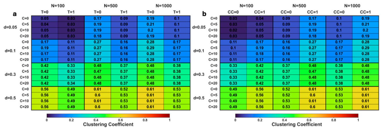
Figure 4.
CIFAR-10 test accuracy for MLPs initialized with layered nBPSO with varying temperatures T with 90% (a), 95% (b), and 99% (c) sparsity and γ = 2, rewiring = none, C = 4. Static models (blue) train weights solely via gradient descent. CHTs models (red) train weights via gradient descent while simultaneously evolving connectivity. Colors go from dark red/blue for initializations with a lower temperature (respecting the underlying geometry) to light red/blue for initializations with a higher temperature (more random). (d) CIFAR-10 test accuracy for MLPs initialized with layered nBPSO with varying levels of γ and sparsity levels, models trained by CHTs and T = 0, rewiring = none, C = 4. (e) CIFAR-10 test accuracy for MLPs initialized with layered nBPSO with different rewiring mechanisms and sparsity levels, trained by CHTs and T = 0, γ = 2, C = 4. ER (Erdős–Rényi like) represents the set which has been randomly rewired. ER − γ = 2 means set A has been rewired, γ = 2 − ER means set B has been rewired, and ER − ER means both sets have been rewired. (f) CIFAR-10 test accuracy for MLPs initialized with layered nBPSO with different number of communities and sparsity levels, trained by CHTs and T = 0, γ = 2, rewiring = none. All have a spreading factor of s = 6. For each parameter combination, 3 seeds were run, the mean value is reported, with the error bars representing the standard error of the mean (SEM).
Disclaimer/Publisher’s Note: The statements, opinions and data contained in all publications are solely those of the individual author(s) and contributor(s) and not of MDPI and/or the editor(s). MDPI and/or the editor(s) disclaim responsibility for any injury to people or property resulting from any ideas, methods, instructions or products referred to in the content. |
© 2026 by the authors. Licensee MDPI, Basel, Switzerland. This article is an open access article distributed under the terms and conditions of the Creative Commons Attribution (CC BY) license.
Copyright: This open access article is published under a Creative Commons CC BY 4.0 license, which permit the free download, distribution, and reuse, provided that the author and preprint are cited in any reuse.